A New Family of Regression Models for $[0,1]$ Outcome Data: Expanding the Palette

Abstract

Beta regression is a popular methodology when the outcome variable $y$ is on the open interval $(0,1)$. When $y$ is in the closed interval $[0,1]$, it is commonly accepted that beta regression is inapplicable. Instead, common solutions are to use augmented beta regression or censoring models or else to subjectively rescale the endpoints to allow beta regression. We provide an attractive new approach with a family of models that treats the entirety of $y\in[0,1]$ in a single model without rescaling or the need for the complications of augmentation or censoring. This family provides the interpretational convenience of a single straightforward model for the expectation of $y\in[0,1]$ over its entirety. We establish the conditions for the existence of a unique MLE and then examine this new family of models from both maximum-likelihood and Bayesian perspectives. We successfully apply the models to employment data in which augmented beta regression was difficult due to data separation. We also apply the models to healthcare panel data that were originally examined by way of rescaling. Keywords: Beta regression; finite mixture distributions; bounded data; Bayesian inference; longitudinal data.

1 Introduction

Beta regression modeling for bounded continuous data $y\in(0,1)$ has attracted increasing interest over the past 20 years. Percentage outcome data such as vulnerability to climate change (Tran et al., 2022), compliance with tax requirements (Dezső et al., 2022), and health-related quality of life (Gheorghe et al., 2017) are recent examples. Pioneering papers on beta regression include Paolino (2001), Kieschnick and McCullough (2003),and Ferrari and Cribari-Neto (2004). The beta distribution is appealing due to its simplicity of expression combined with its flexibility for displaying different shapes with its density. However the flexibility of the beta distribution declines when $y\in[0,1]$. As a result, alternative models are often used with augmented beta regression being a popular choice. In this paper we present a new family of models for $y\in[0,1]$ data. We adopt a mixture modeling approach using beta and power family distributions. This allows us to model the entirety of $y$ simultaneously without excluding the endpoints as in augmented beta regression, yielding different and complementary research insights.

2 Literature Review

In beta regression we assume $y$ follows the beta distribution with PDF

$$p(y|\alpha,\beta)=\begin{cases}\dfrac{\Gamma(\alpha+\beta)}{\Gamma(\alpha)\Gamma(\beta)}y^{\alpha-1}(1-y)^{\beta-1}&\text{if $0\leq y\leq 1$},\\ 0&\text{otherwise,}\end{cases}$$ (1)

where $\alpha>0$ and $\beta>0$. It is common to transform to

$$\mu_{\beta} =\alpha/(\alpha+\beta),$$ (2a)

$$\phi =\alpha+\beta$$ (2b)

where $\mu_{\beta}$ is the expectation and $\phi$ has an interpretation as a precision component. Next the data analyst collects an outcome variable $y$ having $n_{\beta}$ observations and specifies

$$g(\mu_{\beta_{i}})=\eta_{\beta_{i}}=b_{0}+b_{1}x_{1i}+\ldots+b_{J}x_{Ji}$$ (3)

where $x$ refers to the predictor variables, $i$ indexes the observations, $j=1,\ldots,J$ indexes the predictor variables, $\eta_{\beta_{i}}=g^{-1}(\mu_{\beta_{i}})$, and the link function $g(\cdot)$ is chosen by the data analyst. Then (1), (2), and (3) define a model which we call the classic beta regression model to ease future discussion. The parameter $\phi$ may be taken to be a single quantity or optionally may be considered to depend on predictors analogously to (3). Inserting (2) into (1) gives

$$p(y|\mu_{\beta},\phi)=\begin{cases}\dfrac{\Gamma(\phi)}{\Gamma(\mu_{\beta}\,\phi)\Gamma\bigl{(}(1-\mu_{\beta})\phi\bigr{)}}y^{\mu_{\beta}\,\phi-1}(1-y)^{(1-\mu_{\beta})\phi-1}&\text{if $0\leq y\leq 1$},\\ 0&\text{otherwise,}\end{cases}$$ (4)

where $0<\mu_{\beta}<1$ and $\phi>0$. Then (4) and (3) define an equivalent model. We call (1) the standard parameterization and (4) the alternative parameterization below.

Numerous authors have broadened the scope of classic beta regression. For example spatio-temporal beta regression models have been discussed by Kaufeld et al. (2014) and Mandal et al. (2016). Time-series beta regression models have been discussed by Rocha and Cribari-Neto (2008), Guolo and Varin (2014), and Da-Silva and Migon (2016). Random effects and mixed effects versions can be found in Zimprich (2010), Hunger et al. (2012), and Verkuilen and Smithson (2012). Zhao et al. (2014) examined generalizations of the beta regression dispersion structure. Souza and Moura (2016) described multivariate beta regression models while variable dispersion beta regression having parametric link functions have been discussed by Canterle and Bayer (2019).

One key limitation of the classic beta regression model is that the endpoint $y$ values of zero and/or one traditionally have posed challenges. Many authors have used the augmented (also called inflated) beta regression models for such data (Cook et al., 2008; Galivs et al., 2014; Wang and Luo, 2016, 2017; Di Brisco and Migliorati, 2020). Here the analyst partitions the original data of sample size $N$ into multiple subsets. Denote $y_{\beta}$ as the subset where $y\in(0,1)$ with sample size $n_{y_{\beta}}$. Next if $y=0$ observations exist, a variable $z_{0}$ that takes the value 1 when $y=0$ and zero otherwise is created with $n_{z_{0}}$ successes and $N-n_{z_{0}}$ failures. If required, $z_{1}$ is analogously created. The generated data $z_{1}$ and/or $z_{0}$ then augments $y_{\beta}$. One assumes that the likelihood of observing $z_{0}$, $z_{1}$ and $y_{\beta}$ are independent (Ospina and Ferrari, 2010), yielding the likelihood function

$$\ell(y|\cdot)=\prod_{i=1}^{n_{\beta}}p(y_{\beta_{i}}|\cdot)\prod_{i=1}^{N}p(z_{0i}|\cdot)\prod_{i=1}^{N}p(z_{1i}|\cdot),$$ (5)

where a given $z$ may be omitted and $\cdot$ is a placeholder for parameters to be estimated. Binary choice models are used for $z_{0}$ and/or $z_{1}$. The classic beta regression likelihood,

$$\ell(y_{\beta}|\cdot)=\prod_{i=1}^{n_{\beta}}p(y_{\beta_{i}}|\cdot),$$ (6)

appears as the first product term in (5).

Since the product terms in (5) are independent, the numerical results from a maximum likelihood augmented beta regression model can be exactly duplicated by estimating a maximum likelihood classic beta regression with $y_{\beta}$, and then estimating separate binary choice models on $z_{0}$ and $z_{1}$ using maximum likelihood (Ospina and Ferrari, 2010). This may address important research questions. However, observe that modeling the overall expectation of $y\in[0,1]$ by combining regression results from the tripartite vector of variables $(y_{\beta},z_{1},z_{0})$ and correct sample sizes of $n_{\beta},n_{z_{0}}$, and $n_{z_{1}}$ will not be entirely straightforward using the results from (5). From a theoretical angle, it might be challenging to explain that the endpoint of some variables, such as a test score of 100%, arises from an entirely independent statistical process from that of an adjacent value, such as a score of 99.9%. Another area where interpretation may be more involved are models for longitudinal data. If at time $t$ we observe $y_{it}$, $y_{it}$ may fluctuate between product terms in (5) and be treated as continuous or point-valued depending on $t$. This may lead to a loss of precision if a random effect for one observation must be estimated in multiple product terms. A second solution to this problem is to consider models for censored data (Tobin, 1958). Doubly censored models are also possible (Smithson and Verkuilen, 2006; Ospina and Ferrari, 2010) as is a combination of censoring and augmentation (Hwang et al., 2021). Censoring models may be more interpretable for data like exam scores but the computational overhead may be nontrivial when time-series or spatiotemporal modeling is of interest. A third, more recent, solution is to use a mixture distribution that has positive, finite support on $y\in[0,1]$. Regression modeling using a mixture of the beta and rectangular distributions was first proposed by Bayes et al. (2012) and subsequently considered by Ribeiro et al. (2021). Unfortunately a clear methodology for the endpoints was not proposed. Instead, Hahn (2021) proposed a regression model where $y\in[0,1]$ was taken to be a mixture of a beta distribution and a tilting distribution. However, the expectation of the tilting distribution lies in the range $[1/3,2/3]$, partially constraining marginal inference for $y$ in those models. The current paper proposes models that remove this limitation.

3 The Tilting Power Distribution

Tilted beta regression makes use of the tilting distribution which is a mixture of triangular distributions. The triangular distribution is attractive in its simplicity but this comes at a cost of flexibility as described above. van Dorp and Kotz (2002) described the two-sided power distribution as a more flexible alternative to the triangular. Our requirements are first that the distribution is to provide finite density at the endpoints and second to avoid bimodality which would be less attractive for regression in this context. Given the above, we use a distribution with PDF

$$p(y|\nu)=\begin{cases}(|\nu|+1)y^{|\nu|}&\text{if }0\leq y\leq\mathbf{1}(\nu),\\ (|\nu|+1)(1-y)^{|\nu|}&\text{if }\mathbf{1}(\nu)\leq y\leq 1,\\ 0&\text{otherwise}\end{cases}$$ (7)

with $\nu\in\mathbb{R}$. The Heaviside function, $\mathbf{1}(\cdot)$, appears and $\mathbf{1}(0)$ is taken to be 1. The sign of $\nu$ governs the endpoint location (except that $\nu=0$ gives the rectangular distribution). The triangular distribution with mode of 0 arises when $\nu=-1$ while the triangular distribution with mode of 1 arises when $\nu=1$. We can describe (7) as the tilting power distribution. Figure 1 contains a plot of (7) for several values of $\nu$.

Figure 1: Tilting Power Densities for Selected Values of $\nu$

We find that

$$E(Y)=\mu_{T}=\dfrac{\nu\mathbf{1}(\nu)+1}{|\nu|+2},$$ (8)

and $\text{Var}(Y)=\dfrac{|\nu|+1}{(|\nu|+3)(|\nu|+2)^{2}}$. Here $0<\mu_{T}<1$ which is attractive versus the tilting distribution. As (7) is a special case of the two-sided power distribution, further distributional details appear in van Dorp and Kotz (2002). We are now ready to create the desired mixture, namely

$$p(y|\alpha,\beta,\nu,\theta)=\begin{cases}\begin{split}&(1-\theta)f_{1}(\nu)+\theta\dfrac{\Gamma(\alpha+\beta)}{\Gamma(\alpha)\Gamma(\beta)}y^{\alpha-1+I(y=0)}(1-y)^{\beta-1+I(y=1)}\end{split}&\text{if }0\leq y\leq\mathbf{1}(\nu),\\ \begin{split}&(1-\theta)f_{1}(\nu)+\theta\dfrac{\Gamma(\alpha+\beta)}{\Gamma(\alpha)\Gamma(\beta)}y^{\alpha-1+I(y=0)}(1-y)^{\beta-1+I(y=1)}\end{split}&\text{if }\mathbf{1}(\nu)\leq y\leq 1,\\ 0&\text{otherwise.}\end{cases}$$ (9)

where $f_{1}$ is given by (7). Here $0<\theta<1$ is the mixing weight where the beta component ($f_{2}$) dominates as $\theta$ increases. The indicator functions $I(\cdot)$ in $f_{2}$ ensure $f_{2}$ is zero at an endpoint (Hahn, 2021) which is viable here due to the presence of $f_{1}$ with positive density. Clearly

$$E(Y) =(1-\theta)\mu_{T}+\theta\mu_{\beta},$$ (10)

$$=(1-\theta)\dfrac{\nu\mathbf{1}(\nu)+1}{|\nu|+2}+\theta\dfrac{\alpha}{\alpha+\beta},$$ (11)

and the likelihood of $y$ is

$$\ell(y|\alpha,\beta,\nu,\theta)=\prod_{i=1}^{N}p(y_{i}|\alpha,\beta,\nu,\theta)=\prod_{i=1}^{N}(1-\theta)f_{1}(y_{i}|\nu)+\theta f_{2}(y_{i}|\alpha,\beta).$$ (12)

3.1 Predictive Modeling

3.1.1 Model 1 - tilting power beta regression

We may perform predictive modeling by specifying

$$g_{\beta}(\mu_{\beta_{i}}) =\eta_{\beta_{i}}=b_{0}+b_{1}x_{1i}+\ldots+b_{J}x_{Ji},$$ (13a)

$$g_{T}(\mu_{T_{i}}) =\eta_{T_{i}}=c_{0}+c_{1}x_{1i}+\ldots+c_{J}x_{Ji},$$ (13b)

$$g_{\phi}(\phi_{i}) =\eta_{\phi_{i}}=d_{0}+d_{1}x_{1i}+\ldots+d_{J}x_{Ji},$$ (13c)

$$g_{\theta}(\theta_{i}) =\eta_{\theta_{i}}=a_{0}+a_{1}x_{1i}+\ldots+a_{J}x_{Ji}.$$ (13d)

Going forward the subscript for $g$ will be dropped. Here (9), (12) and (13) resemble those of ordinary finite mixture models (e.g., Titterington, 2011, §1.4.4) upon quick review. However $f_{2}$ contributes only $n_{\beta}$ observations to our understanding of $y$ since the indicator functions remove the $N-n_{\beta}$ endpoints from $f_{2}$. Thus we have two latent classes for $y_{\beta}$ but only one (non-)latent class for the endpoints of $y$. For (13b) we find from (8)

$$\nu=\dfrac{2\mu_{T}}{1/2-|\mu_{T}-1/2|}.$$ (14)

3.1.2 Model 2

Suppose we have no special interest in possible latent classes, but are primarily interested in $y$. Equating $\mu_{\beta}$ and $\mu_{T}$ in (10) provides a useful $\mu_{\beta}=\mu_{T}=E(y)$. We then continue with estimation of (12), (13a), (13c), and (13d). For (13b), we replace $\mu_{T}$ with $\mu_{\beta}$ using (14) to obtain the contribution previously provided. This special case of Model 1 is called Model 2. Estimation of (13a) has a useful interpretation as the conditional expectation of $y\in[0,1]$. This can be contrasted with augmented beta regression where the endpoints are excluded and a probability model for being at an endpoint is used instead. Label-switching is of no particular importance to real-world interpretation of Model 2 since there is no presumption of unknown latent classes and the means have been equated. We can call Model 2 a semimixture model since the mixture weights are retained but there is no presumption of differing expectations and since we assign based on known class membership. Lastly we could employ separate mixture weights for each endpoint. For example, $(1-\theta)$ could be rewritten as $(1-\theta)(1-\zeta)$ for $y=0$ and as $(1-\theta)\zeta$ for $y=1$ assuming $0<\zeta<1$. This is an optional choice which could be assessed with model fit measures.

3.1.3 Model 3 - the endpoint heterogeneous beta regression model

In Model 2 we placed the endpoints in $f_{1}$, $y_{\beta}$ in $f_{2}$, and then applied weights $(1-\theta)$ and $\theta$ respectively per (12). We simplify by eliminating $\theta$ and (13d). The power function distribution is equivalent to (1) with $\beta=1$ and it has finite non-zero density at $y=1$. Also the reflected power distribution is equivalent to (1) with $\alpha=1$ and has finite non-zero density at $y=0$. Thus we directly apply the relevant distribution to endpoint observations. Additional details are as follows. We require that $\mu_{\beta}$ remains free to vary in (4), hence $\phi$ must be fixed. Application of (2a) and (2b) yields $\alpha=\mu_{\beta}\,\phi$ and $\beta=(1-\mu_{\beta})\phi$ for insertion into (1). Therefore when $y=1$, applying the constraint $\beta=1$ gives

$$\alpha=\frac{\mu_{T}}{1-\mu_{T}}$$ (15)

and in the alternate parameterization we set

$$\phi=\frac{1}{1-\mu_{T}}$$ (16)

where $\mu_{T}$ has been used for continuity purposes in discussion of the former distribution component $f_{1}$ ($\mu_{\beta}$ could have been used equivalently). When $y=0$, applying the constraint $\alpha=1$ gives

$$\beta=\frac{1-\mu_{T}}{\mu_{T}}$$ (17)

or alternatively

$$\phi=\frac{1}{\mu_{T}}.$$ (18)

As in Model 2, estimation of (13b) is subsumed into estimation of (13a) and is not performed. Next we prove a theorem regarding Model 3.

Theorem 1.

Model 3 constitutes a beta regression model for $y\in[0,1]$ that is estimable by maximum likelihood under certain data conditions.

Proof.

Here we use $\mu$ in place of $\mu_{\beta}$ since there is no mixture involving the mean. Considering the above and (4) we can now write a beta distribution as

$$p(y|\mu,\phi)=\begin{cases}\dfrac{\Gamma(\phi^{*})}{\Gamma(\mu\,\phi^{*})\Gamma\bigl{(}(1-\mu)\phi^{*}\bigr{)}}y^{\mu\,\phi^{*}-1}(1-y)^{(1-\mu)\phi^{*}-1}&\text{if $0\leq y\leq 1$},\\ 0&\text{otherwise,}\end{cases}$$ (19)

where $\phi^{*}>0\ni\phi^{*}=\phi+I(y=0)\biggl{(}\dfrac{1}{\mu}-\phi\biggr{)}+I(y=1)\biggl{(}\dfrac{1}{1-\mu}-\phi\biggr{)}$. When $y\in(0,1)$ the classic beta regression model applies. When $y=0$, $\phi^{*}$ produces the Beta$\bigl{(}1,(1-\mu)/\mu\bigr{)}$ distribution in (1). When $y=1$, $\phi^{*}$ produces the Beta$\bigl{(}\mu/(1-\mu),1\bigr{)}$ distribution in (1). Hence (19) and (13a) constitute a beta regression model for $y\in[0,1]$. ∎

We can call Model 3 the endpoint heterogeneous beta regression model to remind us that $\phi$ is altered at an endpoint. Endpoint observations do not provide information about $\phi$ in Model 3, which is also true of augmented beta regression. Therefore (13c) is omitted for endpoint values. We can also backpropagate this result to Model 2. Namely we replace $f_{1}(y|\nu)$ of (12) with the alternate Beta$\bigl{(}\mu,\phi^{*}\bigr{)}$ distribution. While Model 3 expands the palette of models for $y\in[0,1]$ data, some estimation challenges may arise. We now examine this issue. For reference, (15) in (19) implies the power distribution

$$p(y|\mu)=\begin{cases}\dfrac{\mu}{1-\mu}y^{\frac{\mu}{1-\mu}-1}&\text{if $0<y\leq 1$},\\ 0&\text{otherwise,}\end{cases}$$ (20)

while the reflected power distribution from (17) in (19) is

$$p(y|\mu)=\begin{cases}\dfrac{1-\mu}{\mu}(1-y)^{\frac{1-\mu}{\mu}-1}&\text{if $0\leq y<1$},\\ 0&\text{otherwise,}\end{cases}$$ (21)

Next let $n_{0}\equiv n_{z_{0}}$ be the number of observations where $y=0$ and denote this data as $y_{0}$. Also let $n_{1}\equiv n_{z_{1}}$ be the number of observations where $y=1$ and denote this data as $y_{1}$. Then we may write the three separate portions of the log-likelihood function of Model 3 as

$$\log\ell(y_{0}|\mu) =n_{0}\bigl{(}\log(1-\mu)-\log(\mu)\bigr{)},$$ (22)

$$\log\ell(y_{1}|\mu) =n_{1}\bigl{(}\log(\mu)-\log\left(1-\mu\right)\bigr{)},$$ (23)

$$\begin{split}\log\ell(y_{\beta}|\mu,\phi)&=n_{\beta}\bigl{(}\log\Gamma(\phi)-\log\Gamma(\mu\phi)-\log\Gamma(\phi-\mu\phi)\bigr{)}\\ &\quad+(\mu\phi-1)\sum_{i=1}^{n_{\beta}}\log\left(y_{i}\right)+(\phi-\mu\phi-1)\sum_{i=1}^{n_{\beta}}\log\left(1-y_{i}\right).\end{split}$$ (24)

Previous authors have examined the behavior of (24) (e.g., Ferrari and Cribari-Neto, 2004; Kieschnick and McCullough, 2003). Therefore we focus on (22) and (23). Observe $y$ appears in (22) and (23) only through $n_{0}$ and $n_{1}$ respectively. Briefly consider $y\notin(0,1)$ despite Model 3 not being intended for such. First, if we have $y_{0}$ only (or $y_{1}$ only) clearly the maximum likelihood will be undefined (we would expect poor behavior for degenerate $y$). Second, if we have both $y_{0}$ and $y_{1}$ where $n_{0}=n_{1}$, the likelihood is zero for $0<\mu<1$ since (22) and (23) exactly cancel. Again, estimation of Model 3 is not possible. Third, if we have $y_{0}$ and $y_{1}$ where $n_{0}\neq n_{1}$, clearly the first $\min[n_{0},n_{1}]$ terms will cancel and the likelihood of the remaining $|n_{0}-n_{1}|$ observations will again have an undefined maximum. The cancellation property will be useful below. Furthermore

$$\frac{d}{d\mu}\log\ell(y_{0}|\mu) =\frac{n_{0}}{\mu^{2}-\mu},$$ (25)

$$\frac{d}{d\mu}\log\ell(y_{1}|\mu) =\frac{n_{1}}{\mu-\mu^{2}}$$ (26)

$$\frac{d^{2}}{d\mu^{2}}\log\ell(y_{0}|\mu) =n_{0}\left(\frac{1}{\mu^{2}}-\frac{1}{(1-\mu)^{2}}\right),$$ (27)

$$\frac{d^{2}}{d\mu^{2}}\log\ell(y_{1}|\mu) =n_{1}\left(\frac{1}{(1-\mu)^{2}-\frac{1}{\mu^{2}}}\right).$$ (28)

Challenges include (25) and (26) lacking roots and (27) and (28) possibly having the wrong signs depending on the location of $\mu$ versus the midpoint of the range of $y$. However, (27) is negative when $\mu>1/2$. Combining with (24) we clearly have a global maximum in the parameter space when $y\in[0,1)$ and $\mu>1/2$ given that (24) has its own maximum in the parameter space. Similarly we have a global maximum in the parameter space when $y\in(0,1]$ and $\mu<1/2$ given that (24) has its own maximum in the parameter space. If these conditions do not hold, we may still find we have a local maximum in the vicinity of the maximum for (24). The extent to which there is a local maximum will depend on the magnitudes of $|n_{0}-n_{1}|,n_{\beta},\mu$ and $\phi$. We now examine the data conditions mentioned in Theorem 1 with respect to the existence of a global maximum.

Theorem 2.

Suppose we have $n_{0}$ observations of $y_{0}$ and $n_{\beta}$ observations of $y_{\beta}$. Further assume we have found a global optimum for $\mu$ and $\phi>1$ for $y_{\beta}$. Then the MLEs of $\mu$ and $\phi$ for Model 3 will have a global optimum in the parameter space as long as $n_{\beta}\geq N/2$.

Proof.

Suppose we begin by fitting a classic beta regression model to data consisting of $n_{\beta}$ non-endpoint observations, and that there exists a global optimum in the parameter space $(\mu,\phi)$ for this data. First note that we obviously can re-fit this classic beta regression model with its global optimum by using the log-likelihood of (24) in which the normalizing constants have been omitted. Therefore the global optimum holds for the terms which are a function of $y$, completing the proof for these terms. Next, add $n_{0}$ observations in which $y=0$ to the data and retain only normalizing constants from (24) and (22) to produce

$$n_{\beta}\bigl{(}\log{\Gamma(\phi)}-\log{\Gamma(\mu\phi)}-\log{\Gamma(\phi-\mu\phi)}\bigr{)}+n_{0}\bigl{(}\log(1-\mu)-\log(\mu)\bigr{)}$$ (29)

Upon equating $n_{0}$ and $n_{\beta}$ they can be dropped and we see (29) has a global optimum at approximate values of $\mu=0.247$ and $\phi=3.319$, completing the proof. ∎

Theorem 3.

Suppose we have $n_{0}$ observations of $y_{0}$, $n_{1}$ observations of $y_{1}$, and $n_{\beta}$ observations of $y_{\beta}$. Further assume $\phi>1$ in $y_{\beta}$. Then the MLEs of $\mu$ and $\phi$ for Model 3 will have a global optimum in the parameter space as long as $n_{\beta}\geq N/2$, i.e., as long as the non-endpoint observations constitute at least half of the total observations.

Proof.

The case where $n_{0}>0$ and $n_{1}=0$ was proved above. Suppose $n_{0}=0$ and $n_{1}>0$. The proof of Theorem 2 was based on (21). Here we instead have (20). Clearly then the global optimum exists in the parameter space when $n_{1}=n_{\beta}$ with the associated reflection. Finally when both $n_{0}>0$ and $n_{1}>0$, we have shown above that only $|n_{0}-n_{1}|$ observations will contribute to the likelihood and the remaining endpoint observations will cancel. Therefore, in this case a global maximum exists as long as $n_{\beta}\geq|n_{0}-n_{1}|$, completing the proof. In this case, $n_{\beta}$ may actually be substantially less than $N/2$ and still satisfy $n_{\beta}\geq|n_{0}-n_{1}|$. ∎

Theorem 3 shows that the likelihood of Model 3 may have a global maximum under certain conditions. In practice numerical investigations reveal the bound of Theorem 3 can be loosened slightly. As a simple example, suppose we take $n_{0}=n_{\beta}+\delta$ where $\delta$ is a small constant. Then as $N\rightarrow\infty$, note that $n_{\beta}+\delta\approx n_{\beta}\approx N/2$ so estimation is likely well-behaved for small excursions relative to $N$. In regression models $\mu$ will no longer be a scalar quantity. We can arrive at the following lemma.

Lemma 1.

Suppose we have $n_{0}$ observations of $y_{0}$, and $n_{1}$ observations of $y_{1}$. Then the contribution of these observations to the likelihood when $\mu$ is non-scalar is

$$\sum_{i=1}^{n_{0}}\log\left(1-\mu_{i}\right)-\sum_{i=1}^{n_{1}}\log\left(1-\mu_{i}\right)+\sum_{i=1}^{n_{1}}\log\left(\mu_{i}\right)-\sum_{i=1}^{n_{0}}\log\left(\mu_{i}\right).$$ (30)

Proof.

This follows immediately from (22) and (23). ∎

Now (29) as used for Theorem 2 can be rewritten for non-scalar $\mu$. However determining whether a global optimum exists for a regression parameter $b$ is more difficult since this also depends on $x,b,n_{0},n_{1},n_{\beta}$ and $g(\cdot)$. Hence we may wish to ensure $n_{\beta}\gg|n_{0}-n_{1}|$ for such $b$. As a practical example, a random slopes model may be more difficult to estimate than a random intercepts model. We see that Theorem 3 applies on a per-parameter basis so some parameters may have a global optimum but not others. A local maximum may be available in the vicinity of the classic beta regression’s global maximum as long as $n_{\beta}$ for that parameter is not too much smaller than $N/2$ for that parameter. Thus a prudent estimation procedure for Model 3 would be to first estimate the classic beta regression using only $y_{\beta}$. The parameter estimates from this initial fit would be stored and then used as initial values for estimation of Model 3 on $y$.

3.1.4 Model 4

We have seen the likelihood may become unbounded for a particular parameter when its observations have predominately endpoint values. One approach would be to consider this parameter inestimable and omit it from the model. We now examine an alternative approach to mitigate this issue. Consider the $y=1$ endpoint and recall in (16) we have fixed $\phi$ to satisfy $(1-\mu)\phi=1$. Consider now fixing $\mu$ instead. In doing so we would set

$$\mu=\frac{\phi-1}{\phi}$$ (31)

which holds under the previous requirement that $\phi>1$. Now that $\phi$ is free to vary, (16) shows that $\mu$ will now approach 1 as $\phi\rightarrow\infty$ (the expectation of the transformed version of (20) behaves similarly). Next let us reexamine the power distribution of (20). Making the substitution of (31) yields a likelihood of $\phi-1$ when $y=1$. We could therefore consider an upper bound for the likelihood of the power distribution to be $\phi-1$ by the above logic considering the role of $\phi$. The appropriate logic applied to the reflected power distribution of (21) also gives an upper bound of $\phi-1$ for the likelihood when $y=0$.

We next note an influential concept discussed by Verkuilen and Smithson (2012, p. 87). Verkuilen and Smithson (2012) advised one may nudge endpoint values away from the endpoint using a personally-chosen delta such as 0.001. This rescales observations to values between, say, 0.001 to 0.999, permitting classic beta regression modeling. Applying this concept, suppose we consider the limit of (4) as both $y$ and $\mu_{\beta}$ approach the endpoint of 1 at the same rate. That is, define $\tilde{\mu}\equiv\mu_{\beta}=y$ and note that if we could vary both $y$ and $\mu_{\beta}$ infinitesimally away from the endpoint at the same rate, we would have

$$\lim_{\tilde{\mu}\to 1}p(y|\mu_{\beta},\phi)=\lim_{\tilde{\mu}\to 1}p(\tilde{\mu}|\tilde{\mu},\phi)=\phi.$$ (32)

This would be the upper bound of the likelihood under these conditions and is close to the upper bound $\phi-1$ previously obtained. While (Verkuilen and Smithson, 2012) advise sensitivity analyses for the personal choice of delta, here we do not select a particular numeric delta but instead consider a true infinitesimal in terms of a limit.

Now suppose we have a parameter for which Theorem 3 does not hold, $\check{\mu}$. Writing $\check{\mu}=g^{-1}(\check{\eta})$, for Model 4 we require that the likelihood satisfies

$$\dfrac{g^{-1}(\check{\eta})}{1-g^{-1}(\check{\eta})}\leq U$$ (33)

using the power distribution and similarly we require that

$$\dfrac{1-g^{-1}(\check{\eta})}{g^{-1}(\check{\eta})}\leq U$$ (34)

using the reflected power distribution, where $U$ is an upper bound such as $(\phi-1)$ or $\phi$. We now have the endpoints’ contribution to the likelihood for Model 4. This is

$$\begin{split}\log\ell(y_{i}|\cdot)&=I(y_{i}=0)I(q_{i}=0)\bigl{(}\log(1-\mu_{i})-\log(\mu_{i})\bigr{)}\\ &\quad+I(y_{i}=1)I(q_{i}=0)\bigl{(}\log(\mu_{i})-\log(1-\mu_{i})\bigr{)}+I(0<y_{i}<1)\log\ell(y_{\beta_{i}}|\cdot)\\ &\quad+I(y_{i}=0)I(q_{i}=1)\min\bigl{(}\log(1-\dfrac{g^{-1}(\eta_{i})}{1-g^{-1}(\eta_{i})})-\log(\dfrac{g^{-1}(\eta_{i})}{1-g^{-1}(\eta_{i})}),U_{i}\bigr{)}\\ &\quad+I(y_{i}=1)I(q_{i}=1)\min\bigl{(}\log(\dfrac{g^{-1}(\eta_{i})}{1-g^{-1}(\eta_{i})})-\log(1-\dfrac{g^{-1}(\eta_{i})}{1-g^{-1}(\eta_{i})}),U_{i}\bigr{)},\end{split}$$ (35)

where $q_{i}$ takes the value one if Theorem 3 does not hold for the parameter and zero otherwise, $U_{i}$ is a likelihood upper bound for a group mean such as $(\phi-1)$ or $\phi$, and $\log\ell(y_{\beta_{i}})$ is the classic beta regression log-likelihood of (24). It can be shown that (35) simplifies when $g$ is the logit link. In this case we can then omit $q_{i}$ and instead place a constraint directly on the parameter in $\check{\eta}$ for which Theorem 3 does not hold. Namely we can require that $|\check{\eta}_{i}|\leq\log U_{i}$ when we are estimating $\check{\mu}$. Then the two final terms in (35) reduce to $I(y_{i}=0)\bigl{(}\log(1-\check{\mu}_{i})-\log(\check{\mu}_{i})\bigr{)}+I(y_{i}=1)\bigl{(}\log(\check{\mu}_{i})-\log(1-\check{\mu}_{i})\bigr{)}$. But then application of the constraint $|\eta_{i}|\leq\log U_{i}\forall\check{\mu}_{i}$ implies we no longer need the last two terms of (35) because $\check{\mu}$ no longer needs a separate treatment in the log-likelihood function. Instead we can use the log-likelihood from Model 3. This is convenient because we can quickly identify situations where Theorem 3 may not hold using descriptive statistics. We can then constrain the relevant parameters and use the log-likelihood function from Model 3, namely the sum of (22), (23) and (24). It is rare to see classic beta regression with non-logit link functions, so this simplification can be used often. However, if $\check{\eta}$ does not arise from a group mean parameter, that is to say if $\check{\eta}$ results from a continuous predictor such as $\check{\eta}_{i}=\check{b}x_{i}$ where $x_{i}$ is not constant across observations, then the simplification based on constraining $\check{b}$ also does not hold. In this situation (35) would again need to be used.

Model 4 has some attractive features for analysts who would otherwise be rescaling. First, there is no need to personally devise multiple delta values and perform sensitivity analyses on them. In big-data contexts we may find that different delta choices have different kinds of impacts, complicating matters. Next it is attractive we can constrain some (possibly few) parameters instead of rescaling a larger number of data points. Further the likelihood function can by itself move toward a larger value of $\phi$ if it improves overall model fit without the need of personal analyst choices. Finally if the corresponding classic beta regression model has appreciable information about $\phi$, $\phi$ can provide anchoring to the likelihood for $\check{\mu}$. The disadvantage can be seen with reference to (10). Recall that a novel aspect of Models 2 and 3 is that they model the expectation of $Y$ over its entire range. In Model 4 we can only make an approximate statement about the expected value of the endpoint observations (i.e, about $\mu_{T}$ in (10)). As a result the equality in (10) must be replaced such that

$$E(Y)\approx(1-\theta)\mu_{T}+\theta\mu_{\beta},$$

if the Model 4 upper bound is applied to Model 2 (the inequality also carries over to Model 3). However, it should be noted that both augmented beta regression and classic beta regression using rescaling will also not satisfy the equality given by (10) when $y\in[0,1]$. Predicted values from Model 4 may be created as in for Model 3 with the extra step of accounting for $U$ as needed.

4 Applications

The Financial Times (Financial Times, 2022) provides annual data on top-100 ranked Master’s of Business Adminstration (MBA) programs worldwide. Our $y$ is the percentage of MBA graduates from a program who are employed at three months after graduation. One to five observations of $y=100\%$ occurred per year (but no zeros) in the period 2012 to 2021. The list composition changed from year to year as rankings changed, and occasional ties meant more than 100 programs could appear. Stata software version 16 with package zoib (Buis, 2010) was used for the augmented beta regression. We had planned to use five independent variables for analysis of an arbitrary year. Interestingly we found that the logit portion of the augmented beta regression model did not appear well-behaved except for in 2012. Stata’s zoib command produced $d$ estimates with implausibly large values (to be discussed in Table 2) while Stata’s logit command provided a warning message (and sometimes would not produce estimates). We then noted Albert and Anderson (1984) showed that the logit model may have no MLE if the data exhibits complete or quasicomplete separation. This was the problem here. We report on a smaller more well-behaved model with 2016 data for ease of comparison and defer the problem of data separation until later. Our predictor variables were the percentage of international students enrolled in the program ($x_{1}$), the percentage of international members on university’s board ($x_{2}$), and the percentage of full-time faculty with doctorates ($x_{3}$). Results appear in Table 1. For ease of comparison we place the one-augmented beta regression logit model $d$ coefficients in rows that correspond to the $d$ coefficients from (13d).

Table 1: Percent employed after graduation, 2016: Maximum likelihood parameter estimates, standard errors and $z$ statistics.

	Augmented	Model 1	Model 2	Model 3	Model 2	Model 2
	B.R.				with (13d)	with (13d)
Para-						and $\mathbf{X}_{\beta}$
meter	($y_{\beta}$ & $z_{1}$)	($y$)	($y$)	($y$)	($y$)	($y$)
$b_{0}$	2.2994	2.3609	2.3156	2.3156	2.3156	2.2994
	(0.6444)	(0.6046)	(0.6496)	(0.6496)	(0.6496)	(0.6449)
	3.568	3.905	3.565	3.565	3.565	3.566
$b_{1}$	-0.0061	-0.0097	-0.0069	-0.0069	-0.0069	-0.0061
	(0.0025)	(0.0027)	(0.0026)	(0.0026)	(0.0026)	(0.0025)
	-2.415	-3.597	-2.701	-2.701	-2.701	-2.414
$b_{2}$	-0.0004	0.0021	-0.0001	-0.0001	-0.0001	-0.0004
	(0.0028)	(0.0027)	(0.0028)	(0.0028)	(0.0028)	(0.0028)
	-0.152	0.775	-0.037	-0.037	-0.037	-0.152
$b_{3}$	0.0009	0.0026	0.0013	0.0013	0.0013	0.0009
	(0.0073)	(0.0069)	(0.0073)	(0.0073)	(0.0073)	(0.0073)
	0.131	0.370	0.184	0.184	0.184	0.131
$d_{0}$	-2.2286				2.2286	2.2286
	(4.6172)				(4.6172)	(4.6172)
	-0.483				0.483	0.483
$d_{1}$	-0.0507				0.0507	0.0507
	(0.0262)				(0.0262)	(0.0262)
	-1.937				1.937	1.937
$d_{2}$	0.0154				-0.0154	-0.0154
	(0.0224)				(0.0224)	(0.0224)
	0.685				-0.685	-0.685
$d_{3}$	0.0071				-0.0071	-0.0071
	(0.0503)				(0.0503)	(0.0503)
	0.142				-0.142	-0.142
$\log(\phi)$	3.1185	3.9916	3.1325	3.1325	3.1325	3.1185
	(0.1446)	(0.3476)	(0.1428)	(0.1428)	(0.1428)	(0.1446)
	21.568	11.484	21.937	21.937	21.937	21.567
logit$(\theta)$		0.3657	3.1884
		(0.4697)	(0.5102)
		0.779	6.249
AIC	-224.88	-270.72	-243.64	-279.31	-242.62	-224.88

Model outcome variable(s), $y_{\beta}$ & $z_{1}$ or $y$, listed below model name.

We see that $b_{1}$ is significant at the $p<0.05$ level in augmented beta regression while $d_{1}$ is marginally significant. The $b_{1}$ coefficient in Model 1 is also significant and the coefficient is further from zero. Model 1 has a larger value of $\log(\phi)$ (3.9916 vs. 3.1185) but is less precisely estimated. Inverting the logit transformation for Model 1’s $\theta$ gives a value of 59.04%. This suggests that the tilting power component applies to a sizable portion of the observations. Model 2 provides similar findings for $b_{1}$ but $\theta$ is 96.04% (logit$(\theta)=3.1884$) since the data set has four observations of 1 out of $N=101$. Model 3 omits $\theta$ entirely. We see the Model 3 coefficients are identical to those of Model 2 excepting the omitted $\theta$ parameter. The final columns of Table 1 report Model 2 estimates when (13d) is additionally estimated. We see that the value of $d_{0}$ through $d_{3}$ replicate those obtained by the one-augmented beta regression model with the exception of a sign change.

4.1 Classical Model Comparison

Table 1 includes AIC for all models.More formal comparisons of augmented beta regression and our Model 2 are also possible. Define the matrix $\mathbf{X}^{+}$ of dimension $N\times(j+1)$ which consists of the $j$ predictor variables and also a constant unity intercept column. Next define the $N\times N$ matrix $\mathbf{U}$ with nondiagonal elements of 0, diagonal element 0 on row $i$ if $y_{i}$ is an endpoint, and diagonal element 1 otherwise. Form $\mathbf{X}_{\beta}=\mathbf{UX}^{+}$ of dimension $N\times(j+1)$ where rows corresponding to endpoint values of $y_{i}$ have entries of zero. Lastly suppose we only observe one endpoint but not both in our data, as we do here. Then Model 2 using $\mathbf{X}_{\beta}$ allows us to replicate the coefficient vector $\mathbf{b}_{\beta}$ which is the vector of $b$ coefficients produced by augmented beta regression and classic beta regression when endpoints have been excluded. Additionally estimating (13d) in this version of Model 2 will further replicate the augmented beta $d$ coefficients up to a sign change (last column of Table 1). The AIC value of -224.88 obtained for this model also replicates the AIC of the augmented beta regression in the Table 1. Next we examine Wald tests. Using Table 1’s Model 2 with (13d) and $\mathbf{X}_{\beta}$, a Wald test of coefficients excluding intercepts ($b_{1}=-d_{1},\ldots,b_{3}=-d_{3}$) gives $\chi^{2}(3)=3.10,p=0.376$. The Wald test including intercepts ($b_{0}=-d_{0},\ldots,b_{3}=-d_{3}$) gives $\chi^{2}(4)=83.65,p<0.0001$. For augmented beta regression, a Wald test of ($b_{1}=d_{1},\ldots,b_{3}=d_{3}$) also gives $\chi^{2}(3)=3.10,p=0.376$ and the Wald test with intercepts ($b_{0}=d_{0},\ldots,b_{3}=d_{3}$) again gives $\chi^{2}(4)=83.65$ with $p<0.0001$. As a final test, we can compute the likelihood ratio of Model 2 without $d$ coefficients (middle columns of Table 1) versus Model 2 with (13d) $d$ coefficients (final columns of Table 1). This gives $\chi^{2}(3)=4.98,p=0.1734$. We conclude an absence of significant differences between Model 2’s predictive model for $\hat{y}$ and Model 2’s endpoint probability model.

4.2 Model Diagnostics

One benefit of the proposed Models is many standard model diagnostic techniques will work for the entirety of $y$ with minimal modification since $y$ does not need a tripartite conceptualization. For example, Figure 2 plots predicted versus observed values for $y\in[0,1]$. This allows simultaneous examination of model fit properties for endpoint and non-endpoint values. A residual plot would also be straightforward since we need not concern ourselves with $z_{0}$ and/or $z_{1}$. We can also create a scatter plot of $g(\hat{\mu}_{y})$ and $g(\hat{\theta})$ when using Model 2 with (13d) (Figure 2). These plots would be less straightforward to create in augmented beta regression. Model 3 in particular should inherit many classic beta regression model diagnostics with minor modifications since we have shown it to be a member of the classic beta regression model family. For example, Ferrari and Cribari-Neto (2004, p. 806) proposed the standardized residual for classic beta regression as

$$r_{i}=\frac{y_{i}-\mu_{i}}{\sqrt{\textrm{Var}(y_{i})}}$$

where $\textrm{Var}(y_{i})=\mu_{i}(1-\mu_{i})/(\phi+1)$. We may use this expression for Model 3 subject to the revision that $\textrm{Var}(y_{i})=\mu_{i}(1-\mu_{i})/(\phi^{*}+1)$ where $\phi^{*}$ is as in the proof of Theorem 1.

Figure 2: Example diagnostic plots: 2016 Percent employed after graduation data

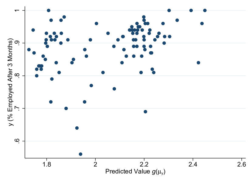
(a) Model 3 observed $y$ vs. predicted $g(\mu)$.

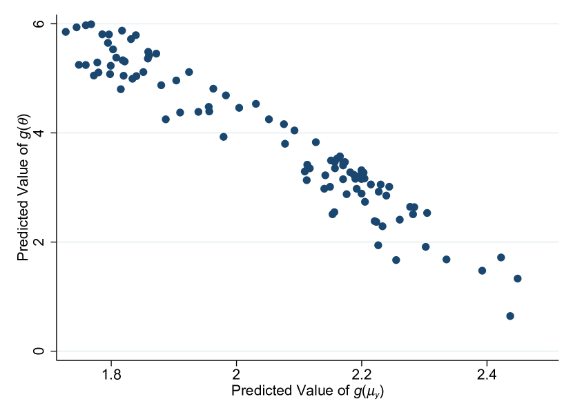
(b) Model 2 with (13d)

One application of the models in this paper is to fit data for which augmented beta regression is unsuccessful due to partial or complete data separation (Albert and Anderson, 1984; Allison, 2004) in the logit portion of the model. The yearly subsets of our data exhibited partial or complete data separation in all years except one. Table 2 provides example results for 2014 data. The $b$ coefficients for the augmented beta regression model appear reasonable but the $d$ ones appear less so. The $b$ coefficients for Model 3 appear reasonable and also allow us to draw conclusions about $y\in[0,1]$. Model 2 with (13d) omitted produces $b$ estimates that are identical to those of Model 3 as expected (results omitted for economy). Also as expected, Model 2 with (13d) produces problematic $d$ estimates just like augmented beta regression (results omitted). We see this phenomenon is not intrinsic to augmented beta regression but is instead intrinsic to the binary logit model (which our semimixture Model 2 with (13d) replicates). Models 1 through 4 can omit (13d), avoiding this problem. Allison (2004) gives recommendations for addressing data separation.

Table 2: Percent employed after graduation, 2014: Estimates comparison

	Augmented		Model 3
	B.R.
Para-	MLE		MLE
meter	(S.E.)	$z$	(S.E.)	$z$
$b_{0}$	1.934	2.29	1.982	2.35
	(0.8433)		(0.8453)
$b_{1}$	-0.0061	-2.26	-0.0065	-2.40
	(0.0027)		(0.0027)
$b_{2}$	0.0003	0.12	0.0006	0.20
	(0.0027)		(0.0027)
$b_{3}$	0.0020	0.22	0.0017	0.18
	(0.0089)		(0.0090)
$d_{0}$	1105.9	0.02
	(48627.2)
$d_{1}$	-8.648	-0.02
	(385.5)
$d_{2}$	2.422	0.02
	(116.3)
$d_{3}$	-12.46	-0.02
	(548.3)
$\log(\phi)$	2.805	19.72	2.809	19.82
AIC	-213.82		-226.00

4.3 Panel Data

Panel data is a context where the relevance of Model 4 may increase. For example, short panels or high serial correlation may lead to a situation where an individual-level fixed or random effect may have numerous endpoint observations. Per Theorem 3 a global optimum may not for exist such parameters. We explore several formulations of panel data models here and adopt a Bayesian viewpoint. The Financial Times data set consists of 990 observations from 131 universities over the years 2012–2021 (universities that only appeared in the rankings once were dropped to ensure that repeated observations were available for each unit of analysis). 31 of the 990 observations were at the endpoint of 1. We estimate a random-intercepts model as follows

$$\textrm{logit}(\mu_{\beta_{it}}) =\eta_{\beta_{it}}=b_{0}+b_{1}x_{1it}+\ldots+b_{3}x_{3it}+m_{i},$$

$$b_{0},b_{1},b_{2},b_{3} \sim\textrm{Normal}(0,0.04),$$

$$\phi \sim\textrm{Uniform}(3,150),$$ (36)

$$m_{i} \sim\textrm{Normal}(0,\sigma_{m}),$$

$$\sigma_{m} \sim\textrm{Exponential}(\cdot)$$

where the $m_{i}$ are individual-specific random intercepts drawn from a distribution and $\sigma_{m}$ is the standard deviation of the random intercepts. The prior for $\phi$ is bounded away from the U-shaped beta distributions per the above discussion. We consider both $\sigma_{m}\sim\textrm{Exponential}(0.5)$ and $\sigma_{m}\sim\textrm{Exponential}(0.2)$ to examine prior sensitivity. We also perform sensitivity analysis regarding the use of hierarchical centering (Gelfand et al., 1995). In hierarchical centering (HC) $b_{0}$ is removed from the first-level functional form and then relocated to be the mean for the random effects, yielding $m_{i}\sim\textrm{Normal}(b_{0},\sigma_{m})$. This modeling choice typically improves the behavior of the Markov chain and it appears in Table 3 as HC 1. Next consider the equality $\mu=c+(\mu-c)$. We can insert a constant $c$ into a functional form, which will cause the resulting parameter $\mu-c$ to move toward or away from $U$. Thus we also estimate HC 2 where $b_{0}$ is relocated as in HC 1 and a fixed user-specified constant $c$ is inserted as a first-level intercept. Here we chose $c=3$ for HC 2. For bounds, the 31 endpoint observations tend to be clustered within certain universities. There were 6 universities for which the endpoint value of 1 was present in 50% or more of its observations. We placed a bound $U=\phi-1$ on the random intercept for these 6 universities. The remaining random intercepts were left unbounded since they satisfied the conditions for Theorem 3 to hold. We discarded the first 5,000 warm-up iterations of the Markov chains and used 200,000 subsequent iterations for estimation. Convergence checks revealed no concerning issues. Table 3 displays posterior means and 95% credible intervals for our models. Predictor variables are as in Table 1. We include DIC and $p_{d}$ (Spiegelhalter et al., 2002) and WAIC and $p_{W}$ (Watanabe, 2010) as model fit measures.

Table 3: Percent employed after graduation, 2012-2021: Posterior means, 95% credible intervals (in parentheses), and model fit measures

	Model 4	Model 4	Model 4	Model 4
Para-	Prior 1	Prior 2	HC 1	HC 2
meter	$\sigma_{m}\sim\textrm{Exp(0.2)}$	$\sigma_{m}\sim\textrm{Exp(0.5)}$	$\sigma_{m}\sim\textrm{Exp(0.2)}$	$\sigma_{m}\sim\textrm{Exp(0.2)}$
$b_{0}$	2.014	2.019	2.000	-0.9801
	(1.893, 2.144)	(1.89, 2.15)	(1.881, 2.12)	(-1.111, -0.8448)
$b_{1}$	-0.0012	-0.001262	-0.001722	-0.0012
	(-0.0048, 0.0025)	(-0.0048, 0.0024)	(-0.0051, 0.0017)	(-0.0047, 0.0024)
$b_{2}$	0.0007	0.0007	0.0007	0.0007
	(-0.0018, 0.0033)	(-0.0019, 0.0033)	(-0.0018, 0.0033)	(-0.0019, 0.0033)
$b_{3}$	0.0056	0.0055	0.0055	0.0055
	(-0.0022, 0.0135)	(-0.0025, 0.0134)	(-0.0025, 0.0133)	(-0.0024, 0.0135)
$\delta_{m_{1}}$	5.37E-06	0	0.0070	0
	(0, 0)	(0, 0)	(0, 0.0617)	(0, 0)
$\delta_{m_{2}}$	0.0004	0.0004	0.0440	2.57E-05
	(0, 0)	(0, 0)	(0, 0.4451)	(0, 0)
$\delta_{m_{3}}$	1.80E-06	4.11E-06	0.01822	0
	(0, 0)	(0, 0)	(0, 0.2642)	(0, 0)
$\delta_{m_{4}}$	5.88E-07	6.65E-07	0.0064	0
	(0, 0)	(0, 0)	(0, 0.0349)	(0, 0)
$\delta_{m_{5}}$	0.0095	0.0095	0.0883	0.0025
	(0, 0.1422)	(0, 0.1424)	(0, 0.5682)	(0, 0)
$\delta_{m_{6}}$	0	0	0.009478	0
	(0, 0)	(0, 0)	(0, 0.1271)	(0, 0)
$\pi_{U_{1}}$	0.00004	0	0.0323	0
	(0, 0)	(0, 0)	(0, 1)	(0, 0)
$\pi_{U_{2}}$	0.0022	0.0023	0.2078	0.0002
	(0, 0)	(0, 0)	(0, 1)	(0, 0)
$\pi_{U_{3}}$	0.00002	0.000015	0.0858	0
	(0, 0)	(0, 0)	(0, 1)	(0, 0)
$\pi_{U_{4}}$	0.00002	0.000015	0.02901	0
	(0, 0)	(0, 0)	(0, 1)	(0, 0)
$\pi_{U_{5}}$	0.0661	0.0642	0.4248	0.0177
	(0, 1)	(0, 1)	(0, 1)	(0, 0)
$\pi_{U_{6}}$	0	0	0.0436	0
	(0, 0)	(0, 0)	(0, 1)	(0, 0)
$\phi$	45.25	45.25	45.42	45.23
	(41.04, 49.67)	(41.05, 49.69)	(41.19, 49.85)	(40.99, 49.66)
$\sigma_{m}$	0.7188	0.7187	0.6638	0.7335
	(0.6098, 0.8458)	(0.6090, 0.8460)	(0.5744, 0.7674)	(0.615, 0.8769)
DIC	-3320.53	-3320.53	-3299.11	-3324.48
$p_{D}$	123.65	123.62	123.77	123.88
WAIC	-3300.53	-3300.48	-3284.39	-3302.12
$p_{W}$	127.51	127.58	122.53	130.20
MSE	0.002724	0.002725	0.002739	0.002723

We strongly suggest multiple chains that begin with different starting points when estimating our Models. Here we have purposely sought out and used a single chain with initial values that would cause Model 3 to quickly terminate with numerical problems. We have intentionally used this problematic chain by itself to magnify the diagnostic measures reported in Table 3. One diagnostic measure is $\delta_{m}$, which is the difference in the random intercept before and after being bounded by (33). The second is $\pi_{U}$. This took the value one if the corresponding bound was exceeded and zero otherwise, estimating a parameter’s probability of exceeding its bound. The Table documents variability among $\pi_{U}$. For example, University 6’s random intercept was relatively well-behaved except in the HC 1 model ($\pi_{U_{6}}=0.0456$). Conversely University 5’s random intercept was poorly-behaved except in the HC 2 model ($\pi_{U_{5}}=0.0177$).

Comparing models, we see that Model 4 Prior 1 and Model 4 Prior 2 give similar results. HC 1 gave improved estimation of $b_{0}$ according to effective sample size (ESS, Plummer et al., 2006). ESS for $b_{0}$ was 86,008 in this formulation which can be compared to ESS of around $1,050$ for the non-HC formulations. However, HC 1 leads to the least attractive values of $\pi_{U}$. In HC 1 the relocation of $b_{0}$ has pushed the values of $m_{i},\ldots,m_{6}$ much closer to the bound. Insertion of $c=3$ as a first-level intercept in HC 2 improves these diagnostics substantially. Since $c$ does not require estimation, chain performance for $b_{0}$ remains attractive in HC 2 ($b_{0}$ ESS = 87,241). We can recover the posterior mean of $b_{0}$ for HC 2 as $3+-0.9801=2.0199$. Interpretation of $\pi_{U}$ is in its preliminary stages but it may be concerning if the 95% credible interval for $\pi_{U}$ contains the value of 1 (i.e., $\pi_{U}>0.05$). We see that the non-HC models give largely similar estimates to HC 2 and all $\pi_{U}$ measures are small except for $\pi_{U_{5}}$ which is near 0.05.

Examination of model fit measures such as DIC and WAIC may be incorporated. Here we see the best fitting model by DIC and WAIC is HC 2 by a small margin. However, this may be due to $\mu-c$ being closer to the prior mean. For additional sensitivity analysis, we explored a small reduction in $c$ from 3 to 2 (DIC = -3320.90, WAIC = -3300.59) and a small increase from 3 to 4 (DIC = -3327.58, WAIC = -3303.67). Both WAIC and DIC changed (in part due to prior/posterior differences) but WAIC seemed more stable once an adequate user constant had been selected. Both DIC and WAIC are affected by the universities that do not satisfy Theorem 3. University 5 has seven consecutive boundary values of 1 and an eighth of 0.98. Alternative modelling strategies might be to exclude this university’s $y$ and separately model its $z_{1}$ along with other $z_{1}$s (as in augmented beta regression).

4.4 Analysis of Rescaled Healthcare Data

Gheorghe et al. (2017) examined the decline in health-related quality of life (HRQOL) that occurs as people age. They hypothesized that it is not aging but instead time to death (TTD) that is a more important predictor of health declines in the aged. They used Bayesian mixed beta regression to examine this in a sample drawn from the Netherlands. Their data was $y\in(0,1]$ where $y=1$ indicates full health as measured by responses to the SF-6D health questionnaire. Gheorghe et al. (2017) described rescaling endpoint values of 1 to 0.99 in the vein of Smithson and Verkuilen (2006). Here we apply Model 2 to Gheorge et al.’s panel data using portions of their code (available from their publication).

Table 4: Health-related quality of life: Posterior means and 95% credible intervals (in parentheses)

		Beta Regression	Model 2
Variable	Parameter	Rescaled $y\in(0,0.99]$	$y\in[0,1]$
	$b_{0}$	1.282	1.236
		(1.210, 1.355)	(1.172, 1.302)
Age	$b_{1}$	-0.0036	-0.0027
		(-0.0140, 0.0067)	(-0.0114, 0.0062)
Gender	$b_{2}$	-0.2179	-0.2014
		(-0.3627, -0.0705)	(-0.3293, -0.0731)
TTD	$b_{3}$	0.0017	0.0016
		(0.0005, 0.0028)	(0.0006, 0.0027)
	$d_{0}$		4.240
			(3.507, 5.066)
Age	$d_{1}$		-0.0151
			(-0.1120, 0.0799)
Gender	$d_{2}$		-0.2017
			(-0.3372, -0.0675)
TTD	$d_{3}$		0.0001
			(-0.0132, 0.0135)
	$\phi$	25.89	25.91
		(21.08, 31.20)	(20.34, 31.98)

We restrict ourselves to 556 responses data on 356 individuals where missingness did not occur. Ten observations where HRQOL was 0.99 were rescaled back to 1. We used the functional form of their Table 4 Model 6 which has individual-specific random effects and their priors with one exception. We used $\phi\sim\textrm{Uniform}(3,200)$ while their prior was on the reciprocal of $\phi$. Estimation was based on two chains started from different initial values. Each chain had 5000 iterations of burn-in, and a subsequent 200,000 iterations were retained. The two chains converged to a common distribution for all parameters. All ESS’s for the $b$ parameters were greater than 4500. All ESS’s for the $d$ parameters were greater than 1400. Results appear in Table 4. We include descriptors (age, gender, and TTD) to promote comparison with Gheorghe et al. (2017). Table 4 shows that the $b$ coefficients from classic beta regression using rescaled data are similar to those of Model 2. Model 2’s $b$ coefficients are slightly smaller and also have narrower 95% credible intervals. Both models indicate males have lower HRQOL than females ($b_{2}$), and that greater TTD predicts better HRQOL ($b_{3}$). Model 2 also produces $d$ coefficients for insights about endpoint observations, extending their findings. Per $d_{2}$, females are more likely to report perfect health ($y=1$) than are males.

5 Concluding Remarks

It is commonly believed that the beta distribution cannot be used for $y\in[0,1]$ data (Zhou and Huang, 2022; Ospina and Ferrari, 2010, p. 124). This paper expands the palette of models for $y\in[0,1]$ by providing an endpoint-heterogeneous beta regression model for $y\in[0,1]$ (Model 3), three additional closely-related beta regression models, and allowing the first unconstrained modeling of the marginal expectation without data rescaling. Despite our contrasting modeling approach and likelihood functions, in certain cases we can exactly replicate results obtained by augmented beta regression (up to a possible coefficient sign change which does not affect coefficient $p$ values or model comparison measures). Hence in addition to our contributions of new models for $y\in[0,1]$ data, we provide a new lens for viewing augmented beta regression and its binary logit formulation. The models can have varying amounts of parsimony in that we can assign both endpoints to the tilting power component in Model 2 (instead of treating them separately) or by treating all observations in a unified manner (Model 3) using endpoint-heterogeneity. This parsimony may be useful for interpretation and advantageous in complex situations such as NMAR data or spatiotemporal applications. The models are robust to data separation when (13d) is omitted. As for limitations, a unique MLE may not always exist, particularly when only one endpoint predominates in that parameter’s $y$. The existence can be readily checked for group means and intercepts as shown above; for slope parameters a simple check remains an area of research and options include omitting the parameter or using Model 4.

References

- Albert and Anderson (1984) Albert A, Anderson JA. On the existence of maximum likelihood estimates in logistic regression models. Biometrika 1984;71(1); 1–10.
- Allison (2004) Allison P. Convergence problems in logistic regression. In: Altman M, Gill J, McDonald MP (Eds.), Numerical Issues in Statistical Computing for the Social Scientist, Wiley, Hoboken, NJ. pp. 238–252.
- Bayes et al. (2012) Bayes CL, Bázan JL, García C. A new robust regression model for proportions. Bayesian Analysis 2012;7(4); 841–866.
- Buis (2010) Buis ML. ZOIB: Stata module to fit a zero-one inflated beta distribution by maximum likelihood. Statistical Software Components S457156, Boston College Department of Economics, revised 08 Aug 2012, 2010.
- Canterle and Bayer (2019) Canterle DR, Bayer FM. Variable dispersion beta regressions with parametric link functions. Statistical Papers 2019;60; 1541–1567.
- Cook et al. (2008) Cook DO, Kieschnick R, McCullough B. Regression analysis of proportions in finance with self selection. Journal of Empirical Finance 2008;15(5); 860–867.
- Da-Silva and Migon (2016) Da-Silva CQ, Migon HS. Hierarchical dynamic beta model. Revstat-Statistical Journal 2016;14(1); 49–73.
- Dezső et al. (2022) Dezső L, Alm J, Kirchler E. Inequitable wages and tax evasion. Journal of Behavioral and Experimental Economics 2022;96; 101811.
- Di Brisco and Migliorati (2020) Di Brisco AM, Migliorati S. A new mixed-effects mixture model for constrained longitudinal data. Statistics in Medicine 2020;39(2); 129–145.
- Ferrari and Cribari-Neto (2004) Ferrari SLP, Cribari-Neto F. Beta regression for modelling rates and proportions. Journal of Applied Statistics 2004;31(7); 799–815.
- Financial Times (2022) Financial Times. Global MBA ranking. Retrieved May 7, 2022 from https://rankings.ft.com/home/masters-in-business-administration, 2022.
- Galivs et al. (2014) Galivs D, Bandyopadhyay D, Lachos V. Augmented mixed beta regression models for periodontal proportion data. Statistics in Medicine 2014;33(21); 3759––3771.
- Gelfand et al. (1995) Gelfand AE, Sahu S, Carlin BP. Efficient parametrisations for normal linear mixed model. Biometrika 1995;82(3); 479–488.
- Gheorghe et al. (2017) Gheorghe M, Picavet S, Verschuren M, Brouwer WBF, van Baal PHM. Health losses at the end of life: a Bayesian mixed beta regression approach. Journal of the Royal Statistical Society. Series A (Statistics in Society) 2017;180(3); 723–749.
- Guolo and Varin (2014) Guolo A, Varin C. Beta regression for time series analysis of bounded data, with application to Canada Google flu trends. The Annals of Applied Statistics 2014;8(1); 74–88.
- Hahn (2021) Hahn ED. Regression modeling with the tilted beta distribution: A Bayesian approach. The Canadian Journal of Statistics 2021;49(2); 262–282.
- Hunger et al. (2012) Hunger M, Döring A, Holle R. Longitudinal beta regression models for analyzing health-related quality of life scores over time. BMC Medical Research Methodology 2012;12; 144.
- Hwang et al. (2021) Hwang RC, Chu CK, Yu K. Predicting the loss given default distribution with the zero-inflated censored beta-mixture regression that allows probability masses and bimodality. Journal of Financial Services Research 2021;59(3); 143–172.
- Kaufeld et al. (2014) Kaufeld KA, Heaton MJ, Sain SR. A spatio-temporal model for mountain pine beetle damage. Journal of Agricultural, Biological, and Environmental Statistics 2014;19(4); 439–452.
- Kieschnick and McCullough (2003) Kieschnick R, McCullough B. Regression analysis of variates observed on : Percentages, proportions and fractions. Statistical Modelling 2003;3; 193–213.
- Mandal et al. (2016) Mandal S, Srivastav RK, Simonovic SP. Use of beta regression for statistical downscaling of precipitation in the Campbell River basin, British Columbia, Canada. Journal of Hydrology 2016;538; 49–62.
- Ospina and Ferrari (2010) Ospina R, Ferrari SLP. Inflated beta distributions. Statistical Papers 2010;51; 111–126.
- Paolino (2001) Paolino P. Maximum likelihood estimation of models with beta-distributed dependent variables. Political Analysis 2001;9(4); 325–346.
- Plummer et al. (2006) Plummer M, Best N, Cowles K, Vines K. CODA: Convergence diagnosis and output analysis for MCMC. R News 2006;6; 7–11.
- Ribeiro et al. (2021) Ribeiro VSO, Nobre JS, dos Santos JRS, Azevedo CLN. Beta rectangular regression models to longitudinal data. Brazilian Journal of Probability and Statistics 2021;35(4); 851–874.
- Rocha and Cribari-Neto (2008) Rocha AV, Cribari-Neto F. Beta autoregressive moving average models. Test 2008;18(3); 529.
- Smithson and Verkuilen (2006) Smithson M, Verkuilen J. A better lemon squeezer? Maximum-likelihood regression with beta-distributed dependent variables. Psychological Methods 2006;11(1); 54–71.
- Souza and Moura (2016) Souza DF, Moura FAS. Multivariate beta regression with application in small area estimation. Journal of Official Statistics 2016;32(3); 747–768.
- Spiegelhalter et al. (2002) Spiegelhalter DJ, Best NG, Carlin BP, van der Linde A. Bayesian measures of model complexity and fit (with discussion). Journal of the Royal Statistical Society, Series B 2002;64(4); 583–639.
- Titterington (2011) Titterington DM. The EM algorithm, variational approximations and expectation propagation for mixtures. In: Mengerson KL, Robert CP, Titterington DM (Eds.), Mixtures: Estimation and Applications, Wiley, Chichester, UK. pp. 213–239.
- Tobin (1958) Tobin J. Estimation of relationships for limited dependent variables. Econometrica 1958;26(1); 24–36.
- Tran et al. (2022) Tran PT, Vu BT, Ngo ST, Tran VD, Ho TD. Climate change and livelihood vulnerability of the rice farmers in the North Central region of Vietnam: A case study in Nghe An province, Vietnam. Environmental Challenges 2022;7; 100460.
- van Dorp and Kotz (2002) van Dorp R, Kotz S. The standard two-sided power distribution and its properties: With applications in financial engineering. The American Statistician 2002;56(2); 90–99.
- Verkuilen and Smithson (2012) Verkuilen J, Smithson M. Mixed and mixture regression models for continuous bounded responses using the beta distribution. Journal of Educational and Behavioral Statistics 2012;37(1); 82–113.
- Wang and Luo (2016) Wang J, Luo S. Augmented beta rectangular regression models: A Bayesian perspective. Biometrical Journal 2016;58(1); 206–221.
- Wang and Luo (2017) Wang J, Luo S. Bayesian multivariate augmented beta rectangular regression models for patient-reported outcomes and survival data. Statistical Methods in Medical Research 2017;26(4); 1684–1699.
- Watanabe (2010) Watanabe S. Asymptotic equivalence of Bayes cross validation and widely applicable information criterion in singular learning theory. Journal of Machine Learning Research 2010;11; 3571–3594.
- Zhao et al. (2014) Zhao W, Zhang R, Lv Y, Liu J. Variable selection for varying dispersion beta regression model. Journal of Applied Statistics 2014;41(1); 95–108.
- Zhou and Huang (2022) Zhou H, Huang X. Bayesian beta regression for bounded responses with unknown supports. Computational Statistics & Data Analysis 2022;167; 107345.
- Zimprich (2010) Zimprich D. Modeling change in skewed variables using mixed beta regression models. Research in Human Development 2010;7(1); 9–26.