Shadow and deflection angle of asymptotic, magnetically-charged, non-singular black hole
Abstract
In this paper, we present a detailed analysis of an asymptotic, magnetically-charged, non-singular (AMCNS) black hole. By utilizing the Gauss-bonnet theorems, we aim to unravel the intricate astrophysics associated with this unique black hole. The study explored various aspects including the black hole’s gravitational field, intrinsic properties, light bending, the shadow and greybody bounding of the black hole. Through rigorous calculations and simulations, we derive the weak deflection angle of the optical metric of AMCNS black hole. Additionally, we investigate the impact of the dark matter medium on the deflection angle, examined the distinctive features of the black hole’s shadow, and bound its greybody factors. Our findings not only deepen our understanding of gravitational lensing but also pave the way for future improvements in black hole theories by minimizing restrictive assumptions and incorporating a more realistic representation of these cosmic phenomena.
pacs:
04.40.-b, 95.30.Sf, 98.62.SbI INTRODUCTION
The evolution of black hole physics can be traced all the way back to the year 1784 when the English philosopher John Michell Montgomery et al. (2009). He theorized that all light emitted by an invisible central body having a radius more than five hundred times that of the sun but with a density equal to that of the sun would return to itself due to its own gravity. Essentially, when an object falls from infinity into the central body, it acquires a velocity greater than that of light at the surface of the central body owing to the latter’s force of attraction.
Laplace followed this by proposing an invisible star that could potentially be the largest and highly gravitating luminous object in the universe in the year 1796 de Laplace (1799). His speculations were connected to the observations on an astronomical body with a density equal to that of the Earth but with a diameter more than 250 times that of the sun, not allowing its light to reach us, thanks to its strong attraction.
Einstein’s ground-breaking theory formulated in 1915 suggests that the apparent gravitational force originates from the curvature of the fabric of spacetime Einstein (1916). Schwarzschild gave the first solution for the simplest black holes in the year 1916 depicting the gravitational field from a spherical mass with no angular momentum, charge, or universal cosmological constant Schwarzschild (1916). Between then and the year 1918, the combined works of four European physicists discovered the Reissner-Nordström metric solved using the Einstein-Maxwell equations representing an electrically charged black holes Nordström (1918).
Centuries of research have enabled humanity to understand the concept of a star collapsing due to its own intense gravity into a black hole to an extent that nothing can escape its gravitational pull beyond its horizon. Being a consequence of General Relativity, black holes are enigmatic objects of the universe that started off as a bunch of mathematical equations which were written down only to take form in the sky hundred years later, only to be confirmed with recent observations by Event Horizon Telescopes (EHT) Akiyama et al. (2019, 2022); Kocherlakota et al. (2021a); Vagnozzi et al. (2023).
Now that their existence is proven, the notion of singularity inside a black hole becomes the next question of interest Penrose (1965). Quantum Field Theory is sought for answers in this regard with the novelty idea of Hawking radiation for a stationary black hole suggesting that the black holes shrink until the point of singularity is reached at its center. This stems from a semi-classical approximation that radiation has a negative flux of energy contradicting the singularity assumptions Hawking (1975).
When there is no existing singularity, a ”regular” black hole is a good prospect to proceed with, as pioneered by Bardeen. These non-singular black holes are deemed to possess regular centers with a core of collapsed charged matter instead of singularity Bardeen (1968); Carleo et al. (2022). The ensuing Einstein tensor is not only reasonable for a physical domain but also satisfies the necessary conditions that eventually give rise to a static, spherically symmetric, and asymptotically flat metric. A non-singular spacetime is defined locally for a black hole forming initially from a vacuum region and evaporating subsequently to a vacuum region, with its quiescence described as a static region Hayward (2006).
The invisibility of a black hole has not stopped its distant observers from seeing it, thanks to the existence of a shadow Luminet (1979). The accretion disk that is formed due to the immense gravity of a black hole attracting everything in its path such as dust, photons, radiation, etc., constitutes the shadow shape and size, hence, indirectly making it visible and observable Falcke et al. (2000); Bronzwaer and Falcke (2021). The shadow is imagined to be a circular ring of light around its host; however, in reality, this is not the case. It is a region that is geometrically thick and optically thin, especially for regular black holes, that is not so circular. In relativistic models, the size and shape of a shadow is found to be dependant on the geometry of the spacetime, rather than the characteristics of the accretion Narayan et al. (2019).
The extreme gravitational pull of the black hole compels the light rays to be deflected towards the singularity, causing those that skim the photon sphere to start looping around it. When a photon ends up precisely on the photon sphere, it will continue to encircle the black hole forever. This phenomenon occurring for the light rays passing in the neighborhood of the unstable photon region abets the intensity of the original source through the extended path length of the light rays, thus, increasing its brightness around the shadow’s edge; consecutively, the cloud’s brightness just outside the shadow appears to be enhanced as well. The captured light rays spiraling into a black hole and the scattered light rays veering away from it are separated by a shadow, giving it the facade of a bright surrounding illuminating a dark disk. Therefore, it is also known as the critical curve that manifests as an isotropic and homogenous emission ring. For a given black hole, its intrinsic parameters play a major role in determining the size of the shadow, whereas, the light rays and the instabilities of their orbits in the photosphere affect its contour. Numerous researchers have explored the distinct imprints that alternative gravitational theories leave behind by studying the phenomenon of shadows Pantig et al. (2023); Çimdiker et al. (2021); Rayimbaev et al. (2023); Ghosh et al. (2021); Allahyari et al. (2020); Bambi et al. (2019); Vagnozzi et al. (2023); Kocherlakota et al. (2021b); Övgün et al. (2018); Övgün and Sakallı (2020); Övgün et al. (2020); Kuang and Övgün (2022); Kumaran and Övgün (2022); Mustafa et al. (2022); Okyay and Övgün (2022); Atamurotov et al. (2023); Abdikamalov et al. (2019); Abdujabbarov et al. (2016); Atamurotov and Ahmedov (2015); Papnoi et al. (2014); Abdujabbarov et al. (2013); Atamurotov et al. (2013); Cunha and Herdeiro (2018); Gralla et al. (2019); Belhaj et al. (2021, 2020); Konoplya (2019); Wei et al. (2019); Ling et al. (2021); Kumar et al. (2020); Kumar and Ghosh (2017); Cunha et al. (2017, 2016a, 2016b); Zakharov (2014); Tsukamoto (2018); Chakhchi et al. (2022); Li et al. (2020a); Kocherlakota et al. (2021a); Vagnozzi et al. (2023); Pantig and Övgün (2023); Pantig et al. (2022); Lobos and Pantig (2022); Uniyal et al. (2023a); Övgün et al. (2023); Uniyal et al. (2023b); Panotopoulos et al. (2021); Panotopoulos and Rincon (2022); Khodadi and Lambiase (2022); Khodadi et al. (2021); Meng et al. (2023); Pantig and Övgün (2022a, b); Pantig (2023); Wang et al. (2021); Roy and Chakrabarti (2020); Konoplya (2021); Anjum et al. (2023); Hou et al. (2018); Lambiase et al. (2023); Shaikh (2022); Shaikh et al. (2022, 2019); Shaikh (2019); Shaikh and Joshi (2019); Shaikh et al. (2021); Rahaman et al. (2021).
Apart from accretion, the other factor that enables the visibility of the shadow is a phenomenon that occurs due to the deflection of light rays by the gravity fields of a massive object in their path to a distant observer. Called gravitational lensing, the light rays from the source in the background are distorted owing to the massive object acting as a lens Virbhadra and Ellis (2000, 2002); Adler and Virbhadra (2022); Bozza et al. (2001); Bozza (2002); Perlick (2004); He et al. (2020). When the lensing is weak, the magnifications are too minute to be detected, yet, enable the observer to study the structural aspects in its periphery. The effects of lensing were seen to influence the shadow dramatically through the radiation from the accretion Falcke et al. (2000); Bronzwaer and Falcke (2021). In the realm of astrophysics, the determination of object distances plays a pivotal role in unraveling their inherent qualities and quantities. Remarkably, Virbhadra demonstrated that solely by observing relativistic images, devoid of any knowledge regarding masses and distances, it is feasible to accurately establish an upper limit on the compactness of massive dark entities Virbhadra (2022a). Furthermore, Virbhadra unveiled a distortion parameter, leading to the cancellation of the algebraic sum of all singular gravitational lensing images. This groundbreaking discovery has undergone rigorous testing using Schwarzschild lensing within both weak and strong gravity fields Virbhadra (2022b). Weak gravitational lensing exhibits the property of differential deflection and can be utilized to distinguish between mass distributions. The extent of the light deflection and lensing is denoted by the deflection angle or the bending angle. In order to evaluate the weak deflection angle, the Gauss-Bonnet theorem is used to derive the optical geometry of the corresponding spacetime by Gibbons and Werner in 2008 Gibbons and Werner (2008). Subsequently, this methodology has been extensively employed to investigate a wide array of phenomena Övgün et al. (2022); Kumaran and Övgün (2021); Javed et al. (2021); Kumaran and Övgün (2020); Övgün (2018, 2019a, 2019b); Javed et al. (2019); Werner (2012); Ishihara et al. (2016); Ono et al. (2017); Li and Övgün (2020); Li et al. (2020b); Belhaj et al. (2022); Pantig and Övgün (2022c); Javed et al. (2023, 2022a, 2022b, 2022c). The specialty of this formula is the relationship it establishes between the surface curvature and the underlying topology for a given differential geometry as Gibbons and Werner (2008):
| (1) |
where is the Gaussian optical curvature, is the geodesic curvature, is an exterior angle at the vertex , and is the boundary along which the line element pertains. For a two-dimensional manifold, a regular domain aligned by the two-dimensional surface with the Riemannian metric is considered, along with its piece-wise smooth boundary . Also, for a regular domain, it is known that the Euler characteristic is unity, .
The Gibbons and Werner method:
If is taken to be a smooth curve in the said domain, then becomes the unit-speed vector. The geodesic curvature is given by Gibbons and Werner (2008); Kumaran and Övgün (2021):
| (2) |
having the unit-speed condition . Here, is the unit-acceleration vector that is perpendicular to . When , the relevant jump angles are considered to be ; that is to say, the angles respective to the source and the observer sum up as . Putting all this together, Eq. (1) now becomes:
| (3) |
where, is the angular coordinate centered at the lens and is the small, positive, non-trivial, asymptotic angle of deflection. Knowing that is a geodesic and the geodesic curvature offers zero contribution i.e., , the curve is pursued which contributes in such a manner that:
| (4) |
Considering , is the distance from the origin of the selected coordinate system. The radial component of becomes:
| (5) |
Evidently, the first term disappears from the presumptions and the second term can be obtained using the unit-speed condition. Then:
When gravitational lensing is approached geometrically, this proves effective in finding the deflection caused by any curved surface. In the weak lensing regime, it becomes possible to relate the geometry and the topology with the Gauss-Bonnet theorem to determine the bending angle through the optical metric because:
-
•
the metric evolves from the surface curvature relating it to its geometry
-
•
the geodesics of the metric are spatial light rays regarding the focused light rays as a topological effect.
Gibbons and Werner obtained the bending angle as a consequence of weak lensing using the Gauss-Bonnet theorem with the Gaussian curvature of the optical metric directed outwards from the light ray Gibbons and Werner (2008). For a simply connected and an asymptotically flat domain in which the lens is not an element of the regime but the source and the observer are, with the differential domain consisting of a bounding geodesic at the source, the weak deflection angle is evaluated as Gibbons and Werner (2008); Kumaran and Övgün (2021):
| (6) |
These are the foundations of this paper with the target of finding the weak deflection angle for an asymptotic magnetically charged non-singular (AMCNS) black hole. The paper is organized as follows: § II, the solution of the AMCNS black hole is analyzed, followed by its application in § III using the Gauss-Bonnet theorem and the Gibbons and Werner method. § III.1 deals with the influence of dark matter on the bending angle. We then carry on to explore the shadow of the AMCNS black hole in § IV. Finally, the greybody factor is investigated in § V before concluding in § VI.
II ASYMPTOTIC, MAGNETICALLY-CHARGED, NON-SINGULAR (AMCNS) BLACK HOLE
Extensive research has been conducted on the solutions that depict black holes within the framework of non-linear electrodynamics in the context of general relativity Breton (2003); Hendi (2013); Kruglov (2015, 2016a, 2016b, 2017); Övgün (2021). To describe the solution for a magnetically charged black hole, consider the non-linear electrodynamics Kruglov (2017) where the Lagrangian density is written in the exponential form as:
| (7) |
where, is the electromagnetic field tensor, is the magnetic field, is the electric field, is the four-potential, and is a parameter with the dimensions of [Length]4 having an upper bound of The Euler-Lagrange equation is formulated as:
| (8) |
where . Thus, the field equations come to be:
| (9) |
The energy-momentum tensor takes the form of:
| (10) |
where, and:
| (11) |
Thus, the energy-momentum tensor derived from the Lagrangian density is:
| (12) |
whose trace is:
| (13) |
The instance of not only signifies weak limits, but also reverts to classical electrodynamics as and in Eq. (13).
Typically, when is not zero and the energy-momentum tensor has a non-zero trace, it entails that the scale invariance is violated. That’s why, if any forms of nonlinear electrodynamics incorporate a dimensional parameter, they would also break the scale invariance, prompting the dilation current to be non-trivial:
This can be overruled by the general principles of causality together with unitarity according to which the group velocity of the background perturbations are less than . The sustaining of the causality principle necessitates that . For a purely magnetic field, ought to be fulfilled. Besides, the constraint allows the unitarity principle to hold provided . While Eq. (7) construes agreeing with , it is clear that the limitations for both the causality and unitarity principles incur for giving:
| (14) |
Deriving the metric of a static AMCNS black hole in a spherically symmetric spacetime is our next goal. For a pure magnetic field,
the governing equations are as follows:
The invariant is deliberated in terms of an electric charge to be:
| (15) |
The generic line element of a spherically symmetric black hole with a time coordinate , radial coordinate , co-latitude and longitude both outlined for a point on the two-sphere, and mass is given by:
| (16) |
Computing the function specific to the AMCNS black hole is necessary to go on. To pursue this, putting:
| (17) |
engenders the Hayward metric Hayward (2006)
of a non-singular black hole that is static, has no charge, and emerges as the solution of a certain modified gravity theory. The quantity is an approximate parameter in the length-scale under which the corollaries of the cosmological constant prevail.
If is assumed to vary with , then:
| (18) |
where, describes the magnetic mass of the black hole that is responsible for screening the magnetic interactions so that the perturbative divergences of magnetostatics can be eliminated.
The energy density, in the absence of an electric field, ensues from Eq. (12) to be:
| (19) |
This transforms the mass function to:
| (20) |
where, the incomplete gamma function is characterized by:
| (21) |
Therefore, rewriting the magnetic mass as:
| (22) |
Consolidating all of the above, the metric function is discovered to be Ali and Saifullah (2019):
| (23) |
The metric function in the circumstance of reduces to Reissner-Nordström solution Kruglov (2017). In the vicinity of radial infinity, its asymptotic value is attained using the expansion of the series:
| (24) |
Ultimately, the metric function at is structured as Ali and Saifullah (2019):
| (25) |
This will be used for the subsequent computations of the AMCNS black hole. The black hole horizon radius , the distance measured from the center of the black hole to its event horizon, can be evaluated by finding the larger root of from this equation which locates the outer horizon. As shown in Fig. (1), the number of horizons are dependent on the parameters of .
II.1 Calculation of Hawking Radiation in Jacobi Metric formalism
To calculate a black hole’s Hawking temperature, we use the Jacobi metric corresponding to the four-dimensional covariant metrics to calculate Hawking temperature by obtaining the tunneling probability of the particle through the horizon Bera et al. (2020). In this semi-classical method, we use the wave function of the particle as . The corresponding Jacobi metric will be Gibbons (2016); Chanda et al. (2017); Das et al. (2017),
| (26) |
Now, the action for a moving particle in this scenario where Hawking radiation occurs at the near-horizon via radial tunneling is found to be:
| (27) |
where the integrand is
| (28) |
As in our tunneling model, the particle is located near the horizon and so the condition must be satisfied. Therefore, since is negative in our equation, it corresponds to the particle going outwards (identical to the conventional tunneling approaches in Srinivasan and Padmanabhan (1999)). Since tunneling occurs near the horizon, the metric is effectively simplified to -dimensions near the horizon, where only the radial movement is significant Robinson and Wilczek (2005); Iso et al. (2006); Majhi (2010) so one can use the Taylor series expansion and apply it to for to expand it around the horizon as: where is the surface gravity of the black hole. Afterward, we substitute this in (28), and obtain near horizon action for radial motion is Bera et al. (2020)
| (30) |
with note that is close to horizon and is across the horizon, with . Using the change of variable in Eq. (30) and for first integral, for second integral, we obtain the action as
| (31) |
where the positive is for the outgoing trajectory and negative is for the incoming trajectory of tunneling particles. We then write the WKB wave function for outgoing and incoming particles with being a normalization constant and corresponding probabilities of the outgoing and incoming particles, become
| (32) |
and
| (33) |
Note that real part has no contribution to probability. Using the outgoing and ingoing particles probabilities, one can calculate the tunneling rate as
| (34) |
which is similar to the Boltzmann factor with recognized as the Hawking temperature,
| (35) |
With the surface gravity expressed as:
| (36) |
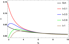
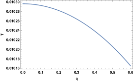
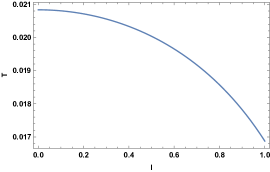
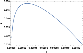
the Hawking temperature related to is determined to be:
| (37) |
and is plotted in Figs. (2) and 3 for different values of , and . Moreover, the horizon area is plainly calculated as which gives the black hole entropy to be .
III WEAK DEFLECTION ANGLE OF AMCNS BLACK HOLE USING THE GAUSS-BONNET THEOREM
The deflection angle of a photon approaching the said black hole with the distance of closest approach corresponds to Virbhadra et al. (1998); Weinberg (1972); Lu and Xie (2019):
| (38) |
The condition is satisfied for weak lensing since the deflection angle will be too small Keeton and Petters (2005). As verges on the photon sphere, increases until it diverges, hence, giving rise to strong lensing. Considering the equatorial plane in which equation Eq. (16) reduces to the optical metric for null geodesics:
| (39) |
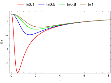
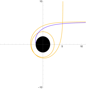
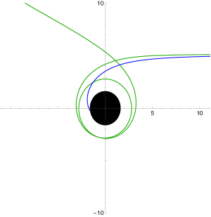
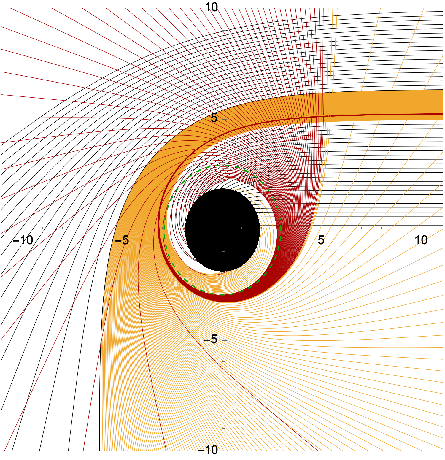
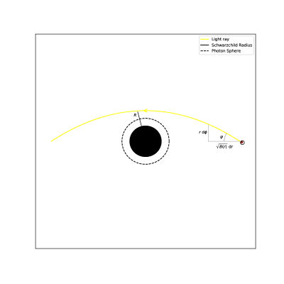
As mentioned above, the optical metric takes advantage of its geodesics for the topological effect that relates it to the Gauss-Bonnet theorem. The photon behaviors within the AMCHS black hole for a range of l values are illustrated in Figure 4. Subsequently, Figure 5 presents the paths followed by light rays as they orbit around the AMCHS black hole using the method defined in Gralla et al. (2019).
In that context, we delve deeper into the geodesics of the optical metric that governs the AMCNS black hole in Fig. 4. Notice the slightest difference in the light ray trajectory approaching from infinity towards the black hole that determines the fate of the light ray, an expected repercussion of the electric charge to starkly either pull the ray in or divert it around. Besides, an increase in is observed to retract the light rays more swiftly towards the black hole center. Extrapolating this further, Fig. 5 encapsulates the raytracing of the AMCNS metric. The abrupt coiling is more obvious in the myriad of light rays in this figure.

The Gaussian curvature is computed from the non-zero Christoffel symbols due to its proportionality where is the Ricci scalar and is found to be:
| (40) |
Employing the straight-line approximation for the impact parameter , the Gauss-Bonnet theorem suggests that Gibbons and Werner (2008); Kumaran and Övgün (2021):
| (41) |
where . Owing to the complexity of this calculation, the Gaussian curvature was reduced to and the integral was simplified by ignoring the higher-order terms . Thus, the deflection angle due to weak lensing for an asymptotic, magnetically charged, non-singular black hole is estimated to be:
| (42) |
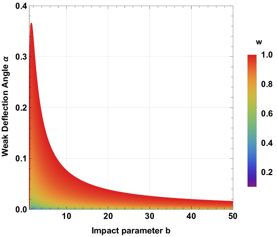
in the weak-field limit. Note that the mass function defined by Eq. (22) is employed here in the place of . From this result, the deflection angle is expected to change significantly because of the parameters that govern the black hole, reducing it to the case of a Schwarzschild black hole when , , and . This relation is depicted in Fig. 6.
Taking a look at this equation graphically, the deflection angle is seen to be vividly affected by and more intensely for . The ranges of values for and are chosen according to the acquirable potentialities of a charged particle in the black hole locale. The deviating curve shows that the deflection angle is more than the Schwarzschild case when there is an electric charge, and it keeps increasing as increases. The deceiving large contribution from is seemingly increasing the deflection angle.
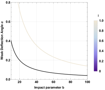
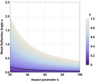
Therefore, the presence of the charge appears to be enhancing the deflection angle. This suggests that the distortions will be stronger, more evident, and could contain more information about the characteristics of the black hole’s structure and of the light source.
III.1 Weak Deflection Angle in dark matter medium
The presence of a medium significantly affects the dispersive properties of light rays compared to those in a vacuum. One such medium that is known to exist almost always is the one surrounded by dark matter. The observations from the Event Horizon Telescope of enormous dark matter halos around the black holes in the galactic centers. Its ability to engulf galaxies and to invade the interstellar and intergalactic media makes it a matter of inquisitivity. When surrounding a black hole, the extreme gravity experienced by the dark matter added to its already enduring gravitational impacts constitutes an important component of astrophysics that would greatly aid the gravitational lensing analyses.
To evaluate the consequences of dark matter on the deflection angle, the refractive index computed from the scatterers is defined as outlined in references Latimer (2013); Övgün (2019b, 2020):
| (43) |
In the given equation, represents the frequency of light. The term introduces a quantity denoted as , where denotes the mass density of the scattered particles of dark matter. The parameter is defined, where represents the charge of the scatterer in units of , and is a non-negative value. The terms of order and higher account for the polarizability of the dark matter particle. This expression presents the refractive index expected for an optically inactive medium. The term of order corresponds to a charged dark matter candidate, while corresponds to a neutral dark matter candidate. Additionally, a linear term in may be present if there exist parity and charge-parity asymmetries.
The line element in equation (16) can be reformulated using the optical metric as follows Crisnejo and Gallo (2018); Övgün (2019a); Javed et al. (2019):
| (44) |
As in the previous section, the weak deflection angle of an asymptotic, magnetically charged, non-singular black hole enveloped by dark matter can be expressed as:
| (45) |
In Figure 7, it is demonstrated that the deflection angle exhibits an upward trend as the parameter increases within the weak field limits, implying more dark matter activity engenders more distortions in the lensing profile. While it is not possible to predict how dark matter behaves around a black hole as opposed to the well-understood outer-galactic distribution, its fundamentality of augmenting the distortions, and by extension, the deflection angle, is unchanging.
IV ACCRETION DISK AND SHADOW CAST OF AMCNS BLACK HOLE
In this section, the shadow that is formed by a black hole that has a thin-accretion disk is examined. An accretion disk refers to the structure that arises from the gravitational pull of a central gravitating object on the adjacent matter like gas or dust Bambi (2012, 2013); Jaroszynski and Kurpiewski (1997); Gralla et al. (2019). As this matter moves toward the central object, it gains kinetic energy and generates a rapidly rotating disk around it. The temperature and density of the disk can cause it to emit radiation in different forms, such as X-rays, visible light, or radio waves. Accretion disks serve as an essential component in the development and progression of gravitating objects since they facilitate the transfer of mass and angular momentum.
When the accretion disk concurs with the lensing effect, produces the appearance of a shadow of a black hole. In essence, the phenomenon of gravitational lensing is the key factor that distinguishes the black hole shadow in the Newtonian case in contrast to that of the general-relativistic case, thus, exaggerating the shadow with the bending of light. The critical curve segregating the capture orbits and the scattering orbits forms the shadow with a geometrically thick, optically thin region filled with emitters (that either spiral into the black hole or swerve away from it) and is associated with a distant, homogeneous, isotropic emission ring. The former property is important while talking about an emission region since the intensity takes a dip that is coincident with the shadow, making it observable through this strong visual signature. The size of the shadow is mainly determined by the inherent parameters of the black hole, and its contour is shape-shifting owing to the instability in the orbits of the light rays from the photon sphere. For a distant observer, the shadow appears as a dark, two-dimensional disk, which is illuminated by its bright and uniform surroundings.
For the line element given by Eq. (16), introducing the function such that:
| (46) |
which is equivalent to the effective potential for photon motion Perlick and Tsupko (2022). Not that according to line element in 16, . Eq. (47) can be rearranged and rewritten as:
| (47) |
where, the impact parameter yet again. This equation is analogous to the traditional energy-conservation law described for one-dimensional motion in classical mechanics:
| (48) |
with taking the place of the temporal variable and the effective potential displaying its dependence on , and by extension, . This is also known as the orbit equation.
To determine the circular trajectories, the equations and can be solved. For a light ray approaching the center, if there exists a point at which it turns back around to exit the orbit after the ray reaches the minimum radius , then the condition needs to be complied with, yielding the orbit equation to be:
| (49) |
This relation between the constant of motion and instigates the following relationship:
| (50) |
which in turn yields:
| (51) |
Say, a static observer located at a radial coordinate shoots one light ray to the past. The dimensionless quantity is identified in terms of the cotangent to be:
| (52) |
as represented by Fig. 8 to be the measurable angle between the light ray and the radial coordinate which is directed towards the point of closest approach. It is termed as the angular radius of the shadow.
Here, the light ray approaching the circular (with radius ), unstable photon orbits asymptotically is oriented to the past, and so is the shadow’s boundary curve. In the limit where where , the above expression can be rewritten as:
| (54) |
This implies:
| (55) |
In the pursuit of calculating for the metric in Eq. (16) next, it is essential to realize that both and should simultaneously be zero. Differentiating Eq. (47), all terms vanish following the conditions except the third term acquired from the parentheses which are equated to zero resulting in:
| (56) |
The range of values that can take is extensive inferring that there could be multiple photon orbits – stable and unstable, existing together, with the light rays oscillating and spiraling respectively – impinging on the construction of the black hole shadow. For , the shadow can be determined for any distance, small or large, in a static, spherically-symmetric, asymptotically-flat spacetime with from Eq. (54) by:
| (57) |
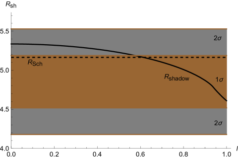
In the numerical plot depicted in Fig. 9, the radius of the black hole’s shadow () is calculated for different values of for asymptotically flat case , and ). It is intriguing to observe the exponential and inverse relationship exhibited by , irrespective of the range within which the parameters vary. In Fig. 9, the upper limits of are presented based on EHT observations. According to the confidence level (C.L.) Vagnozzi et al. (2023), the upper limit for is .
IV.1 Spherically infalling accretion
In this section, we explore the model of spherically free-falling accretion around AMCNS black hole from an infinite distance. The approach described in references Jaroszynski and Kurpiewski (1997); Bambi (2012) is employed for this investigation. By utilizing this method, we can generate a realistic representation of the shadow produced by the accretion disk. However, in reality, the actual image of the black hole cannot be observed as a discernible boundary in the universe. Additionally, employing a static accretion-disk model is not feasible due to the presence of a dynamic accretion disk surrounding the black hole. This dynamic disk also generates synchrotron emission as part of the accretion process. To accomplish this, our initial focus is on studying the specific intensity observed at the frequency of the photon by solving the following integral along the path of light:
| (58) |
We should mention that represents the impact parameter, corresponds to the emissivity per unit volume, represents the infinitesimal proper length, and denotes the frequency of the emitted photon. In this context, we introduce the redshift factor for the accretion in free-fall using the following definition:
| (59) |
The equation provided states that the 4-velocity of the photon is represented by , while the 4-velocity of the distant observer is denoted as . Furthermore, represents the 4-velocity of the infalling accretion:
| (60) |
By utilizing , one can derive the constants of motion and for the photons.
| (61) |
It is worth noting that the sign of indicates whether the photon approaches or deviates away from the black hole. Based on this, the redshift factor and proper distance can be expressed as follows:
| (62) |
and
| (63) |
Next, we restrict our analysis to monochromatic emission, where the specific emissivity is considered with a rest-frame frequency .
| (64) |
Subsequently, the intensity equation, given in equation (58), can be expressed as follows:
| (65) |
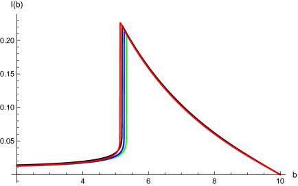
To analyze the shadow created by the thin accretion disk around the black hole, we begin by numerically solving the aforementioned equation. This numerical calculation is performed using the Einsteinpy library Bapat et al. (2021) and the Mathematica notebook package Okyay and Övgün (2022), which have also been utilized in previous studies Chakhchi et al. (2022); Kuang and Övgün (2022); Uniyal et al. (2023a); Pantig and Övgün (2023). The integration of the flux reveals the impact of the parameter on the specific intensity observed by a distant observer for an in-falling accretion. The corresponding results are presented in Figures 10, 11, and 12.
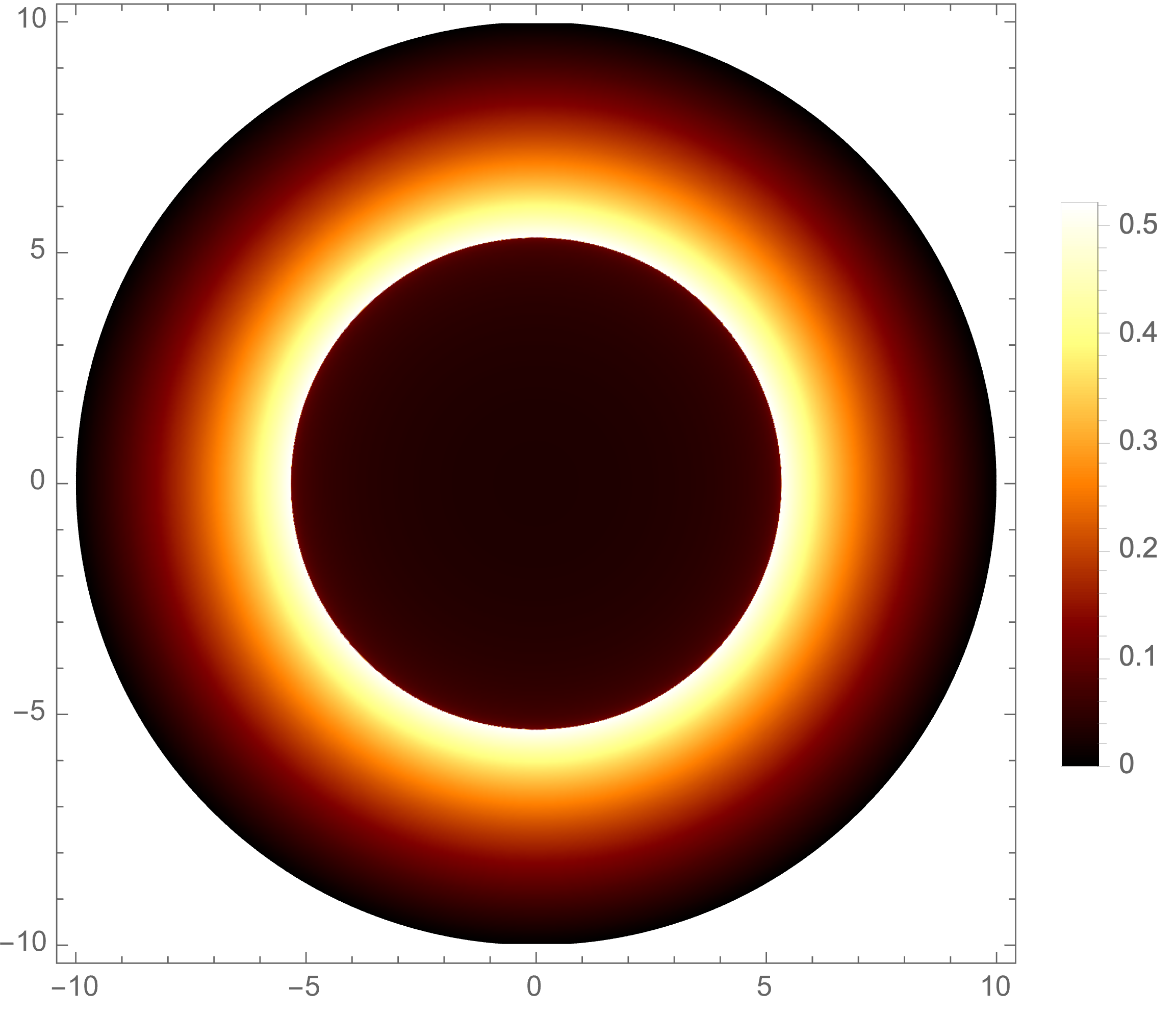
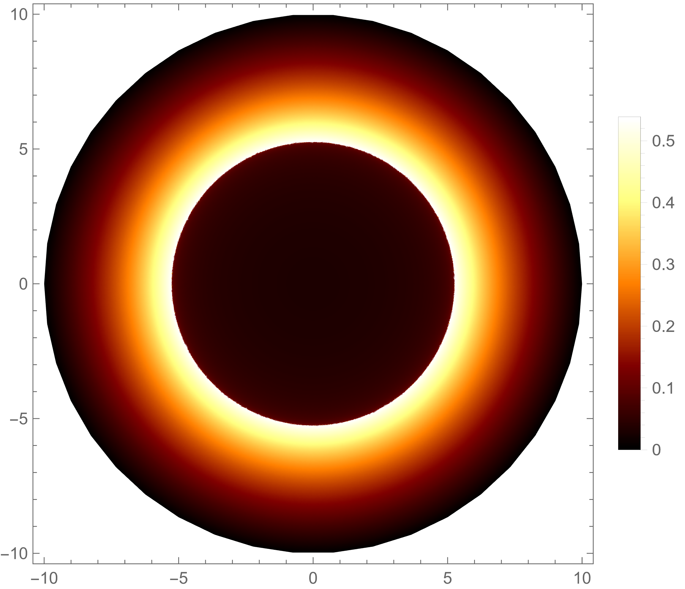

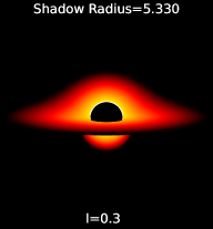
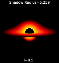

The figures in Fig. 11, and 12 show the intensity plots and stereographic projections of the AMCNS black hole described following the method of Bambi (2013); Jaroszynski and Kurpiewski (1997); Gralla et al. (2019). The intensity plot shows the smooth transition between the layers in the journey directed away from the event horizon. The sharpness in every photon band in Fig. 12 indicates the effect of the parameters , , and appearing to be brighter.
The difference in the appearance of the shadow sizes between the three images in Fig. 11 is hard to miss. The emissivity from the innermost photon orbit is seen to get brighter as increases. Consequently, the size of dark shadow region appears to be decreasing. Numerically speaking, Fig. 10 depicts how small yet non-trivial this difference is. The shadow outline seen in the images of Fig. 12 clearly exemplifies that the manifestation of additional inner-orbits of photons proportionally increasing with instigates the peak intensity to grow.
When compared with the shadow of a Schwarzschild black hole, the crucial factor that brings about a striking distinction between them is singularity. The Schwarzschild black hole is singular at its center meaning that it is a point of infinite density and zero volume. Among all the properties of a black hole that are disturbed by this (such as curvature, geometry, density profile, etc.), the one that is sizably impacted is the event horizon which is a mathematical construct that assumes the black hole is a point singularity. For a non-singular black hole, this assumption does not hold; in that case, the event horizon becomes an apparent boundary beyond which light cannot escape to infinity, but can still escape to some finite distance. This leads the non-singular black hole to have a smaller event horizon than the Schwarzschild black hole, which in turn explains the former’s smaller shadow size.
In summary, any entity that skirts around a black hole rendering a time-dependent appearance of the shadow will inexorably give rise to distortions, big or small, contingent on its characteristics. Also, the singularity at the center of a black hole can cause its space-time geometry to curve more bringing about a wider event horizon and a bigger shadow size. On the other hand, a non-singular black hole would have a smoother geometry and a smaller horizon that results in a smaller shadow size. Furthermore, dark matter intensifies the extent of distortions because of dispersion.
V BOUNDING THE GREYBODY FACTORS OF AMCNS BLACK HOLE
The equivalence of black holes to black bodies inspires curiosity about their relationship. This section is devoted to inspecting that correlation. A black body is an idealized object that absorbs all radiation that strikes it and emits radiation without incurring any loss at all wavelengths and at the maximum frequency; for a given spectrum, although the wavelength is dependent on temperature, its efficiency is 100%. Whereas, black holes absorb all radiation and matter inside the event horizon and emit Hawking radiation that is dependent on the mass of the black hole preserving the quantum information of the engulfed particles Hawking (1975); Akhmedov et al. (2006). While the gravity field and the matter encompassing a black hole deteriorates its energy eventually impairing the Hawking radiation emitted by the black hole from being fully efficient, its resemblance to a pure black body at its horizon, when isolated (resulting from quantum effects), is impeccable.
The deteriorating aspects of a radiating black hole are given by the greybody factor: the nomenclature underlines the departure from the black body behavior. It is a function of frequency and angular momentum that typifies the degree of deviation in the emission spectrum of a black hole from a perfect black body spectrum. The main culprit for this digression is the scattering of the radiation by the geometry of the black hole itself relating to the captured/radiated particles that fall back into the extreme force. This causes the spectrum emitted by the black hole to deviate and can be observed as the greybody factor Maldacena and Strominger (1997); Harmark et al. (2010); Rincón and Panotopoulos (2018); Rincón and Santos (2020); Panotopoulos and Rincón (2018, 2017); Klebanov and Mathur (1997); Liu et al. (2022); Fernando (2005); Konoplya et al. (2019); Javed et al. (2022d, e); Yang et al. (2023); Javed et al. (2022f); Mangut et al. (2023); Kanzi et al. (2023); Al-Badawi et al. (2022); Al-Badawi (2022); Al-Badawi et al. (2023).
By the scattering of a wave packet off a black hole, the greybody factor can be determined with the help of the classical Klein-Gordon equation – the Schrödinger-like equation that governs the modes for a wave function relating the position of an electron to its wave amplitude is written as:
| (66) |
where, is commonly known as the tortoise coordinate. Its purpose is to evolve to infinity in a manner that counters the singularity of the metric under scrutiny. The time of an object looming towards the event horizon in the constructed system of coordinates grows to infinity… so does but at a rate that is appropriate. Mathematically:
| (67) |
and the potential for the azimuthal quantum number specifying the mode can accordingly be formulated as:
| (68) |
This embodies the potential energy of the particle when there is an external force/field. The information about the wavefunction, the bound and scattering states, etc. can be begotten from this quantity.
Assuming that the energy of the particles emitted by the black hole falls in the range to for a given wave frequency , let be a positive function that obeys and when . To find the lower bound, the condition must be satisfied, implying that and the transmission probability is deduced as follows Visser (1999); Boonserm and Visser (2008); Boonserm et al. (2018):
| (69) | ||||
This expression for offers insight into the probability of a particle with a specific energy and angular momentum escaping the black hole and being detected at infinity. Yet again, is the radius of the event horizon of the black hole: it directly affects the details of the emitted radiation spectrum. Because of the intricacy of solving for the polynomial, we procure numerically.
The term describes the discrete robustness of quantum mechanics in general relativity by providing a measure of the angular momentum carried by the particles that the black hole emits. Also called the angular momentum quantum number, the value that takes says quite a lot about the emitted particles and spectrum:
-
•
insinuates that the emitted particles have zero angular momentum and are moving in a direction away from the black hole. The probability of a particle escaping the black hole in this case is maximum at low energies and it decreases as the energy of the particle increases. The spectrum of emitted radiation for the particles in this state is typically dominated by low-energy photons.
-
•
insinuates that the emitted particles have some angular momentum and are moving in a circular orbit around the black hole. The probability of a particle escaping the black hole in this case is maximum at intermediate energies and it decreases at both low and high energies. The spectrum of emitted radiation for the particles in this state typically peaks at intermediate energy.
Therefore, the value of particularizes the detailed shape of the spectrum of the radiation that a black hole emits, granting information about the features of the black hole itself. The graphical representation of the results acquired for and is presented in Figs. 13, 13(a) and 13(b) respectively for an AMCNS black hole.
Plotted to show the variation of the potential in terms of the radial coordinate for varying , Fig. 13(a) is perceived to show a negative intercept that rises to positive until a certain value before falling again when . However, for , Fig. 13(b) has a negative trough that briskly rises with to positive.
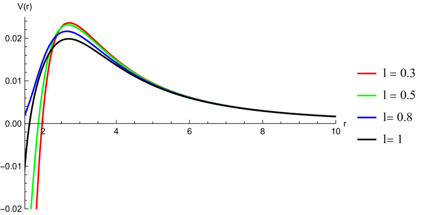
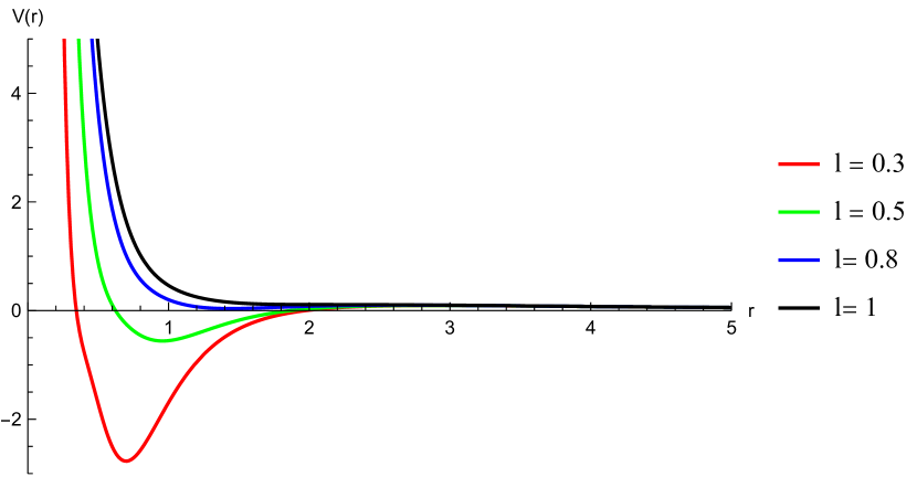
Fig. 14 illustrates the variation of the Transmission probability in terms of the frequency for different values of for an AMCNS black hole when . While the graph traits of all cases in Fig. 14(a) are analogous to each other with the same probability, a closer look at the ascension in the frequency range of infers that any and every variation (even the ones of the smallest magnitude) in the parameters of a black hole gives rise to an innate frequency.
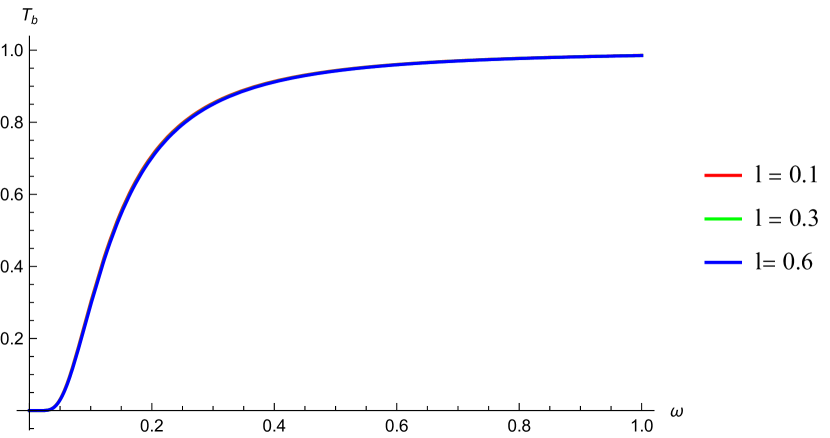
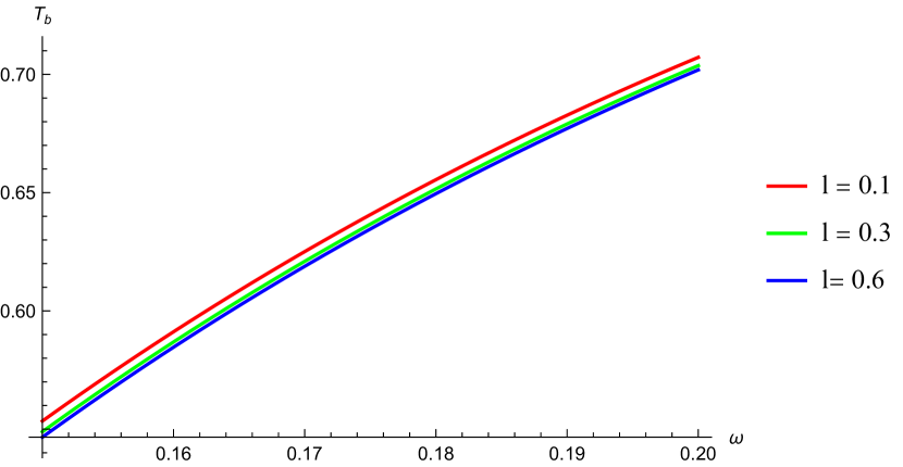
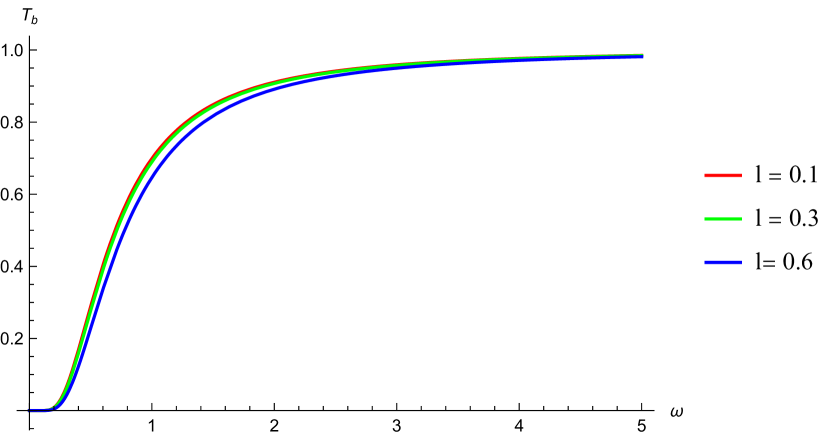
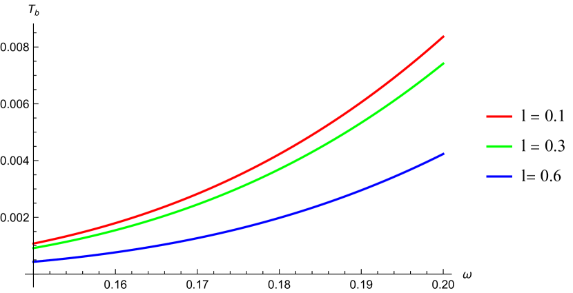
Fig. 15 illustrates the variation of the Transmission probability in terms of the frequency for different values of for an AMCNS black hole when . In Fig. 15(a), the probability of transmission of each case is discrete from the others and is noticed to be higher for lower values of , converging to unity as increases. The offsetting of every different in Fig. 15(b) is highly conspicuous attributable to the factor of angular momentum that prevails. Recalling that is a length-scale parameter, the decrease in with increasing can be explained by the inverse proportionality exhibited by frequency with respect to wavelength.
Nevertheless, the overall nature of the AMCNS black hole plots is adequately comparable to that of the Schwarzschild case and to Figs. 2 and 5 in in which the author handles a regular Hayward black hole.
VI CONCLUSION
In this article, we have attempted to analyze the astrophysics of an asymptotic, magnetically-charged, non-singular black hole. o find its solution, we commenced with the Euler-Lagrange equation for nonlinear electrodynamics and applied it to the Hayward metric through the trace of the energy-momentum tensor. Establishing its connection to the energy density eased us in uncovering the mass function and, with additional computations, the metric function of the AMCNS black hole.
This illation was then employed in the Gauss-Bonnet theorem and modified with the Gibbons and Werner method to obtain the weak deflection angle of the AMCNS black hole. This is done with the aim of examining the black hole’s gravitational field, its intrinsic attributes such as mass, spin, etc., the nature of the light bending, and, ultimately, the validity of Einstein’s theory deeper. These help us comprehend the dynamics of black holes better and prepares Observational Astrophysicists on what to or not to expect. The deflection angle that was obtained was observed to be vastly variant for the AMCNS black hole with an increase that is triggered by its governing parameters.
We then proceeded to calculate the effects of the dark matter medium on the deflection angle. Numerous theoretical and experimental endeavors are adopted to bridge the gap between physics and astrophysics; incorporating the consequences of dark matter majorly subsidizes that. Dark matter plays a key role in the intensified regime of black holes accreting and jets launching. The dark matter medium was perceived to increase the deflection more, and for the AMCNS balc hole, the slightest drop in the refractive index generated an immense upshot.
The greybody factor was then investigated using the Schrödinger-like equation. The potential and the transmission probability were derived for the AMCNS black hole and were plotted against a Schwarzschild black hole. One can discern the sizable differences in each of the curves for every case of the azimuthal quantum number.
Finally, the black hole shadow was probed for the AMCNS case. Although many parameters affect the shadow size, the factors assumed here for this particular black hole display highly distinguished traits, making the black hole fairly distinctive from a Schwarzschild black hole. With the assistance of the Euler-Lagrange equation once again, the critical curve and the shadow’s angular radius were determined. They were scrutinized thoroughly with stereographic projections; the singularity at the center of the Schwarzschild black hole curves and distorts its spacetime geometry more than that of a non-singular black hole, therefore, having a larger horizon and shadow size. The smoother spacetime geometry of the AMCNS black hole gives it a relatively smaller horizon and shadow size.
Meticulous methodologies of maximal parametric inclusiveness facilitate us in refining our comprehension of gravitational lensing. The distortions that every black hole produces offer so much information about the source of the light rays along with the black hole, which in turn motivates us to come up with new hypotheses that could polish and perfect our perception: our future work is directed toward the same. we intend to gather as many contributing factors that affect our grasp of black hole theories as possible and enhance them, no matter how complex it is, so that both theoretical and observational astrophysics can use them as a resource for improvement. We hope to attain ways that could minimize our assumptions like zero spin, staticity, spherical symmetry, and so many other constraints, and deal with the black hole realistically instead to the greatest degree feasible.
Acknowledgements.
A. Ö. would like to acknowledge the contribution of the COST Action CA18108 - Quantum gravity phenomenology in the multi-messenger approach (QG-MM) and the COST Action CA21106 - COSMIC WISPers in the Dark Universe: Theory, astrophysics and experiments (CosmicWISPers). A. Ö. is funded by the Scientific and Technological Research Council of Turkey (TUBITAK).References
- Montgomery et al. (2009) Colin Montgomery, Wayne Orchiston, and Ian Whittingham, “Michell, Laplace and the origin of the black hole concept,” Journal of Astronomical History and Heritage 12, 90–96 (2009).
- de Laplace (1799) P.S. de Laplace, Exposition du systeme du monde. Seconde edition revue et augmentee (Crapelet, 1799).
- Einstein (1916) Albert Einstein, “The Foundation of the General Theory of Relativity,” Annalen Phys. 49, 769–822 (1916).
- Schwarzschild (1916) Karl Schwarzschild, “On the gravitational field of a mass point according to Einstein’s theory,” Sitzungsber. Preuss. Akad. Wiss. Berlin (Math. Phys. ) 1916, 189–196 (1916), arXiv:physics/9905030 .
- Nordström (1918) G. Nordström, “On the Energy of the Gravitation field in Einstein’s Theory,” Koninklijke Nederlandse Akademie van Wetenschappen Proceedings Series B Physical Sciences 20, 1238–1245 (1918).
- Akiyama et al. (2019) Kazunori Akiyama et al. (Event Horizon Telescope), “First M87 Event Horizon Telescope Results. I. The Shadow of the Supermassive Black Hole,” Astrophys. J. Lett. 875, L1 (2019), arXiv:1906.11238 [astro-ph.GA] .
- Akiyama et al. (2022) Kazunori Akiyama et al. (Event Horizon Telescope), “First Sagittarius A* Event Horizon Telescope Results. I. The Shadow of the Supermassive Black Hole in the Center of the Milky Way,” Astrophys. J. Lett. 930, L12 (2022).
- Kocherlakota et al. (2021a) Prashant Kocherlakota et al. (Event Horizon Telescope), “Constraints on black-hole charges with the 2017 EHT observations of M87*,” Phys. Rev. D 103, 104047 (2021a), arXiv:2105.09343 [gr-qc] .
- Vagnozzi et al. (2023) Sunny Vagnozzi, Rittick Roy, Yu-Dai Tsai, Luca Visinelli, Misba Afrin, Alireza Allahyari, Parth Bambhaniya, Dipanjan Dey, Sushant G Ghosh, Pankaj S. Joshi, Kimet Jusufi, Mohsen Khodadi, Rahul Kumar Walia, Ali Övgün, and Cosimo Bambi, “Horizon-scale tests of gravity theories and fundamental physics from the event horizon telescope image of sagittarius a*,” Classical and Quantum Gravity (2023), arXiv:2205.07787 [gr-qc] .
- Penrose (1965) Roger Penrose, “Gravitational collapse and space-time singularities,” Phys. Rev. Lett. 14, 57–59 (1965).
- Hawking (1975) S. W. Hawking, “Particle Creation by Black Holes,” Commun. Math. Phys. 43, 199–220 (1975), [Erratum: Commun.Math.Phys. 46, 206 (1976)].
- Bardeen (1968) James M Bardeen, “Non-singular general-relativistic gravitational collapse,” Proceedings of International Conference GR5 (Tbilisi, USSR, 1968) , 174 (1968).
- Carleo et al. (2022) Amodio Carleo, Gaetano Lambiase, and Ali Övgün, “Non-linear Electrodynamics in Blandford-Znajeck Energy Extraction,” (2022), 10.1002/andp.202200635, arXiv:2210.11162 [gr-qc] .
- Hayward (2006) Sean A. Hayward, “Formation and evaporation of regular black holes,” Phys. Rev. Lett. 96, 031103 (2006), arXiv:gr-qc/0506126 .
- Luminet (1979) J. P. Luminet, “Image of a spherical black hole with thin accretion disk,” Astron. Astrophys. 75, 228–235 (1979).
- Falcke et al. (2000) Heino Falcke, Fulvio Melia, and Eric Agol, “Viewing the shadow of the black hole at the galactic center,” Astrophys. J. Lett. 528, L13 (2000), arXiv:astro-ph/9912263 .
- Bronzwaer and Falcke (2021) Thomas Bronzwaer and Heino Falcke, “The Nature of Black Hole Shadows,” Astrophys. J. 920, 155 (2021), arXiv:2108.03966 [astro-ph.HE] .
- Narayan et al. (2019) Ramesh Narayan, Michael D. Johnson, and Charles F. Gammie, “The Shadow of a Spherically Accreting Black Hole,” Astrophys. J. Lett. 885, L33 (2019), arXiv:1910.02957 [astro-ph.HE] .
- Pantig et al. (2023) Reggie C. Pantig, Ali Övgün, and Durmuş Demir, “Testing symmergent gravity through the shadow image and weak field photon deflection by a rotating black hole using the M87∗ and Sgr. results,” Eur. Phys. J. C 83, 250 (2023), arXiv:2208.02969 [gr-qc] .
- Çimdiker et al. (2021) İrfan Çimdiker, Durmuş Demir, and Ali Övgün, “Black hole shadow in symmergent gravity,” Phys. Dark Univ. 34, 100900 (2021), arXiv:2110.11904 [gr-qc] .
- Rayimbaev et al. (2023) Javlon Rayimbaev, Reggie C. Pantig, Ali Övgün, Ahmadjon Abdujabbarov, and Durmuş Demir, “Quasiperiodic oscillations, weak field lensing and shadow cast around black holes in Symmergent gravity,” Annals of Physics (2023), 10.1016/j.aop.2023.169335, arXiv:2206.06599 [gr-qc] .
- Ghosh et al. (2021) Sushant G. Ghosh, Rahul Kumar, and Shafqat Ul Islam, “Parameters estimation and strong gravitational lensing of nonsingular Kerr-Sen black holes,” JCAP 03, 056 (2021), arXiv:2011.08023 [gr-qc] .
- Allahyari et al. (2020) Alireza Allahyari, Mohsen Khodadi, Sunny Vagnozzi, and David F. Mota, “Magnetically charged black holes from non-linear electrodynamics and the Event Horizon Telescope,” JCAP 02, 003 (2020), arXiv:1912.08231 [gr-qc] .
- Bambi et al. (2019) Cosimo Bambi, Katherine Freese, Sunny Vagnozzi, and Luca Visinelli, “Testing the rotational nature of the supermassive object M87* from the circularity and size of its first image,” Phys. Rev. D 100, 044057 (2019), arXiv:1904.12983 [gr-qc] .
- Kocherlakota et al. (2021b) Prashant Kocherlakota, Luciano Rezzolla, Heino Falcke, et al. (EHT Collaboration), “Constraints on black-hole charges with the 2017 eht observations of m87*,” Phys. Rev. D 103, 104047 (2021b).
- Övgün et al. (2018) Ali Övgün, İzzet Sakallı, and Joel Saavedra, “Shadow cast and Deflection angle of Kerr-Newman-Kasuya spacetime,” JCAP 10, 041 (2018), arXiv:1807.00388 [gr-qc] .
- Övgün and Sakallı (2020) Ali Övgün and İzzet Sakallı, “Testing generalized Einstein–Cartan–Kibble–Sciama gravity using weak deflection angle and shadow cast,” Class. Quant. Grav. 37, 225003 (2020), arXiv:2005.00982 [gr-qc] .
- Övgün et al. (2020) Ali Övgün, İzzet Sakallı, Joel Saavedra, and Carlos Leiva, “Shadow cast of noncommutative black holes in Rastall gravity,” Mod. Phys. Lett. A 35, 2050163 (2020), arXiv:1906.05954 [hep-th] .
- Kuang and Övgün (2022) Xiao-Mei Kuang and Ali Övgün, “Strong gravitational lensing and shadow constraint from M87* of slowly rotating Kerr-like black hole,” (2022), arXiv:2205.11003 [gr-qc] .
- Kumaran and Övgün (2022) Yashmitha Kumaran and Ali Övgün, “Deflection Angle and Shadow of the Reissner–Nordström Black Hole with Higher-Order Magnetic Correction in Einstein-Nonlinear-Maxwell Fields,” Symmetry 14, 2054 (2022), arXiv:2210.00468 [gr-qc] .
- Mustafa et al. (2022) Ghulam Mustafa, Farruh Atamurotov, Ibrar Hussain, Sanjar Shaymatov, and Ali Övgün, “Shadows and gravitational weak lensing by the Schwarzschild black hole in the string cloud background with quintessential field*,” Chin. Phys. C 46, 125107 (2022), arXiv:2207.07608 [gr-qc] .
- Okyay and Övgün (2022) Mert Okyay and Ali Övgün, “Nonlinear electrodynamics effects on the black hole shadow, deflection angle, quasinormal modes and greybody factors,” JCAP 01, 009 (2022), arXiv:2108.07766 [gr-qc] .
- Atamurotov et al. (2023) Farruh Atamurotov, Ibrar Hussain, Ghulam Mustafa, and Ali Övgün, “Weak deflection angle and shadow cast by the charged-Kiselev black hole with cloud of strings in plasma*,” Chin. Phys. C 47, 025102 (2023).
- Abdikamalov et al. (2019) Askar B. Abdikamalov, Ahmadjon A. Abdujabbarov, Dimitry Ayzenberg, Daniele Malafarina, Cosimo Bambi, and Bobomurat Ahmedov, “Black hole mimicker hiding in the shadow: Optical properties of the metric,” Phys. Rev. D 100, 024014 (2019), arXiv:1904.06207 [gr-qc] .
- Abdujabbarov et al. (2016) Ahmadjon Abdujabbarov, Bakhtinur Juraev, Bobomurat Ahmedov, and Zdeněk Stuchlík, “Shadow of rotating wormhole in plasma environment,” Astrophys. Space Sci. 361, 226 (2016).
- Atamurotov and Ahmedov (2015) Farruh Atamurotov and Bobomurat Ahmedov, “Optical properties of black hole in the presence of plasma: shadow,” Phys. Rev. D 92, 084005 (2015), arXiv:1507.08131 [gr-qc] .
- Papnoi et al. (2014) Uma Papnoi, Farruh Atamurotov, Sushant G. Ghosh, and Bobomurat Ahmedov, “Shadow of five-dimensional rotating Myers-Perry black hole,” Phys. Rev. D 90, 024073 (2014), arXiv:1407.0834 [gr-qc] .
- Abdujabbarov et al. (2013) Ahmadjon Abdujabbarov, Farruh Atamurotov, Yusuf Kucukakca, Bobomurat Ahmedov, and Ugur Camci, “Shadow of Kerr-Taub-NUT black hole,” Astrophys. Space Sci. 344, 429–435 (2013), arXiv:1212.4949 [physics.gen-ph] .
- Atamurotov et al. (2013) Farruh Atamurotov, Ahmadjon Abdujabbarov, and Bobomurat Ahmedov, “Shadow of rotating non-Kerr black hole,” Phys. Rev. D 88, 064004 (2013).
- Cunha and Herdeiro (2018) Pedro V. P. Cunha and Carlos A. R. Herdeiro, “Shadows and strong gravitational lensing: a brief review,” Gen. Rel. Grav. 50, 42 (2018), arXiv:1801.00860 [gr-qc] .
- Gralla et al. (2019) Samuel E. Gralla, Daniel E. Holz, and Robert M. Wald, “Black Hole Shadows, Photon Rings, and Lensing Rings,” Phys. Rev. D 100, 024018 (2019), arXiv:1906.00873 [astro-ph.HE] .
- Belhaj et al. (2021) A. Belhaj, H. Belmahi, M. Benali, W. El Hadri, H. El Moumni, and E. Torrente-Lujan, “Shadows of 5D black holes from string theory,” Phys. Lett. B 812, 136025 (2021), arXiv:2008.13478 [hep-th] .
- Belhaj et al. (2020) A. Belhaj, M. Benali, A. El Balali, H. El Moumni, and S. E. Ennadifi, “Deflection angle and shadow behaviors of quintessential black holes in arbitrary dimensions,” Class. Quant. Grav. 37, 215004 (2020), arXiv:2006.01078 [gr-qc] .
- Konoplya (2019) R. A. Konoplya, “Shadow of a black hole surrounded by dark matter,” Phys. Lett. B 795, 1–6 (2019), arXiv:1905.00064 [gr-qc] .
- Wei et al. (2019) Shao-Wen Wei, Yuan-Chuan Zou, Yu-Xiao Liu, and Robert B. Mann, “Curvature radius and Kerr black hole shadow,” JCAP 08, 030 (2019), arXiv:1904.07710 [gr-qc] .
- Ling et al. (2021) Ru Ling, Hong Guo, Hang Liu, Xiao-Mei Kuang, and Bin Wang, “Shadow and near-horizon characteristics of the acoustic charged black hole in curved spacetime,” Phys. Rev. D 104, 104003 (2021), arXiv:2107.05171 [gr-qc] .
- Kumar et al. (2020) Rahul Kumar, Sushant G. Ghosh, and Anzhong Wang, “Gravitational deflection of light and shadow cast by rotating Kalb-Ramond black holes,” Phys. Rev. D 101, 104001 (2020), arXiv:2001.00460 [gr-qc] .
- Kumar and Ghosh (2017) Rahul Kumar and Sushant G. Ghosh, “Accretion onto a noncommutative geometry inspired black hole,” European Physical Journal C 77, 577 (2017), arXiv:1703.10479 [gr-qc] .
- Cunha et al. (2017) Pedro V. P. Cunha, Carlos A. R. Herdeiro, Burkhard Kleihaus, Jutta Kunz, and Eugen Radu, “Shadows of Einstein–dilaton–Gauss–Bonnet black holes,” Phys. Lett. B 768, 373–379 (2017), arXiv:1701.00079 [gr-qc] .
- Cunha et al. (2016a) Pedro V. P. Cunha, Carlos A. R. Herdeiro, Eugen Radu, and Helgi F. Runarsson, “Shadows of Kerr black holes with and without scalar hair,” Int. J. Mod. Phys. D 25, 1641021 (2016a), arXiv:1605.08293 [gr-qc] .
- Cunha et al. (2016b) P. V. P. Cunha, J. Grover, C. Herdeiro, E. Radu, H. Runarsson, and A. Wittig, “Chaotic lensing around boson stars and Kerr black holes with scalar hair,” Phys. Rev. D 94, 104023 (2016b), arXiv:1609.01340 [gr-qc] .
- Zakharov (2014) Alexander F. Zakharov, “Constraints on a charge in the Reissner-Nordström metric for the black hole at the Galactic Center,” Phys. Rev. D 90, 062007 (2014), arXiv:1407.7457 [gr-qc] .
- Tsukamoto (2018) Naoki Tsukamoto, “Black hole shadow in an asymptotically-flat, stationary, and axisymmetric spacetime: The Kerr-Newman and rotating regular black holes,” Phys. Rev. D 97, 064021 (2018), arXiv:1708.07427 [gr-qc] .
- Chakhchi et al. (2022) L. Chakhchi, H. El Moumni, and K. Masmar, “Shadows and optical appearance of a power-Yang-Mills black hole surrounded by different accretion disk profiles,” Phys. Rev. D 105, 064031 (2022).
- Li et al. (2020a) Peng-Cheng Li, Minyong Guo, and Bin Chen, “Shadow of a Spinning Black Hole in an Expanding Universe,” Phys. Rev. D 101, 084041 (2020a), arXiv:2001.04231 [gr-qc] .
- Pantig and Övgün (2023) Reggie C. Pantig and Ali Övgün, “Testing dynamical torsion effects on the charged black hole’s shadow, deflection angle and greybody with M87* and Sgr. A* from EHT,” Annals Phys. 448, 169197 (2023), arXiv:2206.02161 [gr-qc] .
- Pantig et al. (2022) Reggie C. Pantig, Leonardo Mastrototaro, Gaetano Lambiase, and Ali Övgün, “Shadow, lensing, quasinormal modes, greybody bounds and neutrino propagation by dyonic ModMax black holes,” Eur. Phys. J. C 82, 1155 (2022), arXiv:2208.06664 [gr-qc] .
- Lobos and Pantig (2022) Nikko John Leo S. Lobos and Reggie C. Pantig, “Generalized extended uncertainty principle black holes: Shadow and lensing in the macro- and microscopic realms,” Physics 4, 1318–1330 (2022).
- Uniyal et al. (2023a) Akhil Uniyal, Reggie C. Pantig, and Ali Övgün, “Probing a non-linear electrodynamics black hole with thin accretion disk, shadow, and deflection angle with M87* and Sgr A* from EHT,” Phys. Dark Univ. 40, 101178 (2023a), arXiv:2205.11072 [gr-qc] .
- Övgün et al. (2023) Ali Övgün, Reggie C. Pantig, and Ángel Rincón, “4D scale-dependent Schwarzschild-AdS/dS black holes: study of shadow and weak deflection angle and greybody bounding,” Eur. Phys. J. Plus 138, 192 (2023), arXiv:2303.01696 [gr-qc] .
- Uniyal et al. (2023b) Akhil Uniyal, Sayan Chakrabarti, Reggie C. Pantig, and Ali Övgün, “Nonlinearly charged black holes: Shadow and Thin-accretion disk,” (2023b), arXiv:2303.07174 [gr-qc] .
- Panotopoulos et al. (2021) Grigoris Panotopoulos, Ángel Rincón, and Ilidio Lopes, “Orbits of light rays in scale-dependent gravity: Exact analytical solutions to the null geodesic equations,” Phys. Rev. D 103, 104040 (2021), arXiv:2104.13611 [gr-qc] .
- Panotopoulos and Rincon (2022) Grigoris Panotopoulos and Angel Rincon, “Orbits of light rays in (1+2)-dimensional Einstein–power–Maxwell gravity: Exact analytical solution to the null geodesic equations,” Annals Phys. 443, 168947 (2022), arXiv:2206.03437 [gr-qc] .
- Khodadi and Lambiase (2022) Mohsen Khodadi and Gaetano Lambiase, “Probing Lorentz symmetry violation using the first image of Sagittarius A: Constraints on standard model extension coefficients,” Phys. Rev. D 106, 104050 (2022), arXiv:2206.08601 [gr-qc] .
- Khodadi et al. (2021) Mohsen Khodadi, Gaetano Lambiase, and David F. Mota, “No-hair theorem in the wake of Event Horizon Telescope,” JCAP 09, 028 (2021), arXiv:2107.00834 [gr-qc] .
- Meng et al. (2023) Yuan Meng, Xiao-Mei Kuang, Xi-Jing Wang, and Jian-Pin Wu, “Shadow revisiting and weak gravitational lensing with Chern-Simons modification,” (2023), 10.1016/j.physletb.2023.137940, arXiv:2305.04210 [gr-qc] .
- Pantig and Övgün (2022a) Reggie C. Pantig and Ali Övgün, “Dehnen halo effect on a black hole in an ultra-faint dwarf galaxy,” JCAP 08, 056 (2022a), arXiv:2202.07404 [astro-ph.GA] .
- Pantig and Övgün (2022b) Reggie C. Pantig and Ali Övgün, “Black hole in quantum wave dark matter,” Fortsch. Phys. 2022, 2200164 (2022b), arXiv:2210.00523 [gr-qc] .
- Pantig (2023) Reggie C. Pantig, “Constraining a one-dimensional wave-type gravitational wave parameter through the shadow of M87* via Event Horizon Telescope,” (2023), arXiv:2303.01698 [gr-qc] .
- Wang et al. (2021) Mingzhi Wang, Songbai Chen, and Jiliang Jing, “Effect of gravitational wave on shadow of a Schwarzschild black hole,” Eur. Phys. J. C 81, 509 (2021), arXiv:1908.04527 [gr-qc] .
- Roy and Chakrabarti (2020) Rittick Roy and Sayan Chakrabarti, “Study on black hole shadows in asymptotically de Sitter spacetimes,” Phys. Rev. D 102, 024059 (2020), arXiv:2003.14107 [gr-qc] .
- Konoplya (2021) R. A. Konoplya, “Black holes in galactic centers: Quasinormal ringing, grey-body factors and Unruh temperature,” Phys. Lett. B 823, 136734 (2021), arXiv:2109.01640 [gr-qc] .
- Anjum et al. (2023) Arshia Anjum, Misba Afrin, and Sushant G. Ghosh, “Astrophysical consequences of dark matter for photon orbits and shadows of supermassive black holes,” (2023), arXiv:2301.06373 [gr-qc] .
- Hou et al. (2018) Xian Hou, Zhaoyi Xu, Ming Zhou, and Jiancheng Wang, “Black hole shadow of Sgr A∗ in dark matter halo,” JCAP 07, 015 (2018), arXiv:1804.08110 [gr-qc] .
- Lambiase et al. (2023) Gaetano Lambiase, Reggie C. Pantig, Dhruba Jyoti Gogoi, and Ali Övgün, “Investigating the Connection between Generalized Uncertainty Principle and Asymptotically Safe Gravity in Black Hole Signatures through Shadow and Quasinormal Modes,” (2023), arXiv:2304.00183 [gr-qc] .
- Shaikh (2022) Rajibul Shaikh, “Testing black hole mimickers with the Event Horizon Telescope image of Sagittarius A∗,” (2022), 10.1093/mnras/stad1383, arXiv:2208.01995 [gr-qc] .
- Shaikh et al. (2022) Rajibul Shaikh, Suvankar Paul, Pritam Banerjee, and Tapobrata Sarkar, “Shadows and thin accretion disk images of the -metric,” Eur. Phys. J. C 82, 696 (2022), arXiv:2105.12057 [gr-qc] .
- Shaikh et al. (2019) Rajibul Shaikh, Prashant Kocherlakota, Ramesh Narayan, and Pankaj S. Joshi, “Shadows of spherically symmetric black holes and naked singularities,” Mon. Not. Roy. Astron. Soc. 482, 52–64 (2019), arXiv:1802.08060 [astro-ph.HE] .
- Shaikh (2019) Rajibul Shaikh, “Black hole shadow in a general rotating spacetime obtained through Newman-Janis algorithm,” Phys. Rev. D 100, 024028 (2019), arXiv:1904.08322 [gr-qc] .
- Shaikh and Joshi (2019) Rajibul Shaikh and Pankaj S. Joshi, “Can we distinguish black holes from naked singularities by the images of their accretion disks?” JCAP 10, 064 (2019), arXiv:1909.10322 [gr-qc] .
- Shaikh et al. (2021) Rajibul Shaikh, Kunal Pal, Kuntal Pal, and Tapobrata Sarkar, “Constraining alternatives to the Kerr black hole,” Mon. Not. Roy. Astron. Soc. 506, 1229–1236 (2021), arXiv:2102.04299 [gr-qc] .
- Rahaman et al. (2021) Farook Rahaman, Tuhina Manna, Rajibul Shaikh, Somi Aktar, Monimala Mondal, and Bidisha Samanta, “Thin accretion disks around traversable wormholes,” Nucl. Phys. B 972, 115548 (2021), arXiv:2110.09820 [gr-qc] .
- Virbhadra and Ellis (2000) K. S. Virbhadra and George F. R. Ellis, “Schwarzschild black hole lensing,” Phys. Rev. D 62, 084003 (2000), arXiv:astro-ph/9904193 .
- Virbhadra and Ellis (2002) K. S. Virbhadra and G. F. R. Ellis, “Gravitational lensing by naked singularities,” Phys. Rev. D 65, 103004 (2002).
- Adler and Virbhadra (2022) Stephen L. Adler and K. S. Virbhadra, “Cosmological constant corrections to the photon sphere and black hole shadow radii,” (2022), arXiv:2205.04628 [gr-qc] .
- Bozza et al. (2001) V. Bozza, S. Capozziello, G. Iovane, and G. Scarpetta, “Strong field limit of black hole gravitational lensing,” Gen. Rel. Grav. 33, 1535–1548 (2001), arXiv:gr-qc/0102068 .
- Bozza (2002) V. Bozza, “Gravitational lensing in the strong field limit,” Phys. Rev. D 66, 103001 (2002), arXiv:gr-qc/0208075 .
- Perlick (2004) Volker Perlick, “On the Exact gravitational lens equation in spherically symmetric and static space-times,” Phys. Rev. D 69, 064017 (2004), arXiv:gr-qc/0307072 .
- He et al. (2020) Guansheng He, Xia Zhou, Zhongwen Feng, Xueling Mu, Hui Wang, Weijun Li, Chaohong Pan, and Wenbin Lin, “Gravitational deflection of massive particles in Schwarzschild-de Sitter spacetime,” Eur. Phys. J. C 80, 835 (2020).
- Virbhadra (2022a) K. S. Virbhadra, “Compactness of supermassive dark objects at galactic centers,” (2022a), arXiv:2204.01792 [gr-qc] .
- Virbhadra (2022b) K. S. Virbhadra, “Distortions of images of Schwarzschild lensing,” (2022b), arXiv:2204.01879 [gr-qc] .
- Gibbons and Werner (2008) G. W. Gibbons and M. C. Werner, “Applications of the Gauss-Bonnet theorem to gravitational lensing,” Class. Quant. Grav. 25, 235009 (2008), arXiv:0807.0854 [gr-qc] .
- Övgün et al. (2022) Ali Övgün, Yashmitha Kumaran, Wajiha Javed, and Jameela Abbas, “Effect of Horndeski theory on weak deflection angle using the Gauss–Bonnet theorem,” Int. J. Geom. Meth. Mod. Phys. 19, 2250192 (2022).
- Kumaran and Övgün (2021) Yashmitha Kumaran and Ali Övgün, “Deriving weak deflection angle by black holes or wormholes using Gauss-Bonnet theorem,” Turk. J. Phys. 45, 247–267 (2021), arXiv:2111.02805 [gr-qc] .
- Javed et al. (2021) Wajiha Javed, Jameela Abbas, Yashmitha Kumaran, and Ali Övgün, “Weak deflection angle by asymptotically flat black holes in Horndeski theory using Gauss-Bonnet theorem,” Int. J. Geom. Meth. Mod. Phys. 18, 2150003 (2021), arXiv:2102.02812 [gr-qc] .
- Kumaran and Övgün (2020) Yashmitha Kumaran and Ali Övgün, “Weak Deflection Angle of Extended Uncertainty Principle Black Holes,” Chin. Phys. C 44, 025101 (2020), arXiv:1905.11710 [gr-qc] .
- Övgün (2018) Ali Övgün, “Light deflection by Damour-Solodukhin wormholes and Gauss-Bonnet theorem,” Phys. Rev. D 98, 044033 (2018), arXiv:1805.06296 [gr-qc] .
- Övgün (2019a) A. Övgün, “Weak field deflection angle by regular black holes with cosmic strings using the Gauss-Bonnet theorem,” Phys. Rev. D 99, 104075 (2019a), arXiv:1902.04411 [gr-qc] .
- Övgün (2019b) Ali Övgün, “Deflection Angle of Photons through Dark Matter by Black Holes and Wormholes Using Gauss–Bonnet Theorem,” Universe 5, 115 (2019b), arXiv:1806.05549 [physics.gen-ph] .
- Javed et al. (2019) Wajiha Javed, Rimsha Babar, and Alï Övgün, “Effect of the dilaton field and plasma medium on deflection angle by black holes in Einstein-Maxwell-dilaton-axion theory,” Phys. Rev. D 100, 104032 (2019), arXiv:1910.11697 [gr-qc] .
- Werner (2012) M. C. Werner, “Gravitational lensing in the Kerr-Randers optical geometry,” Gen. Rel. Grav. 44, 3047–3057 (2012), arXiv:1205.3876 [gr-qc] .
- Ishihara et al. (2016) Asahi Ishihara, Yusuke Suzuki, Toshiaki Ono, Takao Kitamura, and Hideki Asada, “Gravitational bending angle of light for finite distance and the Gauss-Bonnet theorem,” Phys. Rev. D 94, 084015 (2016), arXiv:1604.08308 [gr-qc] .
- Ono et al. (2017) Toshiaki Ono, Asahi Ishihara, and Hideki Asada, “Gravitomagnetic bending angle of light with finite-distance corrections in stationary axisymmetric spacetimes,” Phys. Rev. D 96, 104037 (2017), arXiv:1704.05615 [gr-qc] .
- Li and Övgün (2020) Zonghai Li and Ali Övgün, “Finite-distance gravitational deflection of massive particles by a Kerr-like black hole in the bumblebee gravity model,” Phys. Rev. D 101, 024040 (2020), arXiv:2001.02074 [gr-qc] .
- Li et al. (2020b) Zonghai Li, Guodong Zhang, and Ali Övgün, “Circular Orbit of a Particle and Weak Gravitational Lensing,” Phys. Rev. D 101, 124058 (2020b), arXiv:2006.13047 [gr-qc] .
- Belhaj et al. (2022) A. Belhaj, H. Belmahi, M. Benali, and H. Moumni El, “Light Deflection by Rotating Regular Black Holes with a Cosmological Constant,” (2022), arXiv:2204.10150 [gr-qc] .
- Pantig and Övgün (2022c) Reggie C. Pantig and Ali Övgün, “Dark matter effect on the weak deflection angle by black holes at the center of Milky Way and M87 galaxies,” Eur. Phys. J. C 82, 391 (2022c), arXiv:2201.03365 [gr-qc] .
- Javed et al. (2023) Wajiha Javed, Mehak Atique, Reggie C. Pantig, and Ali Övgün, “Weak Deflection Angle, Hawking Radiation and Greybody Bound of Reissner-Nordström Black Hole Corrected by Bounce Parameter,” Symmetry 15, 148 (2023), arXiv:2301.01855 [gr-qc] .
- Javed et al. (2022a) Wajiha Javed, Mehak Atique, Reggie C. Pantig, and Ali Övgün, “Weak lensing, Hawking radiation and greybody factor bound by a charged black holes with non-linear electrodynamics corrections,” International Journal of Geometric Methods in Modern Physics , 2350040 (2022a).
- Javed et al. (2022b) Wajiha Javed, Sibgha Riaz, Reggie C. Pantig, and Ali Övgün, “Weak gravitational lensing in dark matter and plasma mediums for wormhole-like static aether solution,” Eur. Phys. J. C 82, 1057 (2022b), arXiv:2212.00804 [gr-qc] .
- Javed et al. (2022c) Wajiha Javed, Hafsa Irshad, Reggie C. Pantig, and Ali Övgün, “Weak Deflection Angle by Kalb–Ramond Traversable Wormhole in Plasma and Dark Matter Mediums,” Universe 8, 599 (2022c), arXiv:2211.07009 [gr-qc] .
- Breton (2003) Nora Breton, “Born-Infeld black hole in the isolated horizon framework,” Phys. Rev. D 67, 124004 (2003), arXiv:hep-th/0301254 .
- Hendi (2013) S. H. Hendi, “Asymptotic Reissner-Nordstroem black holes,” Annals Phys. 333, 282–289 (2013), arXiv:1405.5359 [gr-qc] .
- Kruglov (2015) S. I. Kruglov, “Nonlinear electrodynamics and black holes,” Int. J. Geom. Meth. Mod. Phys. 12, 1550073 (2015), arXiv:1504.03941 [physics.gen-ph] .
- Kruglov (2016a) S. I. Kruglov, “Asymptotic Reissner-Nordström solution within nonlinear electrodynamics,” Phys. Rev. D 94, 044026 (2016a), arXiv:1608.04275 [gr-qc] .
- Kruglov (2016b) S. I. Kruglov, “Nonlinear arcsin-electrodynamics and asymptotic Reissner-Nordström black holes,” Annalen Phys. 528, 588–596 (2016b), arXiv:1607.07726 [gr-qc] .
- Kruglov (2017) S. I. Kruglov, “Black hole as a magnetic monopole within exponential nonlinear electrodynamics,” Annals Phys. 378, 59–70 (2017), arXiv:1703.02029 [gr-qc] .
- Övgün (2021) A. Övgün, “Black hole with confining electric potential in scalar-tensor description of regularized 4-dimensional Einstein-Gauss-Bonnet gravity,” Phys. Lett. B 820, 136517 (2021), arXiv:2105.05035 [gr-qc] .
- Ali and Saifullah (2019) Askar Ali and Khalid Saifullah, “Asymptotic magnetically charged non-singular black hole and its thermodynamics,” Phys. Lett. B 792, 276–283 (2019), arXiv:1904.05727 [gr-qc] .
- Bera et al. (2020) Avijit Bera, Subir Ghosh, and Bibhas Ranjan Majhi, “Hawking radiation in a non-covariant frame: the Jacobi metric approach,” Eur. Phys. J. Plus 135, 670 (2020), arXiv:1909.12607 [gr-qc] .
- Gibbons (2016) G. W. Gibbons, “The Jacobi-metric for timelike geodesics in static spacetimes,” Class. Quant. Grav. 33, 025004 (2016), arXiv:1508.06755 [gr-qc] .
- Chanda et al. (2017) Sumanto Chanda, G. W. Gibbons, and Partha Guha, “Jacobi-Maupertuis-Eisenhart metric and geodesic flows,” J. Math. Phys. 58, 032503 (2017), arXiv:1612.00375 [math-ph] .
- Das et al. (2017) Praloy Das, Ripon Sk, and Subir Ghosh, “Motion of charged particle in Reissner–Nordström spacetime: a Jacobi-metric approach,” Eur. Phys. J. C 77, 735 (2017), arXiv:1609.04577 [gr-qc] .
- Srinivasan and Padmanabhan (1999) K. Srinivasan and T. Padmanabhan, “Particle production and complex path analysis,” Phys. Rev. D 60, 024007 (1999), arXiv:gr-qc/9812028 .
- Robinson and Wilczek (2005) Sean P. Robinson and Frank Wilczek, “A Relationship between Hawking radiation and gravitational anomalies,” Phys. Rev. Lett. 95, 011303 (2005), arXiv:gr-qc/0502074 .
- Iso et al. (2006) Satoshi Iso, Hiroshi Umetsu, and Frank Wilczek, “Hawking radiation from charged black holes via gauge and gravitational anomalies,” Phys. Rev. Lett. 96, 151302 (2006), arXiv:hep-th/0602146 .
- Majhi (2010) Bibhas Ranjan Majhi, Quantum Tunneling in Black Holes, Ph.D. thesis, Calcutta U. (2010), arXiv:1110.6008 [gr-qc] .
- Virbhadra et al. (1998) K. S. Virbhadra, D. Narasimha, and S. M. Chitre, “Role of the scalar field in gravitational lensing,” Astron. Astrophys. 337, 1–8 (1998), arXiv:astro-ph/9801174 .
- Weinberg (1972) Steven Weinberg, Gravitation and Cosmology: Principles and Applications of the General Theory of Relativity (John Wiley and Sons, New York, 1972).
- Lu and Xie (2019) Xu Lu and Yi Xie, “Weak and strong deflection gravitational lensing by a renormalization group improved Schwarzschild black hole,” Eur. Phys. J. C 79, 1016 (2019).
- Keeton and Petters (2005) Charles R. Keeton and A. O. Petters, “Formalism for testing theories of gravity using lensing by compact objects. I. Static, spherically symmetric case,” Phys. Rev. D 72, 104006 (2005), arXiv:gr-qc/0511019 .
- Latimer (2013) David C. Latimer, “Dispersive Light Propagation at Cosmological Distances: Matter Effects,” Phys. Rev. D 88, 063517 (2013), arXiv:1308.1112 [hep-ph] .
- Övgün (2020) Ali Övgün, “Weak Deflection Angle of Black-bounce Traversable Wormholes Using Gauss-Bonnet Theorem in the Dark Matter Medium,” Turk. J. Phys. 44, 465–471 (2020), arXiv:2011.04423 [gr-qc] .
- Crisnejo and Gallo (2018) Gabriel Crisnejo and Emanuel Gallo, “Weak lensing in a plasma medium and gravitational deflection of massive particles using the Gauss-Bonnet theorem. A unified treatment,” Phys. Rev. D 97, 124016 (2018), arXiv:1804.05473 [gr-qc] .
- Bambi (2012) Cosimo Bambi, “A code to compute the emission of thin accretion disks in non-Kerr space-times and test the nature of black hole candidates,” Astrophys. J. 761, 174 (2012), arXiv:1210.5679 [gr-qc] .
- Bambi (2013) Cosimo Bambi, “Can the supermassive objects at the centers of galaxies be traversable wormholes? The first test of strong gravity for mm/sub-mm very long baseline interferometry facilities,” Phys. Rev. D 87, 107501 (2013), arXiv:1304.5691 [gr-qc] .
- Jaroszynski and Kurpiewski (1997) M. Jaroszynski and A. Kurpiewski, “Optics near kerr black holes: spectra of advection dominated accretion flows,” Astron. Astrophys. 326, 419 (1997), arXiv:astro-ph/9705044 .
- Perlick and Tsupko (2022) Volker Perlick and Oleg Yu. Tsupko, “Calculating black hole shadows: Review of analytical studies,” Phys. Rept. 947, 1–39 (2022), arXiv:2105.07101 [gr-qc] .
- Bapat et al. (2021) Shreyas Bapat et al., “einsteinpy/einsteinpy: Einsteinpy 0.4.0,” (2021).
- Akhmedov et al. (2006) Emil T. Akhmedov, Valeria Akhmedova, and Douglas Singleton, “Hawking temperature in the tunneling picture,” Phys. Lett. B 642, 124–128 (2006), arXiv:hep-th/0608098 .
- Maldacena and Strominger (1997) Juan Martin Maldacena and Andrew Strominger, “Black hole grey body factors and d-brane spectroscopy,” Phys. Rev. D 55, 861–870 (1997), arXiv:hep-th/9609026 .
- Harmark et al. (2010) Troels Harmark, Jose Natario, and Ricardo Schiappa, “Greybody Factors for d-Dimensional Black Holes,” Adv. Theor. Math. Phys. 14, 727–794 (2010), arXiv:0708.0017 [hep-th] .
- Rincón and Panotopoulos (2018) Ángel Rincón and Grigoris Panotopoulos, “Greybody factors and quasinormal modes for a nonminimally coupled scalar field in a cloud of strings in (2+1)-dimensional background,” Eur. Phys. J. C 78, 858 (2018), arXiv:1810.08822 [gr-qc] .
- Rincón and Santos (2020) Ángel Rincón and Victor Santos, “Greybody factor and quasinormal modes of Regular Black Holes,” Eur. Phys. J. C 80, 910 (2020), arXiv:2009.04386 [gr-qc] .
- Panotopoulos and Rincón (2018) Grigoris Panotopoulos and Angel Rincón, “Greybody factors for a minimally coupled scalar field in three-dimensional Einstein-power-Maxwell black hole background,” Phys. Rev. D 97, 085014 (2018), arXiv:1804.04684 [hep-th] .
- Panotopoulos and Rincón (2017) Grigoris Panotopoulos and Ángel Rincón, “Greybody factors for a minimally coupled massless scalar field in Einstein-Born-Infeld dilaton spacetime,” Phys. Rev. D 96, 025009 (2017), arXiv:1706.07455 [hep-th] .
- Klebanov and Mathur (1997) Igor R. Klebanov and Samir D. Mathur, “Black hole grey body factors and absorption of scalars by effective strings,” Nucl. Phys. B 500, 115–132 (1997), arXiv:hep-th/9701187 .
- Liu et al. (2022) Dong Liu, Yi Yang, Ali Övgün, Zheng-Wen Long, and Zhaoyi Xu, “Quasinormal Modes and Greybody Bounds of Rotating Black Holes in a Dark Matter Halo,” (2022), arXiv:2204.11563 [gr-qc] .
- Fernando (2005) Sharmanthie Fernando, “Greybody factors of charged dilaton black holes in 2 + 1 dimensions,” Gen. Rel. Grav. 37, 461–481 (2005), arXiv:hep-th/0407163 .
- Konoplya et al. (2019) R. A. Konoplya, A. Zhidenko, and A. F. Zinhailo, “Higher order WKB formula for quasinormal modes and grey-body factors: recipes for quick and accurate calculations,” Class. Quant. Grav. 36, 155002 (2019), arXiv:1904.10333 [gr-qc] .
- Javed et al. (2022d) Wajiha Javed, Sibgha Riaz, and Ali Övgün, “Weak Deflection Angle and Greybody Bound of Magnetized Regular Black Hole,” Universe 8, 262 (2022d), arXiv:2205.02229 [gr-qc] .
- Javed et al. (2022e) Wajiha Javed, Muhammad Aqib, and Ali Övgün, “Effect of the magnetic charge on weak deflection angle and greybody bound of the black hole in Einstein-Gauss-Bonnet gravity,” Phys. Lett. B 829, 137114 (2022e), arXiv:2204.07864 [gr-qc] .
- Yang et al. (2023) Yi Yang, Dong Liu, Ali Övgün, Zheng-Wen Long, and Zhaoyi Xu, “Probing hairy black holes caused by gravitational decoupling using quasinormal modes and greybody bounds,” Phys. Rev. D 107, 064042 (2023), arXiv:2203.11551 [gr-qc] .
- Javed et al. (2022f) Wajiha Javed, Iqra Hussain, and Ali Övgün, “Weak deflection angle of Kazakov–Solodukhin black hole in plasma medium using Gauss–Bonnet theorem and its greybody bonding,” Eur. Phys. J. Plus 137, 148 (2022f), arXiv:2201.09879 [gr-qc] .
- Mangut et al. (2023) M. Mangut, H. Gürsel, S. Kanzi, and İ. Sakallı, “Probing the Lorentz Invariance Violation via Gravitational Lensing and Analytical Eigenmodes of Perturbed Slowly Rotating Bumblebee Black Holes,” (2023), 10.3390/universe9050225, arXiv:2305.10815 [gr-qc] .
- Kanzi et al. (2023) Sara Kanzi, İzzet Sakallı, and Behnam Pourhassan, “Superradiant (In)stability, Greybody Radiation, and Quasinormal Modes of Rotating Black Holes in non-linear Maxwell f (R) Gravity,” (2023), 10.3390/sym15040873, arXiv:2301.03866 [hep-th] .
- Al-Badawi et al. (2022) Ahmad Al-Badawi, Sara Kanzi, and İzzet Sakallı, “Greybody radiation of scalar and Dirac perturbations of NUT black holes,” Eur. Phys. J. Plus 137, 94 (2022), arXiv:2111.15005 [gr-qc] .
- Al-Badawi (2022) Ahmad Al-Badawi, “Greybody factor and perturbation of a Schwarzschild black hole with string clouds and quintessence,” Gen. Rel. Grav. 54, 11 (2022), arXiv:2201.09106 [gr-qc] .
- Al-Badawi et al. (2023) Ahmad Al-Badawi, Sara Kanzi, and İzzet Sakallı, “Fermionic and bosonic greybody factors as well as quasinormal modes for charged Taub NUT black holes,” Annals Phys. 452, 169294 (2023), arXiv:2203.04140 [hep-th] .
- Visser (1999) Matt Visser, “Some general bounds for 1-D scattering,” Phys. Rev. A 59, 427–438 (1999), arXiv:quant-ph/9901030 .
- Boonserm and Visser (2008) Petarpa Boonserm and Matt Visser, “Bounding the greybody factors for Schwarzschild black holes,” Phys. Rev. D 78, 101502 (2008), arXiv:0806.2209 [gr-qc] .
- Boonserm et al. (2018) Petarpa Boonserm, Tritos Ngampitipan, and Pitayuth Wongjun, “Greybody factor for black holes in dRGT massive gravity,” Eur. Phys. J. C 78, 492 (2018), arXiv:1705.03278 [gr-qc] .