Tree-Regularized Bayesian Latent Class Analysis for Improving Weakly Separated Dietary Pattern Subtyping in Small-Sized Subpopulations

Abstract

Dietary patterns synthesize multiple related diet components, which can be used by nutrition researchers to examine diet-disease relationships. Latent class models (LCMs) have been used to derive dietary patterns from dietary intake assessment, where each class profile represents the probabilities of exposure to a set of diet components. However, LCM-derived dietary patterns can exhibit strong similarities, or weak separation, resulting in numerical and inferential instabilities that challenge scientific interpretation. This issue is exacerbated in small-sized subpopulations. To address these issues, we provide a simple solution that empowers LCMs to improve dietary pattern estimation. We develop a tree-regularized Bayesian LCM that shares statistical strength between dietary patterns to make better estimates using limited data. This is achieved via a Dirichlet diffusion tree process that specifies a prior distribution for the unknown tree over classes. Dietary patterns that share proximity to one another in the tree are shrunk towards ancestral dietary patterns a priori, with the degree of shrinkage varying across pre-specified food groups. Using dietary intake data from the Hispanic Community Health Study/Study of Latinos, we apply the proposed approach to a sample of $496$ US adults of South American ethnic background to identify and compare dietary patterns.

Keywords: Dirichlet diffusion tree process; Dimension reduction; Tree-structured shrinkage; Model-based clustering; Nutritional epidemiology.

1 Introduction

1.1 Motivation

Dietary patterns refer to the quantities, proportions, variety, or combination of different foods, drinks, and nutrients in diets, and the frequency with which they are consumed (Dietary Guidelines Advisory Committee, 2020). Dietary patterns have been studied extensively in nutrition epidemiology to serve as potentially important predictors for health outcomes (The US Burden of Disease Collaborators, 2018). Understanding the heterogeneity of dietary consumption behaviors not only provides vital insights into relating diet with chronic diseases and mortality, but also helps tailor nutritional interventions to subgroups with distinct dietary patterns. Twenty-four-hour dietary recalls are a diet assessment tool that evaluates individual foods or nutrients consumed within the past 24-hours. While analysis of dietary behaviors can be conducted on individual foods or nutrients, many nutritionists argue for a holistic approach because foods are not consumed in isolation and nutrients have synergistic effects (Kant, 2004). Given the large number of foods to jointly analyze, dimension reduction techniques are often employed to understand dietary behaviors in a study population.

In our motivating application, 24-hour dietary recalls were distributed at baseline (2007-2011) to participants in the Hispanic Community Health Study/Study of Latinos (HCHS/SOL; LaVange et al., 2010). Due to the open-ended format of dietary recalls, a granular set of food items can be observed (e.g. 11,000 foods) and are often aggregated into servings per day of a smaller set of food items for analysis. Our study focuses on such multivariate categorical aggregated data accounting for food servings per day. When deriving dietary patterns based on these data, off-the-shelf dimension reduction methods face unique limitations. First, dietary patterns may only be distinguishable by a small subset of food items when culture and regionality are shared among participants (Mattei et al., 2016; Stephenson et al., 2020b). In other words, dietary patterns are weakly separated (Lubke and Muthén, 2007) from one another, meaning that the distances between patterns, jointly accounting for variation, are relatively small. For example, Sotres-Alvarez et al. (2010) analyzed pregnant women in North Carolina, where three dietary patterns were derived from intake data: prudent, health conscious Western, and hard core Western. Out of the 105 analyzed food items, only nine were distinguishable between the three patterns, implying that the remaining items shared indistinguishable behavior similarities. Although weak separation of dietary patterns may not cause estimation issues in large-sized cohorts, challenges may occur in small-sized populations (e.g., sample size $N<500$). For example, in the HCHS/SOL study, researchers have attempted to form subpopulations by ethnic background and study site to examine ethnic and regional heterogeneity in these participants (De Vito et al., 2022; Stephenson et al., 2020b). However, certain subpopulations were excluded due to limited sample sizes (e.g. Bronx participants of Central American background, $N=217$). In other HCHS/SOL subgroup analysis, these subpopulations were pooled across study sites into larger ethnic subpopulations (Maldonado et al., 2021). Excluding or pooling across small-sized subpopulations is ad hoc and less ideal because we may ignore demographic nuances that drive dietary behavior differences. The boundary of whether the sample size is large or small is often blurry. Size determination is relative to the degree of pattern separation in a particular data set. This calls for new adaptive methods that provide high quality inference across different sample sizes and are effective in cases where the sample size is small.

Second, the degree of dietary pattern separation may differ by major food groups that these food items are nutritionally nested under. For example, in the Sotres-Alvarez et al. (2010) study, the food items that shared similarities across different patterns belonged to some major food groups (e.g. sweets and fats), but differences were found amongst other major food groups (e.g. fruits and vegetables). Recognizing the distinct degrees of pattern separation by major food groups may improve dietary pattern estimation accuracy, and increase dietary pattern interpretability for nutrition researchers when a large number of food items are analyzed.

1.2 Existing Methods

Popular dimension reduction techniques to derive population-based dietary patterns include latent class models (LCMs; Park et al., 2020; Stephenson et al., 2020b), factor analysis (Engeset et al., 2015; Maldonado et al., 2021), and other clustering methods (Kant, 2004). In this paper, we focus on LCMs for the purpose of deriving dietary patterns and clustering individuals based on multivariate categorical food exposure level data. LCMs (Lazarsfeld, 1950; Goodman, 1974) partition the population into mutually exclusive subgroups (“latent classes”), within each of which individuals have similar dietary behaviors. Dietary patterns are defined as the probabilities of exposure to the individual food items, which are called item response probabilities or class profiles. Estimation of an LCM can be achieved in a Bayesian framework to allow flexible uncertainty quantification via posterior samples. Additionally, a Bayesian framework readily builds in a prior to encourage similarity between classes and incorporate additional food group information that will allow us to derive weakly separated dietary patterns in small-sized subpopulations.

Classical Bayesian LCMs assume item response probabilities are identical and independent a priori across classes and items. It can be challenging for the model to detect nuanced differences across dietary patterns. Patterns that are not well-separated coupled with small sample sizes often cause statistical issues of convergence failure, poor model fit, and poor empirical identifiability of classes with low prevalence (Lubke and Muthén, 2007; Park and Yu, 2018; Weller et al., 2020). One may argue for collapsing highly similar patterns into one. However, nuanced differences between patterns may be scientifically important. In addition, classical Bayesian LCMs do not take into account the varying degrees of separation amongst major food groups.

Prior studies such as robust profile clustering (RPC, Stephenson et al., 2020a) have used flexible models to improve dietary pattern analysis. RPC describes overall patterns (global clusters) by pooling across predefined subpopulations, and subpopulation-specific patterns (local clusters) that permit individual item response probability deviations from the overall patterns. However, RPC is not designed for weakly separated dietary patterns. It may still be constrained by sample size to effectively estimate patterns at the local level. For example, in each subpopulation considered in Stephenson et al. (2020b) where subpopulations sizes ranged from 300 to 3000, only one or two patterns were identified at the local level. This may be due to distinct but weakly-separated patterns that were inadvertently merged.

1.3 Main Contributions

We introduce a tree-regularized latent class model, a general framework to facilitate the sharing of information between classes to make better estimates of parameters using limited data. Our proposed model addresses weak separation for small sample sizes by (1) sharing statistical strength between classes guided by an unknown tree, and (2) accounting for varying degrees of shrinkage across major food groups. The proposed model uses a Dirichlet diffusion tree (DDT) process (Neal, 2003) as a fully probabilistic device to specify a prior distribution for the class profiles on the leaves of an unknown tree (hence termed “DDT-LCM”). Classes positioned closer on the tree exhibit more dietary pattern similarities. The degrees of separation by major food groups are modeled by group-specific diffusion variances.

Trees are intuitive and powerful for organizing and visualizing information about hierarchical relationship between entities in diverse scientific contexts, such as zoonotic diseases, hospital discharge codes, and text mining in fully probabilistic models (Li et al., 2023; Thomas et al., 2020; Blei et al., 2003; Zavitsanos et al., 2011; Weninger et al., 2012; Ghahramani et al., 2010; Roy et al., 2006; Yao et al., 2023). Sometimes we may know there is a true underlying hierarchy. For example, Li et al. (2023) incorporates known phylogenetic information among pathogens to study unobserved host origins of zoonotic diseases; Thomas et al. (2020) incorporates the hierarchical relationship among hospital discharge codes to boost the statistical power of detecting the association between fine particulate matter and granular cardiovascular outcomes. Even if no obvious hierarchy is present, we may expect certain component distributions to have similar parameters when modeling a complex multivariate distribution by a mixture model. For example, certain LCM-derived dietary patterns can share consumption similarities across many food items. Mixture models typically use independent priors over the component parameters that do not capture the hierarchical similarity structure. This leads to inefficient inference as more data is needed to estimate each of the model components (Neal, 2003; Knowles and Ghahramani, 2015). Our proposed method is designed to improve the inference by introducing and learning such a hierarchy among the classes in the framework of LCMs.

The rest of the paper is organized as follows. Section 2 defines tree-related terminologies to introduce the DDT framework and the DDT-LCM formulation. Section 3 derives the posterior sampling algorithm. Section 4 compares estimation performances of the proposed and alternative approaches via simulation studies. Section 5 applies DDT-LCM to a small-sized subgroup of the HCHS/SOL study to identify food consumption patterns of adults with South American ethnic background from 24-hour dietary recalls. Section 6 concludes with a brief discussion on study limitations and future directions.

2 Model Formulation

Throughout this paper, “major food group” refers to the pre-specified nutritional groups of food items, and “class” refers to individuals’ unknown dietary pattern memberships. For a positive integer $K$, we denote the set of positive integers up to $K$ by $[K]=\{1,\ldots,K\}$.

2.1 Latent Class Models

While LCMs are suitable for multivariate categorical responses with more than two levels, for ease of presentation, we focus on multivariate binary responses for this paper.

Assume that $J$ individual food items in our dataset belong to one of $G$ pre-specified major food groups (e.g., meat), where the $g$-th group consists of $J_{g}$ individual food items (e.g., poultry, pork, beef) and $J=\sum\limits_{g=1}^{G}J_{g}$ for $g\in[G]$. For example in Supplementary Table LABEL:tab:item_labels, the second major food group is “fruit” ($g=2$) which contains $J_{2}=6$ granular items with the third item being “citrus juice”.

We denote $\bm{Y}_{i}=(Y_{i,1,1},\ldots,Y_{i,1,J_{1}},\ldots,Y_{i,g,j},\ldots,Y_{i,G,1},\ldots,Y_{i,G,J_{G}})^{\top}\in\{0,1\}^{J}$ as the vector of observed binary responses for individual $i\in[N]$, such that $Y_{i,g,j}=1$ if the individual was exposed to the $j$-th item of the $g$-th major food group in the past 24 hours, $j\in[J_{g}]$, and $Y_{i,g,j}=0$ otherwise. Exposure to a food item within a major food group means the individual consumed this food at a predefined binary level. Let the $N\times J$ matrix $\bm{Y}=(\bm{Y}_{1},\ldots,\bm{Y}_{N})^{\top}$ collect the observed responses of all $N$ individuals. We assume that the $N$ individuals can be partitioned into $K$ latent classes and that individuals assigned to different classes have distinct exposure behaviors to the $J$ items. Let $Z_{i}$ be the class assignment indicator of the $i$-th individual and follow a categorical distribution with $P(Z_{i}=k)=\pi_{k},k\in[K]$, where $\bm{\pi}=(\pi_{1},\ldots,\pi_{K})\in\Delta_{K-1}$ is the class probability and $\Delta_{K-1}=\left\{\bm{r}\in[0,1]^{K}:\sum\limits_{k=1}^{K}r_{k}=1\right\}$ is the probability simplex. LCM assumes conditional independence, where item responses are independent given assignment to a latent class. LCM has the following generative process:

$$\begin{split}Z_{i}\mid\bm{\pi}&\sim\mathrm{Categorical}_{K}(\bm{\pi}),\\ Y_{i,g,j}\mid Z_{i}=k,\theta_{k,g,j}&\sim\mathrm{Bernoulli}\left(\theta_{k,g,j}\right),k\in[K],j\in[J_{g}],g\in[G].\end{split}$$ (1)

Here, $\theta_{k,g,j}$ is called the item response probability, or probability of exposure to food item $j$ in major food group $g$, in class $k$. In the $k$-th class, the vector of probabilities of exposure to the food items is represented as $\bm{\theta}_{k}=(\theta_{k,1,1},\ldots,\theta_{k,1,J_{1}},\ldots,\theta_{K,G,1},\ldots,\theta_{k,G,J_{G}})^{\top}$. This is also referenced as a class profile and characterizes the $k$-th dietary pattern of scientific interest. Concatenating all $\bm{\theta}_{k},k\in[K]$ by row, we obtain a $K\times J$ item response probability matrix $\bm{\Theta}$. The marginal probability of observing a particular response matrix $\bm{y}$ after integrating out the unobserved latent class assignments is $P(\bm{Y}=\bm{y}\mid\bm{\pi},\bm{\Theta})=$

$$\prod\limits_{i=1}^{N}\left[\sum\limits_{k=1}^{K}\pi_{k}P(\bm{Y}_{i}=\bm{y}_{i}\mid Z_{i}=k)\right]=\prod\limits_{i=1}^{N}\left[\sum\limits_{k=1}^{K}\pi_{k}\prod\limits_{g=1}^{G}\prod\limits_{j=1}^{J_{g}}(\theta_{k,g,j})^{Y_{i,g,j}}(1-\theta_{k,g,j})^{1-Y_{i,g,j}}\right].$$ (2)

2.2 Improper Rooted Binary Trees

A key component of the proposed framework is an improper rooted binary tree that encodes similarities between leaf entities (e.g., classes). An improper rooted binary tree is a directed graph where the root node has one child, all internal nodes have two children, and leaf nodes have no children.

Let ${\mathcal{T}}$ be an improper rooted binary tree with nodes $\mathcal{V}$, including leaf nodes $\mathcal{V}^{L}$ and internal nodes $\mathcal{V}^{I}=\mathcal{V}\setminus(\{u_{0}\}\cup\mathcal{V}^{L})$, where $u_{0}$ is the root node. An improper rooted binary tree with $|\mathcal{V}^{L}|=K$ leaf nodes contains $|\mathcal{V}^{I}|=K-1$ internal nodes and one root node, comprising a total of $|\mathcal{V}|=2K$ nodes. We will use $u\in\mathcal{V}$ to denote any node in the tree, and $v_{k}\in\mathcal{V}^{L},k\in[K]$ to denote a leaf node. For a node $u$ in the tree, we use $pa(u)$ to denote the parent of $u$, $a(u)$ the ancestors of $u$ including itself, and $d(u)$ the descendants of $u$ including itself. The ancestors of $u$ that are internal nodes are denoted as $a^{I}(u)=a(u)\setminus\{u_{0}\}$. The branch length between any two adjacent nodes $u$ and $u^{\prime}$ is denoted by $l_{u,u^{\prime}}$. The most recent common ancestor (MRCA) between any two nodes $u$ and $u^{\prime}$ (denoted as MRCA$(u,u^{\prime})$) is the most recent node of which $u$ and $u^{\prime}$ are descendants. Each node $u$ in the tree is associated with its own parameter, which may be a scalar or vector and we will refer to as “node parameter”, denoted as $\bm{\eta}_{u}$. In particular, the node parameter associated with a leaf node $v_{k}$ of the tree will be called “leaf parameter”, which is denoted as $\bm{\eta}_{k}$ for simplicity.

The left side of Figure 1 illustrates a tree with $K=4$ leaves. Among the $|\mathcal{V}|=8$ nodes, there are $|\mathcal{V}^{I}|=3$ internal nodes ($u_{1},u_{2}$ and $u_{3}$) as well as $|\mathcal{V}^{L}|=K=4$ leaf nodes ($v_{1},v_{2},v_{3}$ and $v_{4}$). In this tree, $pa(u_{3})=u_{2}$, $a(u_{3})=\{u_{0},u_{1},u_{2},u_{3}\}$, $a^{I}(u_{3})=\{u_{1},u_{2},u_{3}\}$, $d(u_{2})=\{u_{2},u_{3},v_{2},v_{3}\}$, and MRCA$(v_{1},v_{3})=u_{2}$. The root node and internal node parameters are $\bm{\eta}_{u_{0}},\bm{\eta}_{u_{1}},\bm{\eta}_{u_{2}}$ and $\bm{\eta}_{u_{3}}$, and the leaf parameters are $\bm{\eta}_{1},\bm{\eta}_{2},\bm{\eta}_{3}$ and $\bm{\eta}_{4}$.

Figure 1: Illustration of DDT-LCM with $K=4$ classes, and $J=10$ items categorized into $G=3$ major food groups shown in distinct colors. Right: In the observed data matrix for $N=13$ individuals, non-white cells indicate positive exposure to food items. The color corresponds to the item’s major food group. Middle: The dietary patterns are characterized by the item response probabilities. Left: A tree capturing the hierarchical relationship over the dietary patterns. In our data analysis, this tree is unknown and needs to be estimated.

2.3 Prior on the Unknown Tree for Dietary Patterns

2.3.1 Dirichlet Diffusion Trees

We provide a brief overview of the Dirichlet diffusion tree process (DDT; Neal, 2003; Knowles and Ghahramani, 2015) which will be used to specify a prior for the dietary patterns. Further details are provided in Supplementary Section S1.

The DDT process provides a family of nonparametric priors for distributions over exchangeable random quantities that arise from a latent branching process. DDT processes generalize Dirichlet processes by capturing the hierarchical structure present in complex distributions by means of a latent diffusion tree. A joint distribution is specified on improper rooted binary trees with a fixed number of leaves and Gaussian-distributed node parameters. It is also generalizable to fit non-Gaussian distributions through transformation (Knowles and Ghahramani, 2015). The DDT consists of two components: 1) tree topologies ${\mathcal{T}}$ and divergence times $\bm{t}$ on the unit time interval $[0,1]$, and 2) node parameters $\{\bm{\eta}_{u}\in\mathbb{R}^{J};u\in\mathcal{V}\}$ following Brownian motions along the branches given a tree topology and divergence times. Specifically, tree topologies and divergence times are simultaneously obtained from a branching process characterized by a divergence function $a(t),t\in[0,1]$. In subsequent simulations and applications, we choose $a(t)=c/(1-t)$, where $c>0$ is a “smoothness” hyperparameter. Larger $c$ values place higher prior weights on earlier divergence, leading to shallower trees and weaker prior dependence between different leaf parameters. Supplementary Section S1 provides details on the influence of hyperparameter $c$. Given a tree topology and divergence times, a $J$-dimensional node parameter is generated along the tree from a scaled Brownian motion starting at the root parameter $\bm{\eta}_{u_{0}}=\bm{0}_{J\times 1}$. Each element of a node parameter is independently scaled by a diffusion variance.

A sample drawn from the distribution over a $K$-leaf DDT, marginalized over all possible intermediate stochastic paths in the Brownian motions from root to leaves, consists of node parameters along with divergence times associated with a) one root node, b) $K-1$ internal nodes and c) $K$ leaf nodes: $\{(t_{u},\bm{\eta}_{u});u\in\mathcal{V}\}$. The non-root node parameters $\bm{\eta}=\{\bm{\eta}_{u};u\in\mathcal{V}\setminus\{u_{0}\}\}$ can be partitioned into two parts: $\bm{\eta}^{L}$ and $\bm{\eta}^{I}$. Here, $\bm{\eta}^{L}$ is a $K\times J$ matrix concatenating the leaf parameters by row so that the $k$-th row is $\bm{\eta}_{k}^{\top}$ (superscript $L$ is dropped for simplicity), and $\bm{\eta}^{I}$ is a $(K-1)\times J$ matrix concatenating the internal node parameters.

DDT provides a useful tool for constructing a prior to characterize potential hierarchical similarities between the dietary patterns in LCMs, given its important exchangeability property. Neal (2003) showed that the DDT prior defines an exchangeable distribution over the leaf parameters, meaning that the order in which the leaf branches are generated in the branching process does not change the joint density of the tree and leaf parameters, a necessary property when we connect the DDT process with LCM parameters in the next section.

2.3.2 Proposed Model: DDT-LCM for Weakly Separated Dietary Patterns

In our proposed model, DDT-LCM, we assume that each of the $K$ class profiles lives on a leaf of a $K$-leaf tree. Specifically, we let the logistic-transformed item response probabilities be $\eta_{k,g,j}=\mathrm{logit}(\theta_{k,g,j})$, where $\mathrm{logit}(x)=\log\left(\frac{x}{1-x}\right),x\in(0,1)$ is the logistic function. We assume that $\bm{\eta}_{k}=\left(\eta_{k,1,1},\ldots,\eta_{k,1,J_{1}},\ldots,\eta_{k,G,1},\ldots,\eta_{k,G,J_{G}}\right)^{\top}\in\mathbb{R}^{J},k\in[K]$, are the leaf parameters of a $K$-leaf tree from a DDT process.

The standard DDT (Neal, 2003; Knowles and Ghahramani, 2015) assumes that all $J$ elements of a node parameter share the same diffusion variance in the Brownian motions. To enable distinct degrees of separation in different major food groups, we allow for group-specific diffusion variance parameters in the Brownian motions. For items in major food group $g$, the conditional distribution of parameters of a non-root node $u$, given its parent node parameter and the divergence times of $u$ and its parent, is

$$\bm{\eta}_{u,g,\cdot}\mid\bm{\eta}_{pa(u),g,\cdot},t_{u},t_{pa(u)}\sim\mathcal{N}\left(\bm{\eta}_{u,g,\cdot};\bm{\eta}_{pa(u),g,\cdot},\sigma_{g}^{2}(t_{u}-t_{pa(u)})\bm{I}_{J_{g}}\right),u\in\mathcal{V}\setminus\{u_{0}\},$$ (3)

where $\bm{\eta}_{u,g,\cdot}=(\eta_{u,g,1},\ldots,\eta_{u,g,J_{g}})^{\top}$ and $\bm{I}_{J_{g}}$ denotes the $J_{g}\times J_{g}$ identity matrix. We specify $\sigma_{g}^{2}$ as the diffusion variance to scale the $J_{g}$ elements of the Brownian motions corresponding to items in group $g\in[G]$. A larger $\sigma_{g}^{2}$ encourages larger variation amongst elements of node parameters, hence larger variation in the response probabilities for items in group $g$. Equation (3) states that the conditional distribution of $\bm{\eta}_{u,g,\cdot}$ is centered at its parent node parameter, and the variance is proportional to the branch length between $u$ and $pa(u)$. For a DDT with branching process parameterized by divergence function $a(t)=c/(1-t)$ and the Brownian motions specified by (3), we write the joint prior on item response probabilities, the internal node parameters, and the underlying tree structure as

$$\bm{\eta}^{L},\bm{\eta}^{I},{\mathcal{T}},\bm{t}\mid a(\cdot),\bm{\sigma}^{2} \sim\mathrm{DDT}\left(a(\cdot),\bm{\sigma}^{2}\right),$$ (4)

where $\bm{\eta}^{L}=\mathrm{logit}(\bm{\Theta})$, $\bm{\sigma}^{2}=\left(\sigma_{1}^{2},\ldots,\sigma_{G}^{2}\right)^{\top}$. See Supplementary Section S3 for the closed-form joint density function in (4).

Priors for other parameters

We place conjugate priors on the remaining model parameters. The prior on the class probability vector $\bm{\pi}$ is a Dirichlet distribution $\bm{\pi}\sim\mathrm{Dirichlet}(\alpha_{\pi_{1}},\ldots,\alpha_{\pi_{K}})$. For the hyperparameter $c$ in the divergence function $a(t)$, we choose a gamma prior with shape $\alpha_{c}$ and rate $\beta_{c}$ respectively, i.e. $c\sim G(\alpha_{c},\beta_{c})$. For the diffusion variances, we place inverse-gamma priors $\sigma^{2}_{g}\sim IG\left(\alpha_{\sigma^{2}_{g}},\beta_{\sigma^{2}_{g}}\right)$ for $g\in[G]$.

Together with the prior in (4), the LCM in (1), and the above priors on the other parameters, we obtain our proposed model DDT-LCM. This model yields a simple and intuitive interpretation of the tree hierarchy over dietary patterns (item response probabilities). The root of the tree can be considered a “root latent class” that encompasses all study subjects and represents a neutral dietary pattern where the probabilities of exposure to items are all 0.5 (because $\mathrm{logit}^{-1}(0)=0.5$). We then start refining the root class by splitting it into two child classes associated with the two children of the root node, and continue splitting the child classes henceforth when branching occurs along the tree. As a result, each internal node on the tree can be viewed as an “ancestral latent class” with node parameters being the logit-transformed item response probabilities $\bm{\eta}_{u},u\in\mathcal{V}^{I}$. Both centered at the pattern of the parent class (Equation (3)), patterns of the two child classes share similarities. After each of the $K-1$ ancestral classes at the internal nodes has been divided, we obtain classes on the $K$ leaves. Finally, the item response probabilities on the $K$ leaves enter the individual-specific likelihood $P(\bm{Y}_{i}\mid Z_{i},\mathrm{H}(\bm{\eta}^{L}))$, where $\mathrm{H}(x)=e^{x}/(1+e^{x})$ is the expit function.

To better understand the roles of the DDT prior and the group-specific variance parameters in DDT-LCM, we briefly describe the marginal distribution of only leaf parameters given a tree drawn from the DDT process in (4). This marginal distribution is also essential for developing a sampling algorithm for posterior inference in Section 3. Let $\mathcal{M}\mathcal{N}_{K\times J}(\bm{D},\bm{U},\bm{W})$ denote the matrix normal distribution of a $K\times J$ random matrix with mean matrix $\bm{D}$, $K\times K$ row covariance matrix $\bm{U}$, and $J\times J$ column covariance matrix $\bm{W}$.

Proposition 2.1.

Denote the leaf parameters of items in major food group $g$ as $\bm{\eta}_{\cdot g}^{L}$, a $K\times J_{g}$ submatrix of $\bm{\eta}^{L}$ with columns corresponding to items in the group. Under the DDT process specified in (4), given a tree topology ${\mathcal{T}}$, the distribution of $\bm{\eta}_{\cdot g}^{L}$ marginalized over all intermediate stochastic paths from the root to the leaves is

$$\bm{\eta}_{\cdot g}^{L}\mid{\mathcal{T}},\bm{t},\bm{\sigma}^{2}\sim\mathcal{M}\mathcal{N}_{K\times J_{g}}\left(\bm{0},\sigma_{g}^{2}\bm{\Sigma},\bm{I}_{J_{g}}\right),g\in[G],$$ (5)

where $\bm{\Sigma}$ is a covariance matrix with entries $\bm{\Sigma}_{k,l}=\sum\limits_{r\in a^{I}(\mathrm{MRCA}(v_{k},v_{l}))}\left(t_{r}-t_{pa(r)}\right)$, $k,l\in[K]$.

Proposition 2.1 states that the DDT prior leads to a marginal matrix Gaussian distribution on the logit-transformed item response probabilities, centered at the the origin and with a covariance matrix encoding the tree structure.

As can be seen from (5), DDT-LCM can be viewed as a Bayesian finite mixture model for multivariate categorical responses where the mixture-component-specific parameters have dependent rather than independent priors as commonly formulated in a Bayesian LCM. Nearby classes on the tree are encouraged to share similar dietary patterns a priori, and items in different major food groups may display distinct levels of separation in the patterns. In particular, the prior dependence is induced by an unknown tree drawn from a DDT process. This provides tree-structured regularization between classes so that similarities between patterns are fruitfully exploited. We use cophenetic distance, defined as $1-\bm{\Sigma}_{k,l}$ in our case, to measure closeness between two leaf parameters $\bm{\eta}_{k}$ and $\bm{\eta}_{l}$ on the tree. This regularization is particularly informative under weak class separation and small sample sizes, as we will demonstrate via extensive simulations in Section 4. In addition, a larger diffusion variance parameter $\sigma_{g}^{2}$ implies larger variability, and hence accommodates a larger degree of separation, in the dietary patterns of items belonging to major food group $g$. Together with equation (3), we see that $\sigma_{g}^{2}$ controls both the within- and between-class variability among items in the same major food group.

Figure 1 illustrates an example of DDT-LCM with $K=4$ classes. On the left is the backbone of a DDT tree capturing the relations between the dietary patterns. Classes 2 and 3 share more similar dietary patterns in items of major food groups 2 and 3, and are consequently positioned closer to one another, compared to class 1 which has less similarities. Multivariate binary responses on the right are realized through the LCM given the class probabilities and the regularized item response probabilities.

In this paper, we call the covariance matrix, $\bm{\Sigma}$, a “tree-structured covariance matrix”. Due to its one-to-one correspondence with an improper rooted binary tree, we may assess the distance between two DDT trees by the distance between the associated matrices (Section 4). Supplement Section S2 provides more discussion about $\bm{\Sigma}$, and an example for a concrete illustration of how the covariance structure depends on the tree topology and branch lengths.

3 Algorithm for Posterior Inference

The full posterior distribution for all the unknowns $\bm{\Omega}=\{{\mathcal{T}},\bm{t},\bm{\eta}^{L},c,\bm{\sigma}^{2},\bm{Z},\bm{\pi}\}$ is

$$p\left(\bm{\Omega}\mid\bm{Y}\right)\propto\ p({\mathcal{T}},\bm{t}\mid c)p(\bm{\eta}^{L}\mid{\mathcal{T}},\bm{t},\bm{\sigma}^{2})p(\bm{Z}\mid\bm{\pi})p(\bm{Y}\mid\bm{Z},\bm{\eta}^{L})p(c)p(\bm{\sigma}^{2})p(\bm{\pi}).$$ (6)

Note we have marginalized over the internal node parameters to focus on leaf parameters $\bm{\eta}^{L}$ that directly parameterize the class profiles. We consider a hybrid Metropolis-Hastings-within-Gibbs algorithm (Algorithm 1) to sample from (6) in three major steps: (a) a Metropolis-Hastings (MH) step to sample tree topology and divergence times $({\mathcal{T}},\bm{t})$ (Supplementary Section S4.1), (b) a Gibbs sampler with Pólya-Gamma augmentation plus logistic-distributed auxiliary variables to sample leaf parameters $\bm{\eta}^{L}$ (Supplementary Section S4.2), and (c) a Gibbs sampler to sample divergence hyperparemter $c$, diffusion variance $\bm{\sigma}^{2}$, class assignment $\bm{Z}$, and class probability $\bm{\pi}$ (Supplementary Section S4.3). We use $\bm{\Omega}_{-x}$ to denote all parameters excluding $x$. Let $\bm{M}$ be an integer vector indicating the $J$ food items’ major food group memberships: $M_{j}=g$ if item $j$ belongs to major food group $g$.

Data: Multivariate binary data $\bm{Y}$ for $N$ subjects and $J$ food items; food items’ group memberships vector $\bm{M}$

Input : the number of classes $K$; initial values of ${\mathcal{T}}^{(0)},\bm{t}^{(0)},c^{(0)},\bm{\sigma}^{2,(0)},\bm{\eta}^{L,(0)},\bm{Z}^{(0)},\bm{\pi}^{(0)}$; total number of iterations Niter; number of burn-ins Nburn

1 for $r=1$ to Niter do

2       $({\mathcal{T}}^{(r)},\bm{t}^{(r)})\sim\text{MH sampler with acceptance probability }\eqref{eq:mh:prob}$;

3       for $i\in[N],g\in[G],j\in J_{g}$ do

4             $w_{i,g,j}^{(r)}\sim\text{equation }\eqref{eq:cond:w}$;

5             $s_{i,g,j}^{(r)}\sim\text{equation }\eqref{eq:cond:s}$;

6            

7      for $g\in[G]$ do

8             $\bm{\eta}_{g}^{L,(r)}\sim\text{equation }\eqref{eq:cond:etaL}$;

9             $\sigma_{g}^{(r)}\sim\text{equation }\eqref{eq:cond:sigma}$;

10            

11      for $i\in[N]$ do

12             $Z_{i}^{(r)}\sim\text{equation }\eqref{eq:cond:z}$;

13            

14      $c^{(r)}\sim\text{equation }\eqref{eq:cond:c}$

Algorithm 1 MH-within-Gibbs Sampler for Posterior Inference

For Step (a), we follow the MH sampler described in Section 3.1.2 of Yao et al. (2023) . Given the current tree topology ${\mathcal{T}}$ and divergence times $\bm{t}$, a new candidate $({\mathcal{T}}^{\prime},\bm{t}^{\prime})$ is sampled from $p\left({\mathcal{T}},\bm{t}\mid\bm{\Omega}_{-({\mathcal{T}},\bm{t})}\right)\propto p({\mathcal{T}},\bm{t}\mid c)p\left(\bm{\eta}^{L}\mid{\mathcal{T}},\bm{t},\bm{\sigma}^{2}\right)$ by randomly detaching a subtree from the current tree and randomly reattaching the subtree back to form a proposed tree. We point out that searching in the tree space is not a major challenge for DDT-LCM, even though it is not an easy task in general (Yang, 2000; Billera et al., 2001). Theoretically, we require $2\lceil\log_{2}K\rceil+1\leq J$ for LCM identifiability (Allman et al., 2009, Corollary 5). Scientifically, nutrition literature commonly assumes a small $K$ that seldomly exceeds 8 to ease interpretability (Stephenson et al., 2020b; Park et al., 2020; Uzhova et al., 2018). Computationally, a relatively small $K$ allows for efficient posterior sampling because the complexity of obtaining one posterior sample is at least $O(K^{3})$ for inverting $\bm{\Sigma}$. For a DDT tree with $K$ leaves, the number of unique topologies is $(2K-3)!!$ (e.g., 3 for $K=3$ and 47 for $K=6$), which is reasonably small for $K\leq 8$.

For Step (b), the posterior distribution of leaf parameter of major food group $g\in[G]$ is

$$p\left(\bm{\eta}_{g}^{L}\mid\bm{\Omega}_{-\bm{\eta}},\bm{Y}\right) \propto p(\bm{\eta}_{g}^{L}\mid{\mathcal{T}},\bm{t},\bm{\sigma}^{2})p(\bm{Y}_{g}\mid\bm{Z},\bm{\eta}_{g}^{L})$$

$$=\mathcal{M}\mathcal{N}_{K\times J_{g}}\left(\bm{0},\sigma_{g}^{2}\bm{\Sigma},\bm{I}_{J_{g}}\right)\prod\limits_{i=1}^{N}\prod\limits_{j=1}^{J_{g}}[H(\eta_{Z_{i},g,j})]^{Y_{i,g,j}}[1-H(\eta_{Z_{i},g,j})]^{1-Y_{i,g,j}},$$ (7)

Equation (7) is similar to the likelihood function of a Bayesian logistic regression with a normal prior on the mean. To improve estimation accuracy, we draw samples from the exact posterior distribution based on the data augmentation approach in Dalla Valle et al. (2021) by introducing two sets of auxiliary variables that follow Pólya-Gamma distributions and logistic distributions in the Gibbs sampler.

For Step (c), we simply derive the full conditional distribution for each variable and apply a Gibbs sampler. We would like to point out that estimating the divergence function hyperparameter $c$ is challenging in DDT-LCM. Supplementary Equation (S4.10) implies that the branch lengths of a DDT tree contain sufficient information for estimating $c$. We lack such information to precisely estimate $c$ due to the usually small number of leaves ($K$) used in dietary pattern. Recall that the primary focus of our model is to enhance class profile estimation by incorporating a tree prior over classes, estimation of hyperparameter $c$ is not a major concern. This is contrasted with Yao et al. (2023) where more branches are available to infer $c$ under a larger tree with the leaf entities representing $20$ cancer drugs.

Posterior Summaries

We propose the following strategy for posterior estimation and inference for the tree parameters $({\mathcal{T}},\bm{t},\bm{\sigma}^{2},c)$ and the LCM parameters $(\bm{\Theta},\bm{Z},\bm{\pi})$. Among the tree parameters, the tree structure $({\mathcal{T}},\bm{t})$ is obtained via the maximum a posteriori (MAP) estimate. Although we may make inference entry-wise on the tree-structured covariance matrix using the posterior samples, global inference and uncertainty characterization of the tree structure is still challenging and has been discussed extensively in literature (Blom et al., 2017; Willis and Bell, 2018). However, this is not our primary concern in terms of scientific interest. We aim to borrow between-class similarities to improve estimation of dietary patterns. Point and interval estimates for the divergence hyperparameter $c$ and diffusion variance $\bm{\sigma}^{2}$ are obtained by posterior means and credible intervals. The LCM parameters are computed using the posterior means and credible intervals for the item response probabilities $\bm{\Theta}$ and class probability $\pi$. Individual memberships $\bm{Z}$ are assigned as the class with highest posterior probability of class assignment.

4 Simulation

We performed two sets of numerical experiments. The first set used fully synthetic data to demonstrate model performances with a pre-specified $K$ under four trees with increasing between-class similarities. The second set mimicked our motivating data in terms of sample size and degree of between-class similarities to demonstrate the effectiveness and need for the proposed DDT-LCM with a data-driven choice of $K$.

The performance of our model was compared with the following measures of primary interest: accuracy in estimating the class profiles, individual class assignments, and tree structures. We list all the models compared below: (i)“DDT-LCM”: the proposed model where the tree is unknown and to be estimated; (ii)“DDT-LCM (true tree)”: DDT-LCM with the tree fixed at the true tree structure, (omitting Algorithm 1, line 2); (iii) “DDT-LCM (misspecified tree)”: DDT-LCM with the tree fixed at a misspecified structure; (iv)“DDT-LCM (homogeneous var)”: DDT-LCM without group-specific variances; (v) “BayesLCM (heterogeneous var) + HC”: Bayesian LCM and independent normal priors with group-specific variance parameters, $\mathcal{N}(0,\sigma_{g}^{2})$ for items in major food group $g$, on the logit-transformed item response probabilities, followed by agglomerative hierarchical clustering (HC) on the estimated class profiles to obtain a tree over the latent classes; (vi) “BayesLCM (homogeneous var) + HC”: the same as model (v) except with a homogeneous variance parameter ($\sigma^{2}_{g}=\sigma^{2})$.

Performance Metrics

Three performance metrics were evaluated. First, motivated by Proposition 2.1 that maps trees one-to-one to covariance matrices, we assessed the accuracy of recovering the true tree structure by computing the Frobenius distance between the covariance matrix $\widehat{\bm{\Sigma}}$ associated with the MAP tree and the truth, denoted by $F\left(\widehat{\bm{\Sigma}}\right)=\left\lVert\widehat{\bm{\Sigma}}-\bm{\Sigma}\right\rVert_{F}=\left[\sum\limits_{k=1}^{K}\sum\limits_{l=1}^{K}\left(\widehat{\bm{\Sigma}}_{k,l}-\bm{\Sigma}_{k,l}\right)^{2}\right]^{1/2}$. Second, we calculated the root mean squared errors (RMSEs) for the estimated item response probabilities $\widehat{\bm{\Theta}}$: $\mathrm{RMSE}\left(\widehat{\bm{\Theta}}\right)=\left[(KJ)^{-1}\sum\limits_{k=1}^{K}\sum\limits_{g=1}^{G}\sum\limits_{j=1}^{J_{g}}\left(\widehat{\theta}_{g,j,k}-\theta_{g,j,k}\right)^{2}\right]^{1/2}$. Third, we assessed the concordance between the true and the estimated individual class membership assignments by adjusted Rand index (ARI, Hubert and Arabie, 1985), which is a chance-corrected measure between $-1$ and $1$ with values near $1$ indicating higher degrees of concordance. Moreover, for group-specific diffusion variance parameter $\bm{\sigma}^{2}$, we computed the empirical coverage probability of the posterior 95% credible intervals. As discussed in Section 3, we were not concerned about the estimation of the divergence function hyperparameter $c$.

4.1 Simulation I: Synthetic Data

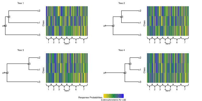
Figure S5.7: Simulation I: Four tree structures, ordered by increasing between-class correlation, in the synthetic data simulation. For each tree, the heatmap on the right display one of the 100 simulated sets of item response probabilities $\bm{\Theta}$. Beneath the heatmap are major food group indices of the $J=80$ items in the columns.

We considered LCMs with $K=3$ and $J=80$ items categorized into $G=7$ major food groups with $J_{1}=\cdots=J_{5}=10$ and $J_{6}=J_{7}=15$. Four distinct tree structures with $K=3$ leaves were considered corresponding to different levels of class separation (Figure S5.7). Trees 1 and 2 represent strong and moderate class separation. Trees 3 and 4 represent weak class separation. For each tree, we simulated 100 independent data sets for $N\in\{100,200,400\}$ individuals. See Supplementary Section S5.1 for additional setup details.

Figure 2 shows model performance comparison results. In the top row of Figure 2, compared to models (v) and (vi), DDT-LCM produces similar or significantly better recovery of the true tree topology and branch lengths. As classes become less separated from Tree 1 to Tree 4, all the methods produce higher errors in recovering the true tree, but DDT-LCM is far more accurate and stable than the rest. This is expected because (v) and (vi) perform LCM estimation and post hoc hierarchical clustering in two separate steps, which may not fully propagate the uncertainty into tree estimation. DDT-LCM fully accounts for uncertainty by performing joint estimation of the tree and other model parameters.

DDT-LCM also outperforms all the alternative methods, and is comparable to model (ii) true tree case, in recovering the LCM parameters by showing lower RMSEs of the estimated item response probabilities (middle row, Figure 2) and higher ARIs of individual class memberships (bottom row, Figure 2). This indicates that learning similarity information between classes guided by a jointly estimated tree may improve parameter estimates. If the true tree structure is known, additional estimation accuracy can be obtained. On the other hand, if the tree is misspecified at a structure far from the truth, the estimation accuracy may be much worse than DDT-LCM that estimates the tree and no better than the plain BayesLCM, which is particularly problematic under smaller sample sizes (e.g., $N=100$). DDT-LCM becomes more advantageous to other methods for weaker separation between the classes (from Tree 1 to 4). Larger sample sizes tend to make up for the performance disadvantage of other methods ($N=100$ to $400$). In particular, in Tree 1 where classes are well-separated, DDT-LCM performs similarly to the competing methods in all metrics. In this case, BayesLCM may be more computationally efficient and practically applicable because it does not involve sampling for the trees in the posterior sampling algorithm. As the classes become less separated, DDT-LCM takes advantage of between-class similarities and leads to accuracy gain. When sample sizes are small, information from tree-guided between-class similarities dominates the posterior distribution of the parameters. This dominance diminishes when data provides sufficient information under large samples size ($N=400$) in this small-scale fully synthetic study.

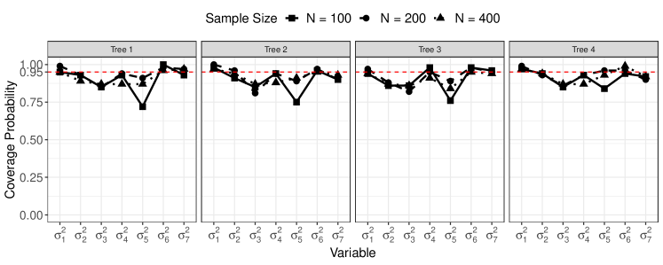
(a) Empirical coverage probabilities of the approximate 95% credible intervals The horizontal dashed lines indicate 95%.

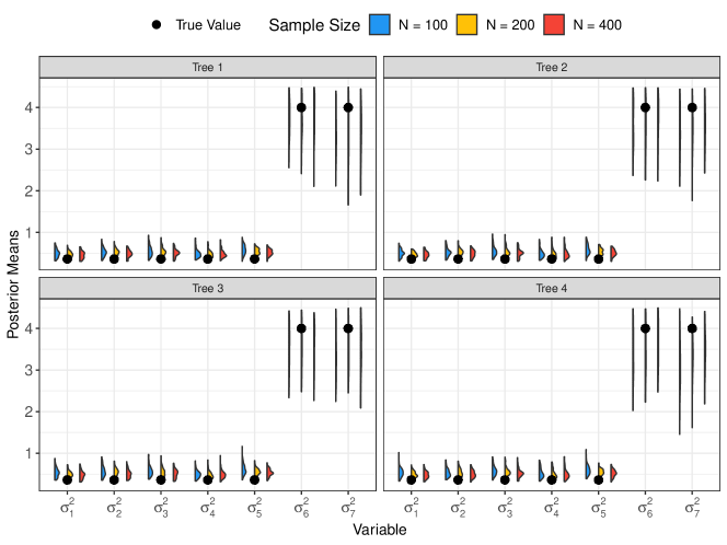
(b) Distribution of posterior mean estimates of $\bm{\sigma}^{2}$. For each $\sigma_{g}^{2}$, the three distributions correspond to sample sizes $N=100,200$, and 400 from left to right.

Figure S5.8: Simulation I: results of estimating group-specific diffusion variance parameter $\bm{\sigma}^{2}$, based on DDT-LCM from 100 datasets under different tree and sample size scenarios.

The better estimation performances of model (i) than model (iv) and (v) than (vi) of the LCM parameters implies that the different degrees of class separation in major food groups cannot be ignored. In addition, the empirical coverage probabilities of the 95% credible intervals of $\bm{\sigma}^{2}$ are close to the nominal level for larger sample sizes (Supplementary Figure S5.8(a)). The posterior mean estimates of the last two groups $\sigma_{6}^{2}$ and $\sigma_{7}^{2}$ have higher levels of uncertainty than the first five groups (Supplementary Figure S5.8 (b)), because the response probabilities of items in the last two groups are closer to the boundaries 0 or 1, making estimation more challenging. Simulation I demonstrates that by leveraging similarity information shared between latent classes and accounting for varying levels of class separation by major food groups, DDT-LCM achieves improved accuracy relative to common alternatives in estimating the tree structure, item response probabilities, and individual class assignments.

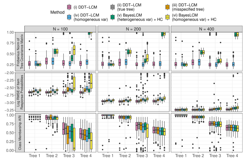
Figure 2: Simulation I: fully-synthetic data to compare parameter recovery performance for different trees and sample sizes for top) tree structure, middle) class profiles, and bottom) class memberships. Middle/Bottom): left to right: (i) – (vi). Top): (ii) and (iii) are omitted. Single linkage was used in (v) and (vi); results are similar for other linkage functions.

4.2 Simulation II: Semi-Synthetic Data

Simulation II mimicked the real data in the HCHS/SOL study to investigate whether DDT-LCM can confer statistical benefits under the realistic sample size and degree of between-class separation observed in the data. We also sought to evaluate a method to perform data-driven selection of $K$ in such scenarios. To this end, we simulated $J=78$ granular items categorized into $G=7$ major food groups, and $N=400,800$ subjects in $K=6$ latent classes. See Supplementary Section S5.2 for the detailed setup.

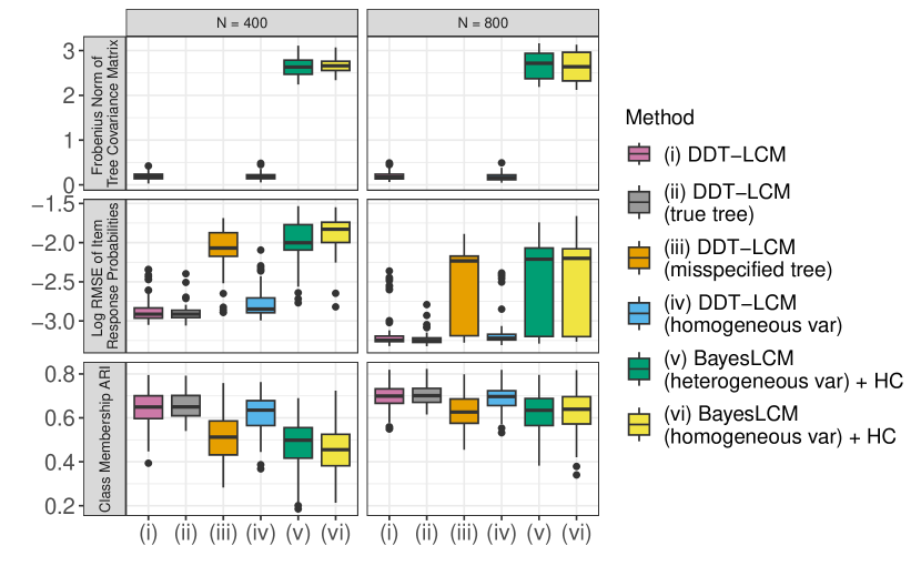
Figure 3: Simulation II to assess parameter recovery performance under weak separation and different sample sizes that mimic the real data: top) tree structure, middle) response probabilities, and bottom) class memberships. For methods (v) and (vi), single linkage is used; results are similar for other linkage functions.

Figure 3 displays the estimation results of DDT-LCM compared to alternative methods. Under the realistic weak class separation scenario, DDT-LCM is capable of more accurately recovering the true tree and LCM parameters under sample sizes below and above our real data size ($N=496$), suggesting its practical usefulness in deriving patterns for small-sized subpopulations. Moreover, we notice that for the majority of the simulated datasets, BayesLCM (with either heterogeneous or homogeneous variance) tends to merge two or more latent classes by forcing the class probabilities of these classes to near zero. The independent priors on $\bm{\Theta}$ do not facilitate BayesLCM to leverage similarity information across classes, leading to incorrect merging of classes. These results demonstrate the ability of DDT-LCM to handle complicated weakly separated real data scenarios by producing reliable estimates. Supplementary Figure S5.10 indicates that the proposed model (i) produces higher predictive log-likelihoods than model (iv). Supplementary Section S5.2 includes a discussion about diffusion variance parameter estimation.

The performance of DDT-LCM in the simulations has been demonstrated under a known $K$. To provide a practical estimation pipeline applicable to real-world data, Supplementary Section S5.2 describes a method to select $K$ in a data-driven manner.

5 Model Application to Dietary Intake Data

5.1 Data and Method

The Hispanic Community Health Study/Study of Latinos (HCHS/SOL) is a multi-center, community based cohort study of Hispanic/Latino adults in the United States (LaVange et al., 2010). A total of 16,415 participants aged between 18 and 74 years were recruited from field centers in Bronx, Chicago, Miami, and San Diego. In this analysis, we focus on dietary habits of $N=496$ participants with South American ethnic background. We selected this subgroup for its smaller sample size compared to other ethnic backgrounds and its known within-subgroup diet heterogeneity. Dietary intake was obtained from study participants via two 24-hour dietary recalls collected at baseline (2007-2011). These recalls were conducted using the Nutrition Data System for Research (NDSR) software developed by the Nutrition Coordinating Center at the University of Minnesota. Foods recorded from the dietary recalls were summarized into 50 broad food groups created from 165 NDSR food codes. Intake was quantified by servings per day. Participants with at least one reliable recall, defined by HCHS/SOL staff, were included for analysis. Participants with more than one reliable recall were averaged over the two days recorded. Existing literature has suggested that similarity may exist in dietary patterns among subgroups that share cultural ethnicity (Mattei et al., 2016; Stephenson et al., 2020b; Maldonado et al., 2021).

Our analysis considers dichotomized participant responses in the dietary recalls, where $Y_{ij}=1$ or 0 denotes presence or absence of exposure to food item $j$, defined by the commonality of serving frequency of that item. Highly consumed foods were defined as at least 3 servings a day ($Y_{ij}=1$) and 0 otherwise. Daily consumed foods were defined as at least one serving a day ($Y_{ij}=1$) and 0 otherwise. All other foods were defined as any consumption ($Y_{ij}=1$) and 0 otherwise. Items with less than 2.5% or more than 97.5% positive exposure were excluded to prevent inclusion of extreme intake data. Responses to $J=78$ the remaining food items were curated in total, belonging to $G=7$ nutrition groups: fat, fruit, grain, meat, dairy, sugar, and vegetables. A detailed list of food items and their major food groups included for analysis is provided in Supplementary Table LABEL:tab:item_labels. We apply the proposed DDT-LCM to our HCHS/SOL participant subset to estimate the exposure probabilities of food items corresponding to different dietary patterns. The candidate values for $K$ include $\{3,4,5,6,7,8\}$ and we would choose the $K$ that produced the largest average predictive log likelihood via five-fold cross-validation. For the optimal $K$, we ran the Gibbs sampler for 12,000 iterations and discarded the first 7,000 samples as burn-ins.

5.2 Results

Based on our model selection criteria, we selected a model with $K=6$ classes. We observed good convergence and mixing of our sampling algorithm. Figure 4 displays the derived dietary patterns and MAP tree under the selected model. The estimated diffusion variances for the 7 major food groups are 3.64 (fat), 1.75 (fruit), 2.88 (grain), 3.67 (meat), 3.58 (dairy), 2.60 (sugar), and 3.62 (vegetable). These estimates are consistent with the dietary pattern shown in Figure 4. The smallest variance occurs amongst fruit items. The probabilities of exposure to these fruit items do not vary much across latent classes, but the largest source of variation is identified in class 2. Fat, meat, dairy, and vegetable groups display the largest degrees of variability, implying that the dietary patterns exhibit major differences in items belonging to these major food groups. We assessed whether group-specific variance parameters were necessary as opposed to homogeneous variance parameters by the predictive likelihoods of DDT-LCM and “DDT-LCM (homogeneous var)” in five-fold cross-validation. The average log-likelihoods were $-3738.771$ and $-3746.070$, respectively. This indicated that DDT-LCM with group-specific variance parameters produced better predictive performance. These results emphasize the importance of group-specific variability parameters.

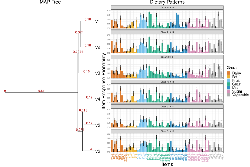
Figure 4: HCHS/SOL result with $K=6$ latent classes using binary responses from $N=496$ US adults with South American ethnicity. Left: the MAP tree structure over the latent classes. Numbers indicate the corresponding branch lengths. Right: dietary profiles for the $J=78$ food items belonging to $G=7$ different pre-defined nutrition groups, distinguished by different colors. The description of individual items is provided in Table LABEL:tab:item_labels with matching item labels on the x-axis. The numbers after the class labels in the facets indicate class prevalences. Error bars show the 95% credible intervals from the posterior distribution.

Classes 1 and 2 shared slightly similar behaviors in fruit, sugar, and vegetable food groups, and have a cophenetic distance of 0.834 on the MAP tree. Class 1 had higher probabilities of exposure to refined grain dry mixes, lean poultry, fried chicken, unsweetened coffee substitutes, white and fried potatoes, and other vegetables. Class 2 had higher probabilities of exposure to reduced fat salad dressing, cereal and bread with some whole grain, and whole grain snacks, lamb, milk and flavored milk, and all vegetables except for pickled foods. Class 3 shared some of these similarities with class 1 and class 2 (with a cophenetic distance of 0.815), but differed significantly in patterns within fat and meat groups with much lower exposure probabilities. Higher probabilities of exposure of this class were found in fruit-based snack, fried shellfish, sweetened fat free yogurt, unsweetened coffee substitutes, white potatoes and fried vegetables. Class 4 shared slightly similar dietary behaviors in all food groups with class 5 (with a cophenetic distance of 0.877) and had higher probabilities of exposure to a number of items, including salad dressing, citrus fruit, avocado and similar, dry grain mixes, crackers, lamb, lean poultry, whole milk, yogurt, sweetened fruit drinks, dessert, and dark-green vegetables. Class 5 had much higher probabilities of exposure to reduced-fat flavored milk, unsweetened coffee substitutes, and white potatoes. Class 6 shared common group-level attributes with class 4 (grains, meat, dairy, sugar) and class 5 (fruit, vegetables), at a cophenetic distance of 0.861. In the dairy group where classes 4 and 6 shared similarities, class 6 exhibited slightly higher probability of exposure to flavored milk.

We also compared these results with the standard Bayesian LCM, fit under $K=3,4,5,6,7$ classes, respectively. With the exception of the 3-class model, Bayesian LCMs (with either homogeneous or heterogeneous variances) did not converge and nearly zero class probabilities were estimated in at least one latent class. The item probability estimates in the sparse classes were all close to 0.5 with 95% credible intervals covering the complete probability range between 0 and 1. Although we might discard the sparse classes after implementing BayesLCM, the number of non-sparse classes was not consistently produced by the model under different $K$ values. This phenomenon echoes findings in prior literature (Lubke and Muthén, 2007; Park and Yu, 2018; Weller et al., 2020) that when latent classes are not sufficiently separated, convergence failure likely occurs due to small sample sizes.

6 Discussion

We derived dietary patterns of a small-sized subset of adult HCHS/SOL participants with South American ethnic background. Existing methods were challenged by weakly separated dietary patterns producing inaccurate inference of dietary patterns, especially in small-sized subpopulations with limited data. In addition, dietary patterns may show varying degrees of separation by major food groups because food consumption behaviors are often more similar for some food groups compared to others. We enhanced the inference of dietary patterns by introducing a tree-regularized Bayesian LCM that infers a hierarchical relationship among dietary patterns to facilitate sharing of statistical strength to make better estimates using limited data. Simulation and data analysis demonstrated that our method improved estimation of dietary patterns and individual class assignments relative to existing techniques based on classical Bayesian LCMs.

It is worth noting that DDT-LCM is perfectly suitable under larger sample sizes and produces comparable performances as classical LCMs at additional computational expense. In practice, because the boundary between large and small sample sizes is often unclear and must be determined relative to the actual degree of separation between dietary patterns in the data, DDT-LCM can guard against potential numerical and statistical instability.

DDT-LCM derives dietary patterns as an exploratory analysis to understand dietary behaviors among a subgroup that is typically undersized compared to the rest of the HCHS/SOL cohort. This analysis demonstrates how diet patterns of other small-sized subpopulations defined in HCHS/SOL can be derived, such as those formed by study-site and ethnic background that were excluded from Stephenson et al. (2020b) and De Vito et al. (2022) analysis (e.g. San Diego participants of Central American background or Bronx participants of Cuban background). We did not consider borrowing information from similar subpopulations or stratifying further by study site, which was the primary goal of RPC. DDT-LCM differs from RPC in application contexts. RPC identifies global and local differences in diet patterns across multiple pre-specified subpopulations. In contrast, DDT-LCM is designed for a single small-sized subpopulation to effectively learn the unique dietary patterns, while RPC is not suitable for weakly separated dietary patterns. If coupled with DDT-LCM in the local clustering process, RPC may become more sensitive at identifying the nuanced differences for each of the subpopulation at the local level.

The dietary recalls in the HCHS/SOL were collected only at baseline and thus our analysis was cross-sectional. Other studies have considered longitudinal designs to collect diet data (Nouri et al., 2021; Aljahdali et al., 2022). These longitudinal studies not only allow for studying cross-sectional diet-disease associations, but also the longitudinal associations. Extending DDT-LCM to longitudinal settings may better investigate how changes in diet are associated with changes in health outcomes, especially in small subpopulations.

Our study has a few limitations. First, we have not considered incorporating covariates of HCHS/SOL participants, such as age or sex, into modeling item response probabilities or class probabilities. Covariates may alleviate weak class separation by providing information about whether classes should be collapsed or not (Lubke and Muthén, 2007). Second, our model does not attempt to address recall biases associated with dietary intake. Previous validation studies have deemed the use of multiple dietary recalls as a reliable instrument for this cohort (Sorlie et al., 2010; Timon et al., 2016).

Further extensions may improve applicability and utility of the model. First, joint inference of $K$ and model parameters is a desirable alternative that may be useful in a broader set of applications (Miller and Harrison, 2018). Second, the major food groups included in our model amount to two-level item taxonomies. Additional insights into the subtle differences between the derived dietary patterns might be gained by incorporating multi-level taxonomies. Third, DDT-LCM assumes conditional independence between the item responses given a class, which can be relaxed to accommodate richer local dependence structures (e.g., Zhang, 2004). Finally, alternative posterior inference algorithms such as variational inference or message passing (Knowles et al., 2011) may further improve computational efficiency. We leave these topics for future research.

Supplementary Materials

Supplementary Materials contain supporting figures, tables, longer derivations, and additional results mentioned in Sections 2, 3, 4, and 5. The following sections are included:
S1: Generative Process of the Dirichlet Diffusion Tree
S3: Marginal Prior with Closed-Form Likelihood
S4: Posterior Sampling Algorithm
S5: Additional Simulation Study Details
S6: Food Items in the HCHS/SOL Dietary Recall

Code to reproduce simulations and data analysis is available online at github.com/xxx.

Supplement

Appendix S1 Generative Process of the Dirichlet Diffusion Tree

The DDT (Neal, 2003; Knowles and Ghahramani, 2015) is a generative model that consists of two components: 1) tree topologies ${\mathcal{T}}$ and divergence times $\bm{t}$, and 2) node parameters $\{\bm{\eta}_{u}\in\mathbb{R}^{J};u\in\mathcal{V}\}$ that follow Brownian motions along the branches when a tree topology and divergence times are given. In the following, we describe how the logit-transformed item response probabilities in DDT-LCM, or the leaf parameters of a random improper rooted binary tree, are generated from the DDT process.

In essence, the $K$ leaf parameters are the final destinations of $K$ different “particles” traveling from the origin $\bm{0}\in\mathbb{R}^{J}$ at time $t=0$ until $t=1$ according to Brownian motions in a self-reinforcing scheme. In a similar manner to the Chinese restaurant process (Aldous et al., 1985), the self-reinforcing scheme specifies a branching process where the more particles follow a particular path, the more likely subsequent particles will not diverge off this path. Specifically, the first particle simply travels without divergence according to a Brownian motion originating at the root parameter $\bm{\eta}_{u_{0}}=0$ at time $t=0$, and we obtain the first leaf parameter as the particle stops traveling at $t=1$ as well as the first tree branch. The second particle starts at the origin again and follows the path of the first particle until some divergence time $t$, after which it travels according to an independent Brownian motion and results in the second tree branch. The instantaneous probability of diverging on the infinitesimal interval $[t,t+dt)$ is $\frac{a(t)dt}{m}$, where $m$ is the number of particles that have previously traversed the current path (so $m=1$ for the second particle). Here, $a(t)$ is a divergence function satisfying $\int_{0}^{1}a(t)dt=\infty$ such that each particle leads to a new branch, hence a new leaf parameter, by $t=1$ almost surely. Similarly, each of the remaining particles follows an existing path initially. If a particle does not diverge before reaching a previous divergence point, it will follow one of the existing paths with probability proportional to the number of particles that previously travel along each path. After generating $K$ particles, we obtain the first set of components ${\mathcal{T}}$ and $\bm{t}$, as well as internal node parameters (divergence point parameters) and leaf parameters (unit time parameters). An graphical illustration of the above diffusion dynamics can be found in Figure 2(A) of Yao et al. (2023).

In the following, we describe two probabilistic distributions related to local characteristics of DDT that are used to construct the joint distribution of the DDT components in 1) and 2). First, if a particle is currently traveling along an existing path between $[t_{a},t_{b}]$ that has previously been visited by $m$ particles, the likelihood of the particle diverging at time $t>t_{a}$ is $P(\text{branch in }[t_{a},t])=1-\exp\{-[A(t)-A(t_{a})]/m\},$ where $A(t)=\int_{0}^{t}a(s)ds$ is called the cumulative branching function. For the choice of $a(t)=c/(1-t)$ in this paper, we have $A(t)=-c\log(1-t)$ and hence $P(\text{branch in }[t_{a},t])=1-\left(\frac{1-t}{1-t_{a}}\right)^{c/m}$. Therefore, compared to a smaller value of $c$, a larger $c$ places higher probability on large $t$, resulting in later divergence time. Second, inheriting from Brownian motions of the particles, the distribution of parameters associated with a non-root node $u$, conditional on the parameters associated with its parent node $pa(u)$, is a Gaussian distribution centered at $\bm{\eta}_{pa(u)}$ and variance proportional to the branch length $t_{u}-t_{pa(u)}$. This conditional distribution can be written as

$$\bm{\eta}_{u}\mid\bm{\eta}_{pa(u)},t_{u},t_{pa(u)}\sim\mathcal{N}\left(\bm{\eta}_{u};\bm{\eta}_{pa(u)},\sigma^{2}(t_{u}-t_{pa(u)})\right),$$

where $\sigma^{2}$ is used to scale the Brownian motions.

Appendix S2 The Tree-Structured Covariance Matrix

The tree-structured covariance matrix $\bm{\Sigma}$ not only has an important role of characterizing the DDT tree in this paper, but also sees important applications in phylogenetic tree literature (Revell et al., 2008; Yao et al., 2023). In fact, the tree-structured covariance matrix in our DDT context always has 1’s on the diagonal, and is strictly ultrametric and therefore nondegenerate almost surely (Martínez et al., 1994; Nabben and Varga, 1995). Any strictly ultrametric matrix has one-to-one correspondence to a rooted binary tree (Martínez et al., 1994), and this correspondence can be easily extended to an improper rooted binary tree (i.e., a DDT tree) by subtracting the length of the branch attached to the root node from all elements in $\bm{\Sigma}$. As a result, the distance between the associated matrices of two DDT trees is a reasonable metric for comparing the trees structures (Section 4).

Suppose we have items categorized into $G=2$ groups. The tree in Figure S2.5 is a possible structure over a 4-class LCM. The resulting tree-structured covariance matrix is

$$\bm{\Sigma}=\begin{pmatrix}1&0.5&0.22&0.22\\ 0.5&1&0.22&0.22\\ 0.22&0.22&1&0.7\\ 0.22&0.22&0.7&1\end{pmatrix}.$$

The diffusion variance of groups 1 and 2 are $\sigma_{1}^{2}=1.5^{2}$ and $\sigma_{2}^{2}=0.7^{2}$, respectively. Therefore, the row covariance of the two groups, as defined in equation (5), are $1.5^{2}\bm{\Sigma}$ and $0.7^{2}\bm{\Sigma}$, respectively. The cophenetic distance between $v_{1}$ and $v_{2}$ is 0.5, and that between $v_{1}$ and $v_{3}$ is 0.78.

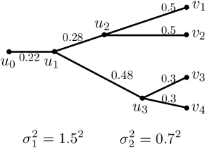
Figure S2.5: Example of a tree structure. For illustration purpose, we assume two groups of items are present with different diffusion variance parameters.

Appendix S3 Marginal Prior with Closed-Form Likelihood

We briefly describe the joint density $(\bm{\eta},{\mathcal{T}},\bm{t})$ based on equation (4). For an internal node $u\in\mathcal{V}^{I}$, let $l(u)$ and $r(u)$ be the number of leaf nodes under the left and right child of $u$, respectively, and let the total number of leaf nodes under node $u$ be $m(u)=l(u)+r(u)$. The structure of a tree (topology and branch lengths) generated under (4) can be viewed as a set of segments ${\mathcal{S}}({\mathcal{T}})=\left\{[uv]:0<t_{u}<t_{v}<1,u\in\mathcal{V}\setminus\mathcal{V}^{L}\right\}$. The joint probability density of node parameters and tree structure, conditional on the diffusion variance $\bm{\sigma}^{2}$ and the divergence function $a(t)=c/(1-t)$, is given by

$$P\left(\bm{\eta},{\mathcal{T}},\bm{t}\mid c,\bm{\sigma}^{2}\right)=\prod\limits_{[uv]\in{\mathcal{S}}({\mathcal{T}})}\underbrace{\frac{(l(v)-1)!(r(v)-1)!}{(m(v)-1)!}}_{\begin{subarray}{c}\text{tree topology }\\ P([uv])\end{subarray}}\underbrace{\vphantom{\frac{(l(v)-1)!(r(v)-1)!}{(m(v)-1)!}}c(1-t_{v})^{cJ_{v}-1}}_{\begin{subarray}{c}\text{branch lengths }\\ P(t_{v}\mid[uv],c)\end{subarray}}\underbrace{\vphantom{\frac{(l(v)-1)!(r(v)-1)!}{(m(v)-1)!}}\mathcal{N}_{J}(\bm{\eta}_{v}\mid\bm{\eta}_{u},(t_{v}-t_{u})\bm{D})}_{\begin{subarray}{c}\text{node parameters}\\ P(\bm{\eta}_{v}\mid[uv],\bm{\sigma}^{2},t_{v},t_{u})\end{subarray}},$$ (S3.1)

where $J_{v}=H_{m(v)-1}-H_{l(v)-1}-H_{r(v)-1}$ and $H_{n}=\sum\limits_{i=1}^{n}1/i$ is the $n$-th harmonic number. Here, $\bm{D}$ is a diagonal matrix whose $j$-th diagonal element equals $\sigma^{2}_{M_{j}}$, where $M_{j}$ is a major food group indicator such that $M_{j}=g$ if item $j$ belongs to group $g$. Refer to Knowles and Ghahramani (2015) for a detailed derivation of the joint density.

Appendix S4 Posterior Sampling Algorithm

We provide details of the three steps of the MH-within-Gibbs algorithm for posterior inference discussed in Section 3. Algorithm 1 gives a summary of the sampling steps.

S4.1 Metropolis-Hastings for Tree Topology and Divergence Times

As described in Section 3.1.2 of Yao et al. (2023), we first uniformly sample a non-root node $w\in\mathcal{V}$, and split the current tree ${\mathcal{T}}$ into two parts: a detached subtree ${\mathcal{T}}_{D}$ rooted at the parent of the sampled node $u=pa(w)$, and the remaining tree ${\mathcal{T}}_{R}$ after detaching ${\mathcal{T}}_{D}$ from the current tree. Next, we simulate a new node $u^{\prime}$ on ${\mathcal{T}}_{R}$ at time $t_{u^{\prime}}$ by following the branching process specified via divergence function $a(\cdot)$. A candidate tree ${\mathcal{T}}^{\prime}$ is formed by re-attaching the subtree ${\mathcal{T}}_{D}$ to the remaining tree at node $u^{\prime}$ and time $t_{u^{\prime}}$. The re-attaching time should be no later than the detaching time $t_{u}$ (i.e. $t_{u^{\prime}}<t_{u}$) to preserve branch lengths of ${\mathcal{T}}_{D}$, except for the branch connected to its root $u$. The corresponding proposal distribution from ${\mathcal{T}}$ to ${\mathcal{T}}^{\prime}$ is the probability of diverging at $u^{\prime}$ on the tree ${\mathcal{T}}_{R}$, and we denote the proposal distribution as $q(u^{\prime},{\mathcal{T}}_{R})$. The MH acceptance probability is then

$$\min\left\{1,\frac{p\left({\mathcal{T}}^{\prime},\bm{t}^{\prime}\mid\bm{\Omega}_{-({\mathcal{T}}^{\prime},\bm{t}^{\prime})}\right)q(u,{\mathcal{T}}_{R})}{p\left({\mathcal{T}},\bm{t}\mid\bm{\Omega}_{-({\mathcal{T}},\bm{t})}\right)q(u^{\prime},{\mathcal{T}}_{R})}\right\}.$$ (S4.1)

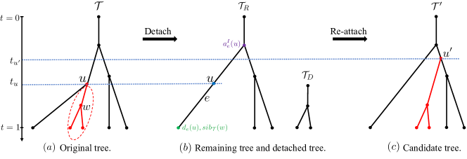
Figure S4.6: Example diagram of proposing a candidate tree ${\mathcal{T}}^{\prime}$ in the MH algorithm.

The target distribution is calculated as

$$\ p\left({\mathcal{T}},\bm{t}\mid\bm{\Omega}_{-({\mathcal{T}},\bm{t})}\right)\propto p({\mathcal{T}},\bm{t}\mid c)p\left(\bm{\eta}^{L}\mid{\mathcal{T}},\bm{t},\bm{\sigma}^{2}\right)$$

$$\propto \prod\limits_{[uv]\in{\mathcal{S}}({\mathcal{T}})}\frac{(l(v)-1)!(r(v)-1)!}{(m(v)-1)!}c(1-t_{v})^{cJ_{v}-1}\prod\limits_{g=1}^{G}\mathcal{M}\mathcal{N}_{K\times J_{g}}\left(\bm{\eta}^{L}_{g}\mid\bm{0},\sigma_{g}^{2}\bm{\Sigma}_{g},\bm{I}_{J_{g}}\right),$$ (S4.2)

which is similar to equation (S3.1) except that the last term here only involves the leaf parameters instead of all node parameters.

To calculate the ratio between the proposal distributions of the current tree and the candidate tree, we are only concerned about the branch $e$ of ${\mathcal{T}}_{R}$ from which the subtree ${\mathcal{T}}_{D}$ is detached, because ${\mathcal{T}}_{R}$ is shared by ${\mathcal{T}}$ and ${\mathcal{T}}^{\prime}$. With slight abuse of notation, denote $a_{e}^{I}(u)$ as the internal nodes on the path from root to the detached point $u$ on ${\mathcal{T}}_{R}$ earlier than $t_{u}$, and denote $d_{e}(u)$ as the nodes connected to $u$ on the branch $e$ of ${\mathcal{T}}_{R}$ after $t_{u}$. On the current tree ${\mathcal{T}}$, let the sibling node of $w$ be $sib(w)$, which is the child node of the detached point on ${\mathcal{T}}_{R}$. Then the proposal distribution of the current tree is

$$q(u,{\mathcal{T}}_{R})\propto\left[\prod\limits_{r\in a_{e}^{I}(u)}\exp\left\{[A(t_{pa(r)})-A(t_{r})]/m(r)\right\}\right]\left[\prod\limits_{r\in d_{e}(u)}\frac{m(r)}{m(pa(r))}\right]\frac{a(t_{u})}{m(sib(u))},$$ (S4.3)

where the $pa(r)$ is the parent node of $r$ on ${\mathcal{T}}_{R}$, and $m(r)$ counts the number of leaves possessed by the subtree of ${\mathcal{T}}_{R}$ rooted at $r$, or equivalently the number of “particles” passing through $r$ on ${\mathcal{T}}_{R}$. The first product term in equation (S4.3) is the probability that no divergence happens on the path from root to $u$ on ${\mathcal{T}}_{r}$, the second product term is the probability of selecting branches for particles to travel through in a self-reinforcing scheme, and the last term is the instantaneous probability of diverging at time $t_{u}$. The proposal distribution of the candidate tree is obtained by replacing ${\mathcal{T}}$ with ${\mathcal{T}}^{\prime}$ and $u$ with $u^{\prime}$.

S4.2 Augmented Gibbs Sampler for $\bm{\eta}^{L}$

For step (b), we sample the leaf parameter $\bm{\eta}^{L}$ by augmenting the conditional distribution $p\left(\bm{\eta}_{\cdot g}^{L}\mid\bm{\Omega}_{-\bm{\eta}},\bm{Y}\right)$ in equation (7) with two sets of auxiliary variables, applying the approach in Dalla Valle et al. (2021). The first auxiliary variables that follow logistic distributions ease the implementation of the Gibbs sampler, in a similar manner to the probit regression model (Albert and Chib, 1993). The second auxiliary variables that follow Pólya-Gamma distributions provide an elegant closed-form solution to dealing with the logistic link (Polson et al., 2013). We find empirically that incorporating both auxiliary variables significantly improves stability of the posterior chains, compared to the Pólya-Gamma technique alone.

For individual $i\in[N]$, item $j\in[J_{g}]$ in group $g\in[G]$, let

$$Y_{i,g,j}=I\{W_{i,g,j}>0\},\ \ W_{i,g,j}\mid Z_{i}=k\sim\mathrm{Logistic}\left(\eta_{g,j,k},1\right),$$ (S4.4)

where $\mathrm{Logistic}\left(\mu,s\right)$ stands for logistic distribution with location parameter $\mu$ and scale parameter $s$, whose probability density function is $f(x;\mu,s)=\frac{\exp\{(x-\mu)/s\}}{s\left(1+\exp\{(x-\mu)/s\}\right)^{2}}$, and cumulative distribution function is $H(x)=1/(1+\exp(-x))$ when $s=1$. We collect all elements $W_{i,g,j}$ into an $N\times J$ matrix $\bm{W}$. The augmented posterior distribution is

$$p\left(\bm{\eta}_{\cdot g}^{L},\bm{W}\mid\bm{\Omega}_{-\bm{\eta}},\bm{Y}\right) \propto p(\bm{\eta}_{\cdot g}^{L}\mid{\mathcal{T}},\bm{t},\bm{\sigma}^{2})p(\bm{Y}_{g}\mid\bm{W})P(\bm{W}\mid\bm{Z},\bm{\eta}_{\cdot g}^{L})$$

$$=\mathcal{M}\mathcal{N}_{K\times J_{g}}\left(\bm{0},\sigma_{g}^{2}\bm{\Sigma},\bm{I}_{J_{g}}\right)$$

$$\ \ \cdot\prod\limits_{i=1}^{N}\prod\limits_{j=1}^{J_{g}}\left[I\{W_{i,g,j}>0\}Y_{i,g,j}+I\{W_{i,g,j}\leq 0\}(1-Y_{i,g,j})\right]$$

$$\ \ \cdot\prod\limits_{i=1}^{N}\prod\limits_{k=1}^{K}\left\{\prod\limits_{j=1}^{J_{g}}\frac{\exp(w_{i,g,j}-\eta_{g,j,k})}{[1+\exp(w_{i,g,j}-\eta_{g,j,k})]^{2}}\right\}^{I\{Z_{i}=k\}}.$$ (S4.5)

We next deal with the logistic link by augmenting the distribution in equation (S4.5) with Pólya-Gamma auxiliary variables, as proposed in Polson et al. (2013). Specifically, we apply the following identity:

$$\frac{(e^{x})^{a}}{(1+e^{x})^{b}}=2^{-b}e^{\kappa x}\int_{0}^{\infty}\exp(-sx^{2}/2)p(s)ds,$$ (S4.6)

where $\kappa=a-b/2,a>0,b>0$, and $p(s)$ is the density function of a Pólya-Gamma (PG) distribution with shape parameter $b$ and exponential tilting parameter 0, denoted as PG$(b,0)$.

We apply the Pólya-Gamma identity in (S4.6) to the component in the curly bracket of the last line of (S4.5), which becomes

$$\prod\limits_{j=1}^{J_{g}}2^{-2}\int_{0}^{\infty}\exp\left[-s_{i,g,j}(w_{i,g,j}-\eta_{g,j,k})^{2}/2\right]p(s_{i,g,j})ds_{i,g,j},$$

where $s_{i,g,j}\sim\mathrm{PG}(2,0)$. Note that $\exp\left(-s_{i,g,j}\eta_{g,j,k}^{2}/2\right)p(s_{i,g,j})$ is the unnormalized density of a PG$(2,\eta_{g,j,k})$ random variable. Collecting all $s_{i,g,j}$ into an $N\times J$ matrix $\bm{S}$, we obtain the augmented posterior distribution with the two sets of auxiliary variables as

$$p\left(\bm{\eta}_{\cdot g}^{L},\bm{W},\bm{S}\mid\bm{\Omega}_{-\bm{\eta}},\bm{Y}\right) \propto p(\bm{\eta}_{\cdot g}^{L}\mid{\mathcal{T}},\bm{t},\bm{\sigma}^{2})p(\bm{Y}_{g}\mid\bm{W})P(\bm{W},\bm{S}\mid\bm{Z},\bm{\eta}_{\cdot g}^{L})$$

$$=\mathcal{M}\mathcal{N}_{K\times J_{g}}\left(\bm{\eta}_{\cdot g}^{L};\bm{0},\sigma_{g}^{2}\bm{\Sigma},\bm{I}_{J_{g}}\right)$$

$$\ \ \cdot\prod\limits_{i=1}^{N}\prod\limits_{j=1}^{J_{g}}\left[I\{W_{i,g,j}>0\}Y_{i,g,j}+I\{W_{i,g,j}\leq 0\}(1-Y_{i,g,j})\right]$$

$$\ \ \cdot\prod\limits_{i=1}^{N}\prod\limits_{k=1}^{K}\left\{\prod\limits_{j=1}^{J_{g}}2^{-2}\exp\left[-s_{i,g,j}(w_{i,g,j}-\eta_{g,j,k})^{2}/2\right]p(s_{i,g,j})\right\}^{I\{Z_{i}=k\}}.$$

The full conditional distributions are derived as follows.

The conditional distribution of $\bm{W}$: The random variables $\{W_{i,g,j}\}$ are mutually independent with conditional distributions

$$p\left(W_{i,g,j}\mid\bm{\eta},\bm{Z},\bm{S},\bm{Y}\right)$$

$$\propto \exp\left\{-\frac{1}{2s_{i,g,j}^{-1}\left(w_{i,g,j}-\eta_{Z_{i},g,j}\right)^{2}}\right\}\left[I\{w_{i,g,j}>0\}Y_{i,g,j}+I\{w_{i,g,j}\leq 0\}(1-Y_{i,g,j})\right],$$

which are truncated normal distributions. More precisely, the conditional distribution of $W_{i,g,j}$ is

$$P\left(W_{i,g,j}\mid\bm{\eta},\bm{Z},\bm{S},\bm{Y}\right)\sim\begin{cases}\mathcal{N}_{(0,\infty)}\left(\eta_{Z_{i},g,j},s_{i,g,j}^{-1}\right),&\text{ if }Y_{i,g,j}=1\\ \mathcal{N}_{(-\infty,0]}\left(\eta_{Z_{i},g,j},s_{i,g,j}^{-1}\right),&\text{ if }Y_{i,g,j}=0\end{cases},$$ (S4.7)

where $\mathcal{N}_{E}\left(\mu,\tau\right)$ indicates a normal distribution with mean $\mu$ and variance $\tau$ restricted to the interval $E$.

The conditional distribution of $\bm{S}$: The full conditional distributions of the Pólya-Gamma random variables $s_{i,g,j}$ are mutually independent and

$$P(s_{i,g,j}\mid\bm{\eta},\bm{Z},\bm{S},\bm{Y}) \propto\exp\left\{-s_{i,g,j}\left(w_{i,g,j}-\eta_{Z_{i},g,j}\right)^{2}/2\right\}p(s_{i,g,j})$$

$$\sim\mathrm{PG}\left(2,w_{i,g,j}-\eta_{Z_{i},g,j}\right).$$ (S4.8)

The conditional distribution of $\bm{\eta}^{L}$: The leaf parameters $\bm{\eta}_{\cdot g}^{L}$ of each item group $g$ are mutually independent. Let $\mathrm{vec}\left(\bm{\eta}_{\cdot g}^{L}\right)$ denote the $KJ_{g}\times 1$-vector created from stacking columns of $\bm{\eta}_{\cdot g}^{L}$, and let $\otimes$ denote the Kronecker product. The full conditional distribution of $\mathrm{vec}\left(\bm{\eta}_{\cdot g}^{L}\right)$ is

$$P(\mathrm{vec}\left(\bm{\eta}_{\cdot g}^{L}\right)\mid\bm{W},\bm{S},\bm{\Omega}_{-\bm{\eta}},\bm{Y})$$

$$\propto\exp\left\{-\frac{1}{2}\mathrm{vec}\left(\bm{\eta}_{\cdot g}^{L}\right)^{\top}\left(\sigma_{g}^{2}\bm{\Sigma}_{g}\otimes\bm{I}_{J_{g}}\right)^{-1}\mathrm{vec}\left(\bm{\eta}_{\cdot g}^{L}\right)\right\}\prod\limits_{i=1}^{N}\prod\limits_{k=1}^{K}\left\{\prod\limits_{j=1}^{J_{g}}\exp\left[-(w_{i,g,j}-\eta_{g,j,k})^{2}/2\right]\right\}^{I\{Z_{i}=k\}}$$

$$=\exp\left\{-\frac{1}{2}\mathrm{vec}\left(\bm{\eta}_{\cdot g}^{L}\right)^{\top}\left(\bm{\Gamma}_{g}+\sigma_{g}^{-2}\bm{\Sigma}_{g}^{-1}\otimes\bm{I}_{J_{g}}\right)\mathrm{vec}\left(\bm{\eta}_{\cdot g}^{L}\right)+\mathrm{vec}\left(\bm{\eta}_{\cdot g}^{L}\right)\mathrm{vec}\left(\bm{\xi}_{g}\right)\right\},$$

where $\bm{\xi}_{g}$ denotes a $K\times J_{g}$ matrix whose $(k,j)$-th entry is $\sum\limits_{i=1}^{N}I\{Z_{i}=k\}u_{i,g,j}w_{i,g,j}$, and $\bm{\Gamma}_{g}=\mathrm{diag}\left(\mathrm{vec}\left(\bm{\gamma}_{g}\right)\right)$ with $\bm{\gamma}_{g}$ being a $K\times J_{g}$ matrix whose $(k,j)$-th entry is $\sum\limits_{i=1}^{N}I\{Z_{i}=k\}u_{i,g,j}$. Therefore, the conditional distribution of $\bm{\eta}_{\cdot g}^{L}$ is

$$P(\bm{\eta}_{\cdot g}^{L}\mid\bm{W},\bm{U},\bm{\Omega}_{-\bm{\eta}},\bm{Y})\sim\mathcal{N}_{KJ_{g}}\left(\bm{\mu}_{g},\bm{\Psi}_{g}\right),$$ (S4.9)

where

$$\bm{\Psi}_{g}=\left(\bm{D}_{g}+\sigma_{g}^{-2}\bm{\Sigma}_{g}^{-1}\otimes\bm{I}_{J_{g}}\right)^{-1},\ \ \bm{\mu}_{g}=\bm{\Psi}_{g}\mathrm{vec}\left(\bm{\xi}_{g}^{(1)}\right).$$

S4.3 Gibbs Sampler for the Remaining Parameters

Apart from the model parameters discussed in the previous sections, we derive the divergence hyperparameter $c$ and diffusion variance $\bm{\sigma}^{2}$ of the DDT process, as well as the latent class indicators $\bm{Z}$ and class prevalence $\bm{\pi}$ in this section. Utilizing equation (S3.1), the full conditional distribution of the divergence hyperparameter $c$ is

$$p(c\mid\bm{\Omega}_{-c}) \propto p({\mathcal{T}},\bm{t}\mid c)\ p(c)\ \propto\prod\limits_{[uv]\in{\mathcal{S}}({\mathcal{T}})}c(1-t_{v})^{cJ_{v}-1}c^{\alpha_{c}-1}e^{-c\beta_{c}}$$

$$=c^{K-1+\alpha_{c}-1}\exp\left\{-c\left(\beta_{c}-\sum_{u\in\mathcal{V}^{I}}J_{u}\log(1-t_{u})\right)\right\}$$

$$\sim G\left(K-1+\alpha_{c},\beta_{c}-\sum_{u\in\mathcal{V}^{I}}J_{u}\log(1-t_{u})\right).$$ (S4.10)

The full conditional distributions of $\bm{\sigma}_{g}^{2}$ of each item group $g$ are mutually independent with

$$p(\sigma_{g}^{2}\mid\bm{\Omega}_{-c}) \propto p(\bm{\eta}_{\cdot g}^{L}\mid{\mathcal{T}},\bm{t},\sigma_{g}^{2})p(\sigma_{g}^{2})$$

$$\propto\left(\sigma_{g}^{2}\right)^{-J_{g}K/2}\exp\left\{-\frac{1}{2}\sigma_{g}^{-2}\mathrm{Tr}\left((\bm{\eta}_{\cdot g}^{L})^{\top}\bm{\Sigma}_{g}^{-1}(\bm{\eta}_{\cdot g}^{L})\right)\right\}\left(\sigma_{g}^{2}\right)^{-\alpha_{\sigma_{g}}-1}\exp\left(-\beta_{\sigma_{g}}/\sigma_{g}^{2}\right)$$

$$=\left(\sigma_{g}^{2}\right)^{-J_{g}K/2-\alpha_{\sigma_{g}}-1}\exp\left(-(\beta_{\sigma_{g}}+S_{g}/2)\sigma_{g}^{-2}\right)$$

$$\sim IG\left(J_{g}K/2+\alpha_{\sigma_{g}},\beta_{\sigma_{g}}+S_{g}/2\right),$$ (S4.11)

where $S_{g}=\mathrm{Tr}\left((\bm{\eta}_{\cdot g}^{L})^{\top}\bm{\Sigma}_{g}^{-1}(\bm{\eta}_{\cdot g}^{L})\right)$ and $\mathrm{Tr}(\bm{X})$ denotes the trace of a square matrix $\bm{X}$.

The full conditional distribution of $\bm{Z}_{i}$ can be obtained from

$$p(Z_{i}=k\mid\bm{\Omega}_{-\bm{Z}},\bm{Y}) \propto\pi_{k}\prod\limits_{g=1}^{G}\prod\limits_{j=1}^{J_{g}}(\theta_{g,j,k})^{Y_{i,g,j}}(1-\theta_{g,j,k})^{1-Y_{i,g,j}},$$

which is a categorical distribution on $[K]$ with the probability of taking value $k$ being

$$\frac{\pi_{k}\prod\limits_{g=1}^{G}\prod\limits_{j=1}^{J_{g}}(\theta_{g,j,k})^{Y_{i,g,j}}(1-\theta_{g,j,k})^{1-Y_{i,g,j}}}{\sum\limits_{m=1}^{K}\pi_{m}\prod\limits_{g=1}^{G}\prod\limits_{j=1}^{J_{g}}(\theta_{m,g,j})^{Y_{i,g,j}}(1-\theta_{m,g,j})^{1-Y_{i,g,j}}}.$$ (S4.12)

Appendix S5 Additional Simulation Study Details

The same hyperparameter setting in the priors of $\sigma_{g}^{2}$, $c$, and $\bm{\pi}$ applies to the synthetic (Section 4.1) and semi-synthetic (Section 4.2) data simulations and real data application (Section 5). Specifically, the priors for all $\sigma_{g}^{2}$ are specified as Inverse-Gamma$(2,2)$, the prior for $c$ is Gamma$(1,1)$ and the prior for $\bm{\pi}$ is Dirichlet$(5,\ldots,5)$. For all simulation scenarios, we run the sampling algorithm for 8,000 iterations and discard the first 5,000 burn-in samples for each simulated dataset. Label switching is addressed post hoc via the Equivalence Classes Representative (ECR, Papastamoulis, 2014).

S5.1 Simulation I: Synthetic Data Setup and Results

The class prevalence is set to $\bm{\pi}=(0.4,0.3,0.3)$, and the group-specific diffusion variances are $\sigma_{g}^{2}=0.6^{2}$ for $g\leq 5$ and $\sigma_{g}^{2}=2^{2}$ for $g=6,7$. For each tree, we simulate 20 sets of response probabilities, for each of which we simulate 5 independent datasets of multivariate binary responses for $N\in\{100,200,400\}$ individuals following LCMs; hence, a total of 100 independent datasets for each $N$. For the “DDT-LCM (misspecified tree)” method, the misspecified tree is fixed at the structure Tree 4 when we perform posterior sampling of the Tree 1 and Tree 2 scenarios, and the misspecified tree for Tree 3 and Tree 4 scenarios is fixed at the structure of Tree 1.

S5.2 Simulation II: Semi-Synthetic Data Simulation Setup

We set the true tree as the MAP tree (left of Figure 4) estimated by DDT-LCM from the HCHS/SOL data. The MAP tree implies weakly separated classes with between-class correlations at least 0.8. We set the class prevalence to be the posterior mean estimated from the HCHS/SOL data analysis, which is $\bm{\pi}=(0.14,0.14,0.2,0.18,0.17,0.16)$. The group-specific diffusion variances are $\sigma_{g}^{2}=1^{2}$ for $g\leq 5$ and $\sigma_{g}^{2}=2.3^{2}$ for $g=6,7$. Based on the MAP tree (Figure 4), we simulate 20 sets of response probabilities, for each of which we simulate 5 independent datasets of multivariate binary responses for $N\in\{400,800\}$ individuals following LCMs; hence, a total of 100 independent datasets for each $N$. Figure S5.10 displays the misspecified tree structured used in method “DDT-LCM (misspecified tree)”.

Figure S5.9: Simulation II: Misspecified tree structure for method “DDT-LCM (misspecific tree)”.

Figure S5.10: Simulation II: log-likelihood comparison to choose group-specific or homogeneous diffusion variance parameters. The red dashed line indicates 0.

Data-driven choice of $K$

The performance of DDT-LCM in Simulations I and II has been demonstrated under a known number of latent classes $K$. To provide a practical estimation pipeline applicable to real-world data, we next briefly describe a method to select $K$ in a data-driven manner. In particular, we focus on the semi-synthetic data because it represents a scenario close to our real data application, while our selection method can be generalized to any situations.

Our rationale here is to apply a practically useful criterion that leans towards a model with good out-of-sample predictive performance while remaining parsimonious. Viewing $K$ as a hyperparameter, we choose the $K$ that yields the average largest predictive log-likelihood on validation datasets from 5-fold cross-validation. Specifically, the observations of $N$ individuals are randomly split into a training set and a testing set according to a 4:1 ratio. For the $s$-th training set, $s\in[5]$, we apply the Gibbs sampler and obtain the posterior means of the class prevalences $\widehat{\pi}$ and response probabilities $\widehat{\theta}$. The predictive likelihood on the corresponding testing set is computed as

$$p_{K,s}^{test}=\prod\limits_{i\in I^{test}_{s}}\left[\sum\limits_{k=1}^{K}\widehat{\pi}_{k}\prod\limits_{g=1}^{G}\prod\limits_{j=1}^{J_{g}}\left(\widehat{\theta}_{g,j,k}\right)^{Y_{i,g,j}}\left(1-\widehat{\theta}_{g,j,k}\right)^{1-Y_{i,g,j}}\right],$$

where $I^{test}_{s}$ denotes the indices of individuals belonging to the $s$-th testing set. The average predictive log-likelihood is then calculated as $l_{K}^{test}=\frac{1}{5}\sum\limits_{s=1}^{5}\log p_{K,s}^{test}$. The model with a larger $l_{K}^{test}$ is preferred.

We conduct a simulation study to evaluate the performance of $l_{K}^{test}$ on the selection of $K$, focusing on semi-synthetic scenario with the truth $K_{\mathrm{true}}=6$. For each candidate number of classes $K_{\mathrm{candidate}}$ from $\{4,5,6,7,8\}$, we compute the above measure $l_{K_{\mathrm{candidate}}}^{test}$. We find that for $N=400$, the percentages of datasets that each of $K=4,5,6,7,8$ is selected are 11%, 36%, 45% (truth), 7%, and 1%, respectively; for $N=800$, the percentages are 2%, 15%, 73% (truth), 8%, and 2%, respectively. This result indicates that the predictive log-likelihood is a reasonable metric to select the best $K$, and the selection accuracy increases with sample size. While we acknowledge that selecting the correct $K$ is not an easy task under the relatively small sample size $N=496$ in our real data application, the practical utility of our procedure is still valuable in analysis of real-world datasets. Developing a rigorous understanding of the theoretical behavior of this measure requires further investigation.

We choose the $K$ that yields the average largest predictive log-likelihood on validation datasets from 5-fold cross-validation. Specifically, the observations of $N$ individuals are randomly split into a training set and a testing set according to a 4:1 ratio. For the $s$-th training set, $s\in[5]$, we apply the Gibbs sampler and obtain the posterior means of the class prevalences $\widehat{\pi}$ and response probabilities $\widehat{\theta}$. The predictive likelihood on the corresponding testing set is computed as

$$p_{K,s}^{test}=\prod\limits_{i\in I^{test}_{s}}\left[\sum\limits_{k=1}^{K}\widehat{\pi}_{k}\prod\limits_{g=1}^{G}\prod\limits_{j=1}^{J_{g}}\left(\widehat{\theta}_{g,j,k}\right)^{Y_{i,g,j}}\left(1-\widehat{\theta}_{g,j,k}\right)^{1-Y_{i,g,j}}\right],$$

where $I^{test}_{s}$ denotes the indices of individuals belonging to the $s$-th testing set. The average predictive log-likelihood is then calculated as $l_{K}^{test}=\frac{1}{5}\sum\limits_{s=1}^{5}\log p_{K,s}^{test}$. The model with a larger $l_{K}^{test}$ is preferred.

Gelman et al. (2014) provides a comprehensive overview of commonly applied predictive information criteria for evaluating Bayesian models. We tried the Deviance Information Criterion (DIC, Spiegelhalter et al. (2002)) and Widely Applicable Information Criterion (WAIC, Watanabe (2010)) and computed these two measures in two alternative ways detailed in Gelman et al. (2014). However, our preliminary simulation results imply that neither DIC nor WAIC work well for the selection of $K$ in DDT-LCM. In particular, DIC it always over-estimates the suitable $K$ while WAIC also sometimes favors a large $K$. This inconsistency behavior of DIC has also been observed in previous literature studying finite mixture models Gelman et al. (2014); Spiegelhalter et al. (2014); Gu et al. (2021); Watanabe (2021). On the other hand, while Watanabe (2010) has justified that WAIC is asymptotically equivalent to Bayesian leave-one-out cross-validation, our simulation scenarios, have relatively small sample sizes, which challenges the asymptotic consistency property.

Choice of diffusion variance

We provide a practical procedure to select group-specific or diffusion variance specification when analyzing real data. For DDT-LCM and “DDT-LCM (homogeneous var)” methods under a pre-specified $K$, we choose the method that produces a higher average predictive log-likelihood from cross-validation. Figure S5.10 shows the comparison results of the two methods over 100 simulated semi-synthetic datasets. For both sample sizes $N=400$ and 800, DDT-LCM with group-specific diffusion variance parameters performs better than the one with homogeneous variance parameters.

Appendix S6 Food Items in the HCHS/SOL Dietary Recall

Table S6.1: Food items included in data application to HCHS/SOL 24-hour dietary recall data. Daily consumed foods: (High) at least one serving a day, and (Low) less than one serving a day. All other foods: (+) any consumption, and (-) no consumption. The last column indicates the percentages of individuals having positive exposure to the food items. Only foods with $\geq 5\%$ or $\leq 95\%$ level 1 exposure were included in the analysis.

Group	Item Label	Description	Level 0	Level 1	% Level 1
Dairy	diary_1	Milk - Whole	-	+	49.19
	diary_2	Milk - Low Fat and Fat Free	-	+	44.15
	diary_3	Ready-to-drink Flavored Milk - Reduced Fat	-	+	14.31
	diary_4	Ready-to-drink Flavored Milk - Low Fat and Fat Free	-	+	6.05
	diary_5	Sweetened Flavored Milk Beverage Powder with Non-fat Dry Milk	-	+	63.10
	diary_6	Artificially Sweetened Flavored Milk Beverage Powder with Non-fat Dry Milk	-	+	30.24
	diary_7	Yogurt - Sweetened Low Fat	-	+	6.05
	diary_8	Yogurt - Sweetened Fat Free	-	+	9.68
	diary_9	Yogurt - Nondairy	-	+	5.85
	diary_10	Dairy-based Artificially Sweetened Meal Replacement/Supplement	-	+	10.89
	diary_11	Infant Formula	-	+	33.67
Fat	fat_1	Cream - Reduced Fat	-	+	11.90
	fat_2	Margarine - Regular	-	+	13.10
	fat_3	Butter and Other Animal Fats - Reduced Fat	-	+	24.40
	fat_4	Salad Dressing - Regular	-	+	32.86
	fat_5	Salad Dressing - Reduced Fat/Reduced Calorie/Fat Free	-	+	6.05
	fat_6	Gravy - Regular	-	+	17.34
	fat_7	Gravy - Reduced Fat/Fat Free	-	+	12.70
Fruit	fruit_1	Citrus Juice	-	+	13.10
	fruit_2	Fruit Juice excluding Citrus Juice	-	+	57.46
	fruit_3	Citrus Fruit	-	+	29.64
	fruit_4	Fruit excluding Citrus Fruit	-	+	47.38
	fruit_5	Avocado and Similar	-	+	57.86
	fruit_6	Fried Fruits	-	+	41.94
	fruit_7	Fruit-based Savory Snack	-	+	47.38
Grain	grain_1	Grains, Flour and Dry Mixes - Whole Grain	-	+	11.49
	grain_2	Grains, Flour and Dry Mixes - Some Whole Grain	-	+	20.36
	grain_3	Grains, Flour and Dry Mixes - Refined Grain	Low	High	15.73
	grain_4	Loaf-type Bread and Plain Rolls - Refined Grain	-	+	12.50
	grain_5	Other Breads (quick breads, corn muffins, tortillas) - Some Whole Grain	-	+	63.91
	grain_6	Other Breads (quick breads, corn muffins, tortillas) - Refined Grain	-	+	20.56
	grain_7	Crackers - Whole Grain	-	+	8.47
	grain_8	Crackers - Some Whole Grain	-	+	30.04
	grain_9	Pasta - Whole Grain	-	+	5.44
	grain_10	Ready-to-eat Cereal (not presweetened) - Whole Grain	-	+	6.85
	grain_11	Ready-to-eat Cereal (presweetened) - Whole Grain	-	+	34.27
	grain_12	Ready-to-eat Cereal (presweetened) - Some Whole Grain	-	+	66.33
	grain_13	Cakes, Cookies, Pies, Pastries, Danish, Doughnuts and Cobblers - Some Whole Grain	-	+	46.17
	grain_14	Snack Bars - Whole Grain	-	+	10.89
	grain_15	Snack Chips - Whole Grain	-	+	33.67
	grain_16	Flavored Popcorn	-	+	15.32
Meat	meat_1	Lamb	-	+	44.76
	meat_2	Lean Lamb	-	+	15.12
	meat_3	Game	-	+	15.12
	meat_4	Poultry	-	+	33.06
	meat_5	Lean Poultry	Low	High	20.36
	meat_6	Fried Chicken - Commercial Entrée and Fast Food	-	+	14.72
	meat_7	Lean Fish - Fresh and Smoked	-	+	7.06
	meat_8	Fried Fish - Commercial Entrée and Fast Food	-	+	20.16
	meat_9	Fried Shellfish - Commercial Entrée and Fast Food	-	+	11.69
	meat_10	Lean Cold Cuts and Sausage	-	+	9.27
	meat_11	Nuts and Seeds	-	+	30.04
	meat_12	Nut and Seed Butters	-	+	23.19
Sugar	sugar_1	Sugar	Low	High	36.49
	sugar_2	Syrup, Honey, Jam, Jelly, Preserves	-	+	46.77
	sugar_3	Sauces, Sweet - Reduced Fat/Reduced Calorie/Fat Free	-	+	11.49
	sugar_4	Chocolate Candy	-	+	23.79
	sugar_5	Sweetened Soft Drinks	-	+	6.25
	sugar_6	Artificially Sweetened Soft Drinks	-	+	12.50
	sugar_7	Sweetened Fruit Drinks	-	+	50.20
	sugar_8	Artificially Sweetened Fruit Drinks	-	+	6.45
	sugar_9	Artificially Sweetened Tea	-	+	51.21
	sugar_10	Sweetened Coffee	-	+	7.46
	sugar_11	Unsweetened Coffee	-	+	9.27
	sugar_12	Sweetened Coffee Substitutes	-	+	36.69
	sugar_13	Unsweetened Coffee Substitutes	-	+	50.00
	sugar_14	Nondairy-based Unsweetened Meal Replacement/Supplement	-	+	13.71
	sugar_15	Miscellaneous Dessert	-	+	11.69
Vegetable	veg_1	Dark-green Vegetables	-	+	40.73
	veg_2	Deep-yellow Vegetables	-	+	14.11
	veg_3	Tomato	Low	High	12.50
	veg_4	White Potatoes	-	+	50.81
	veg_5	Fried Potatoes	-	+	12.10
	veg_6	Other Starchy Vegetables	-	+	9.48
	veg_7	Other Vegetables	Low	High	43.35
	veg_8	Fried Vegetables	-	+	44.15
	veg_9	Vegetable Juice	-	+	34.48
	veg_10	Pickled Foods	-	+	7.06

References

- (1)
- Albert and Chib (1993) Albert, J. H. and Chib, S. (1993), ‘Bayesian analysis of binary and polychotomous response data’, Journal of the American Statistical Association 88(422), 669–679.
- Aldous et al. (1985) Aldous, D. J., Ibragimov, I. A., Jacod, J. and Aldous, D. J. (1985), Exchangeability and related topics, Springer.
- Aljahdali et al. (2022) Aljahdali, A. A., Baylin, A., Ruiz-Narvaez, E. A., Kim, H. M., Cantoral, A., Tellez-Rojo, M. M. et al. (2022), ‘Sedentary patterns and cardiometabolic risk factors in Mexican children and adolescents: Analysis of longitudinal data’, International Journal of Behavioral Nutrition and Physical Activity 19(1), 143.
- Allman et al. (2009) Allman, E. S., Matias, C. and Rhodes, J. A. (2009), ‘Identifiability of parameters in latent structure models with many observed variables’, The Annals of Statistics pp. 3099–3132.
- Billera et al. (2001) Billera, L. J., Holmes, S. P. and Vogtmann, K. (2001), ‘Geometry of the space of phylogenetic trees’, Advances in Applied Mathematics 27(4), 733–767.
- Blei et al. (2003) Blei, D. M., Jordan, M. I., Griffiths, T. L. and Tenenbaum, J. B. (2003), Hierarchical topic models and the nested chinese restaurant process, in ‘Proceedings of the 16th International Conference on Neural Information Processing Systems’, NIPS’03, MIT Press, Cambridge, MA, USA, pp. 17–24.
- Blom et al. (2017) Blom, M. P. K., Bragg, J. G., Potter, S. and Moritz, C. (2017), ‘Accounting for uncertainty in gene tree estimation: Summary-coalescent species tree inference in a challenging radiation of Australian lizards’, Systematic Biology 66(3), 352–366.
- Dalla Valle et al. (2021) Dalla Valle, L., Leisen, F., Rossini, L. and Zhu, W. (2021), ‘A Pólya–Gamma Sampler for A Generalized Logistic Regression’, Journal of Statistical Computation and Simulation 91(14), 2899–2916.
- De Vito et al. (2022) De Vito, R., Stephenson, B., Sotres-Alvarez, D., Siega-Riz, A.-M., Mattei, J., Parpinel, M. et al. (2022), ‘Shared and ethnic background site-specific dietary patterns in the Hispanic Community Health Study/Study of Latinos (HCHS/SOL)’.
- Dietary Guidelines Advisory Committee (2020) Dietary Guidelines Advisory Committee (2020), Scientific report of the 2020 dietary guidelines advisory committee: Advisory report to the secretary of agriculture and secretary of health and human services, Technical report, U.S. Department of Agriculture, Agricultural Research Service.
- Engeset et al. (2015) Engeset, D., Hofoss, D., Nilsson, L. M., Olsen, A., Tjønneland, A. and Skeie, G. (2015), ‘Dietary patterns and whole grain cereals in the Scandinavian countries – differences and similarities. the HELGA project’, Public Health Nutrition 18(5), 905–915.
- Gelman et al. (2014) Gelman, A., Hwang, J. and Vehtari, A. (2014), ‘Understanding predictive information criteria for Bayesian models’, Statistics and Computing 24(6), 997–1016.
- Ghahramani et al. (2010) Ghahramani, Z., Jordan, M. and Adams, R. P. (2010), Tree-structured stick breaking for hierarchical data, in ‘Advances in Neural Information Processing Systems’, Vol. 23, Curran Associates, Inc.
- Goodman (1974) Goodman, L. A. (1974), ‘Exploratory latent structure analysis using both identifiable and unidentifiable models’, Biometrika 61(2), 215–231.
- Gu et al. (2021) Gu, Y., Erosheva, E. A., Xu, G. and Dunson, D. B. (2021), ‘Dimension-grouped mixed membership models for multivariate categorical data’, arXiv:2109.11705 . arXiv:2109.11705.
- Hubert and Arabie (1985) Hubert, L. and Arabie, P. (1985), ‘Comparing partitions’, Journal of Classification 2(1), 193–218.
- Kant (2004) Kant, A. K. (2004), ‘Dietary patterns and health outcomes’, Journal of the American Dietetic Association 104(4), 615–635.
- Knowles and Ghahramani (2015) Knowles, D. A. and Ghahramani, Z. (2015), ‘Pitman-Yor diffusion trees for Bayesian hierarchical clustering’, IEEE transactions on pattern analysis and machine intelligence 37(2), 271–289.
- Knowles et al. (2011) Knowles, D. A., Van Gael, J. and Ghahramani, Z. (2011), ‘Message passing algorithms for the Dirichlet diffusion tree’, Proceedings of the 28th International Conference on Machine Learning .
- LaVange et al. (2010) LaVange, L. M., Kalsbeek, W. D., Sorlie, P. D., Avilés-Santa, L. M., Kaplan, R. C., Barnhart, J. et al. (2010), ‘Sample design and cohort selection in the Hispanic Community Health Study/Study of Latinos’, Annals of Epidemiology 20(8), 642–649.
- Lazarsfeld (1950) Lazarsfeld, P. F. (1950), ‘The logical and mathematical foundation of latent structure analysis’, Studies in Social Psychology in World War II Vol. IV: Measurement and Prediction pp. 362–412.
- Li et al. (2023) Li, M., Park, D. E., Aziz, M., Liu, C. M., Price, L. B. and Wu, Z. (2023), ‘Integrating sample similarities into latent class analysis: A tree-structured shrinkage approach’, Biometrics 79(1), 264–279.
- Lubke and Muthén (2007) Lubke, G. and Muthén, B. O. (2007), ‘Performance of factor mixture models as a function of model size, covariate effects, and class-specific parameters’, Structural Equation Modeling: A Multidisciplinary Journal 14(1), 26–47.
- Maldonado et al. (2021) Maldonado, L. E., Adair, L. S., Sotres-Alvarez, D., Mattei, J., Mossavar-Rahmani, Y., Perreira, K. M. et al. (2021), ‘Dietary patterns and years living in the United States by Hispanic/Latino heritage in the Hispanic Community Health Study/Study of Latinos (HCHS/SOL)’, The Journal of Nutrition 151(9), 2749–2759.
- Martínez et al. (1994) Martínez, S., Michon, G. and Martín, J. S. (1994), ‘Inverse of strictly ultrametric matrices are of Stieltjes type’, SIAM Journal on Matrix Analysis and Applications 15(1), 98–106.
- Mattei et al. (2016) Mattei, J., Sotres-Alvarez, D., Daviglus, M. L., Gallo, L. C., Gellman, M., Hu, F. B. et al. (2016), ‘Diet quality and its association with cardiometabolic risk factors vary by Hispanic and Latino ethnic background in the Hispanic Community Health Study/Study of Latinos’, The Journal of Nutrition 146(10), 2035–2044.
- Miller and Harrison (2018) Miller, J. W. and Harrison, M. T. (2018), ‘Mixture models with a prior on the number of components’, Journal of the American Statistical Association 113(521), 340–356.
- Nabben and Varga (1995) Nabben, R. and Varga, R. S. (1995), ‘Generalized ultrametric matrices — a class of inverse M-matrices’, Linear Algebra and its Applications 220, 365–390.
- Neal (2003) Neal, R. M. (2003), ‘Density modeling and clustering using Dirichlet diffusion trees’, Bayesian Statistics 7, 619–629.
- Nouri et al. (2021) Nouri, F., Sadeghi, M., Mohammadifard, N., Roohafza, H., Feizi, A. and Sarrafzadegan, N. (2021), ‘Longitudinal association between an overall diet quality index and latent profiles of cardiovascular risk factors: Results from a population based 13-year follow up cohort study’, Nutrition & Metabolism 18(1), 28.
- Papastamoulis (2014) Papastamoulis, P. (2014), ‘Handling the label switching problem in latent class models via the ECR algorithm’, Communications in Statistics - Simulation and Computation 43(4), 913–927.
- Park et al. (2020) Park, J. H., Kim, J. Y., Kim, S. H., Kim, J. H., Park, Y. M. and Yeom, H. S. (2020), ‘A latent class analysis of dietary behaviours associated with metabolic syndrome: a retrospective observational cross-sectional study’, Nutrition Journal 19(1), 116.
- Park and Yu (2018) Park, J. and Yu, H.-T. (2018), ‘Recommendations on the sample sizes for multilevel latent class models’, Educational and Psychological Measurement 78(5), 737–761.
- Polson et al. (2013) Polson, N. G., Scott, J. G. and Windle, J. (2013), ‘Bayesian inference for logistic models using Pólya–Gamma latent variables’, Journal of the American Statistical Association 108(504), 1339–1349.
- Revell et al. (2008) Revell, L. J., Harmon, L. J. and Collar, D. C. (2008), ‘Phylogenetic signal, evolutionary process, and rate’, Systematic Biology 57(4), 591–601.
- Roy et al. (2006) Roy, D. M., Kemp, C., Mansinghka, V. and Tenenbaum, J. (2006), Learning annotated hierarchies from relational data, in ‘Advances in Neural Information Processing Systems’, Vol. 19, MIT Press.
- Sorlie et al. (2010) Sorlie, P. D., Avilés-Santa, L. M., Wassertheil-Smoller, S., Kaplan, R. C., Daviglus, M. L., Giachello, A. L. et al. (2010), ‘Design and implementation of the Hispanic Community Health Study/Study of Latinos’, Annals of Epidemiology 20(8), 629–641.
- Sotres-Alvarez et al. (2010) Sotres-Alvarez, D., Herring, A. H. and Siega-Riz, A. M. (2010), ‘Latent class analysis is useful to classify pregnant women into dietary patterns’, The Journal of Nutrition (12), 2253–2259.
- Spiegelhalter et al. (2002) Spiegelhalter, D. J., Best, N. G., Carlin, B. P. and Van Der Linde, A. (2002), ‘Bayesian measures of model complexity and fit’, Journal of the Royal Statistical Society: Series B (Statistical Methodology) 64(4), 583–639.
- Spiegelhalter et al. (2014) Spiegelhalter, D. J., Best, N. G., Carlin, B. P. and Van der Linde, A. (2014), ‘The deviance information criterion: 12 years on’, Journal of the Royal Statistical Society. Series B (Statistical Methodology) 76(3), 485–493.
- Stephenson et al. (2020a) Stephenson, B. J. K., Herring, A. H. and Olshan, A. (2020a), ‘Robust clustering with subpopulation-specific deviations’, Journal of the American Statistical Association 115(530), 521–537.
- Stephenson et al. (2020b) Stephenson, B. J. K., Sotres-Alvarez, D., Siega-Riz, A., Mossavar-Rahmani, Y., Daviglus, M. L., Van Horn, L. et al. (2020b), ‘Empirically derived dietary patterns using robust profile clustering in the Hispanic Community Health Study/Study of Latinos’, The Journal of Nutrition 150(10), 2825–2834.
- The US Burden of Disease Collaborators (2018) The US Burden of Disease Collaborators (2018), ‘The state of US health, 1990-2016: burden of diseases, injuries, and risk factors among US states’, JAMA 319(14), 1444–1472.
- Thomas et al. (2020) Thomas, E. G., Trippa, L., Parmigiani, G. and Dominici, F. (2020), ‘Estimating the effects of fine particulate matter on 432 cardiovascular diseases using multi-outcome regression with tree-structured shrinkage’, Journal of the American Statistical Association 115(532), 1689–1699.
- Timon et al. (2016) Timon, C. M., van den Barg, R., Blain, R. J., Kehoe, L., Evans, K., Walton, J. et al. (2016), ‘A review of the design and validation of web- and computer-based 24-h dietary recall tools’, Nutrition Research Reviews 29(2), 268–280.
- Uzhova et al. (2018) Uzhova, I., Woolhead, C., Timon, C. M., O’Sullivan, A., Brennan, L., Peñalvo, J. L. et al. (2018), ‘Generic meal patterns identified by latent class analysis: Insights from NANS (National Adult Nutrition Survey)’, Nutrients 10(3), 310.
- Watanabe (2010) Watanabe, S. (2010), ‘Asymptotic equivalence of Bayes cross validation and widely applicable information criterion in singular learning theory’, Journal of Machine Learning Research 11(116).
- Watanabe (2021) Watanabe, S. (2021), ‘WAIC and WBIC for mixture models’, Behaviormetrika 48(1), 5–21.
- Weller et al. (2020) Weller, B. E., Bowen, N. K. and Faubert, S. J. (2020), ‘Latent class analysis: A guide to best practice’, Journal of Black Psychology 46(4), 287–311.
- Weninger et al. (2012) Weninger, T., Bisk, Y. and Han, J. (2012), Document-topic hierarchies from document graphs, in ‘Proceedings of the 21st ACM International Conference on Information and Knowledge Management’, New York, NY, USA, pp. 635–644.
- Willis and Bell (2018) Willis, A. and Bell, R. (2018), ‘Uncertainty in phylogenetic tree estimates’, Journal of Computational and Graphical Statistics 27(3), 542–552.
- Yang (2000) Yang, Z. (2000), ‘Complexity of the simplest phylogenetic estimation problem’, Proceedings of the Royal Society of London. Series B: Biological Sciences 267(1439), 109–116.
- Yao et al. (2023) Yao, T.-H., Wu, Z., Bharath, K., Li, J. and Baladandayuthapan, V. (2023), ‘Probabilistic learning of treatment trees in cancer’, Annals of Applied Statistics p. Forthcoming.
- Zavitsanos et al. (2011) Zavitsanos, E., Paliouras, G. and Vouros, G. A. (2011), ‘Non-parametric estimation of topic hierarchies from texts with hierarchical Dirichlet processes.’, Journal of Machine Learning Research 12(83), 2749–2775.
- Zhang (2004) Zhang, N. L. (2004), ‘Hierarchical latent class models for cluster analysis’, The Journal of Machine Learning Research 5, 697–723.