Following Black Hole States

Abstract

How an old sage by the name of K ate two gravitons and was never seen again (because he became a black hole).

We study $\mathcal{N}=4$ SYM at non-integer number of colours. By varying $N$ we can continuously follow states all the way from $N=\infty$ where integrability reigns to finite $N$ where quantum gravity effects dominate. As an application we consider classically $1/16$-BPS states. Quantum mechanically, these states are generically non-supersymmetric but some special states – at special values of $N$ – become super-symmetric at the quantum level as well. They are the so-called quantum black hole states studied recently using cohomology. We write down the form of the lightest BH state at $N=2$ – and follow it in $N$, both at weak coupling and – more speculatively – at strong coupling as well. At weak coupling this state has protected dimension $\Delta=19/2$ at $N=2$ and becomes a triple trace made out of Konishi and two light BPS operators at infinite $N$ with $\Delta=19/2+12\lambda+\dots$. At strong coupling we suspect it becomes a quadruple trace with dimension $\Delta\simeq 19/2+\text{integer}$.

I Introduction

Contemplating a black hole wave function is a whimsical dream which AdS/CFT translates into a very concrete task: Finding the eigenvectors of the dual conformal field theory dilatation operator with large eigenvalues, comparable to the central charge of the field theory.

One can attack this problem by focusing on a special corner of $\mathcal{N}=4$ super Yang-Mills consisting of operators which preserve $1/16$ of the supersymmetry. Ultimately, to study classical black holes (BH) with large energy and a small Newton constant we will have to consider operators with a parametrically large number of scalars and a large number of colours $N$. A warm-up problem is to find $1/16$-th BPS operators with a small number of constituents and a small number of colours.

The simplest kind of $1/16$-BPS states are called multigraviton (MG) states and can be thought of as gases of gravitons. As the name suggests, they are given by products of gravitons, which are $\tfrac{1}{2}$-BPS operators (or their descendants), plus $Q$-exact terms. It was observed in Chang and Yin (2013); Grant et al. (2008) that the number of MG states does not grow fast enough to account for the entropy of supersymmetric BHs Gutowski and Reall (2004); Kunduri et al. (2006); Chong et al. (2005). An additional class of non-MG operators should exist to account for the BHs (and perhaps also more exotic entities). We colloquially call all such operators quantum black holes since at small dimensions and number of colours we obviously do not expect them to behave as big semi-classical BHs. The mathematical problem is that of finding states with protected energy which are not given by products of gravitons. Do they exist?

A beautiful set of papers Chang and Lin (2023); Choi et al. (2022a, 2023) recently established their existence. In these works, cohomology classes under the action of a supercharge $Q$ at one-loop were considered, following Chang and Yin (2013). By Hodge theorem, each of these classes must contain exactly one BPS operator. Chang and Lin Chang and Lin (2023) found the first non-multigraviton cohomology by a careful enumeration at $N=2$. Building on this development, an infinite tower of BH cohomologies at $N=2$ was constructed in Choi et al. (2023). These BHs have no $SU(2)_{R}$ spin. The classical dimension $\Delta$, $SO(6)$ R-charges $R=R^{1}=R^{2}=R^{3}$, and $SU(2)_{L}$ spin $J$ of the $(n+1)^{\text{th}}$ BH representative $O_{n}$ are given by

$$\left(\Delta_{(n)},R_{(n)},J_{(n)}\right)=\left(\tfrac{19}{2}+4n,\tfrac{3}{2},\tfrac{5}{2}+2n\right)\,.$$ (1)

We want to go beyond cohomology and really observe the quantum BH states. For $n=0$ we managed to find it and cast it in a remarkably compact expression:

$$|\texttt{BH}\rangle = \left(\psi^{1}\phi^{23}\right)\left(\psi^{3}\phi^{23}\right)\left(\psi^{2}\psi^{1}\psi^{1}\right)-\left(\psi^{2}\phi^{31}\right)\left(\psi^{3}\phi^{23}\right)\left(\psi^{2}\psi^{1}\psi^{1}\right)+$$ (2)

$$+ iQ\cdot\Big{[}\tfrac{1}{6}\left(\psi^{1}\psi^{2}\right)\left(\psi^{2}\psi^{3}\right)\left(\psi^{3}\psi^{1}\right)-\tfrac{1}{180}\left(f\phi^{23}\right)\left(f\psi^{1}\right)\left(\phi^{31}\psi^{2}\right)+\tfrac{1}{20}\left(f\phi^{23}\right)\left(f\psi^{2}\right)\left(\phi^{31}\psi^{1}\right)+\tfrac{1}{20}\left(f\phi^{31}\right)\left(f\psi^{1}\right)\left(\phi^{23}\psi^{2}\right)$$

$$- \tfrac{1}{180}\left(f\phi^{31}\right)\left(f\psi^{2}\right)\left(\phi^{23}\psi^{1}\right)+\tfrac{2}{45}\left(f\psi^{1}\right)\left(\phi^{23}\psi^{1}\right)\left(f\phi^{23}\right)+\tfrac{3}{20}\left(f\psi^{1}\right)\left(\phi^{23}\psi^{2}\right)\left(\psi^{1}\psi^{3}\right)-\tfrac{3}{20}\left(f\psi^{1}\right)\left(\phi^{23}\psi^{3}\right)\left(\psi^{1}\psi^{2}\right)$$

$$- \tfrac{1}{9}\left(f\psi^{1}\right)\left(\psi^{2}\psi^{3}\right)\left(\phi^{23}\psi^{1}\right)-\tfrac{7}{180}\left(f\psi^{2}\right)\left(\psi^{1}\phi^{23}\right)\left(\psi^{1}\psi^{3}\right)+\tfrac{7}{180}\left(f\psi^{3}\right)\left(\psi^{1}\psi^{2}\right)\left(\psi^{1}\phi^{23}\right)\Big{]}+\texttt{cyclic}\,,$$

where $(\,\dots)=\text{tr}(\,\dots)$ and cyclic corresponds to two more terms with R-charge index cyclically shifted by $1$ and $2$. $Q$ is the one-loop action of the supercharge $Q_{4-}$ which increases the length of the operators by one – see Appendix A. This state is the precise combination of the cohomology representative of Choi et al. (2022a) and $Q$-exact terms that is killed by the one loop dilatation operator, which was also computed in simultaneous work Chang et al. (2023).

We suggest that some intuition about these BH states can be gained by embedding them in continuous families of states defined for any $N$, not necessarily integer. After all, the number of colours is effectively related to Netwon’s contant so that starting with a bunch of free integrable strings at large $N$ and decreasing $N$ can be though of as increasing the gravitation interaction so that such strings collapse into BHs. We suggest that the MG cohomologies have identically zero anomalous dimensions for all $N$ while the BHs have non-zero energy at large $N$’s which dives down to zero at an integer $N\sim\sqrt{\Delta}$ where they become BPS. Two examples of these two different behaviors are the horizontal lines in figure 1 – for the MGs – and the red line in figure 2 – for the BH state.

II Continuous $N$ Hamiltonian and Continuous $N$ Wick Matrix

The one loop dilatation operator acts on gauge invariant operators – i.e. on polynomials in traces of products of the letters $\mathcal{W}_{A}$ (see Appendix A) – as Beisert (2004); Beisert et al. (2003a)

$$H=\!\!\!\!\sum_{A,B,C,D}\!\!\!\mathcal{C}_{AC}^{BD}(-)^{BC}(-)^{BD}\!:\operatorname{tr}[\mathcal{W}_{A},\check{\mathcal{W}}^{B}\}[\mathcal{W}_{C},\check{\mathcal{W}}^{D}\}:\ .$$ (3)

The factor $(-)^{AB}$ is $-1$ if both $A$ and $B$ are fermionic and is $+1$ otherwise. The bracket $[X,Y\}=XY-(-)^{XY}YX$ and $\check{\mathcal{W}}^{A}$ denotes derivative w.r.t the corresponding letter,

$$(\check{\mathcal{W}}^{A})^{a}_{b}(\mathcal{W}_{B})^{c}_{d}=\delta^{A}_{B}\left(\delta^{a}_{d}\delta^{c}_{b}-\tfrac{1}{N}\delta^{a}_{b}\delta^{c}_{d}\right)\ .$$ (4)

The normal ordering in (3) stipulates that the derivatives do not act on other fields within the Hamiltonian and, finally, the coefficient $\mathcal{C}_{AC}^{BD}$ is given by the so-called Harmonic action Beisert (2004). (For an example of the action of $H$ on a simple operator see Appendix B.)

The Hamiltonian preserves the total number of letters, but it can split and join traces at subleading order in $1/N$. By choosing an appropriate basis of multi-traces with some given quantum numbers, we can define a $d\times d$ matrix $\mathbb{H}$ where $d$ is the number of basis elements,

$$H\mathbb{v}_{i}=\sum_{j=1}^{d}\mathbb{H}_{ij}\mathbb{v}_{j}\,.$$ (5)

While (4) – and thus (3) – only makes sense acting on operators of fixed integer $N$, the whence constructed $d\times d$ matrix $\mathbb{H}$ is a very simple matrix where all entries are simple polynomials in $1/N$ which we can now define for any $N$. We can use it to follow the various physical states – the $\mathbb{H}$ eigenvectors – as we adiabatically change the Newton constant $1/N$.

As we change $N$, the number of independent operators changes due to trace relations. These are identities relating a large single trace operator to products of smaller traces (for instance, in $SU(2)$ we have $\operatorname{tr}X^{4}\sim\operatorname{tr}X^{2}\operatorname{tr}X^{2}$). Such identities only exist when the number of letters in the operator is bigger than $N$. In order to work with $\mathbb{H}$ uniformly in $N$, we chose a basis at large enough $N$, where trace relations are irrelevant. At low $N$, this basis will be overcomplete but that is not an issue.

Another very useful quantity is what we call the Wick contraction matrix $\mathbb{W}$ with entries

$$\mathbb{W}_{ij}=\langle\mathbb{v}_{i}(0)^{\dagger}\mathbb{v}_{j}(1)\rangle$$ (6)

computed by simply Wick contracting the fields in $\mathbb{v}_{j}$ with those in $\mathbb{v}_{i}$. Once the Wick contractions are done, this matrix is a simple polynomial expression in $N$ which can now be continued to any $N$.

This matrix allows us to define a norm for the states as well as compute some simple extremal correlation functions as explored below. Note that the norm of an operator that vanishes by trace relations must be zero. At any integer $N$ the problem of finding such operators can be cast as finding the null-space of the matrix $\mathbb{W}$.

When the theory is unitary, it is possible to pick a basis of operators such that $\mathbb{H}$ is a Hermitian matrix Janik (2002); Beisert et al. (2003b); Casteill et al. (2007); Gross et al. (2003). More generally, the dilatation operator is self-adjoint with respect to the inner product (6)

$$\langle\mathbb{v}_{i}^{\dagger}H\mathbb{v}_{j}\rangle=\langle\left(H\mathbb{v}_{i}\right)^{\dagger}\mathbb{v}_{j}\rangle,$$ (7)

or equivalently, $\mathbb{WH}=\mathbb{(WH)^{\dagger}}$.

The theory at non-integer $N$ does not have to be unitary and we will encounter non-Hermitian $\mathbb{H}$, complex scaling dimensions and states with negative norm. We will illustrate these phenomena with an explicit example in the next section.

What we have just described for $\mathbb{H}$ and $\mathbb{W}$ is quite general: physical quantities are often computed by diagrams such as Wick contractions or one loop diagrams computing the dilatation operator. Evaluating those diagrams often reduces to counting colour loops and assigning $N$ to each loop. As soon as $N$ is a simple weight factor, we are dealing with so-called Brauer algebras and analytic continuation away from integer $N$ is straightforward – see Binder and Rychkov (2020) for a recent exposition and Appendix C for a simple example.

We conclude this section with an observation about MG operators. The MG representatives found in Chang and Yin (2013) are $N$-independent and correspond to distinct BPS states as long as trace relations can be ignored. When trace relations kick in, the cohomologies can become $Q$-exact, which in the state picture corresponds to BPS states being killed by trace relations. So, for all integers $N$ bigger than a threshold, the MG states have protected dimensions. Given that the 1-loop anomalous dimensions are eigenvalues of a finite dimensional matrix $\mathbb{H}$ whose entries are simple polynomials in $1/N$, they must be identically zero for any $N$.

III Two Scalars Toy Model

To illustrate the effects alluded to in the previous section, let us look at a simple example in the so-called $SU(2)$ sector, with $Z\equiv\phi^{12}$ and $X\equiv\phi^{23}$.

Consider operators made out of three $X$’s and three $Z$’s such as $\{\operatorname{tr}Z^{3}X^{3},\operatorname{tr}Z^{2}X\operatorname{tr}ZX^{2},\ldots\}$. There are 12 such operators. The Hamiltonian has additional symmetries we can leverage: it commutes with the $SU(2)$ raising operator $J_{+}$, which flips an $X$ to $Z$, and with parity,

$$\Pi:\operatorname{tr}\mathcal{W}_{1}\ldots\mathcal{W}_{L}\mapsto(-1)^{L+n_{f}(n_{f}-1)/2}\operatorname{tr}\mathcal{W}_{L}\ldots\mathcal{W}_{1}\ ,$$ (8)

where $n_{f}$ denotes the number of fermions in the the trace. The $12\times 12$ matrix $\mathbb{H}$ can be further block decomposed according to these symmetries.

One nice block is given by the set of operators with even parity and killed by $J_{+}^{2}$ – we call them next-to-highest weight (NHW) since highest weight states are those killed by a single $J_{+}$. This forms a 6 dim subspace, see Appendix C. The mixing matrix in the NHW basis

$$\mathbb{H}=\left(\begin{array}[]{cccccc}4&-4&\frac{40}{N}&\tfrac{16}{N}&-\tfrac{8}{N}&0\\ 4&16&-\tfrac{20}{N}&\tfrac{16}{N}&\tfrac{12}{N}&0\\ 0&0&0&0&0&0\\ 0&0&0&0&0&0\\ \tfrac{16}{N}&\tfrac{24}{N}&0&16&12&\tfrac{40}{N}\\ 0&0&0&0&0&0\\ \end{array}\right)\,.$$ (9)

Such a simple matrix can even be diagonalized by hand. It has three identically zero eigenvalues – which correspond to MG states – and three non-zero energies $\gamma(N)$ given by the roots of a simple cubic equation

$$\gamma^{3}-8\gamma^{2}N+\gamma\left(20N^{2}-10\right)+5N\left(2-3N^{2}\right)=0\,,$$ (10)

defining a Riemman surface where the energies live. In figure 1 we plot these eigenvalues as a function of $N$. We nicely see two trajectories meeting at a square root branch point near $N=3$ and becoming complex for smaller values of $N$ (see the red circle).

As described in the Appendix C, the three massive states at large $N$ split up as (i) a double trace made of an $SU(2)$ representative of Konishi dressed by a graviton

$$|\psi\rangle^{N=\infty}_{\gamma=12}=|\texttt{graviton}\rangle\times|\texttt{su(2) konishi}\rangle\,,$$ (11)

and (ii) two single traces. At large $N$ strings become free and states with different numbers of traces do not mix. Once we analytically continue in $N$ they become connected, different sheets of a same unifying surface (10).

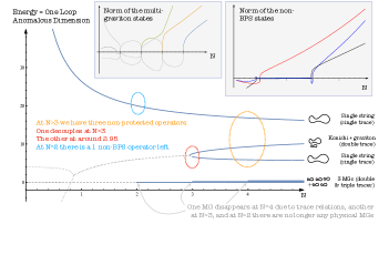
Figure 1: At large $N$ there are 3 MGs and 3 non-protected states. This counting persists for all $N\geq 6$. As we decrease $N$ some of these states start decoupling (drawn as dashed lines in the figure) due to trace relations. At $N=2,3,4$ we have $1,3,5$ physical states respectively – with a positive norm and non-negative energy.

In figure 1 we find complex and negative energies. Aren’t these the eigenvalues of a positive definite Hermitian operator $H=\{Q,Q^{\dagger}\}$ which should thus only have positive eigenvalues? What is going on?

The solution to this small puzzle is that trace relations are kicking in and saving us from non-unitarity contradictions. As discussed above, a convenient object to automatically encode these relations is the Wick contraction matrix $\mathbb{W}$ which in this case is a simple $6\times 6$ matrix

$$\!\!\!\mathbb{W}\!=\!\!\footnotesize\left(\!\!\begin{array}[]{ccc}4N^{6}\!-\!4N^{4}\!+\!36N^{2}\!-\!36&6N^{6}\!+\!14N^{4}\!+\!4N^{2}\!-\!24&\!\dots\\ 6N^{6}\!+\!14N^{4}\!+\!4N^{2}\!\!-\!24&14N^{6}\!+\!26N^{4}\!-\!24N^{2}\!\!-\!16&\!\dots\\ \vdots&\vdots&\!\ddots\end{array}\!\!\right)\!.$$ (12)

This is a symmetric real matrix so that the norm of any state $\mathbb{v}^{\dagger}\cdot\mathbb{W}\cdot\mathbb{v}$ is real and the eigenvalues of $\mathbb{W}$ are also real. At large $N$ they are all positive but as we decrease $N$ we see that the norm of the non-protected states can become negative or even vanish in a finite $N$ segment. This second scenario can happen for states whose energy acquires an imaginary part as illustrated in the right-most inset in figure 1. In the second inset of that figure we plot the three eigenvalues of the $3\times 3$ restricted Wick matrix once we project it onto the MG degenerate subspace. Precisely at integers where trace relations kick in, some eigenvalues of this matrix disappear and the corresponding states become unphysical.

In sum: if we stick to integer $N$’s and systematically throw away unphysical states which drop out due to trace relations then all energies and norms will be nice non-negative real numbers. If, on the other hand, we keep all states and allow $N$ to take continuous values we gain a more unified description of the spectrum where many previously unrelated states become nicely connected.

IV The BH sector

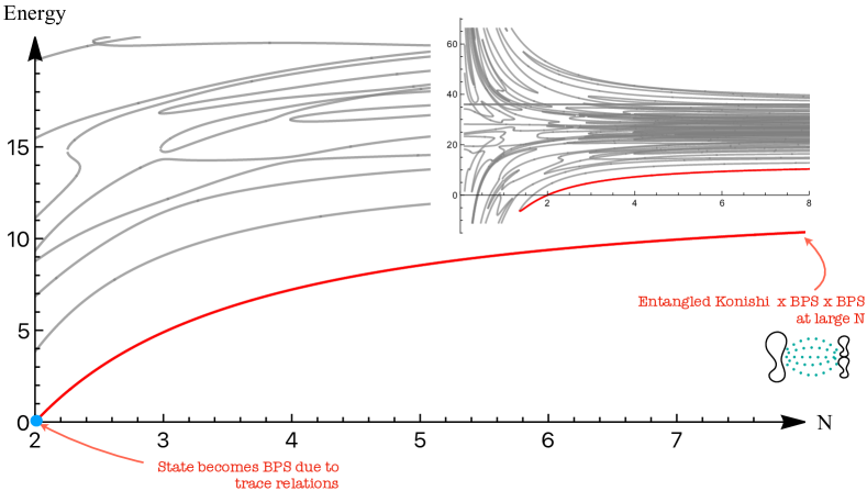
Figure 2: Energies of the 69 states in the BH sector described in the main text. There are several level repulsions (and some accidental crossings which will likely get resolved at two-loops, see Appendix D). Some things are similar to the two scalars toy example – for instance, states annihilating extremely close to integers where the trace relations kick in – but there is an obvious novelty here: There is a state whose energy goes to zero at $N=2$. This is the so-called $1/16$-th $N=2$ black hole state identified by the blue circle in the figure. This state flows to an entangled triple trace of a Konishi multiplet operator and two gravitons at large $N$ (14). The inset shows the same plot in a bigger range and interestingly the black hole annihilates with the second excited state – which is a single trace at large $N$ – a bit to the left of $N=1$.

Multiplets that correspond to BPS BHs cannot have identically vanishing energies for all $N$ – this is what distinguishes them from MGs. Together with analyticity of one-loop energies, this implies that a BH multiplet in the $SU(N_{0})$ theory must develop an anomalous dimension when $N$ is perturbed away from $N_{0}$. However, as we change the coupling while staying at $N=N_{0}$, the multiplet is expected to remain short Grant et al. (2008); Chang and Lin (2023).

One possible scenario is as follows. Assuming that the representation continues to be unitary away from $N_{0}$, the BH multiplet recombines with another short multiplet (which is killed by $SU(N_{0})$ trace relations). Such BPS BH multiplets lie at the unitarity threshold and satisfy shortening conditions $A_{1}$ or $A_{2}$ Cordova et al. (2019); Dolan and Osborn (2003) (see Appendix E). The simplest BH multiplet discussed below, and all others found in Choi et al. (2023) are of the type $A_{1}\bar{L}$ and seem to realize this scenario. It would be interesting to investigate if there are examples of BH multiplets which become non-unitary away from $N_{0}$.

Recently in Chang and Lin (2023), the first non-MG cohomology was found in the $SU(2)$ theory. Its quantum numbers are given by (1) with $n=0$. With these quantum numbers, at tree level, the operators are made out of letters without $SU(2)_{R}$ dotted indices, see Appendix A. At large $N$, there are a total of 8013 multi-trace operators with these quantum numbers. We can reduce the number of states we are dealing with, by imposing certain conditions: The BH is a primary under $\textrm{psu}(1,2|3)$ and it is a singlet under the unbroken $SU(3)$ of R-symmetry $SO(6)\sim SU(4)$ (if this were not the case, we should have seen additional non-MG states at this level in the exhaustive search of Chang and Lin (2023)). We thus impose

$$S^{i}_{+}\lvert\psi\rangle =0\ ,\,i=1\ldots 3$$

$$R_{i}^{j}\lvert\psi\rangle =0\ ,\,i\neq j,\ i,j=1,\ldots,3\,,$$ (13)

where in the first line, we only require that the classical $S$’s kill the states. These constraints commute with the action of $H$. We can further separate the states in this subspace by their parity (8) – there are 69 parity even states and 30 parity odd states. Diagonalizing the mixing matrix $\mathbb{H}$ in the parity even sector, gives us the anomalous dimensions in figure 2. The lowest energy trajectory in this sector corresponds to the BH. As anticipated above, the state becomes $\tfrac{1}{16}$-BPS at $N=2$ because a part of the multiplet becomes null due to $N=2$ trace relations. At $N=2$ it is given by (2). At large $N$, it takes the form of an interesting entangled triple trace,

$$\underbrace{\left(\operatorname{tr}fX+\operatorname{tr}\psi^{3}\psi^{2}\right)^{2}}_{\text{BPS}\times\text{BPS}}\overleftrightarrow{\mathbf{E}}_{1}\underbrace{(\operatorname{tr}ZY\psi^{1}-\operatorname{tr}YZ\psi^{1})}_{\text{Konishi}}+\texttt{cyclic}\ .$$ (14)

On the left, we have (a product of) two gravitons and on the right we have a Konishi (multiplet operator). The entangling operator $\overleftrightarrow{\mathbf{E}}_{1}$ adds some charges on the right and removes the same ones from the left. For example, it will contain a term $\tfrac{1}{6}\overleftarrow{S^{1}}\otimes\overrightarrow{Q_{1}}$ where $Q_{1}$ acts on the right and its conjugate $S^{1}$ acts on the left. For compactness we will write it as $\frac{1}{6}Q_{1}$ leaving implicit the conjugate action on the left. The full entanglement operator is then

$$\overleftrightarrow{\mathbf{E}}_{1}= 1+\tfrac{1}{6}Q_{1}+\tfrac{1}{2}Q_{2}+\tfrac{1}{2}Q_{3}-\tfrac{1}{12}Q_{2}Q_{1}-\tfrac{1}{12}Q_{3}Q_{1}-\tfrac{1}{6}Q_{3}Q_{2}-\tfrac{1}{2}R_{1}^{2}-\tfrac{1}{4}R_{1}^{2}Q_{3}+\tfrac{1}{36}R_{1}^{2}Q_{3}Q_{2}+\tfrac{1}{24}R_{1}^{3}Q_{1}Q_{3}+$$ (15)

$$\tfrac{1}{36}R_{1}^{3}Q_{2}Q_{3}+\tfrac{1}{24}R_{2}^{3}R_{1}^{2}Q_{3}+\tfrac{1}{24}R_{3}^{2}R_{1}^{3}Q_{2}+\tfrac{1}{24}Q_{2}Q_{3}R_{1}^{3}+\tfrac{1}{24}Q_{3}Q_{2}R_{1}^{2}-\tfrac{1}{216}R_{1}^{3}R_{1}^{2}Q_{3}Q_{2}-$$

$$\tfrac{1}{48}R_{3}^{1}Q_{3}R_{1}^{3}R_{1}^{3}+\tfrac{1}{72}Q_{3}Q_{2}R_{1}^{2}Q_{1}-\tfrac{1}{36}Q_{3}Q_{2}Q_{1}-\tfrac{1}{48}R_{2}^{1}Q_{2}R_{1}^{2}R_{1}^{2}+\tfrac{1}{24}R_{3}^{1}R_{2}^{1}R_{1}^{3}R_{1}^{2}Q_{1}\ ,$$

where $Q_{i}\equiv Q_{i-}$, $\overleftrightarrow{\mathbf{E}}_{2}$ and $\overleftrightarrow{\mathbf{E}}_{3}$ are defined by cyclically changing $1\rightarrow 2\rightarrow 3\rightarrow 1$, and each term is implicitly multiplied by its conjugate (obtained by $Q_{i}\rightarrow S^{i}$ and $R^{a}_{b}\rightarrow R^{b}_{a}$ and flipping the order of operators) acting on the left.

Perhaps the most famous quantum state, the EPR state, can be nicely entangled in a similar fashion,

$$\lvert\uparrow\rangle\overleftrightarrow{\mathbf{e}}\lvert\downarrow\rangle=\lvert\uparrow\downarrow\rangle+\lvert\downarrow\uparrow\rangle\,,\qquad\overrightarrow{\mathbf{e}}=1+\overleftarrow{\sigma_{-}}\otimes\overrightarrow{\sigma_{+}}\,,$$ (16)

which is what motivated us to dub $\overleftrightarrow{\mathbf{E}}$ as the entanglement operator. Amusingly, in the previous section we encountered Konishi dressed by gravitons as well but a key difference is that there is no entanglement in (11) while there is a huge amount in (14).

A cute – albeit useless – graphical representation of the BH state at $N=2$ and $N=\infty$ is given in Appendix H.

V The $1/16$-th BH Fate

We could now try to follow the large $N$ state (14) to large $\lambda$. Here we have to be careful.

The easy thing to do is to follow the state to strong coupling at $N=\infty$. This corresponds to free strings whose energies are additive so that the energy of the state (14) is equal to the energy of Konishi plus the energy of the two gravitons. It is thus given by $19/2+\gamma_{\texttt{Konishi}}(\lambda)$ because only Konishi develops an anomalous dimension. Using integrability, $\gamma_{\texttt{Konishi}}(\lambda)$ can be followed all the way from weak to strong coupling Gromov et al. (2010). At weak coupling it is given by $12\lambda+\dots$ while at strong coupling it behaves as $2\lambda^{1/4}-4+2/\lambda^{1/4}+\dots$ Gubser et al. (1998); Arutyunov et al. (2004); Gromov et al. (2010). In sum, if we follow our black hole state (14) to strong coupling at infinite $N$ we end up at a heavy state with energy

$$E_{\texttt{Integrability}}=2\lambda^{1/4}+11/2+\dots$$ (17)

as depicted by the solid red line in figure 3.

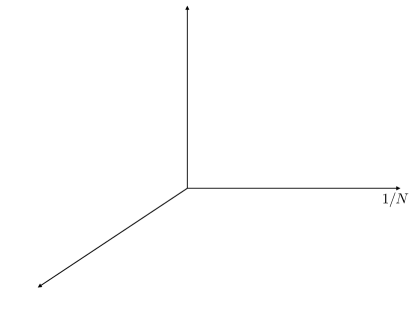
Figure 3: At $N=2$ the BH state is a $1/16$-BPS state whose energy is zero at any coupling (blue line). The green line is a sketch of the weak coupling interpolation in section IV. At infinite $N$ the BH state is a triple trace state made of Konishi and two gravitons. As we crank up the coupling at infinite $N$, the anomalous dimension follows Konishi Gromov et al. (2010) (red solid line). If we stick to large but finite $N$ as we go to strong coupling, the state will probably follow a stair-case pattern like figure 4 and eventually plateau at an approximate MG state (dashed red line). The energy at strong coupling will be a finite integer away from the classical dimension $19/2$ of the BH state. Then, if we follow the state to small $N$ it should again dive to zero at $N=2$ as depicted by the dotted pink line; it would be important to find a new idea which would allow us to say something quantitative about this strong coupling interpolation.

The harder – but somewhat more accurate – thing to do is to follow the state at large but finite $N$. The final result can be dramatically different since at finite $N$ strings will no longer be free, integrability is broken, and level repulsion will dramatically affect the fate of the various states. The point is that there are two families of states which will clearly cross at infinite $N$:

• Products of protected operators, i.e. operators like $\operatorname{Tr}(ZZ)\operatorname{Tr}(\bar{Z}\bar{Z})$. At infinite $N$, and for any coupling, these operators will have no anomalous dimension. At large but finite $N$ they acquire a small binding energy $\gamma(\lambda)$ of order $1/N^{2}$. They are schematically depicted as the red dotted lines in figure 4. They are MG-like states.

• Products involving at least one non-protected state such as Konishi – such as our state (14). As soon as a state involves at least one non-protected state (dual to an excited string) its energy will grow as $\lambda^{1/4}$ at infinite $N$ as described in the previous paragraph, see (17). These states are represented by the blue solid lines in figure 4. They necessarily cross many red dotted lines at finite values of $\lambda$.

At large but finite $N$ the level crossing will be resolved by nonperturbative mixing Korchemsky (2016) as sketched on the right panel of figure 4. A small excited string at weak coupling like Konishi – or Konishi dressed by a bunch of other strings as in our case (14) – will therefore not grow into a heavy massive excited string with huge energy at strong coupling but instead end up as a MG-like state after some level repulsion(s). In sum, at large but finite $N$ we expect our state to end up as a MG-like state with an energy some finite integer distance away from its weak coupling energy $19/2$,

$$E_{\text{\textst{{Integrability}}}}=19/2+\texttt{integer}\,$$ (18)

as sketched by the dashed red line in figure 3.

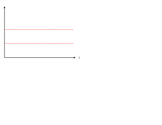
Figure 4: On the left cartoon, the blue solid lines represent the planar dimensions of non-protected states – whose energy blows up at strong coupling – and the red dashed lines correspond to products of protected traces (gravitons). At large but finite $N$ mixing will resolve the level crossing and we end up with something as sketched on the right. (Not all horizontal lines get repelled - some stay protected by SUSY and those are precisely the MGs; we are not drawing those.)

One could be puzzled: How can it make such a difference to follow the state to strong coupling at huge $N$ versus infinite $N$? It depends what we mean by follow. If we imagine a real experimental setup where we slowly tune the coupling in time, interpolating between weak and strong coupling, then we would stay in the lowest energy state – the dashed line in figure 3 – if we move slowly enough. If we move too fast, we will jump levels and follow the integrability prediction – the solid red line. The larger $N$, the slower we would need to move nearby a level repulsion to stay in the lowest level, see Appendix G for an illustrative toy model.

VI Discussion

Once we convert gauge theory computations into loop diagrammatics where the number of colours shows up as a simple weight factor, we can take it to be $N=3.14159$ or any other value. This can be useful if we want to follow adiabatiacally operators across $N$ from regimes where we understand them very well (the integrable $N\to\infty$ corner for example) all the way to more challenging domains.

We used this idea to provide a new perspective on the lightest of the recently discovered non-multigraviton $1/16$-BPS cohomologies, sometimes simply called the (lightest) black hole state. At weak coupling, it is a protected state with zero anomalous dimension at $N=2$ while at large $N$ it is a non-trivial, very entangled, triple trace state dual to a Konishi string plus two gravitons.

Was this expected? Is it more natural that the BH comes from such a “maximally fragmented” triple trace product of light strings instead of a single large string? Should we expect something similar for the other recently found BHs Choi et al. (2023)? Will the $n=1$ state in (1) flow to a quadruple trace with one small non-protected string dressed by three gravitons?

What about $N>2$ black holes? It would be interesting to find a BH state for $N=3$ and follow it again in $N$. An interesting question is whether it will remain a 1/16-BPS BH at $N=2$. Naively this seems plausible: decreasing $N$ further from $3$ to $2$ corresponds to increasing the gravitational force further so why would the black hole go away? If that is the case, its energy should decrease to zero at $N=3$ from the right but then, instead of going negative – and decoupling from the theory – it should have have a double zero there, jump back up to dive back to zero one unit to the left again, at $N=2$. It would be very cool to see this happen! It would also be very interesting to continue the superconformal index in $N$ (possibly using recent advances in the giant graviton expansion Gaiotto and Lee (2021); Imamura (2021); Choi et al. (2022b)) – what happens to the BH contribution at non-integer $N$?

We also discussed the fate of the BH state as we move both to large $N$ and strong coupling. We argued that if we move slow enough we end up with a gas of gravitons at strong coupling (four gravitons for the lightest BH studied in this note) but if we move quickly we will end up with a very massive small string (the Konishi string) dressed by two gravitons, see figure 3. As depicted there, there should also be an interpolation line across many $N$’s at strong coupling. It would be fascinating to try to work it out. Perhaps some localization examples could be a good starting point to develop some intuition.

Finally, we should probably not be obsessed with the BPS states as far as black hole physics goes. What we are calling the BH state, the lowest curve in 2, is a priori not more of a black hole than any of the other energy levels. In Appendix H we started a simple exploration of these other states and their statistics. We find that the correlation functions with simple probes of these states lie close to typicality, as expected for heavy states Balasubramanian et al. (2005, 2008). It would be very interesting if we could make contact between the finite $N$ partition function of Aharony et al. (2004); Kristensson and Wilhelm (2020) and some of the physics of non-supersymmetric BHs such as those found by Chong, Cvetic, Lu and Pope Chong et al. (2005), from a microscopic description of these objects as quantum operators in maximally supersymmetric gauge theory.

Appendix A Notation and Conventions

The field content of $\mathcal{N}=4$ SYM consists of the following fields in the adjoint of $SU(N)$: six real scalars $\phi^{ij}$, four chiral and four anti-chiral fermions $\Psi^{i}_{\alpha}$ and $\bar{\Psi}_{i\dot{\alpha}}$ and the gauge bosons $\mathcal{A}_{\mu}$. The R-charge indices take the values $i,j=1\ldots 4$, and the $SU(2)_{L}$ and $SU(2)_{R}$ Lorentz indices $\alpha,\dot{\alpha}=\pm$. We can define the self-dual and anti self-dual field strengths $\mathcal{F}_{\alpha\beta}$ and $\mathcal{\tilde{F}}_{\dot{\alpha}\dot{\beta}}$.

In this paper, we consider 1/16-BPS operators. Let $Q\equiv Q_{4-}$ and $S\equiv S^{4-}$ be the charges that kill them. Such operators must be made out of the following BPS letters, each of which is killed by the classical action of $Q$ and $S$,

• $(X,Y,Z)\equiv\phi_{4i}=\tfrac{1}{2}\epsilon_{4ijk}\phi^{jk}$,

• $\psi^{i}=\Psi^{i}_{+}$ and $\lambda_{\dot{\alpha}}=\bar{\Psi}_{4\dot{\alpha}}$,

• $f=\mathcal{F}_{++}$,

• Covariant derivatives $D_{+\dot{\alpha}}$ .

At one-loop, $Q$ acts on the BPS letters as follows,

$$\{Q,\psi^{m}\} = -i\epsilon^{mnp}[\phi_{4n},\phi_{4p}]$$

$$\left[Q,f\right] = i[\phi_{4n},\psi^{n}]$$

$$\left[Q,D_{+\dot{\alpha}}\right] = -i[\lambda_{\dot{\alpha}},\ \}\,.$$ (19)

There is a smaller subspace in which we can look for 1/16-BPS operators – we restrict to operators which have no $SU(2)_{R}$ indices (i.e. no $\dot{\alpha}$’s). It is built out of the following seven letters

$$\mathcal{W}_{A}=\{X,Y,Z,\psi^{1},\psi^{2},\psi^{3},f\}\,.$$ (20)

This subspace is closed at one-loop because the Beisert Hamiltonian only shuffles the indices around and does not add new ones. We call this the “No derivative sector”. The black hole discussed in the main text lies within it.

Appendix B Non-planar H – Indices and Signs

In Beisert (2004), the one-loop Hamiltonian was written down. However, there are some sign ambiguities which were not completely spelled out – see footnote 1, Chapter 3 of Beisert (2004). Since we are forced to include all the letters in (20) to find 1/16-BPS states, we need to fix all the signs.

The scaling dimensions of the generators of the psu$(2,2|4)$ do not receive quantum corrections. So, for algebra generators $\mathfrak{g}$, we have

$$\left[\delta D(g_{\text{YM}}),\mathfrak{g}(g_{\text{YM}})\right] = 0\ ,$$

$$\implies g_{\text{YM}}^{2}\left[D^{(2)},\mathfrak{g}^{(0)}\right] = 0\ .$$ (21)

In other words, $H$ commutes with the classical generators. By imposing this condition, we fixed the sign ambiguities and ended up with the following expression for $H$,

$$H=\sum_{A,B,C,D}\mathcal{C}_{AC}^{BD}(-)^{BC}(-)^{BD}:\operatorname{tr}[\mathcal{W}_{A},\check{\mathcal{W}}^{B}\}[\mathcal{W}_{C},\check{\mathcal{W}}^{D}\}:$$

Let us now work out a simple example that shows how to work with the dilatation operator. Consider the rank one sector $SU(1|1)$ that consists of one boson, say $Z\equiv\phi^{12}$, and one fermion, say $\psi\equiv\Psi^{1}_{+}$. In this sector, the coefficient $\mathcal{C}_{AC}^{BD}$ in (3) is simply a super-permutation, i.e.,

$$\mathcal{C}_{Z\psi}^{Z\psi}=\mathcal{C}_{\psi Z}^{\psi Z}=-\mathcal{C}_{Z\psi}^{\psi Z}=-\mathcal{C}_{\psi Z}^{Z\psi}=\tfrac{1}{2}\mathcal{C}_{\psi\psi}^{\psi\psi}=1\,.$$ (22)

Plugging these into (3), we get the following form for $H$ in this subsector

$$H=\frac{-2}{N}\left(\operatorname{tr}[Z,\psi][\check{Z},\check{\psi}]-2\operatorname{tr}\left(\psi\psi\check{\psi}\check{\psi}\right)\right)\,.$$ (23)

Consider the action of $H$ on the state $\operatorname{tr}(\psi\psi Z)$. For ease of illustration, let us consider the dilatation operator in the $U(N)$ theory. The propagator in this case is just the first term in (4). The first term in (23), $\operatorname{tr}(Z\psi\check{Z}\check{\psi})$, acts on the state as,

(24)

where the lines connecting letters represent contraction of gauge indices within a trace and the orange dashed lines are from the propagator. The letters in red and blue are from the Hamiltonian and the state respectively. The minus sign in the second line comes from moving $\check{\psi}$ across $\psi$ to act on the second letter.

The action of the Hamiltonian is the same for both $SU(N)$ and $U(N)$. (The trace term cancels in the commutator. See Beisert (2004) for a discussion.) In the $SU(N)$ theory, the trace of any single letter is zero so the RHS of (24) ends up being $-N\operatorname{tr}(\psi\psi Z)$. Similarly, adding up the contributions from all the terms of $H$, we get

$$H\cdot\operatorname{tr}\left(\psi\psi Z\right)=12\operatorname{tr}\left(\psi\psi Z\right)\,.$$ (25)

Not only is the action on this trace very simple, but it actually yields back the same state in this example with the famous energy $12$ which keeps showing up in this note. That is because $\operatorname{tr}(\psi\psi Z)$ is yet another manifestation of the famous Konishi multiplet, this time in the form of the so-called $SU(1|1)$ Konishi representative.

Appendix C $SU(2)$ Details

The $SU(2)$ NHW basis comprises two single traces, three double traces and one triple trace:

$$\!\!\!\!\!\!\mathbb{v}_{1}=\operatorname{tr}(Z^{3}X^{3})-\operatorname{tr}(ZX)^{3},$$

$$\!\!\!\!\!\!\mathbb{v}_{2}=\operatorname{tr}(Z^{2}XZX^{2})+\operatorname{tr}(Z^{2}X^{2}ZX)-2\operatorname{tr}(ZX)^{3},$$

$$\!\!\!\!\!\!\mathbb{v}_{3}=\operatorname{tr}(X^{3})\operatorname{tr}(Z^{3})-\operatorname{tr}(ZX^{2})\operatorname{tr}(Z^{2}X),$$

$$\!\!\!\!\!\!\mathbb{v}_{4}=\operatorname{tr}(Z^{2})\operatorname{tr}(ZX^{3})+\operatorname{tr}(X^{2})\operatorname{tr}(Z^{3}X)-$$

$$\qquad\qquad\qquad\qquad-2\operatorname{tr}(ZX)\operatorname{tr}(ZXZX),$$

$$\!\!\!\!\!\!\mathbb{v}_{5}=\operatorname{tr}(ZX)\operatorname{tr}(Z^{2}X^{2})-\operatorname{tr}(ZX)\operatorname{tr}(ZXZX),$$

$$\!\!\!\!\!\!\mathbb{v}_{6}=\operatorname{tr}(X^{2})\operatorname{tr}(Z^{2})\operatorname{tr}(ZX)-(\operatorname{tr}(ZX))^{3}\,.$$ (26)

Let us check that one of its elements – the first say – is indeed killed by acting twice with the raising operator:

$$\mathbb{v}_{1}\!\!\!\! ={\color[rgb]{1,0,0}1}\operatorname{tr}(ZZZXXX)\!-\!{\color[rgb]{0,0,1}1}\operatorname{tr}(ZXZXZX)$$

$$(J_{+})\cdot\mathbb{v}_{1}\!\!\!\! ={\color[rgb]{1,0,0}2}\operatorname{tr}(ZZZZXX)\!+\!({\color[rgb]{1,0,0}1}-{\color[rgb]{0,0,1}3})\operatorname{tr}(ZZZXZX)$$

$$(J_{+})^{2}\cdot\mathbb{v}_{1}\!\!\!\! =2\!\times\!2\operatorname{tr}(ZZZZZX)\!+\!(1-3)\!\times\!2\operatorname{tr}(ZZZZZX)$$

$$=0\,.$$

Note that we did not include in the NHW basis (26) the highest-weight states which would be killed by a single action of the raising operator as those would form a closed block by themselves. In other words, the NHW basis (26) is made of those operators who are one unit away from being HW.

In this sector, the Hamiltonian takes the simple form

$$H=\frac{-2}{N}\operatorname{tr}[Z,X][\check{Z},\check{X}]\,.$$ (27)

At large $N$, the strings become free and states with different numbers of traces do not mix. The eigenstates in the NHW basis at large $N$ are as follows. There are two massive single traces,

$$|\psi\rangle^{N=\infty}_{\gamma=10\pm 2\sqrt{5}}=2\mathbb{v}_{2}-(3\mp\sqrt{5})\mathbb{v}_{1}$$

and a double trace made out of a Konishi $SU(2)$ representative dressed by a $1/2$-BPS 20’ operator (a single graviton)

$$|\psi\rangle^{N=\infty}_{\gamma=12}=\mathbb{v}_{5}=|\texttt{graviton}\rangle\times|\texttt{su(2) konishi}\rangle\,.$$ (28)

The following states at large $N$ are the multigravitons,

$$|\psi\rangle^{N=\infty}_{\gamma=0}=\begin{cases}\mathbb{v}_{3}&\\ \mathbb{v}_{6}&\\ -3\mathbb{v}_{4}+4\mathbb{v}_{5}&\end{cases}\,.$$ (29)

It is instructive to recall how the Wick contraction matrix is computed. Consider $\mathbb{W}_{11}$ given by the wick contraction of two $\mathbb{v}_{1}$’s. At leading order at large $N$ we have that the Wick contraction matrix will be dominated by the planar contributions $\mathbb{W}_{11}\simeq\langle\mathbb{v}_{1}\mathbb{v}_{1}\rangle_{\texttt{planar}}$ given by

(30)

We can replace each propagator here by the $SU(N)$ propagator given by the right hand side of (4),

(31)

to get

(32)

where we used the second term of the propagator once; using it more times leads to more suppressed terms in $1/N$ inside the dots. Once we transformed Wick contractions into pictures like this all we need to do is assign a factor of $N$ for each colour loop. The first term has six loops and is thus leading while the second term has five loops; all in all we see that

$$\langle\mathbb{v}_{1}\mathbb{v}_{1}\rangle_{\texttt{planar}}=4N^{6}-24N^{4}+O(N^{2})\,.$$ (33)

Note that the leading term perfectly matches the leading term in the first element of the Wick contraction matrix $\mathbb{W}$ in (12); to match the other ones we would need to add to this computation the other non-planar Wick-contractions as well which kick in at order $N^{4}$.

Appendix D Level Crossing Lift at Two-Loops

Sometimes levels still cross at finite $N$ as we can see in figure (2). This is an accidental remnant of integrability, and at higher loops we expect all such crossings to be resolved. As illustration we consider here a simple $SU(2)$ sector example where levels cross at one loop but such crossing is then nicely lifted at two loops.

Consider the subspace in the $SU(2)$ sector that

• is made out 5 $Z$’s and 3 $X^{\prime}s$,

• is NHW, i.e., killed by $J_{+}^{2}$ but not by $J_{+}$, and,

• has even parity.

There are nine states in this invariant subspace. As before, we can compute the one-loop anomalous dimensions of these states using (3). They are the gray lines of figure 5. The third and fourth energy levels cross at $N\sim 4.3$ as clearly seen in the inset.

The dilatation operator in the $SU(2)$ sector is known at two-loop order Beisert et al. (2003a); Kim et al. (2003). It takes the following form,

$$H_{2} = \frac{4}{N}:\operatorname{tr}[Z,X][\check{Z},\check{X}]:+$$ (34)

$$\frac{2}{N^{2}}:\operatorname{tr}[Z,X][\check{Z},[Z,[\check{Z},\check{X}]]]:+$$

$$\frac{2}{N^{2}}:\operatorname{tr}[Z,X][\check{X},[X,[\check{Z},\check{X}]]]:$$

Now, diagonalizing the operator $H+\epsilon H_{2}$, we find the corrected spectrum, shown in figure 5 for a small $\epsilon=0.01$ in orange. As seen in the inset, the levels no longer cross but are instead repelled.

The levels crossings in figure 2 are also expected to be resolved at higher loops in a similar fashion. However, we cannot check this in a straightforward manner because the two-loop non-planar Hamiltonian for the general psu$(2,2|4)$ sector is not known.

Finally, note that the dilatation operator $\mathbb{H}$ could in principle become non-diagonalizable at non-integer N when there are coincident eigenvalues i.e. level-crossings. Since we expect accidental crossings to be resolved at higher loops as illustrated here, we do not worry about this possibility.

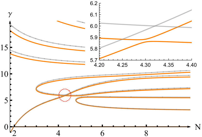
Figure 5: The gray lines are the one-loop anomalous dimensions and the orange lines are the eigenvalues of $H+\epsilon H_{2}$ for $\epsilon=0.01$. There is an accidental one-loop level crossing, highlighted by the dashed red circle. At two-loops, the levels are instead repelled as seen in the inset.

Appendix E Shortening Conditions

We review the short unitary representations of the $\text{su}(2,2|4)$ superconformal algebra Cordova et al. (2019); Dolan and Osborn (2003).

When the classical charges of the superconformal primary (SCP) satisfy one of the so-called shortening conditions, certain state in the multiplet becomes null and the multiplet is cut short. In su$(2,2|4)$, there are three types of short multiplets w.r.t $Q$ denoted by $A_{1},A_{2}$ and $B_{1}$. The long multiplet is denoted by $L$. Analogously, under the action of $\tilde{Q}^{\dot{\alpha}}$, the multiplets are labelled by $\bar{L},\bar{A}_{1},\bar{A}_{2}$ and $\bar{B}_{1}$. The shortening conditions and the corresponding null states are listed in the table 1.

	SCP	UB $\Delta=...$	$Q$ Null State
$A_{1}$	$[J,\bar{J}]^{(R_{1},R_{2},R_{3})}_{\Delta}$	$2\!+\!2J\!+\!\sum\limits_{i}R_{i}$	$[J\!-\!\tfrac{1}{2},\bar{J}]^{(R_{1}+\tfrac{1}{2},R_{2}+\tfrac{1}{2},R_{3}+\tfrac{1}{2})}_{\Delta+\tfrac{1}{2}}$
$A_{2}$	$[0,\bar{J}]^{(R_{1},R_{2},R_{3})}_{\Delta}$	$2\!+\!\sum\limits_{i}R_{i}$	$[0,\bar{J}]^{(R_{1}+1,R_{2}+1,R_{3}+1)}_{\Delta+1}$
$B_{1}$	$[0,\bar{J}]^{(R_{1},R_{2},R_{3})}_{\Delta}$	$\sum\limits_{i}R_{i}$	$[\tfrac{1}{2},\bar{J}]^{(R_{1}+\tfrac{1}{2},R_{2}+\tfrac{1}{2},R_{3}+\tfrac{1}{2})}_{\Delta+\tfrac{1}{2}}$

Table 1: Shortening conditions w.r.t $Q_{\alpha}\equiv Q^{4}_{\alpha}$ reproduced from Cordova et al. (2019) in the notations of Appendix A. There are analogous shortening conditions w.r.t $\tilde{Q}_{\dot{\alpha}}$. For the $A_{1}$ multiplet, in the first line, $J\geq 1/2$. UB stands for Unitarity Bound.

Existence of the null state implies an existence of a (classically) $Q_{-}$-closed state inside the multiplet. For the multiplets of type $A_{1}$, the null state is

$$Q_{\alpha}\lvert\text{SCP}\rangle^{\alpha}=Q_{+}\lvert\text{SCP}\rangle_{-}-Q_{-}\lvert\text{SCP}\rangle_{+}\,.$$ (35)

From this, it follows that the following state must also be null:

$$Q_{-}Q_{+}\lvert\text{SCP}\rangle_{+} =-Q_{+}Q_{-}\lvert\text{SCP}\rangle_{+}$$ (36)

$$=-Q_{+}\left(Q_{+}\lvert\text{SCP}\rangle_{-}-Q_{\alpha}\lvert\text{SCP}\rangle^{\alpha}\right)$$ (37)

$$=Q_{+}Q_{\alpha}\lvert\text{SCP}\rangle^{\alpha}\,.$$ (38)

Therefore, $Q_{+}\lvert\text{SCP}\rangle_{+}$ is $Q_{-}$-closed. The BH states (1) are of this form.

One can check that the multiplets of type $A_{2}$ also contain a $Q_{-}$-closed state, which is again $Q_{+}\lvert\text{SCP}\rangle$. The SCP of the multiplet $B_{1}$ is itself $Q_{-}$-closed.

Whether the operators above remain $Q_{-}$-closed at quantum level, depends on whether the short multiplet recombines into a long multiplet and obtains an anomalous dimension.

Appendix F More Chaos, More “Black Holes”

In this appendix we want to find some simple evidence for the following:

• The so-called BH state – the state whose energy vanishes at $N=2$ – is pretty typical; the other states with non-vanishing energies behave similarly. They are not any less black-hole-like.

• MG states, however, exhibit a somewhat different qualitative behavior. They have bigger disintegration probabilities in line with the intuition that they are dual to gases of loosely connected gravitons of sorts, rather than compact BH-like objects.

• At large $N$ chaos decreases in agreement with the expectation that – at fixed quantum numbers – we will be describing a bunch of free strings governed by integrability once $N\to\infty$.

Of course, this is all quite qualitative – we are at weak coupling after all – and will be based on some simple statistical analysis of the various states obtained when diagonalizing the non-planar dilatation operator for states with the BH and MG small quantum numbers.

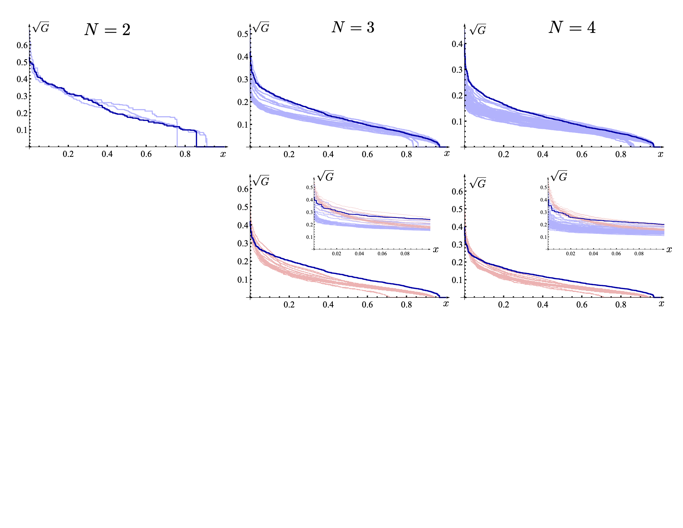
Figure 6: Correlators. BH’s in the top, MG’s in the bottom. MG have bigger disintegration $G$’s small $x$ region where these are bigger; otherwise the BH state is always (one of the) state(s) which disintegrates easier, i.e. with larger $G$.

The first evidence for the first two bullet points is represented in figure 6. On the top row of this plot we are depicting thousands of correlation functions per each of the $69$ states with the black hole quantum numbers while in the bottom row are are plotting the same correlation functions involving instead the $27$ multi-graviton states with that field content. With the field content of the BH state there are 8013 states. Out of these, 4893 are double or triple traces such as

$$\mathbb{v}_{i} = \operatorname{tr}(\psi^{3}\phi^{23})\times\operatorname{tr}(\phi^{13}\phi^{12})\times\operatorname{tr}(ff\phi^{12})$$ (39)

$$\equiv o_{1}(x)\times o_{2}(x)\times o_{3}(x)\,.$$

We can now take one of the $69$ states – lets call it $O_{A}$ – and study it disintegration into the constituents of these multi-traces. I.e. we take any $m$-trace basis element such as (39) and split it into $m$ single trace operators at different location to define

$$\mathbb{G}^{A}_{i}\equiv\langle O_{A}(0)o_{1}(x_{2})\dots o_{m}(x_{m})\rangle/(\mathcal{N}_{A}n_{1}\dots n_{m})$$ (40)

where $\mathcal{N}_{A}$ and $n_{i}$ are normalizations given by the operator two point functions. Finally, this quantity is not a number, it depends on the various locations $x_{j}$. To make it a number we assume these locations are the vertices of the basis of a regular pyramid whose tip is the origin and where all the vertices are one unit away from the tip so that the various propagators are just $1$. This is a very convenient definition because it is such that the extremal correlator (40) is directly computed by the $8013\times 8013$ Wick contraction matrix $\mathbb{W}$ defined in (6) as

$$G_{i}^{A}=\frac{(\mathbb{W}\cdot\psi^{(A)})_{i}}{(\psi^{(A)}\cdot\mathbb{W}\cdot\psi^{(A)})^{1/2}n_{1}\dots n_{m}}$$ (41)

where $O_{A}=\sum_{j}\psi_{j}^{(A)}\mathbb{v}_{j}$. The normalizations $n_{1}\dots n_{m}$ are computed similarly through Wick contractions but those are much simpler to compute since these are very small operators. For each $A=1\dots A_{\text{max}}$ we make a list of $G_{i}^{A}$ with $i$ ranging over the $i_{\text{max}}$ values corresponding to the basis elements which are either double or triple traces. Then we take the square root of the absolute value of each element and sort the list. We then define $x\equiv i/i_{max}\in[0,1]$ and plot the outcome. This is how we got the many blue lines in figure 6. For $N$ large enough there are $A_{max}=69$ blue curves each with $i_{max}=4893$ points but for low $N$ we have trace relations so that we will have less curves with less points. We can repeat this exercise for $O^{A}$ replaced by any one of the multigraviton states $O^{A}_{\text{MG}}$. This is how we got the red curves in the figure. As we can see in the figure, these correlation function show a nearly universal behavior and we expect deviations from typicality to be exponentially suppressed in the entropy Balasubramanian et al. (2005).

We like to think of (40) as a sort of decay process where the operator $O^{A}$ disintegrates into a bunch of $o_{1}\dots o_{m}$. We further like to imagine that this quantity being small is a sort of signal that the object is stable and does not want to be broken apart. Of all the blue curves, the BH state is, in this sense, among the most decay-prone ones at least for $N\geq 3$ where it clearly is close to the top of the pack of all states with those quantum numbers. Perhaps we should think of all these states as black holes of sorts and the one which becomes $1/16$-th BPS one at $N=2$ is in a way the least tight of all.

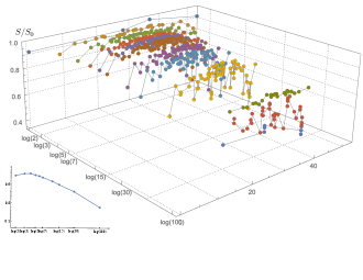
Figure 7: Eigenstates’ information entropies. At large $N$ (illustrated here with $N=100$) integrability kicks in and we see a big spread in the entropies indicating a sort of chaos breakdown; we also see that single (green), double (red) and triple (purple) traces start to cluster (which is why at that large $N$ only did we colour them differently). In the lower inset we averaged over the entropy in each $N$ cloud.

Multi-gravitons behave slightly differently it seems, for small $x$ corresponding to the most significant decay channels. As illustrated in the second row – most notably in the insets – for small values of $x$ they produce bigger decays $G$ compared to all blue states. Perhaps this is in line with the expectation that these should be some sort of graviton gases evoking a picture of a bunch of loosely right elements which one can easily tear apart?

Finally we went on to analyse the inner structure of the various $O_{A}$ states using the so-called information entropy content of the states, a nice quantity we learned from McLoughlin et al. (2023), a reference that we follow closely in the rest of this appendix. For each state $O_{A}$ we define a vector

$$\mathbb{w}_{A}\equiv\sum_{i}\psi_{i}^{(A)}\sqrt{\mathbb{W}}\cdot\mathbb{v}_{i}\equiv\sum_{i}c_{i}\mathbb{v}_{i}$$ (42)

Then the norm of the state is simply the usual scalar product, $\mathcal{N}_{A}=(\mathbb{w}_{A}\cdot\mathbb{w}_{A})^{1/2}=\sqrt{\sum_{i}|c_{i}|^{2}}$. Here the square root of the (real and symmetric) Wick contraction matrix is the matrix such that

$$\sqrt{\mathbb{W}}\cdot\sqrt{\mathbb{W}}=\mathbb{W}$$ (43)

which we can compute. (It is not completely trivial, it takes a few minutes for each $N$ choice with Mathematica using MatrixPower[W,1/2].)

The information entropy is then defined as

$$S\equiv-\sum_{i}\frac{|c_{i}|^{2}}{\mathcal{N}_{A}}\log\frac{|c_{i}|^{2}}{\mathcal{N}_{A}}$$ (44)

and the prediction is that a chaotic system should have an entropy consistent with Gaussian orthogonal ensemble random matrix theory. It should be well approximated by

$$S_{0}\equiv\log(I)+\log(2)+\gamma_{E}-2$$ (45)

where $I$ is the number of basis elements appearing in the sums (42) and (44) and $\gamma_{E}$ is the Euler’s constant. Indeed, if we plot $S/S_{0}$ for the various states at various values of $N$ we see that the ratio $S/S_{0}$ is indeed very close to $1$ as depicted in figure 7. In the figure’s inset we plotted, for each $N$ the average of $S/S_{0}$ over all states with the BH quantum numbers. We see that as we increase $N$ the system starts deviating from random matrix theory universality. This is expected as integrability should kick in. Indeed, at $N=100$ we see already that the ratio is around $0.7$ and – moreoever – the spread around this average is more pronounced with single, double and triple traces clustering around three separated clouds.

Physically this makes sense. If $N$ is very large compared to the various charges of the states, we are describing a bunch of free strings so their dynamics should indeed decouple into groups (depending on the number of strings) and each group should be simply described by order (integrability) rather than chaos.

Appendix G Adiabatic Toy Model

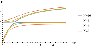
Figure 8: Eigenvalues of $\mathbb{H}(\lambda)$. The level splitting is smallest when $N$ is largest.

Consider the toy Hamiltonian

$$\mathbb{H}(\lambda)=\left(\begin{array}[]{cc}2&\frac{1}{N}\\ \frac{1}{N}&\frac{4\lambda}{1+\lambda}\\ \end{array}\right)$$ (46)

whose eigenvalues as function of $\lambda$ are plotted in figure 8. We see that $N$ controls how violent the level repulsion is: For large $N$ the levels only repel when they are extremely close to each other while for small $N$ the level repulsion is quite smooth.

We can now consider an experimental setup where $\lambda$ is allowed to grow with time as $\lambda=\beta t$ where $\beta$ is a positive constant that governs the growth rate. Smaller values of $\beta$ correspond to a slower ramp-up. We want to consider the time dependent Schrodinger equation

$$\frac{1}{i}\left(\begin{array}[]{c}\psi_{1}^{\prime}(t)\\ \psi_{2}^{\prime}(t)\end{array}\right)=\mathbb{H}(\lambda(t))\cdot\left(\begin{array}[]{c}\psi_{1}(t)\\ \psi_{2}(t)\end{array}\right)$$ (47)

(Note that as $t\to\infty$ the Hamiltonian asymptotes to a time independent Hamiltonian.) This is a nice toy model since this equation can be solved analytically.

(a)

(b)

Figure 9: Probability of staying in the lowest eigenvector of $\mathbb{H}(\lambda)$ when coupling reaches $\lambda=\beta t$ starting from the lowest eigenvector at $\lambda=0$.

We can start as the lowest energy eigenvector of $\mathbb{H}(0)$ as initial conditions and compute the probability of being in the lowest energy eigenvalue of $\mathbb{H}(\lambda)$ at any $t>0$, see figure 9. We see that at $N=16$, we need very small $\beta\sim 0.01$ in order to track the lowest energy state with high probability. On the other hand for the samller $N=2$, the probability is already very high at $\beta=0.25$. The larger the $N$, the slower we need to change $\lambda$ in order to track the lowest state. This makes sense because at large $N$ the levels get much closer which facilitates an easier crossing to the excited level.

If experimentalists were to continue the Konishi-plus-two-gravitons state (14) from weak to strong coupling at large $N$ in a similar fashion, they would encounter such level repulsions. Hasty experimentalists moving too fast will jump from level to level and follow the integrability prediction and end up with a very massive string state at strong coupling. Patient experimentalists moving very slowly (the larger $N$ the slower we would need to move) would stay in the lowest energy state and end up with a bunch of gravitons at strong coupling. These patient experimentalists would be following the true state as in this toy model.

Appendix H The State in Two Pictures

Written down in components (i.e. multi-traces) the states we are dealing why are intimidating – see figure 10. The large $N$ state with about 500 terms can be simplified to (14) using the entanglement operator while the $N=2$ state with its almost 8000 terms becomes compactified into the three-liner (2) once we take advantage of trace relations as well as the susy operator.

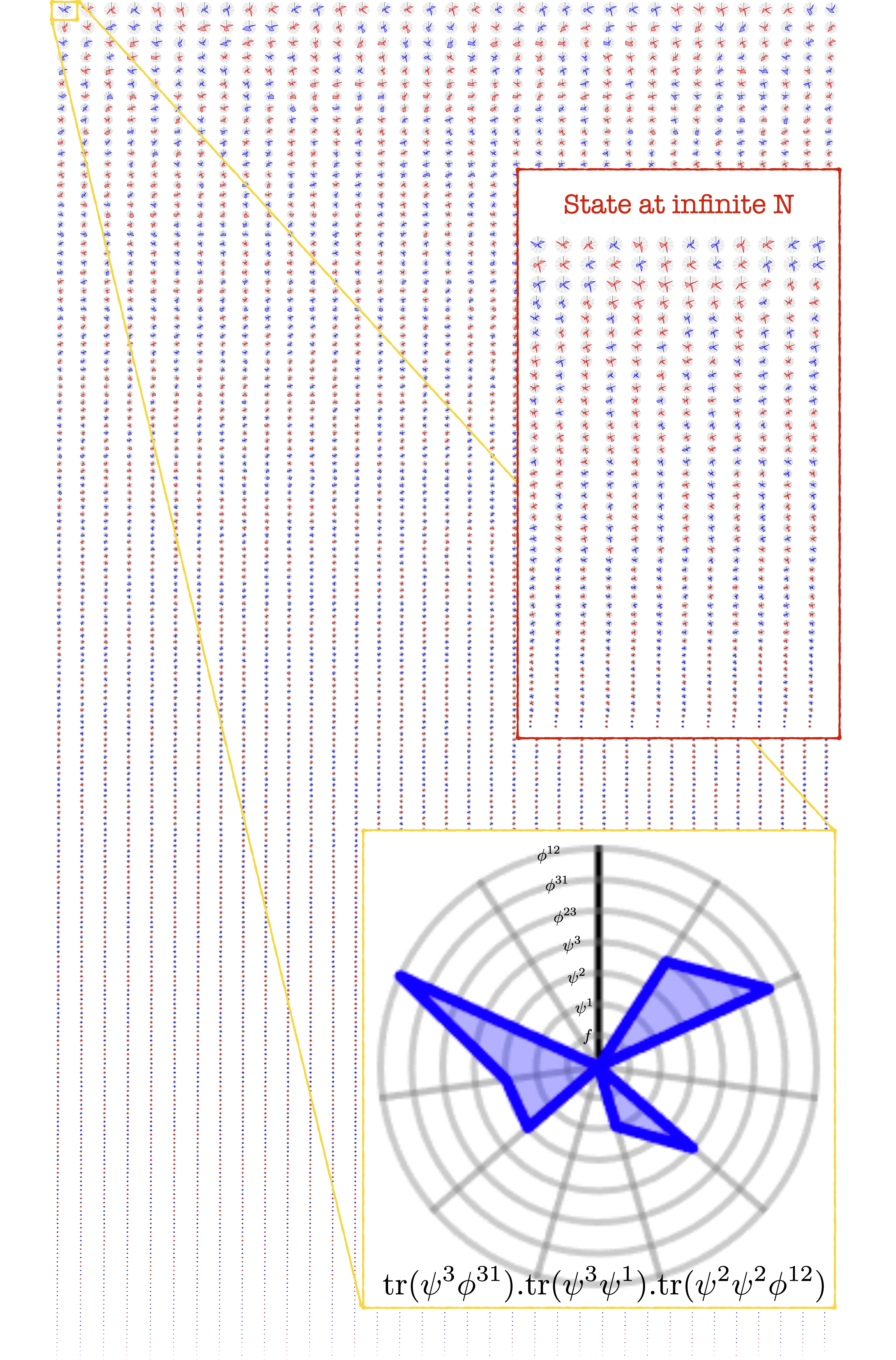
Figure 10: The black hole state for $N=2$ in the trace basis is huge while $N=\infty$ in the red box is much simpler. Each picture is given by a multi-trace following the example in the bottom. Each term is rescaled by square root of the amplitude of the corresponding multi-trace with red and blue indicating the sign of the amplitude.

References

- Chang and Yin (2013) Chi-Ming Chang and Xi Yin, “1/16 BPS states in 4 super-Yang-Mills theory,” Phys. Rev. D 88, 106005 (2013), arXiv:1305.6314 [hep-th] .
- Grant et al. (2008) Lars Grant, Pietro A. Grassi, Seok Kim, and Shiraz Minwalla, “Comments on 1/16 BPS Quantum States and Classical Configurations,” JHEP 05, 049 (2008), arXiv:0803.4183 [hep-th] .
- Gutowski and Reall (2004) Jan B. Gutowski and Harvey S. Reall, “Supersymmetric AdS(5) black holes,” JHEP 02, 006 (2004), arXiv:hep-th/0401042 .
- Kunduri et al. (2006) Hari K. Kunduri, James Lucietti, and Harvey S. Reall, “Supersymmetric multi-charge AdS(5) black holes,” JHEP 04, 036 (2006), arXiv:hep-th/0601156 .
- Chong et al. (2005) Z. W. Chong, Mirjam Cvetic, H. Lu, and C. N. Pope, “General non-extremal rotating black holes in minimal five-dimensional gauged supergravity,” Phys. Rev. Lett. 95, 161301 (2005), arXiv:hep-th/0506029 .
- Chang and Lin (2023) Chi-Ming Chang and Ying-Hsuan Lin, “Words to describe a black hole,” JHEP 02, 109 (2023), arXiv:2209.06728 [hep-th] .
- Choi et al. (2022a) Sunjin Choi, Seok Kim, Eunwoo Lee, and Jaemo Park, “The shape of non-graviton operators for ,” (2022a), arXiv:2209.12696 [hep-th] .
- Choi et al. (2023) Sunjin Choi, Seok Kim, Eunwoo Lee, Siyul Lee, and Jaemo Park, “Towards quantum black hole microstates,” (2023), arXiv:2304.10155 [hep-th] .
- Chang et al. (2023) Chi-Ming Chang, Li Feng, Ying-Hsuan Lin, and Yi-Xiao Tao, “Decoding stringy near-supersymmetric black holes,” (2023), arXiv:2306.04673 [hep-th] .
- Beisert (2004) Niklas Beisert, “The Dilatation operator of N=4 super Yang-Mills theory and integrability,” Phys. Rept. 405, 1–202 (2004), arXiv:hep-th/0407277 .
- Beisert et al. (2003a) N. Beisert, C. Kristjansen, and M. Staudacher, “The Dilatation operator of conformal N=4 superYang-Mills theory,” Nucl. Phys. B 664, 131–184 (2003a), arXiv:hep-th/0303060 .
- Janik (2002) Romuald A. Janik, “BMN operators and string field theory,” Phys. Lett. B 549, 237–244 (2002), arXiv:hep-th/0209263 .
- Beisert et al. (2003b) N. Beisert, C. Kristjansen, J. Plefka, and M. Staudacher, “BMN gauge theory as a quantum mechanical system,” Phys. Lett. B 558, 229–237 (2003b), arXiv:hep-th/0212269 .
- Casteill et al. (2007) P. Y. Casteill, R. A. Janik, A. Jarosz, and C. Kristjansen, “Quasilocality of joining/splitting strings from coherent states,” JHEP 12, 069 (2007), arXiv:0710.4166 [hep-th] .
- Gross et al. (2003) David J. Gross, Andrei Mikhailov, and Radu Roiban, “A Calculation of the plane wave string Hamiltonian from N=4 superYang-Mills theory,” JHEP 05, 025 (2003), arXiv:hep-th/0208231 .
- Binder and Rychkov (2020) Damon J. Binder and Slava Rychkov, “Deligne Categories in Lattice Models and Quantum Field Theory, or Making Sense of Symmetry with Non-integer ,” JHEP 04, 117 (2020), arXiv:1911.07895 [hep-th] .
- de Gennes (1972) Pierre-Gilles de Gennes, “Exponents for the excluded volume problem as derived by the wilson method,” Physics Letters A 38, 339–340 (1972).
- Fortuin and Kasteleyn (1972) Cornelius Marius Fortuin and Piet W Kasteleyn, “On the random-cluster model: I. introduction and relation to other models,” Physica 57, 536–564 (1972).
- Bargheer et al. (2019) Till Bargheer, Frank Coronado, and Pedro Vieira, “Octagons I: Combinatorics and Non-Planar Resummations,” JHEP 08, 162 (2019), arXiv:1904.00965 [hep-th] .
- Anninos et al. (2016) Dionysios Anninos, Thomas Hartman, and Andrew Strominger, “Higher spin realization of the ds/cft correspondence,” Classical and Quantum Gravity 34, 015009 (2016).
- Budzik et al. (2023) Kasia Budzik, Davide Gaiotto, Justin Kulp, Brian R. Williams, Jingxiang Wu, and Matthew Yu, “Semi-Chiral Operators in 4d Gauge Theories,” (2023), arXiv:2306.01039 [hep-th] .
- Cordova et al. (2019) Clay Cordova, Thomas T. Dumitrescu, and Kenneth Intriligator, “Multiplets of Superconformal Symmetry in Diverse Dimensions,” JHEP 03, 163 (2019), arXiv:1612.00809 [hep-th] .
- Dolan and Osborn (2003) F. A. Dolan and H. Osborn, “On short and semi-short representations for four-dimensional superconformal symmetry,” Annals Phys. 307, 41–89 (2003), arXiv:hep-th/0209056 .
- Marboe and Volin (2017) Christian Marboe and Dmytro Volin, “Fast analytic solver of rational Bethe equations,” J. Phys. A 50, 204002 (2017), arXiv:1608.06504 [math-ph] .
- Marboe and Volin (2018) Christian Marboe and Dmytro Volin, “The full spectrum of AdS5/CFT4 I: Representation theory and one-loop Q-system,” J. Phys. A 51, 165401 (2018), arXiv:1701.03704 [hep-th] .
- Marboe and Volin (2021) Christian Marboe and Dmytro Volin, “The full spectrum of AdS5/CFT4 II: Weak coupling expansion via the quantum spectral curve,” J. Phys. A 54, 055201 (2021), arXiv:1812.09238 [hep-th] .
- Gromov et al. (2010) Nikolay Gromov, Vladimir Kazakov, and Pedro Vieira, “Exact Spectrum of Planar Supersymmetric Yang-Mills Theory: Konishi Dimension at Any Coupling,” Phys. Rev. Lett. 104, 211601 (2010), arXiv:0906.4240 [hep-th] .
- Gubser et al. (1998) S. S. Gubser, Igor R. Klebanov, and Alexander M. Polyakov, “Gauge theory correlators from noncritical string theory,” Phys. Lett. B 428, 105–114 (1998), arXiv:hep-th/9802109 .
- Arutyunov et al. (2004) Gleb Arutyunov, Sergey Frolov, and Matthias Staudacher, “Bethe ansatz for quantum strings,” JHEP 10, 016 (2004), arXiv:hep-th/0406256 .
- Korchemsky (2016) G. P. Korchemsky, “On level crossing in conformal field theories,” JHEP 03, 212 (2016), arXiv:1512.05362 [hep-th] .
- Gaiotto and Lee (2021) Davide Gaiotto and Ji Hoon Lee, “The Giant Graviton Expansion,” (2021), arXiv:2109.02545 [hep-th] .
- Imamura (2021) Yosuke Imamura, “Finite-N superconformal index via the AdS/CFT correspondence,” PTEP 2021, 123B05 (2021), arXiv:2108.12090 [hep-th] .
- Choi et al. (2022b) Sunjin Choi, Seok Kim, Eunwoo Lee, and Jehyun Lee, “From giant gravitons to black holes,” (2022b), arXiv:2207.05172 [hep-th] .
- Balasubramanian et al. (2005) Vijay Balasubramanian, Jan de Boer, Vishnu Jejjala, and Joan Simon, “The Library of Babel: On the origin of gravitational thermodynamics,” JHEP 12, 006 (2005), arXiv:hep-th/0508023 .
- Balasubramanian et al. (2008) Vijay Balasubramanian, Bartlomiej Czech, Veronika E. Hubeny, Klaus Larjo, Mukund Rangamani, and Joan Simon, “Typicality versus thermality: An Analytic distinction,” Gen. Rel. Grav. 40, 1863–1890 (2008), arXiv:hep-th/0701122 .
- Aharony et al. (2004) Ofer Aharony, Joseph Marsano, Shiraz Minwalla, Kyriakos Papadodimas, and Mark Van Raamsdonk, “The Hagedorn - deconfinement phase transition in weakly coupled large N gauge theories,” Adv. Theor. Math. Phys. 8, 603–696 (2004), arXiv:hep-th/0310285 .
- Kristensson and Wilhelm (2020) Alexander T. Kristensson and Matthias Wilhelm, “From Hagedorn to Lee-Yang: partition functions of = 4 SYM theory at finite N,” JHEP 10, 006 (2020), arXiv:2005.06480 [hep-th] .
- Kim et al. (2003) Nakwoo Kim, Thomas Klose, and Jan Plefka, “Plane wave matrix theory from N=4 superYang-Mills on R x S**3,” Nucl. Phys. B 671, 359–382 (2003), arXiv:hep-th/0306054 .
- McLoughlin et al. (2023) Tristan McLoughlin, Raul Pereira, and Anne Spiering, “Quantum chaos in perturbative super-Yang-Mills Theory,” SciPost Phys. 14, 049 (2023).