Gravitational waves from phase transitions and cosmic strings in neutrino mass models with multiple Majorons

Abstract

We explore the origin of Majorana masses within the Majoron model and how this can lead to the generation of a distinguishable primordial stochastic background of gravitational waves. We first show how in the simplest Majoron model only a contribution from cosmic string can be within the reach of planned experiments. We then consider extensions containing multiple complex scalars, demonstrating how in this case a spectrum comprising contributions from both a strong first order phase transition and cosmic strings can naturally emerge. We show that the interplay between multiple scalar fields can amplify the phase transition signal, potentially leading to double peaks over the wideband sloped spectrum from cosmic strings. We also underscore the possibility of observing such a gravitational wave background to provide insights into the reheating temperature of the universe. We conclude highlighting how the model can be naturally combined with scenarios addressing the origin of matter of the universe, where baryogenesis occurs via leptogenesis and a right-handed neutrino plays the role of dark matter.

1 Introduction

The discovery of gravitational waves (GWs) [1] opens new opportunities to test physics beyond the standard model (BSM). This is particularly interesting for those models currently evading constraints from colliders and, more generally, from laboratory experiments. Even though GWs have so far been detected only from astrophysical sources, there are many different processes in the early universe that could lead to the production of detectable primordial stochastic GW backgrounds. In particular, a production from the vibration of cosmic strings [2] and from strong first order phase transitions [3, 4, 5] provide quite realistic and testable mechanisms within various extensions of the standard model (SM) [6, 7, 8].

These two GW production mechanisms are usually studied separately. In this paper we show how within the Majoron model [9], an extension of the SM explaining neutrino masses and mixing, a GW spectrum is produced where both sources can give a non-negligible contribution and fall within the sensitivity of planned experiments. In the Majoron model a type-I seesaw [10, 11, 12, 13, 14] Lagrangian results as the outcome of a global $U(1)_{L}$ spontaneous symmetry breaking and Majorana masses are generated by the vacuum expectation value (VEV) of a single complex scalar field. The massless Goldstone boson, identified as the imaginary part of the complex scalar, is dubbed as Majoron. The model can also nicely embed leptogenesis for the explanation of the matter-antimatter asymmetry of the universe [15].

The idea that a strong first order electroweak phase transition associated to the lepton number symmetry breaking can generate a stochastic GW background has been explored in [16]. In this case a coupling of the complex scalar to the SM Higgs field was considered. A phase transition within the dark sector of the Majoron model, disconnected from the electroweak phase transition, was considered in [17], where non-renormalisable operators and explicit symmetry breaking terms have been included in order to enhance the signal. Moreover, a low-scale phase transition, in the keV-MeV range was also considered in order to reproduce the NANOGrav putative signal at very low frequencies ($\sim 10^{-9}\,{\rm Hz}$) [18].

A first order phase transition from $U(1)_{L}$-symmetry breaking in the dark sector, with no coupling of the complex scalar field to the SM Higgs field, was also considered in [19] without resorting either to explicit symmetry breaking terms or to non-renormalizable operators. Both the case of low and high scale phase transition were explored. It was found that at low scales the NANOGrav result cannot be explained, unless one invokes some enhancement from some unaccounted new effect. On the other hand, it was found that at high energy scales the signal can be sufficiently large to fall within the sensitivity of future experiments such as $\mu$Ares [20], DECIGO [21], AEDGE [22], AION [23], LISA [24], Einstein Telescope (ET) [25], BBO [26] and CE [27]. However, this result relied on the introduction of an external auxiliary real scalar field undergoing its own phase transition occurring prior to the complex scalar field phase transition. Once the auxiliary scalar gets a VEV, its mixing with the complex scalar field generates a zero-temperature barrier described by a cubic term in the effective potential of the latter, leading to a strong first order phase transition and detectable GW spectrum.

In this paper, we show how the role of the auxiliary field can be nicely played by a second complex scalar in a multiple Majoron model. We discuss neutrino mass models with spontaneous breaking of multiple global lepton number symmetries, typically with hierarchical scales. The three right-handed (RH) neutrino masses are then generated by different complex scalars each undergoing its own independent phase transition occurring, in general, at different energy scales and breaking lepton number along a specific direction in flavour space. We have, then, what could be referred to as a (RH neutrino) flavoured Majoron model. Importantly, we show that a contribution from the vibration of cosmic strings generated from the spontaneous breaking of the global lepton number symmetry has also to be taken into account to derive the GW spectrum of these models. The overall spectrum then is the sum of contributions from both production mechanisms: a contribution from strong first order phase transitions and a contribution from the vibration of cosmic strings. For sufficiently strong phase transitions, the resultant signal looks like one or more peaks (from phase transition) over a slanted plateau (from cosmic string).

The paper is organised as follows. In Section 2 we review the traditional single Majoron model where the right-right Majorana mass term, with three RH neutrinos, is generated by a single complex scalar field breaking total lepton number symmetry. The differences in the Majorana masses are then to be ascribed to different couplings. Even in this traditional setup we point out that a GW production from the vibration of cosmic strings, not accounted for in previous works, should be considered and can give a detectable signal. In Section 3 we extend the model with an additional complex scalar with its respective global lepton number symmetry, whose spontaneous breaking gives mass to the two lighter RH neutrinos. In this way only two distinguished phase transitions occur with hierarchical energy scales. We show that the resulting GW spectrum is, in general, the sum of two contributions, one from the lower scale phase transition and one from the vibration of cosmic strings created at the highest scale symmetry breaking. The corresponding phase transition does not produce a sizeable contribution to the GW spectrum, but it results into a VEV of the complex scalar field that generates a term entering the effective potential describing the second phase transition at a lower scale. This term strongly enhances the production of GWs during the second phase transition. In this way the high scale complex scalar associated with the Majoron field provides the external auxiliary scalar that had to be assumed in [19], so that the model is self-contained and does not rely on external assumptions. Finally, in Section 4 we consider the case when all three RH neutrino masses are associated with different complex scalars, each charged under a different global lepton number symmetry. At high temperatures one has the restoration of a $U(1)_{L_{1}}\times U(1)_{L_{2}}\times U(1)_{L_{3}}$ symmetry. While the temperature decreases, a sequential breaking of each $U(1)_{L_{I}}$ symmetry occurs at a different scale accompanied by a different phase transition. In this case we show that the GW spectrum now can receive a contribution from both the two lower scale phase transitions and still from the vibration of cosmic strings at the highest scale symmetry breaking. We show that such an spectrum may have twin peaks from phase transition signals over a slightly sloped plateau of the cosmic string signal. We draw conclusions in Section 5 and point out that the GW spectrum of the model can provide us important information about the reheating temperature of the universe, and that the model fits naturally within a unified framework of solving the puzzles of baryon asymmetry and dark matter.

2 Primordial GW stochastic background in the single Majoron model

In this section, we first review the main features of the single Majoron model and then discuss the generation of a stochastic background of primordial GWs.

2.1 The single Majoron model

The usual single Majoron model is a simple extension of the SM [9], where the spontaneous breaking of a global $U_{L}(1)$ symmetry generates a Majorana mass term for the RH neutrinos. The SM field content is then augmented with $N$ RH neutrino fields $N_{I}\;(I=1,2,\dots,N)$ and a complex scalar singlet,

$$\phi={1\over\sqrt{2}}\,(\varphi+i\,\chi)\,,$$ (1)

where the real component is $C\!P$-even and the imaginary component is $C\!P$-odd. The new scalar $\phi$ has a tree level potential $V_{0}(\phi)$. For definiteness, we consider the well motivated case $N=3$. The tree-level extension of the SM Lagrangian is then given by

$$-{\cal L}_{N_{I}+\phi} = \overline{L_{\alpha}}\,h_{\alpha I}\,N_{I}\,\widetilde{\Phi}+{\lambda_{I}\over 2}\,\phi\,\overline{N_{I}^{c}}\,N_{I}+V_{0}(\phi)+{\rm h.c.}\,,$$ (2)

where $\widetilde{\Phi}$ is the dual Higgs doublet. In the early universe, above a critical temperature $T_{\rm c}$, one has $\langle\phi\rangle=0$ so that the RH neutrinos are massless. Moreover, since the lepton doublets $L_{\alpha}$ and the RH neutrinos $N_{I}$ have $L=1$, and $\phi$ has $L=2$, lepton number is conserved. Below $T_{\rm c}$, the $U_{L}(1)$ symmetry is broken and the scalar $\phi$ acquires a vacuum expectation value $\langle\phi\rangle=v_{0}/\sqrt{2}$. In this way the RH neutrinos become massive with Majorana masses $M_{I}=v_{0}\,\lambda_{I}/\sqrt{2}$. This leads to lepton number violation and small Majorana masses for the SM neutrinos via type-I seesaw mechanism. We assume that $T_{\rm c}\gg T_{\rm ew}\sim 100\,{\rm GeV}$, so that the Majoron phase transition occurs prior to the electroweak phase transition and, therefore, the Majorana mass term is generated later than the Dirac mass term.

Let us consider the simple tree level potential

$$V_{0}(\phi)=-\mu^{2}|\phi|^{2}+\lambda|\phi|^{4}\,,$$ (3)

where $\lambda$ is real and positive, in a way that the potential is bounded from below, and $\mu^{2}$ is real and positive to ensure the existence of degenerate nontrivial stable minima with $\langle\phi\rangle=v_{0}\,e^{i\theta}/\sqrt{2}$ with $0\leq\theta<2\pi$ and where $v_{0}\equiv\sqrt{\mu^{2}/\lambda}$. After spontaneous symmetry breaking, we can rewrite $\phi$ as

$$\phi={e^{i\theta}\over\sqrt{2}}\,(v_{0}+S+i\,J)\,,$$ (4)

where $S$ is a massive field with $m_{S}^{2}=2\lambda v_{0}^{2}$ and $J$ is the Majoron, a massless Goldstone field. Moreover, RH neutrino masses $M_{I}=\lambda_{I}\,v_{0}/\sqrt{2}$ are generated by the VEV of $\phi$ and these lead to a light neutrino mass matrix given by the (type-I) seesaw formula

$$(m_{\nu})_{\alpha\beta}=-{v_{\rm ew}^{2}\over 2}{h_{\alpha I}h_{\beta I}\over M_{I}}\,,$$ (5)

where $v_{\rm ew}$ is the standard Higgs VEV. Notice that the potential in Eq. (3) corresponds to a minimal choice where we are neglecting possible mixing terms between the new complex scalar field $\phi$ and the standard Higgs boson. In this way, the phase transition involves only the dark sector, consisting only of $\phi$ and the three RH neutrinos. Moreover, we are not considering non-renormalisable terms, so that the model is UV-complete.

Since all minima are equivalent, one can always redefine $\theta$ in a way that the symmetry is broken along the direction $\theta=0$, without loss of generality. The minimum of the potential lies along the real axis and, for all purposes, one can consider the potential as a function of $\varphi$, so that one has:

$$V_{0}(\varphi)=-{1\over 2}\,\mu^{2}\,\varphi^{2}+{\lambda\over 4}\,\varphi^{4}\,.$$ (6)

Let us now discuss the generation of a primordial stochastic background of GWs. There are two possible sources in the Majoron model. The first is an associated strong first order phase transition [19] that we discuss in the subsection 2.2. The second is the network of cosmic strings generated by the breaking of the global $U(1)_{L}$ symmetry that we discuss in the subsection 2.3. The latter has not been discussed before within a Majoron model, though it is analogous to the $U(1)_{B-L}$ spontaneous symmetry breaking discussed in [28, 29, 30, 31].

2.2 Stochastic GW background from first order phase transition

The scalar field and the three RH neutrinos form what we refer to as the dark sector. The dark sector interacts with the SM sector only via the Yukawa interactions. In the early universe finite temperature effects need to be taken into account. They will drive a phase transition, occurring in the dark sector, from the metastable vacuum at $\phi=0$, where lepton number is conserved and RH neutrinos are massless, to the true stable vacuum at $\phi=v_{0}/\sqrt{2}$, where lepton number is non-conserved and RH neutrino are massive. They are described in terms of a finite-temperature effective potential $V_{\rm eff}^{T}(\phi)$. At temperatures above a critical temperature $T_{\rm c}$, finite temperature effects will induce symmetry restoration [32]. When temperature drops down the critical temperature, the phase transition occurs and, in the zero temperature limit, the tree-level potential $V_{0}(\phi)$ is recovered, in the broken symmetry phase.

The finite-temperature effective potential can be calculated perturbatively at one-loop [33] and is given by the sum of three terms,

$$V_{\rm eff}^{T}(\phi)\simeq V_{0}(\phi)+V^{0}_{1}(\phi)+V^{T}_{1}(\phi)\,,$$ (7)

where the zero-temperature one-loop contribution $V^{0}_{1}(\phi)$ is given by the Coleman-Weinberg potential. This can be written, using cut-off regularization, as [33, 34, 35, 36]

$$V^{0}_{1}(\phi) = {1\over 64\,\pi^{2}}\,\left\{m_{\phi}^{4}(\phi)\,\left(\log{m^{2}_{\phi}(\phi)\over m^{2}_{\phi}(v_{0})}-{3\over 2}\right)+2\,m_{\phi}^{2}(\phi)\,m^{2}_{\phi}(v_{0})\right.$$

$$\left.\;\;\;\;\;\;\;-2\,\sum_{I=1,2,3}\,\left[M_{I}^{4}(\phi)\,\left(\log{M_{I}^{2}(\phi)\over M^{2}_{I}(v_{0})}-{3\over 2}\right)+2\,M^{2}_{I}(\phi)\,M_{I}^{2}(v_{0})\right]\right\}\,.$$

The pre-factor of two in the second line accounts for two degrees of freedom for each RH neutrino species. The one-loop thermal potential is given by [34, 35, 36]

$$V^{T}_{1}(\phi)=\frac{T^{4}}{2\pi^{2}}\left[J_{B}\left(\frac{m_{\phi}^{2}(\phi)}{T^{2}}\right)-2\sum_{I}J_{F}\left(\frac{M_{I}^{2}(\phi)}{T^{2}}\right)\right]\,,$$ (9)

where the thermal functions are

$$J_{B,F}(x^{2})=\int_{0}^{\infty}dy\,y^{2}\,\log(1\mp e^{-\sqrt{x^{2}+y^{2}}})\,.$$ (10)

The functions $m_{\phi}^{2}(\phi)$ and $M_{I}^{2}(\phi)$ are the shifted masses given by

$$m_{\phi}^{2}(\varphi)\equiv{d^{2}V^{0}(\varphi)\over d^{2}\varphi}=-\lambda v_{0}^{2}+3\lambda\varphi^{2}$$ (11)

and

$$M_{I}^{2}(\varphi)=\lambda_{I}^{2}\,{\varphi^{2}\over 2}\,,$$ (12)

where we specialized their dependence as a function of $\varphi$ since, even when thermal effects are included, all the study of the dynamics can be done along the real axis of $\phi$ without loss of generality.

This time the sum over the RH neutrino species, the only fermions coupling to $\phi$, should only include those that are fully thermalised prior to the phase transition, while we can neglect the contribution from those that are not. RH neutrinos thermalise at a temperature [37, 38]

$$T^{\rm eq}_{I}\simeq 0.2\,{(h^{\dagger}\,h)_{II}\,v_{\rm ew}^{2}\over m_{\rm eq}}\,,$$ (13)

where $m_{\rm eq}\equiv[16\pi^{5/2}\sqrt{g^{\star}_{\rho}}/(3\sqrt{5})]\,(v_{\rm ew}/M_{\rm P})\simeq 1.1\,{\rm meV}\,\sqrt{g^{\star}_{\rho}/g^{\rm SM}_{\rho}}$ is the usual effective equilibrium neutrino mass and $v_{\rm ew}\simeq 174\,{\rm GeV}$ is the standard Higgs vacuum expectation value. The condition for the thermalisation of the RH neutrino species $N_{I}$ prior to the phase transition can then be written as

$$(h^{\dagger}\,h)_{II}\gtrsim 5\,{T_{\rm c}\,m_{\rm eq}\over v_{\rm ew}^{2}}\,.$$ (14)

The equilibration temperature $T_{\rm eq}$ and the condition Eq. (14) can also be conveniently expressed in terms of the dimensionless RH neutrino decay parameters

$$K_{I}=v_{\rm ew}^{2}{(h^{\dagger}\,h)_{II}\over m_{\rm eq}\,M_{I}}\,,$$ (15)

obtaining, respectively,

$$T_{\rm eq}\simeq 0.2\,M_{I}\,K_{I}\,\;\;\;\;\;\mbox{\rm and}\;\;\;\;\;K_{I}\gtrsim 5\,{T_{\rm c}\over M_{I}}\;.$$ (16)

Taking into account the measured values of the solar and atmospheric neutrino mass scales, from the seesaw formula it can be shown that all three RH neutrino species can satisfy the condition of thermalisation and this is what we assume for simplicity following [19]. Of course we also assume $T_{\rm RH}\gg T_{\rm c}$ for the phase transition to occur (as noticed in the footnote). Another important thermal effect to be taken into account is that the tree-level shifted mass have to be replaced by resummed thermal masses [39]

$$m_{\phi}^{2}(\varphi)\to{\rm m}_{\phi,T}^{2}(\varphi)=m_{\phi}^{2}(\varphi)+\Pi_{\phi}\,,$$ (17)

where the Debye mass $\Pi_{\phi}$ is given by

$$\Pi_{\phi}=\left(\frac{2+d_{\rm scalar}}{12}\lambda+N\,\frac{M^{2}}{24v_{0}^{2}}\right)T^{2}\,.$$ (18)

In this expression one has $d_{\rm scalar}=2$ for the case of a complex scalar we are considering. The quantity $M$ denotes either the mass of the heaviest RH neutrino in the case of hierarchical RH neutrino mass spectrum (in which case $N=1$), or a common mass in the case of quasi-degenerate RH neutrinos (in which case $N$ is the number of RH neutrinos). This allows us to reduce the number of parameters while spanning the space between $N=1$ (hierarchical RH neutrinos) and $N=3$ (quasi-degenerate RH neutrinos).

With this replacement and neglecting ${\cal O}((M_{I}/T)^{6})$ terms in the high temperature expansion of the thermal functions, one obtains the dressed effective potential [40, 41, 19]

$$V^{T}_{\rm eff}(\varphi)\simeq{1\over 2}\,\widetilde{M}_{T}^{2}\,\varphi^{2}-A\,T\,\varphi^{3}+\frac{1}{4}\lambda_{T}\,\varphi^{4}\,.$$ (19)

In this expression we introduced

$$\widetilde{M}_{T}^{2}\equiv 2\,D\,(T^{2}-T_{0}^{2})\,,$$ (20)

where $T_{0}$ is the destabilisation temperature defined by

$$2\,D\,T_{0}^{2}=\lambda\,v_{0}^{2}+{N\over 8\,\pi^{2}}\,{M^{4}\over v_{0}^{2}}-{3\over 8\,\pi^{2}}\lambda^{2}\,v_{0}^{2}\,.$$ (21)

The dimensionless constant coefficients $D$ and $A$ are given by

$$D={{\lambda\over 8}+{N\over 24}\,{M^{2}\over v_{0}^{2}}}\,\;\;\;\;\mbox{\rm and}\;\;\;\;A={(3\,\lambda)^{3/2}\over 12\pi}\,\,.$$ (22)

Finally, the dimensionless temperature dependent coefficient $\lambda_{T}$ is given by

$$\lambda_{T}=\lambda-\frac{N\,M^{4}}{8\,\pi^{2}\,v_{0}^{4}}\,\log{a_{F}\,T^{2}\over e^{3/2}\,M^{2}}+{9\lambda^{2}\over 16\pi^{2}}\,\log{a_{B}\,T^{2}\over e^{3/2}\,m_{S}^{2}}\,.$$ (23)

Notice that one has to impose $M_{1}<m_{S}$ in order for the massive scalar $S$ to decay into RH neutrinos in a way that its thermal abundance does not overclose the universe. However, this condition is easily satisfied, since the scalar and RH neutrino masses are roughly of the same order-of-magnitude as $v_{0}$.

At very high temperatures the cubic term in the effective potential (19) is negligible and one has symmetry restoration. However, while temperature drops down, there is a particular time when a second minimum at a nonzero value of $\varphi$ forms. When temperature further decreases, a barrier separates the two coexisting minima. The critical temperature $T_{\rm c}$ is defined as that special temperature when the two minima become degenerate. Until this time, the probability that a bubble of the false vacuum nucleates vanishes but below the critical temperature it is nonzero. The nucleation probability per unit time and per unit volume can be expressed in terms of the Euclidean action $S_{E}$ as [42]:

$$\Gamma(\varphi,T)=\Gamma_{0}(T)\,e^{-S_{E}(\varphi,T)}\,.$$ (24)

At finite temperatures one has $S_{E}(\varphi,T)\simeq S_{3}(\varphi,T)/T$ and $\Gamma_{0}(T)\simeq T^{4}\,[S_{3}(T)/(2\pi\,T)]^{3/2}$ [43], where the quantity $S_{3}$ is the spatial Euclidean action given by

$$S_{3}(\varphi,T)=\int\,d^{3}x\,\left[{1\over 2}\,(\bm{\nabla}\varphi)^{2}+V^{T}_{\rm eff}(\varphi)\right]=4\pi\,\int_{0}^{\infty}\,dr\,r^{2}\left[{1\over 2}\,\left({d^{2}\varphi\over dr^{2}}\right)^{2}+V^{T}_{\rm eff}(\varphi)\right]\,.$$ (25)

The physical solution for $\varphi$ minimizing $S_{3}(\varphi,T)$ can be found solving the EoM

$${d^{2}\varphi\over dr^{2}}+{2\over r}\,{d\varphi\over dr}={dV^{T}_{\rm eff}(\varphi)\over dr}\,,$$ (26)

with boundary conditions $(d\varphi/dr)_{r=0}=0$ and $\varphi(r\rightarrow\infty)=0$. Since for $T\geq T_{\rm c}$ the nucleation probability vanishes, one has $\lim_{T\rightarrow T_{\rm c}^{-}}S_{E}\rightarrow\infty$, while on the other hand $\lim_{T\rightarrow T_{0}}S_{E}\rightarrow 0$, so that at $T_{0}$ all space will be in the true vacuum and the phase transition comes to its end. If the phase transition is quick enough, then one can describe the phase transition as occurring within a narrow interval of temperatures about a particular value $T_{\star}$ such that $T_{\rm c}>T_{\star}>T_{0}$. The temperature $T_{\star}$ is referred to as the phase transition temperature and it is usually identified with the percolation temperature, defined as the temperature at which the fraction of space still in the false vacuum is $1/e$. The fraction of space filled by the false vacuum at time $t$ is given by [44, 45]

$$P(t)=e^{-I(t)}\,,$$ (27)

where

$$I(t)={4\pi\over 3}\,\int_{t_{\rm c}}^{t}\,dt^{\prime}\,\Gamma(t^{\prime})\,a^{3}(t^{\prime})\,\left[\int_{t^{\prime}}^{t}\,dt^{\prime\prime}\,{v_{\rm w}\over a(t^{\prime\prime})}\right]^{3}\,,$$ (28)

$a(t)$ is the scale factor and $v_{\rm w}$ is the bubble wall velocity. Therefore, $P(t_{\star})=1/e$ corresponds to $I(t_{\star})=1$, where $t_{\star}\equiv t(T_{\star})$. It can be shown [46] that at $T_{\star}$ the Euclidean action has to satisfy

$$S_{E}(T_{\star})-{3\over 2}\,\log{S_{E}(T_{\star})\over 2\pi}=4\log{T_{\star}\over H_{\star}}-4\,\log[T_{\star}\,S^{\prime}_{E}(T_{\star})]+\log(8\,\pi\,v^{3}_{\rm w})\,,$$ (29)

where $H_{\star}=H(t_{\star})$. This equation allows to calculate $T_{\star}$ and $S_{E}(T_{\star})$ having derived $S_{E}(T)$ from the solution of the EoM.

The calculation of the GW spectrum produced during the phase transition is characterised by two quantities. The first is $\beta\equiv\dot{\Gamma}/\Gamma$, the rate of variation of the nucleation rate. Its inverse, $\beta^{-1}$, gives the time scale of the phase transition. In our case, we are interested in the scenario of fast phase transition, for $\beta^{-1}\ll H^{-1}$, so that, with a first order expansion of the Euclidean action about $t_{\star}$

$${\beta\over H_{\star}}\simeq T_{\star}\left.{d(S_{3}/T)\over dT}\right|_{T_{\star}}\,.$$ (30)

This provides a sufficiently good approximation for $\beta/H_{\star}\gtrsim 100$ [46]. The second quantity characterising the phase transition is the strength of the phase transition $\alpha$ defined as

$$\alpha\equiv{\varepsilon(T_{\star})\over\rho(T_{\star})}\,,$$ (31)

where $\varepsilon(T_{\star})$ is the latent heat released during the phase transition and $\rho(T_{\star})$ is the total energy density of the plasma, including both SM and dark sector degrees of freedom. The latent heat can be calculated using

$$\varepsilon(T_{\star})=-\Delta V^{T_{\star}}_{\rm eff}(\varphi)-T_{\star}\,\Delta s(T_{\star})=-\Delta V^{T_{\star}}_{\rm eff}(\varphi)+T_{\star}\left.{\partial\Delta V^{T_{\star}}_{\rm eff}(\varphi)\over\partial T}\right|_{T_{\star}}\,,$$ (32)

where $\Delta V^{T_{\star}}_{\rm eff}(\varphi)=V^{T_{\star}}_{\rm eff}(\phi^{\rm true}_{1})-V^{T_{\star}}_{\rm eff}(\phi^{\rm false}_{1})$, and in the first relation, from thermodynamics, $\Delta s$ is the entropy density variation and the free energy of the system has been identified with the effective potential. Notice that in our case, $V^{T_{\star}}_{\rm eff}(\phi^{\rm false}_{1})=0$. Also notice that the constraint $\beta/H_{\star}\gg 1$ for the validity of Eq. (30) implies a constraint $\alpha\ll 1$, since the two quantities are not completely independent of each other with $\beta/H_{\star}\propto\alpha^{-2}$ [47]. For definiteness, we will then impose $\alpha\leq 0.3$, corresponding typically to $\beta/H_{\star}\gtrsim 100$. The total energy density of the plasma can be expressed, as usual, as

$$\rho(T)=g_{\rho}(T)\,{\pi^{2}\over 30}\,T^{4}\,.$$ (33)

The number of the total ultrarelativistic degrees of freedom $g_{\rho}(T)$ is in this case given by the sum of two contributions, one from the SM and one from the dark sector, explicitly, one has $g_{\rho}(T)=g_{\rho}^{\rm SM}(T)+g_{\rho}^{\rm dark}(T)$, where $g_{\rho}^{\rm SM}(T_{\star})=106.75$ and $g_{\rho}^{\rm dark}(T_{\star})=g_{\rho}^{\phi}+{7\over 4}\,N$ with $g_{\rho}^{\phi}=2$.

Let us now calculate the GW spectrum defined as

$$h^{2}\,\Omega_{{\rm GW}0}(f)={1\over\rho_{{\rm c}0}h^{-2}}\,{d\rho_{{\rm GW}0}\over d\ln f}\,,$$ (34)

where $\rho_{{\rm c}0}$ is the critical energy density and $\rho_{{\rm GW}0}$ is the energy density of GW, produced during the phase transition, both calculated at the present time. We assume that the phase transition occurs in the detonation regime, i.e., with supersonic bubble wall velocities, $v_{\rm w}\geq c_{\rm s}={1/\sqrt{3}}$, that is typically verified in the regime $\alpha\leq 0.3$ we are considering. Moreover, the dominant contribution to the GW spectrum typically comes from sound waves in the plasma, so that $h^{2}\,\Omega_{{\rm GW}0}(f)\simeq h^{2}\,\Omega_{\rm sw0}(f)$.

A numerical fit to the the GW spectrum that is the result of semi-analytical methods and at the same time takes into account the results of numerical simulations, quite reliable in the regime $\alpha\leq 0.3$ we are considering, yields [24, 48, 49]

$$h^{2}\Omega_{\rm sw0}(f)=3\,h^{2}\,r_{\rm gw}(t_{\star},t_{0})\,\widetilde{\Omega}_{\rm gw}\,H_{\star}\,R_{\star}\,\left[\frac{\kappa(\alpha)\,\alpha}{1+\alpha}\right]^{2}\,S_{\rm sw}(f)\,\Upsilon(\alpha,\beta/H_{\star})\,,$$ (35)

where the redshift factor $r_{\rm gw}(t_{\star},t_{0})$, evolving $\Omega_{\rm gw\star}\equiv\rho_{\rm gw,\star}/\rho_{{\rm c},\star}$ into $\Omega_{\rm gw0}\equiv\rho_{\rm gw0}/\rho_{\rm c0}$, is given by [50]

$$r_{\rm gw}(t_{\star},t_{0})=\left({a_{\star}\over a_{0}}\right)^{4}\,\left({H_{\star}\over H_{0}}\right)^{2}=\left({g_{S0}\over g_{S\star}}\right)^{4\over 3}\,{g_{\rho\star}\over g_{\gamma}}\,\Omega_{\gamma 0}\simeq 3.5\times 10^{-5}\,\left({106.75\over g_{\rho\star}}\right)^{1\over 3}\,\left({0.6875\over h}\right)^{2},$$ (36)

and in the numerical expression we used: $g_{\gamma}=2$, $g_{S\star}=g_{\rho\star}$, $g_{S0}=43/11\simeq 3.91$ , $\Omega_{\gamma 0}=0.537\times 10^{-4}(0.6875/h)^{2}$. Replacing the expression for the mean bubble separation $R_{\star}=(8\pi)^{1/3}v_{\rm w}/\beta$, valid in the detonation regime we are assuming, we obtain the numerical expression

$$h^{2}\Omega_{\rm sw0}(f)=1.45\times 10^{-6}\,\left({106.75\over g_{\rho\star}}\right)^{1\over 3}\,\left(\widetilde{\Omega}_{\rm gw}\over 10^{-2}\right)\,\left[\frac{\kappa(\alpha)\,\alpha}{1+\alpha}\right]^{2}\,{v_{\rm w}\over\beta/H_{\star}}\,S_{\rm sw}(f)\,\Upsilon(\alpha,\beta/H_{\star})\,.$$ (37)

The spectral shape function $S_{\rm sw}(f)$ is given by

$$S_{\rm sw}(f)=\left(\frac{f}{f_{\rm sw}}\right)^{3}\left[\frac{7}{4+3({f/f_{\rm sw}})^{2}}\right]^{7/2}\,,$$ (38)

where $f_{\rm sw}$ is the peak frequency given by

$$f_{\rm sw}=8.9\,\mu{\rm Hz}\,\frac{1}{v_{\rm w}}\frac{\beta}{H_{\star}}\frac{T_{\star}}{\rm 100\,GeV}\left(\frac{g_{\rho\star}}{106.75}\right)^{1/6}\,.$$ (39)

Notice that we have normalized the number of degrees of freedom to the SM value since we are discussing phase transitions at or above the electroweak scale. The efficiency factor $\kappa(\alpha)$ measures how much of the vacuum energy is converted to bulk kinetic energy. We adopt Jouguet detonation solutions since we assume that the plasma velocity behind the bubble wall is equal to the speed of sound. Then, the efficiency factor is  [51, 52]

$$\kappa(\alpha)\simeq{\alpha\over 0.73+0.083\sqrt{\alpha}+\alpha}\,,$$ (40)

and the bubble wall velocity is $v_{\rm w}(\alpha)=v_{\rm J}(\alpha)$, where

$$v_{\rm J}(\alpha)\equiv\frac{\sqrt{1/3}+\sqrt{\alpha^{2}+2\alpha/3}}{1+\alpha}\,.$$ (41)

Jouguet solutions provide a simple prescription but a rigorous description would require numerical solutions of the Boltzmann equations [52]. The prefactor $\widetilde{\Omega}_{\rm gw}$ in Eq. (35) is calculated from numerical simulations and a recent analysis shows that in the regime we are considering, for $\alpha\leq 0.3$ and $v_{\rm w}=v_{\rm J}\gtrsim c_{\rm s}$, it takes values approximately in the range $\widetilde{\Omega}_{\rm gw}=10^{-3}$–$10^{-2}$ [49], with the exact value depending on additional parameters necessary to simulate the GW production from sound waves, such as friction, that we do not describe in our analysis. For this reason we show in all results bands of GW spectra corresponding to this range of values for $\widetilde{\Omega}_{\rm gw}$ rather than a single curve. This should also account for the use of simple Jouguet solutions for $v_{\rm w}$ rather than solutions of Boltzmann equations, also depending on friction as additional parameter.

Finally, notice that in Eq. (35) there is also a suppression factor $\Upsilon(\alpha,\beta/H_{\star})<1$ which decreases with the strength of the phase transition and is given by [53, 54]:

$$\Upsilon(\alpha,\beta/H_{\star})=1-{1\over\sqrt{1+2\,H_{\star}\tau_{\rm sw}}}\,,$$ (42)

where the product of the lifetime of the sound waves $\tau_{\rm sw}$ with the Hubble expansion parameter at the time of the phase transition can, in turn, be expressed in terms of $\alpha$ and $\beta/H_{\star}$ as

$$H_{\star}\tau_{\rm sw}=(8\,\pi)^{1\over 3}{v_{\rm w}\over\beta/H_{\star}}\left[{1+\alpha\over\kappa(\alpha)\,\alpha}\right]^{1/2}\,.$$ (43)

Let us now calculate the GW spectrum within the Majoron model. If we consider the minimal tree level potential in Eq. (3), there is a simple solution of the EoM for the Euclidean action given by [35, 19]

$${S_{3}\over T}={\widetilde{M}_{T}^{3}\over A^{2}\,T^{3}}\,f(a)\,,$$ (44)

where we defined the dimensionless parameter

$$a\equiv{\lambda_{T}\,\widetilde{M}_{T}^{2}\over 2\,A^{2}\,T^{2}}\,.$$ (45)

and where

$$f(a)\simeq 4.85\,\left[1+{a\over 4}\,\left(1+{2.4\over 1-a}+{0.26\over(1-a)^{2}}\right)\right]\,$$ (46)

provides an accurate analytical fit. Using this expression for the Euclidean action, for a given choice of the model parameters $v_{0},\lambda$ and $M$, one can calculate the critical temperature using Eq. (29). From this one can calculate the parameters $\alpha$ and $\beta/H_{\star}$ and then finally derive the GW spectrum from Eq. (35).

B.P.	$\lambda$	$v_{0}$ [GeV]	$M$ [GeV]	$\alpha$	$\beta/H_{\star}$	$T_{\star}$ [GeV]	$\langle\phi\rangle^{\rm true}_{T_{\star}}$ [GeV]
solid	$2$	$10^{15}$	$10^{15}$	$0.00019$	$219.9$	$1.68\times 10^{15}$	$5.7\times 10^{14}$
dashed	$2$	$10^{14}$	$10^{14}$	$0.0017$	$1002.1$	$1.70\times 10^{14}$	$5.39\times 10^{13}$
dotted	$2$	$10^{3}$	$10^{3}$	$0.0015$	$65895.5$	$1713.5$	$502.6$

Table 1: Benchmark points for gravitational wave signals from first order phase transition of $\phi$.

In Fig. 1 we show, with blue bands, the GW spectra corresponding to the three benchmark choices for the values of $v_{0},\lambda$ and $M$ in Table 1. We also show the sensitivity regions of LIGO [55, 56] and some planned/proposed experiments, $\mu$Ares [20], LISA [24], BBO [26], DECIGO [21], AEDGE [22], AION [23], ET [25] and CE [27].

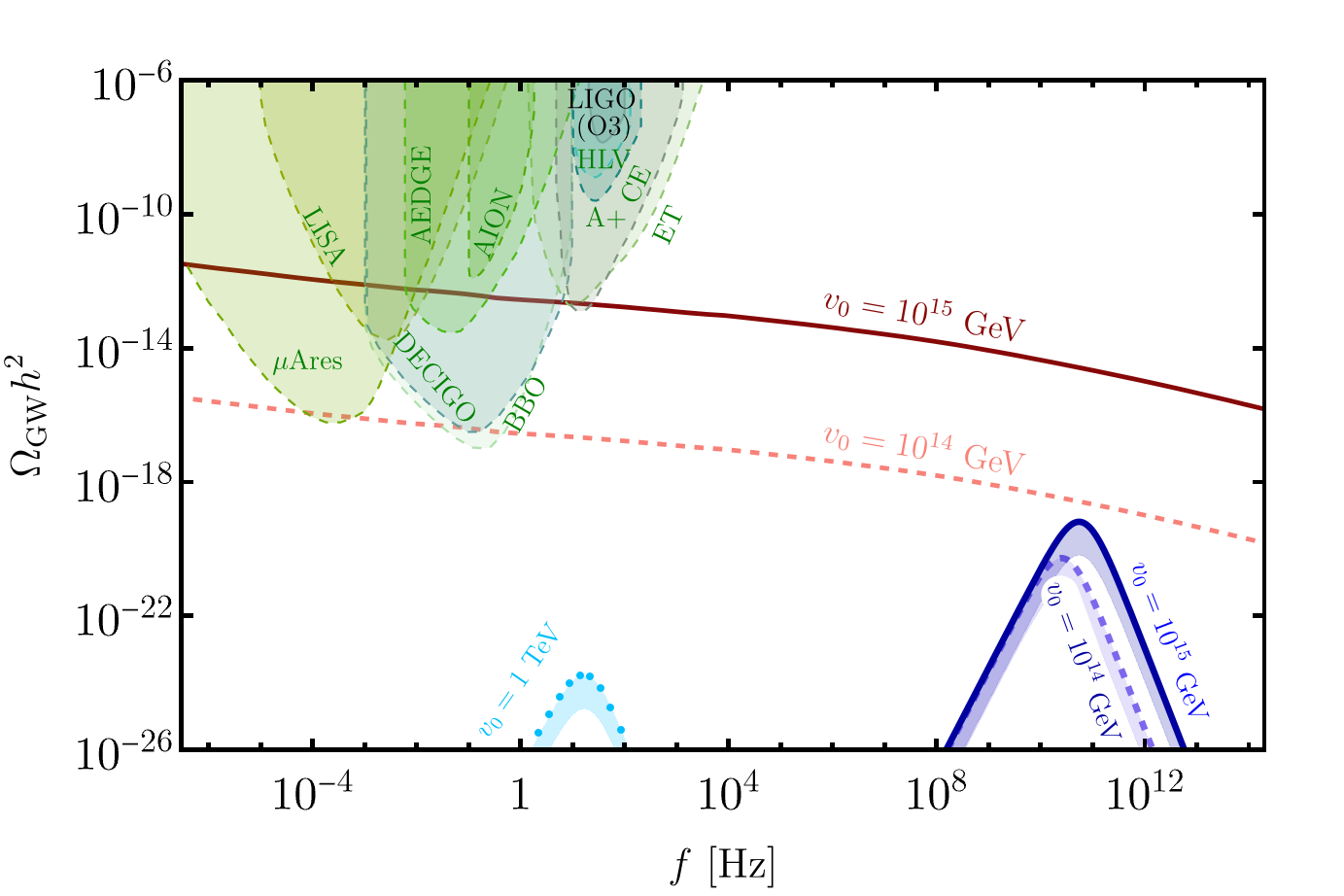
Figure 1: The blue bands denote the contribution to the predicted GW spectrum from first order phase transition for $v_{0}=10^{15}\,{\rm GeV}$ (solid line), $10^{14}\,{\rm GeV}$ (dashed line) and $1\,{\rm TeV}$ (dotted line). The red lines denote the contribution from cosmic strings for $v_{0}=10^{15}\,{\rm GeV}$ (solid line) and $10^{14}\,{\rm GeV}$ (dashed line), the signal for $v_{0}=1$ TeV is too suppressed to show here. The (green) shadowed regions show the sensitivity curves of the indicated experiments.

Considering that these three choices are those found in a scan that maximise the signal in respective peak frequencies, it should be clear that the contribution from phase transitions in the case of the minimal model is far below the experimental sensitivity. In this way we confirm the conclusions found in [19]. In the next subsection we point out, however, that at least for large values of $v_{0}$, the contribution from cosmic strings could be detectable in future experiments even in this minimal model.

Before concluding we should also mention that one could think to add an explicit symmetry breaking cubic term in the tree level potential. However, as noticed in [19], its coefficient is upper bounded by the observation that it unavoidably generates also a linear term in the effective potential. This tends to remove the barrier between the two vacua so that, if the coefficient is too large, there is no first order phase transition and, therefore, no GW production. For this reason, we do not pursue this scenario.

2.3 GW from global cosmic strings

Spontaneously breaking the $U(1)_{L}$ symmetry at high energies by the complex scalar $\phi$ generates a global cosmic string network, which dominantly radiates Goldstone bosons, and sub-dominantly emits gravitational waves [57]. Compared to the Nambu-Goto string-induced almost flat gravitational wave spectrum associated with a gauged symmetry breaking, the global cosmic string-induced gravitational waves are typically suppressed, and their amplitude mildly falls off with frequency for most of the spectrum of interest. This makes their detection at interferometers more challenging, unless the symmetry breaking scale $v_{0}$ is above $10^{14}$ GeV. In this section we briefly review the dynamics of global cosmic strings using the the velocity-dependent one scale (VOS) model [58, 59, 60, 61, 62, 63] and the associated gravitational wave spectrum following [64].

The global cosmic string network consists of horizon sized long strings that randomly intersect and form sub-horizon sized loops at the intersections. The network shrinks and loses energy with time, but eventually enters a scaling regime where the average inter-string separation scale $L$, and the ratio of the energy density of the network to the total background energy density remain constant. For Nambu-Goto strings, this energy is radiation from the string loops predominantly in the form of gravitational waves. However, for global strings the leading mode of energy radiation is from the emission of Goldstone particles, and only a fraction of the energy is radiated as gravitational waves.

The energy density of the global string network can be expressed as

$$\rho_{\rm cs}=\frac{\mu(t)}{L^{2}(t)}=\frac{\mu(t)}{t^{2}}\xi(t),$$ (47)

where $\mu(t)$ is the energy per unit length of the long strings, and $\xi(t)$ is a dimensionless parameter which represents the number of long strings per horizon volume. While for Nambu-Goto strings, $\mu$ is a constant, for global strings it has a logarithmic dependence on the ratio of two scales, a macroscopic scale $L(t)$ close to the Hubble scale, and a microscopic scale $\delta(t)\sim 1/(\lambda v_{0})$ representing the width of the string core,

$$\mu(t)=2\pi v_{0}^{2}\log{\frac{L(t)}{\delta}}\equiv 2\pi v_{0}^{2}N(t).$$ (48)

Here we have defined a dimensionless time parameter $N(t)\equiv\log[{L(t)/\delta(t)}]$. Eq. (48) can then be written as

$$N(t)+\frac{1}{2}\log{\xi(t)}=\log{v_{0}t},$$ (49)

assuming the quartic coupling $\lambda\sim 1$.

The evolution of the inter-string separation scale $L(t)$ and the average long string velocity $\bar{v}$ are given by a system of coupled differential equations,

$$\left(2-\frac{1}{N}\right)\frac{dL}{dt} =2HL\left(1+\bar{v}^{2}\right)+\frac{L\bar{v}^{2}}{\ell_{f}}+\bar{c}\bar{v}+s\frac{\bar{v}^{6}}{N},$$ (50)

$$\frac{d\bar{v}}{dt} =(1-\bar{v}^{2})\left(\frac{q}{L}-2H\bar{v}\right).$$ (51)

The first term on the RHS of Eq. (50) represents dilution effect from Hubble expansion. The second term gives a negligible thermal friction effect with a characteristic scale $\ell_{f}\propto\mu/T^{3}$. The third term stands for the loop chopping effect, where $\bar{c}$ is the rate of loop chopping. The fourth term represents the the backreaction due to the Goldstone emission. $\bar{q}$ is a momentum parameter. In analogy with Nambu-Goto strings, the solution of Eqs. (50) and (51) can be expressed as

$$L^{2}(t) =\frac{t^{2}}{8}\frac{n\bar{q}(\bar{q}+\bar{c})(1+\Delta)}{1-\frac{2}{n}-\frac{1}{2N(t)}},$$ (52)

$$\bar{v}^{2}(t) =\frac{1-\Delta}{2}\frac{n\bar{q}}{\bar{q}+\bar{c}}\left(1-\frac{2}{n}-\frac{1}{2N(t)}\right),$$ (53)

where $\Delta\equiv\bar{\kappa}/(N(\bar{q}+\bar{c}))$, $\bar{\kappa}\equiv s\bar{v}^{5}/(1-\Delta)^{5/2}$, and $n=3,4$ corresponds to matter and radiation domination, respectively. Fitting data extracted from the simulation results in Refs. [65, 66, 67], the VOS model parameters can be approximated as [64]

$$\{\bar{c},\bar{q},\bar{\kappa}\}\simeq\{0.497,0.284,5.827\}.$$ (54)

Since $\xi(t)=t^{2}/L^{2}(t)$ from Eq. (47), Eq. (52) can be used to express $\xi$ as a function of $N(t)$. Eq. (49) then expresses $N(t)$ as a function of $t$. Similarly, $\bar{v}$ can be expressed as function of $t$ from Eq. (53).

Assuming that the loop size during formation of the string network is given by $\ell_{i}\sim\alpha t_{i}$, and the fraction of energy density of the strings contributing to gravitational wave $F_{\alpha}\sim 0.1$ [68, 69], the formation rate of string loops is given by

$$\frac{d\rho_{0}}{dt}\times\mathcal{F}_{\alpha}=-\frac{d\rho_{\rm cs}}{dt}\times F_{\alpha}\times\mathcal{F}_{\alpha}=\mathcal{E}_{\rm loop}\frac{\mu}{t^{3}}F_{\alpha}\mathcal{F}_{\alpha},$$ (55)

where $\mathcal{F}_{\alpha}\sim 1$ is the loop size distribution function, and $\mathcal{E}_{\rm loop}\equiv\bar{c}\bar{v}\xi^{3/2}$ is the loop emission parameter.

After formation, the string loop rapidly oscillates and radiates energy in the form of Goldstone particles and gravitational waves until disappearing completely [57]

$$\frac{dE}{dt}=-\Gamma G\mu^{2}-\Gamma_{a}v_{0}^{2},$$ (56)

where we assume the benchmark values $\Gamma\sim 50$ [68, 70, 71, 72] and $\Gamma_{a}\sim 65$ [73, 74]. The size of a loop initial length $\ell_{i}=\alpha t_{i}$ at a later time can be expressed as

$$\ell(t)\simeq\alpha t_{i}-\Gamma G\mu(t-t_{i})-\frac{\Gamma_{a}}{2\pi}\frac{t-t_{i}}{\log{N}},$$ (57)

where the second and third terms represent the decrease in loop size for gravitational wave emission and Goldstone emission, respectively.

It is useful to decompose the radiation into a set of normal modes $\tilde{f}_{k}=2k/\tilde{\ell}$, where $k=1,2,3,\ldots$, and $\tilde{\ell}\equiv\ell(\tilde{t})$ is the instantaneous size of a loop when it radiates at $\tilde{t}$. Accordingly, the radiation parameters can be decomposed as $\Gamma=\sum_{k}\Gamma^{(k)}$ and $\Gamma_{a}=\sum_{k}\Gamma_{a}^{(k)}$, where

$$\Gamma^{(k)}=\frac{\Gamma k^{-4/3}}{\sum_{j=1}^{\infty}j^{-4/3}},\quad\text{and\quad}\Gamma_{a}^{(k)}=\frac{\Gamma_{a}k^{-4/3}}{\sum_{j=1}^{\infty}j^{-4/3}},$$ (58)

and the normalization factor is approximately $\sum_{j=1}^{\infty}j^{-4/3}\simeq 3.60$.

Taking redshift into account, the observed frequency at today’s interferometers is

$$f_{k}=\frac{a(\tilde{t})}{a(t_{0})}\tilde{f}_{k},$$ (59)

where $t_{0}$ is present time and the scale factor today is $a(t_{0})\equiv 1$. The relic gravitational wave amplitude is summed over all normal modes

$$\Omega_{\rm GW}(f)=\sum_{k}\Omega_{\rm GW}^{(k)}(f)=\sum\frac{1}{\rho_{c}}\frac{d\rho_{\rm GW}}{d\log{f_{k}}}.$$ (60)

From Eqs. (55) and (57), the contribution from an individual $k$ mode can be expressed as

$$\Omega_{\rm GW}^{(k)}(f)=\frac{\mathcal{F}_{a}F_{a}}{\alpha\rho_{c}}\frac{2k}{f}\int_{t_{f}}^{t_{0}}d\tilde{t}\frac{\mathcal{E}_{\rm loop}\left(t_{i}^{(k)}\right)}{t_{i}^{(k)4}}\frac{\Gamma^{(k)}G\mu^{2}}{\alpha+\Gamma G\mu+\frac{\Gamma_{a}}{2\pi N}}\left[\frac{a(\tilde{t})}{a(t_{0})}\right]^{5}\left[\frac{a\left(t_{i}^{(k)}\right)}{a(\tilde{t})}\right]^{3}\theta(\tilde{\ell})\theta(\tilde{t}-t_{i}),$$ (61)

where $t_{f}$ is the formation time of the string network. Heaviside theta functions ensure causality and energy conservation. $t_{i}^{(k)}$ represents the time when a loop is formed, which emits gravitational wave at the time $\tilde{t}$, and is given by

$$t_{i}^{(k)}=\frac{\tilde{\ell}(\tilde{t},f,k)+\left(\Gamma G\mu+\frac{\Gamma_{a}}{2\pi N}\right)\tilde{t}}{\alpha+\Gamma G\mu+\frac{\Gamma_{a}}{2\pi N}},$$ (62)

where the loop size can be written as $\tilde{\ell}=2ka(\tilde{t})/f$.

The frequency spectrum of the gravitational wave amplitude is calculated by numerically evaluating Eq. (61), and summing from $k=1$ to a large value to ensure convergence. Evidently, the spectrum can be divided into three regions. The first region corresponds to very high frequencies starting at $f_{v_{0}}$, where the signal falls off, and the exact shape depends on the initial conditions and very early stages of the string network evolution not fully captured by the VOS model. $f_{v_{0}}$ is related to the time when the Goldstone radiation becomes significant. In the intermediate radiation dominated region $f_{\rm eq}<f<f_{v_{0}}$, the spectrum gradually declines as $~{}\log^{3}{(1/f)}$. In the matter dominated region $f_{0}<f<f_{\rm eq}$, the spectrum behaves as $f^{-1/3}$. $f_{\rm eq}$ is related to the time of matter-radiation equality, and $f_{0}$ is related to the emission at the present time. These characteristic frequencies are given by

$$f_{v_{0}} \sim\frac{2}{\alpha t_{n}}\frac{a(t_{v_{0}})}{a(t_{0})}\sim 10^{10}\ \text{Hz},$$ (63)

$$f_{0} \sim\frac{2}{\alpha t_{0}}\sim 3.6\times 10^{-16}\ \text{Hz},$$ (64)

$$f_{\rm eq} \sim 1.8\times 10^{-7}\ \text{Hz}.$$ (65)

Although the gravitational wave spectrum from global cosmic strings span over a very wide frequency range, for our purposes we will be concerned mostly in the $\mu$-Hz to kilo-Hz range, where some of the planned interferometers are sensitive. This range falls under $f_{\rm eq}<f<f_{v_{0}}$. The gravitational wave spectrum can be approximately expressed in this regime by [64]

$$\Omega_{\mathrm{GW}}(f)h^{2}\simeq 8.8\times 10^{-18}\left(\dfrac{v_{0}}{10^{15}\mathrm{GeV}}\right)^{4}\log^{3}\left[\left(\dfrac{2}{\alpha f}\right)^{2}\dfrac{v_{0}}{t_{\mathrm{eq}}}\dfrac{1}{z_{\mathrm{eq}}^{2}\sqrt{\xi}}\Delta_{R}^{1/2}(f)\right]\Delta_{R}(f),$$ (66)

where $z_{\rm eq}\simeq 8000$ [75], and $\Delta_{R}(f)$ represents the effect of varying number of relativistic degrees of freedom over time:

$$\Delta_{R}(f)=\frac{g_{*}(f)}{g_{*}^{0}}\left(\frac{g_{*S}^{0}}{g_{*S}(f)}\right)^{4/3}.$$ (67)

There are several constraints on the global cosmic string formation scale $\sim v_{0}$. The dominant radiation mode from global strings is emission of Goldstone bosons. Assuming they remain massless, the upper limit on the total relic radiation energy density from CMB $\Delta N_{\rm eff}\lesssim 0.2$ [75] implies $v_{0}\lesssim 3.5\times 10^{15}$ GeV [64]. If we assume standard cosmology, non-observation of gravitational waves at Parkes Pulsar Timing Array (PPTA) [69, 76, 77] gives an upper bound $v_{0}<2\times 10^{15}$ GeV. Other constraints from inflation scale and CMB anisotropy bound require $v_{0}\lesssim\mathcal{O}(10^{15})$ GeV [78, 79]. Hence we consider the global lepton number symmetry violation at scales $\lesssim 10^{15}$ GeV. Furthermore, we require $T_{RH}\gtrsim v_{0}$ to ensure that the lepton number symmetry is restored in the early universe and symmetry breaking can take place at the scale $\sim v_{0}$.

We show the global cosmic string induced GW signals for $v_{0}=10^{14}$ and $10^{15}$ GeV in Fig. 1 with red curves. The former is within the sensitivity of upcoming interferometers $\mu$Ares, DECIGO and BBO, whereas the latter might be probed at LISA, AEDGE and Einstein Telescope as well. The phase transition signals for $v_{0}=10^{14}$ and $10^{15}$ GeV remain buried under their respective cosmic string signals. We therefore conclude that the single Majoron model can still be probed in GW interferometers through its cosmic string signal as long as the global lepton number symmetry is spontaneously broken in between $10^{14}$ and $10^{15}$ GeV.

3 GW from Majorana mass genesis in a two-Majoron model

As we discussed, the GW contribution to the stochastic background from a phase transition in the single Majoron model is by far below the sensitivity of planned experiments. The reason for the suppressed signal amplitude can be traced back to the fact that for a single scalar, the cubic term is strictly temperature dependent and vanishes at zero temperature. It was noticed in [19] that the signal can be strongly enhanced if an auxiliary scalar field is introduced. This would undergo its own phase transition getting its final VEV prior to the phase transition of the original scalar. In this way a bi-quadratic mixing term could be added to the tree level potential. This term generates a zero temperature barrier in the thermal effective potential able to enhance the strength of the phase transition $\alpha$ and, consequently, the GW spectrum. The nature of the auxiliary scalar field was not specified in [19]. Here we propose a model with two Majorons where the auxiliary scalar field is identified as a complex scalar field charged under a new global lepton number symmetry.

For definiteness, we call the complex scalars $\phi_{1}$, $\phi_{2}$, and their respective global lepton number symmetries $U(1)_{L_{1}}$, $U(1)_{L_{2}}$. The Lagrangian can be written as

$$-{\cal L}_{N_{I}+\phi_{i}} =\overline{L_{\alpha}}\,h_{\alpha I}\,N_{I}\,\widetilde{\Phi}+{y_{1}\over 2}\,\phi_{1}\,\overline{N_{1}^{c}}\,N_{1}+{y_{2}\over 2}\,\phi_{1}\,\overline{N_{2}^{c}}\,N_{2}+{y_{3}\over 2}\,\phi_{2}\,\overline{N_{3}^{c}}\,N_{3}+V_{0}(\phi_{1},\phi_{2})+{\rm h.c.}\,,$$ (68)

As before, we ignore any mixing between the SM Higgs doublet $\widetilde{\Phi}$ with the complex scalars $\phi_{1},\phi_{2}$. Here $\phi_{2}$ couples only to the RH neutrino $N_{3}$, whereas $\phi_{1}$ couples to both $N_{1}$ and $N_{2}$. This can be ensured by giving nonzero $U(1)_{L_{1}}$ charges to $N_{1}$ and $N_{2}$ and half of their complementary charge to $\phi_{1}$, whereas $N_{3}$ and $\phi_{2}$ have similar complementary charges under $U(1)_{L_{2}}$ only. Furthermore, we have chosen a basis where $\phi_{1}$ and $\phi_{2}$ only couple to the diagonal elements of the RH neutrino mass matrix.

As usual, we write the complex fields as $\phi_{1}=(\varphi_{1}+i\ \chi_{2})/\sqrt{2}$ and $\phi_{2}=(\varphi_{2}+i\ \chi_{2})/\sqrt{2}$ and assume that the vacuum expectation values are along the real axis, $\langle\phi_{1}\rangle=v_{1}/\sqrt{2}$ and $\langle\phi_{2}\rangle=v_{2}/\sqrt{2}$. After spontaneous breaking of both $U(1)$ symmetries, $\chi_{1}$ and $\chi_{2}$ are identified as two Majorons. We further assume the hierarchy $v_{2}\gg v_{1}$, so that the RH neutrino mass spectrum is hierarchical $M_{3}\gg M_{1},M_{2}$.

The $U(1)_{L_{1}}\times U(1)_{L_{2}}$ symmetry allows the usual quadratic and quartic terms for both $\phi_{1}$ and $\phi_{2}$. It also allows a quartic mixing between the two scalars, so that the tree level potential can now be written as

$$V_{0}(\phi_{1},\phi_{2})=-{\mu_{1}^{2}}|\phi_{1}|^{2}+\lambda_{1}|\phi_{1}|^{4}-{\mu_{2}^{2}}|\phi_{2}|^{2}+\lambda_{2}|\phi_{2}|^{4}+\zeta|\phi_{1}|^{2}|\phi_{2}|^{2}.$$ (69)

At sufficiently high temperatures, both symmetries are restored. At temperatures $T\sim v_{2}$, spontaneous breaking of $U(1)_{L_{2}}$ generates the massless Majoron field $\chi_{2}$. When the phase transition of $\phi_{2}$ has completed, the second phase transition of $\phi_{1}$ may start at around $T\sim v_{1}$. From this first phase transition we can expect a negligible contribution to the GW spectrum at observable frequencies, as we have seen in the previous section.

Let us now focus on the phase transition of $\phi_{1}$ at a lower scale. Writing the potential Eq. (69) in terms of the real fields $\varphi_{1}$, $\varphi_{2}$, and the minimization conditions yield

$$\mu_{1}^{2} =\lambda_{1}\,v_{1}^{2}+\frac{\zeta}{2}v_{2}^{2},$$ (70)

$$\mu_{2}^{2} =\lambda_{2}\,v_{2}^{2}+\frac{\zeta}{2}v_{1}^{2}.$$ (71)

Because of the mixing term in the potential, the scalar mass matrix has non-vanishing off-diagonal terms. Following [80], it can be diagonalized by rotating the basis vectors, so that $\varphi_{1}$ and $\varphi_{2}$ can be expressed in terms of the new mass eigenstates $\bar{\varphi}_{1}$ and $\bar{\varphi}_{2}$

$$\varphi_{1} =v_{1}+\bar{\varphi}_{1}\cos{\theta}-\bar{\varphi_{2}}\sin{\theta},$$ (72)

$$\varphi_{2} =v_{2}+\bar{\varphi}_{1}\sin{\theta}+\bar{\varphi_{2}}\cos{\theta},$$ (73)

where the rotation angle can be determined, assuming $v_{2}\gg v_{1}$, to be

$$\theta\simeq-\frac{\zeta v_{1}}{2\lambda_{2}v_{2}}.$$ (74)

In this basis, expanding the quartic mixing term in Eq. (69) in terms of the mass eigenstates yields a cubic term for $\bar{\varphi}_{1}$,

$$\frac{\zeta}{4}\varphi_{1}^{2}\varphi_{2}^{2} \xrightarrow{v_{2}\gg v_{1}}-\frac{\zeta^{2}}{2}\frac{v_{2}}{\lambda_{2}}\bar{\varphi}_{1}^{3}+\ldots$$ (75)

Since the mixing angle $\theta$ is very small, the mass eigenstate $\bar{\varphi}_{1}$ almost coincides with $\varphi_{1}$. Hence the net effect is the appearance of a new cubic term in the thermal effective potential of $\varphi_{1}$,

$$V_{\rm eff}(\varphi_{1},T)\approx{1\over 2}\,\widetilde{M}_{T}^{2}\,\varphi_{1}^{2}-(A\,T+C)\,\varphi_{1}^{3}+\frac{1}{4}\lambda_{T}\,\varphi_{1}^{4}\,,$$ (76)

where $C={\zeta^{2}v_{2}}/({2}{\lambda_{2}})$. Comparing Eq. (76) to Eq. (19), the expressions for $\widetilde{M}_{T},A$ and $\lambda_{T}$ are obtained from Eqs. (20)-(23) with the replacement $\lambda\rightarrow\lambda_{1},v_{0}\rightarrow v_{1}$. Since the heaviest RH neutrino mass $M_{3}\sim v_{2}\gg v_{1}$, we can assume that the $N_{3}$’s have fully decayed at the onset of the $\phi_{1}$ phase transition. On the other hand, we can assume that both the lighter RH neutrinos are fully thermalised and, therefore, take $N=2$.

The cubic term at zero temperature helps to strengthen the phase transition of $\phi_{1}$. To illustrate this, we perform a random scan over the model parameters $(\lambda_{1},v_{1},C)$ in the range $10^{-6}\leq\lambda_{1}\leq 1$, $1\leq v_{1}/\text{GeV}\leq 10^{7}$, $10^{-4}\leq M/v_{1}\leq 10$ and $10^{-8}\leq C/v_{1}\leq 1$ and calculate the GW parameters $T_{\star}$, $\alpha$ and $\beta/H_{\star}$, following section 2.2. In Fig. 2 we show the results of the scan, where the color map represents $\log_{10}T_{\star}/{\rm GeV}$ at each point. The model allows $\alpha\gtrsim\mathcal{O}(1)$ and $\beta\gtrsim 10^{7}$, however, as we discussed, we consider only points for $\alpha\leq 0.3$ and $\beta/H_{\star}>100$.

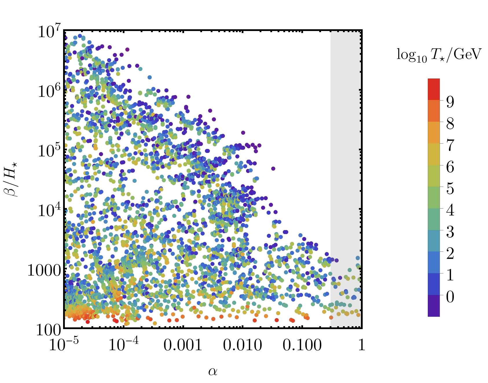
Figure 2: GW parameters $\alpha$ and $\beta/H_{\star}$ from scan over the model parameters $\lambda_{1}$, $v_{1}$, $M$ and $C$. The color bar represents $\log_{10}T_{\star}/{\rm GeV}$ for each point.

To get a better understanding of how $T_{\star}$, $\alpha$ and $\beta/H_{\star}$ depend on the model parameters, we look at a two-dimensional slice of the parameter space in terms of $\{\lambda_{1},v_{1}\}$ setting $M=0.15v_{1}$ and $C=0.002v_{1}$. The results are shown in Fig. 3. We find that $T_{\star}\sim\mathcal{O}(v_{1})$ and is nearly independent of $\lambda_{1}$. On the other hand $\alpha$ is essentially determined by $\lambda_{1}$, and peaks near $\lambda_{1}\sim\mathcal{O}(10^{-4})$. Finally, $\beta/H_{\star}$ depends on both $\lambda_{1}$ and $v_{1}$.

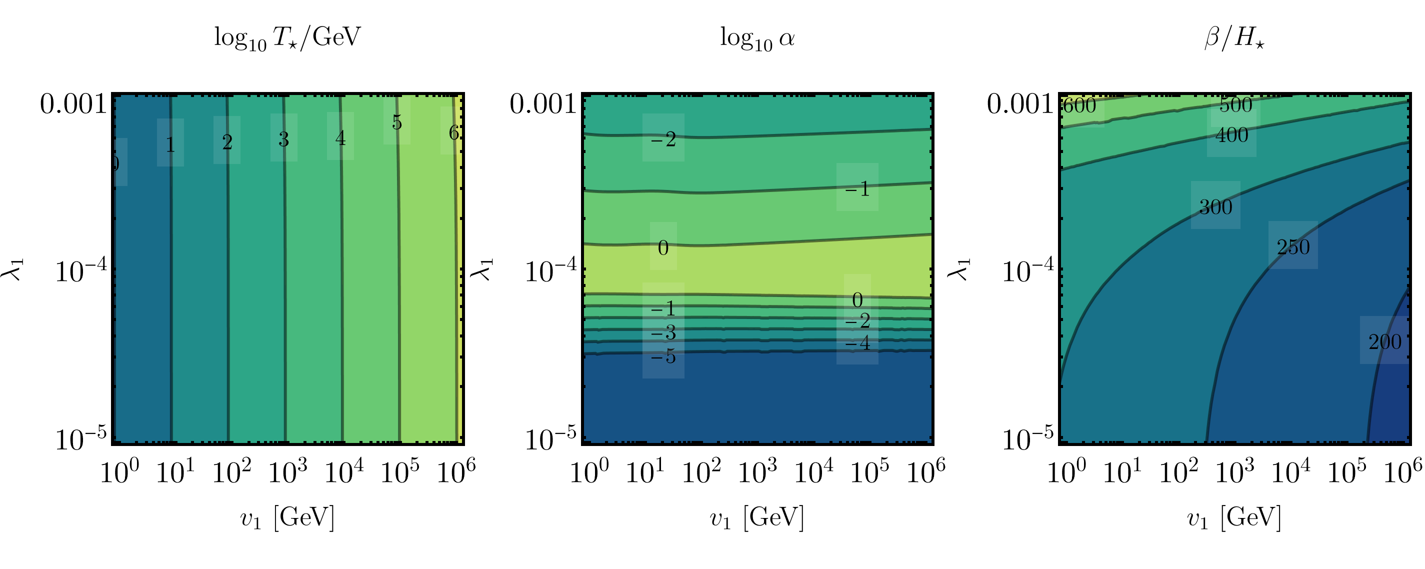
Figure 3: Dependence of the GW parameters $T_{\star}$, $\alpha$ and $\beta/H_{\star}$ on the model parameters $\lambda_{1}$ and $v_{1}$, setting $M=0.15v_{1}$ and $C=0.002v_{1}$.

We now look at the gravitational wave spectrum for the three benchmark points listed in Table 2. The benchmark points have been chosen to maximize the GW amplitude from first order phase transition in their respective peak frequencies. The resulting signals are shown in Fig. 4, along with the GW spectrum from the global cosmic strings for $v_{2}=10^{15}$, $5\times 10^{14}$, $2\times 10^{14}$ and $10^{14}$ GeV. The peak amplitude of these signals are consistent with what one would expect from the range of $\alpha$ and $\beta/H_{\star}$ where our calculation of GW spectrum is valid, as discussed in Appendix A.

B.P.	$\lambda_{1}$	$v_{1}$ [GeV]	$M$ [GeV]	$C$ [GeV]	$\alpha$	$\beta/H_{\star}$	$T_{\star}$ [GeV]	$\langle\varphi_{1}\rangle^{\rm true}_{T_{\star}}$ [GeV]
	$0.00057$	$1188.22$	$186.53$	$20.79$	$0.29$	$244.65$	$5863.12$	$1.38\times 10^{5}$
	$0.00061$	$2.32\times 10^{5}$	$3.63\times 10^{4}$	$3023.02$	$0.30$	$204.66$	$7.81\times 10^{5}$	$1.79\times 10^{7}$
	$0.00036$	$9.88\times 10^{6}$	$1.08\times 10^{6}$	$2\times 10^{6}$	$0.30$	$141.48$	$7.51\times 10^{8}$	$1.92\times 10^{10}$

Table 2: Benchmark points for gravitational wave signals from first order phase transition of $\varphi_{1}$.

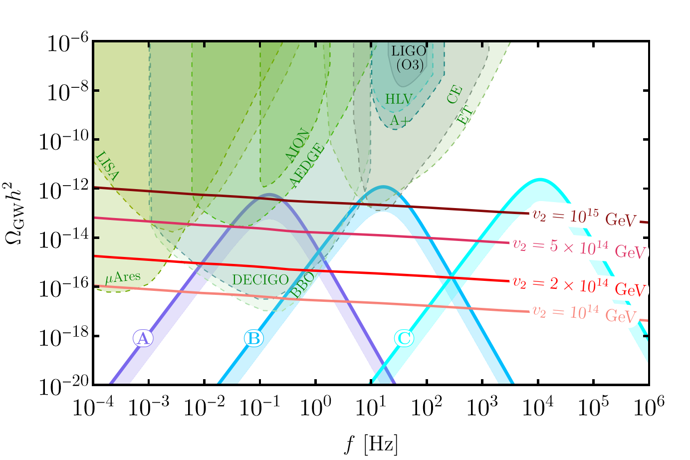
Figure 4: Gravitational wave spectrum from first order phase transition of $v_{1}$ for three benchmark points shown in Table 2 and from global cosmic string formed by spontaneous breaking of the global $U(1)_{L_{2}}$ symmetry by $\phi_{2}$ for four representative cases. The shaded region in the phase transition signals represent uncertainties in the calculation of the gravitational wave amplitude. Sensitivities and upper bounds from various upcoming and present interferometers are also shown.

The peak amplitude of the benchmark points and are sensitive to DECIGO, BBO, AEDGE, and ET, CE, respectively, while point peaks at a higher frequency. In all cases, the peak amplitude is larger than the global cosmic string induced spectrum for $v_{2}\lesssim 10^{15}$ GeV. For any benchmark point and a given $v_{2}$, the combined gravitational wave spectrum would look like a peak towering above the slightly tilted plateau. While the wideband nature of the global cosmic string induced signal offers detection possibility at multiple interferometers, the larger peak from first order phase transition provides better visibility. Combining the two features, a unique gravitational wave signal emerges for models with two scalars, one breaking a global $U(1)$ symmetry at ultraviolet scales and the other undergoing a strong first order phase transition at lower scales.

4 GW from Majorana mass genesis in a three-Majoron model

A straightforward generalization of the model is to include three complex scalars with hierarchical VEVs, so that each scalar gives mass to one of the RH neutrinos,

$$-\mathcal{L}_{N_{I}+\phi_{I}} \supset h_{aI}\bar{L}_{a}HN_{I}+\frac{1}{2}y_{1}\phi_{1}\overline{N^{c}_{1}}N_{1}+\frac{1}{2}y_{2}\phi_{2}\overline{N^{c}_{2}}N_{2}+\frac{1}{2}y_{3}\phi_{3}\overline{N^{c}_{3}}N_{3}+V_{0}(\phi_{1},\phi_{2},\phi_{3})$$

$$+\text{h.c.}.$$ (77)

The Lagrangian has a $U(1)_{L_{1}}\times U(1)_{L_{2}}\times U(1)_{L_{3}}$ symmetry, with each $U(1)$ corresponding to each scalar. We denote the VEVs as $\langle\phi_{I}\rangle\equiv v_{I}$ and without loss of generality assume $v_{3}\gg v_{2}\gg v_{1}$. The tree-level scalar potential is given by

$$V_{0}(\phi_{1},\phi_{2},\phi_{3}) =\sum_{I=1,2,3}\left[-\mu_{I}^{2}\phi_{I}^{*}\phi_{I}+\lambda_{I}(\phi_{I}^{*}\phi_{I})^{2}\right]+\sum_{I,J,I\neq J}^{1,2,3}\frac{\zeta_{IJ}}{2}(\phi_{I}^{*}\phi_{I})(\phi_{J}^{*}\phi_{J}).$$ (78)

After spontaneous breaking of the global lepton number symmetries, the three RH neutrinos get nonzero Majorana mass from the VEV of $\phi_{1}$, $\phi_{2}$, $\phi_{3}$. Assuming these VEVs are along the real axis, one can identify the imaginary part of the complex scalars as massless Majorons.

The mixing terms $\zeta_{IJ}$ in Eq. (78) introduce a zero temperature cubic term to the effective potential of a scalar with smaller VEV. As before, the phase transition of $\phi_{3}$ occurring at around the scale $v_{3}$ is not expected to generate any strong gravitational wave signal, since there is no zero temperature cubic term in its effective potential. However, the spontaneous breaking of $U(1)_{L_{3}}$ at this scale would generate global cosmic string induced gravitational waves, which can be probed if $v_{3}\gtrsim 10^{14}$ GeV. Suppose the phase transition of $\phi_{3}$ is completed before the universe cools down to the scale $v_{2}$, when $\phi_{2}$ undergoes a phase transition. The quartic mixing of $\phi_{2}$ with $\phi_{3}$ now introduces a zero temperature cubic term to the thermal effective potential of $\phi_{2}$, resulting in a strong first order phase transition and associated gravitational wave from the sound waves. At this stage $\phi_{1}$ does not play any role in the phase transition of $\phi_{2}$. Then, during the phase transition of $\phi_{1}$ at around the scale $v_{1}$, the other two scalars have already completed their phase transition and together they would introduce an effective zero temperature cubic term from their mixing with $\phi_{1}$, resulting in a strong phase transition and subsequent gravitational wave signal.

	$\lambda_{I}$	$v_{I}$ [GeV]	$M_{I}$ [GeV]	$C_{I}$ [GeV]	$\alpha$	$\beta/H_{\star}$	$T_{\star}$ [GeV]	$\langle\varphi_{I}\rangle^{\rm true}_{T_{\star}}$ [GeV]
	$0.00027$	$1188.2$	$186.5$	$10.79$	$0.30$	$241.37$	$5196.52$	$1.50\times 10^{5}$
	$0.00029$	$2.32\times 10^{5}$	$3.63\times 10^{4}$	$1523.02$	$0.30$	$203.53$	$6.7\times 10^{5}$	$1.88\times 10^{7}$

Table 3: Benchmark point for gravitational wave signal from first order phase transition of $\varphi_{1}$, denoted by ($I=1$) and $\varphi_{2}$, denoted by ($I=2$).

Typically the percolation temperature $T_{\star}$ is proportional to the VEV of the corresponding scalar undergoing the phase transition. From Eq. (39), this implies that the combined effect of the phase transition of the three scalars may yield a double peaked gravitational wave spectrum, with one peak at a lower frequency due to the phase transition of $\phi_{1}$, and another peak at a higher frequency due to the phase transition of $\phi_{2}$. Together with a global cosmic string induced gravitational wave spectrum from $U(1)_{L_{3}}$ breaking, the combined amplitude of the gravitational wave signal may resemble twin peaks over a slightly slanted plateau, if the phase transition signals are sufficiently strong. In Table 3, we show a benchmark point consisting of the phase transition of $\phi_{1}$, denoted by and the phase transition of $\phi_{2}$, denoted by , that together with $v_{3}=2\times 10^{14}$ GeV generate the combined gravitational wave signal shown in Fig. 5. Notice that in this case we have assumed that at each phase transition $N=1$, corresponding to a situation where only the RH neutrino species $N_{I}$, coupling to its associated scalar field $\phi_{I}$ undergoing the phase transition, is fully thermalised, while the other two either have fully decayed or have not yet thermalised. This assumption is quite natural because of the strong hierarchy we are assuming for the $v_{I}$’s, implying that a strong hierarchy of the RH neutrino mass spectrum and in turn of the equilibration temperatures (see Eq. (13).

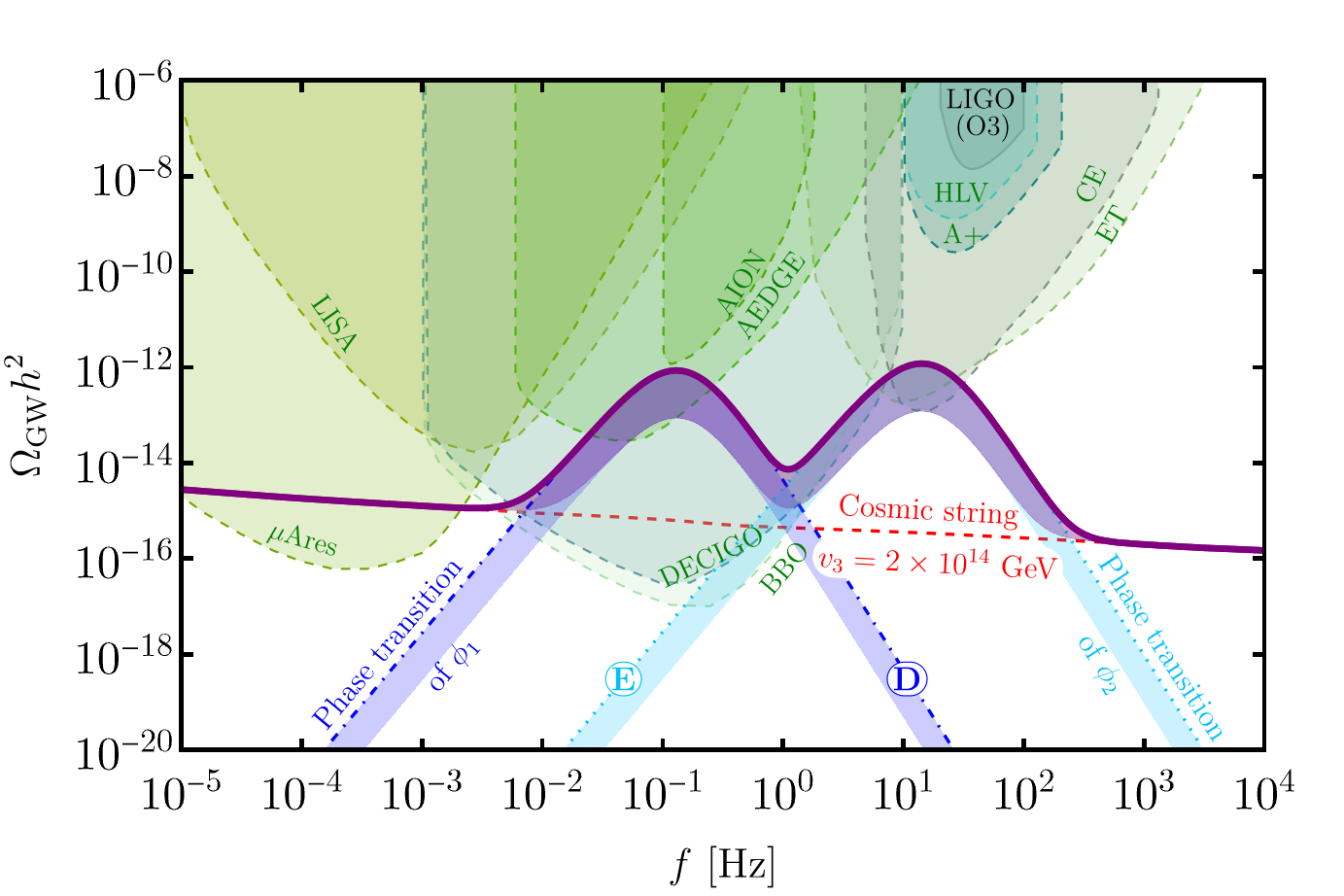
Figure 5: Gravitational wave spectrum from first order phase transition of $\phi_{1}$ and $\phi_{2}$, with corresponding parameters shown in rows and , respectively, in Table 3, and from cosmic string formed by spontaneous breaking of the global $U(1)_{L_{3}}$ symmetry by $\phi_{3}$ at $v_{3}=2\times 10^{14}$ GeV. Individual GW contributions are shown with dotted, dashed and dotdashed lines, while the combined spectrum is shown with a solid curve. Band in GW spectrum from phase transition represent the possible $\mathcal{O}(0.1)$ suppression in the parameter $\widetilde{\Omega}_{\rm gw}$.

5 Conclusion

We have investigated the gravitational wave signatures of the Majoron model of neutrino mass generation and have identified two sources of gravitational waves. In the simplest single Majoron model, a complex scalar couples to the RH neutrinos and generates their Majorana mass after spontaneously breaking the global lepton number symmetry. The breaking of a global symmetry creates global cosmic strings which can produce gravitational waves, with a different spectrum as compared to that from local Nambu-Goto strings. In the observable frequency window, the amplitude of this signal mildly declines as $\log^{3}[{1/f}]$, and still remains sensitive to upcoming GW interferometers if the symmetry is broken at a scale in between $10^{14}-10^{15}$ GeV. However, there is a possible additional source of GWs in this model, since the complex scalar gets a nonzero vacuum expectation value and in the process might undergo a first order phase transition. If such a phase transition is sufficiently strong, it could generate a peaked GW signal which may tower over the global cosmic string signal.

For the simplest model with just one complex scalar coupling to all three RH neutrinos, we confirm the result of Ref. [19] that the phase transition signal is too feeble to be detected. However, we point out that the global cosmic string signal even in this model can be detected if the lepton number symmetry is broken at around $10^{14}-10^{15}$ GeV.

We then considered an extended Majoron model, introducing two complex scalars with hierarchical vacuum expectation values, one giving mass to the heaviest RH neutrino and the other to the remaining two lighter ones. Assuming the scalars are charged under separate lepton number symmetries and have a quartic mixing between them, we explored the global cosmic string induced GW spectrum which is generated when the heaviest RH neutrino gets a mass. We showed that, while the phase transition of the associated scalar remains weak, its mixing with the other scalar introduces a zero-temperature cubic term to the potential of the latter, and greatly enhances the GW signal from its phase transition. We have discussed examples where the combined GW spectrum of the model may have an observable bump or peak due to the phase transition signal, visible in the slanted plateau region from the cosmic string signal, where such a bump may appear anywhere over the whole range of observable frequencies.

Finally, we have discussed an interesting possibility of a double peaked spectrum which may occur over the global cosmic string plateau region, where such a spectrum may arise from an extension of the Majoron model to include three complex scalars. This rather plausible model is easily implemented for a hierarchical RH neutrino mass spectrum, where each RH Neutrino gets its mass from the spontaneous breaking of its respective lepton number symmetry. Such a double peaked spectrum provides a characteristic signature of the three Majoron model of neutrino mass generation.

We have also noticed how the observation of such a GW spectrum would give us a precious information on the cosmological history and in particular on the reheating temperature of the universe. We have implicitly assumed that this was higher than all vacuum expectation values and critical temperatures so that the GW spectra are produced through the entire range of corresponding frequencies. However, if the reheating temperature is below the vacuum expectation value of one of the complex scalar fields, then the phase transition would not take place and the signal would be absent. At the same time it should be mentioned that the model we have presented can be clearly combined with (minimal) leptogenesis [15] since the decays of the RH neutrinos would produce a $B-L$ asymmetry that can then be partly converted into a baryon asymmetry. Therefore, the observation of the GW spectra in this model would also provide a strong test of leptogenesis. Moreover, as proposed in [81], a phase transition of the complex scalar field can be also associated to the production of a dark RH neutrino playing the role of dark matter [82]. Future GW experiments have then the potential to shed light on neutrino mass genesis, cosmological history and origin of matter of the universe.

Appendix A Dependence of peak GW amplitude on FOPT parameters

The peak of the GW amplitude from sound waves can be expressed as a function of FOPT parameters $\alpha$ and $\beta/H_{\star}$, as seen from Eq. (35). In Fig. 6 we show contours of $\log_{10}{\Omega_{\rm sw0}^{\rm peak}h^{2}}$. This plot shows that typically the peak amplitude of GW sourced by sound waves would be weaker than $10^{-11}$, as we have seen in the benchmark points of Figs. 4 and 5.

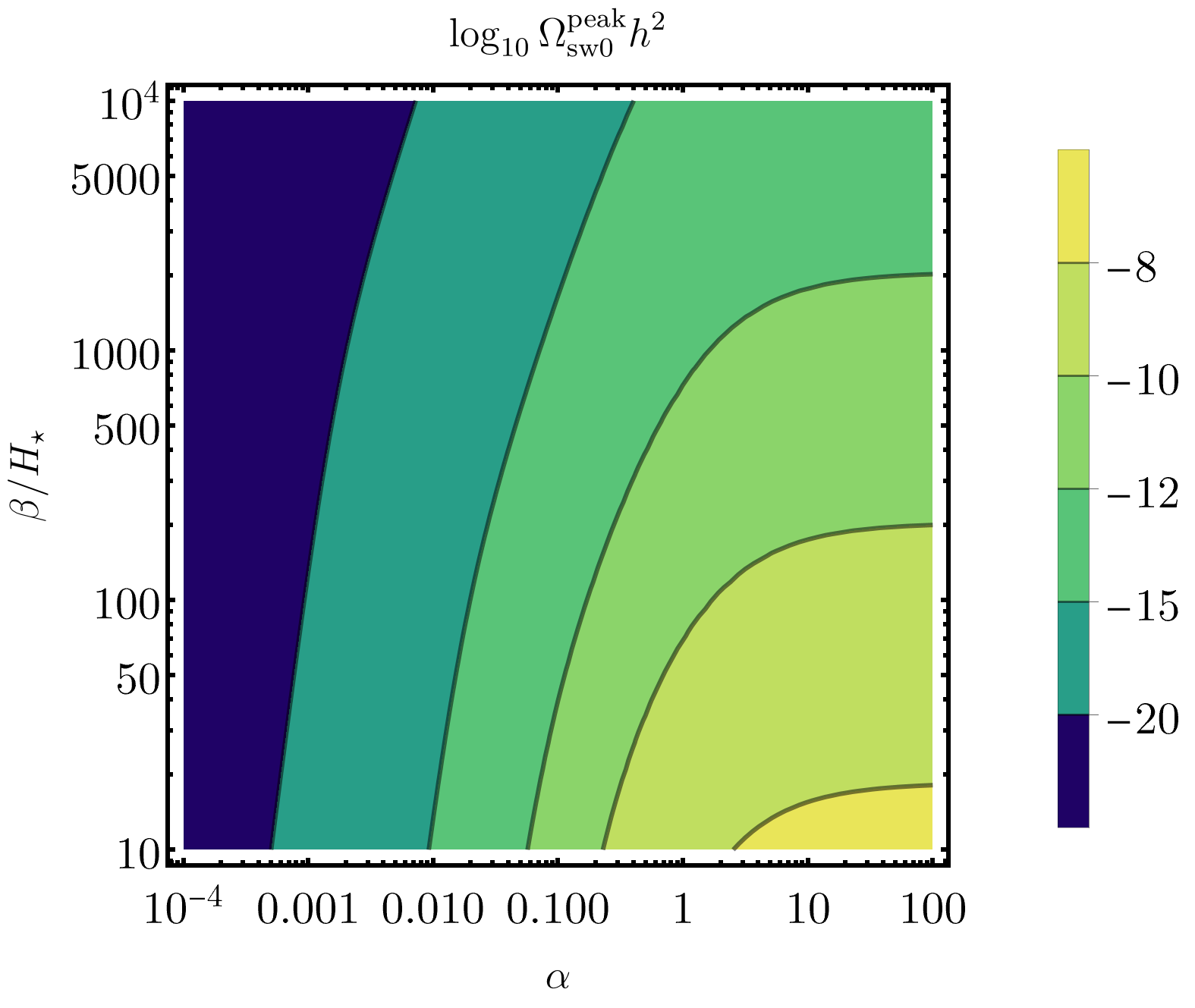
Figure 6: Contours of the peak GW amplitude from sound waves as a function of $\alpha$ and $\beta/H_{\star}$.

References

- [1] LIGO Scientific, Virgo collaboration, Observation of Gravitational Waves from a Binary Black Hole Merger, Phys. Rev. Lett. 116 (2016) 061102 [1602.03837].
- [2] A. Vilenkin, Cosmic Strings and Domain Walls, Phys. Rept. 121 (1985) 263.
- [3] E. Witten, Cosmic Separation of Phases, Phys. Rev. D 30 (1984) 272.
- [4] C.J. Hogan, Gravitational radiation from cosmological phase transitions, Mon. Not. Roy. Astron. Soc. 218 (1986) 629.
- [5] M.S. Turner and F. Wilczek, Relic gravitational waves and extended inflation, Phys. Rev. Lett. 65 (1990) 3080.
- [6] B. Fu and S.F. King, Gravitational wave signals from leptoquark-induced first-order electroweak phase transitions, JCAP 05 (2023) 055 [2209.14605].
- [7] S.F. King, S. Pascoli, J. Turner and Y.-L. Zhou, Confronting SO(10) GUTs with proton decay and gravitational waves, JHEP 10 (2021) 225 [2106.15634].
- [8] S.F. King, S. Pascoli, J. Turner and Y.-L. Zhou, Gravitational Waves and Proton Decay: Complementary Windows into Grand Unified Theories, Phys. Rev. Lett. 126 (2021) 021802 [2005.13549].
- [9] Y. Chikashige, R.N. Mohapatra and R.D. Peccei, Are There Real Goldstone Bosons Associated with Broken Lepton Number?, Phys. Lett. B 98 (1981) 265.
- [10] P. Minkowski, at a Rate of One Out of Muon Decays?, Phys. Lett. B 67 (1977) 421.
- [11] T. Yanagida, Horizontal gauge symmetry and masses of neutrinos, Proceedings of the Workshop on Unified Theory and Baryon Number of the Universe, (1979) .
- [12] M. Gell-Mann, P. Ramond and R. Slansky, in Sanibel talk, retroprinted as [9809459], and in Supergravity, North-Holland, Amsterdam (1979), PRINT-80-0576, retroprinted as [1306.4669], .
- [13] S. Glashow, The Future of Elementary Particle Physics, NATO Sci. Ser. B 61 (1980) 687.
- [14] R.N. Mohapatra and G. Senjanovic, Neutrino Mass and Spontaneous Parity Nonconservation, Phys. Rev. Lett. 44 (1980) 912.
- [15] M. Fukugita and T. Yanagida, Baryogenesis Without Grand Unification, Phys. Lett. B 174 (1986) 45.
- [16] A. Addazi, A. Marcianò, A.P. Morais, R. Pasechnik, R. Srivastava and J.W.F. Valle, Gravitational footprints of massive neutrinos and lepton number breaking, Phys. Lett. B 807 (2020) 135577 [1909.09740].
- [17] A. Addazi, Y.-F. Cai, Q. Gan, A. Marciano and K. Zeng, NANOGrav results and dark first order phase transitions, Sci. China Phys. Mech. Astron. 64 (2021) 290411 [2009.10327].
- [18] NANOGrav collaboration, The NANOGrav 12.5 yr Data Set: Search for an Isotropic Stochastic Gravitational-wave Background, Astrophys. J. Lett. 905 (2020) L34 [2009.04496].
- [19] P. Di Bari, D. Marfatia and Y.-L. Zhou, Gravitational waves from first-order phase transitions in Majoron models of neutrino mass, JHEP 10 (2021) 193 [2106.00025].
- [20] A. Sesana et al., Unveiling the gravitational universe at -Hz frequencies, Exper. Astron. 51 (2021) 1333 [1908.11391].
- [21] DECIGO working group collaboration, Primordial gravitational wave and DECIGO, PoS KMI2019 (2019) 019.
- [22] AEDGE collaboration, AEDGE: Atomic Experiment for Dark Matter and Gravity Exploration in Space, EPJ Quant. Technol. 7 (2020) 6 [1908.00802].
- [23] L. Badurina et al., AION: An Atom Interferometer Observatory and Network, JCAP 05 (2020) 011 [1911.11755].
- [24] C. Caprini et al., Science with the space-based interferometer eLISA. II: Gravitational waves from cosmological phase transitions, JCAP 04 (2016) 001 [1512.06239].
- [25] S. Hild et al., Sensitivity Studies for Third-Generation Gravitational Wave Observatories, Class. Quant. Grav. 28 (2011) 094013 [1012.0908].
- [26] K. Yagi and N. Seto, Detector configuration of DECIGO/BBO and identification of cosmological neutron-star binaries, Phys. Rev. D 83 (2011) 044011 [1101.3940].
- [27] LIGO Scientific collaboration, Exploring the Sensitivity of Next Generation Gravitational Wave Detectors, Class. Quant. Grav. 34 (2017) 044001 [1607.08697].
- [28] W. Buchmüller, V. Domcke, K. Kamada and K. Schmitz, The Gravitational Wave Spectrum from Cosmological Breaking, JCAP 10 (2013) 003 [1305.3392].
- [29] J.A. Dror, T. Hiramatsu, K. Kohri, H. Murayama and G. White, Testing the Seesaw Mechanism and Leptogenesis with Gravitational Waves, Phys. Rev. Lett. 124 (2020) 041804 [1908.03227].
- [30] B. Fornal and B. Shams Es Haghi, Baryon and Lepton Number Violation from Gravitational Waves, Phys. Rev. D 102 (2020) 115037 [2008.05111].
- [31] J. Bosch, Z. Delgado, B. Fornal and A. Leon, Gravitational Wave Signatures of Gauged Baryon and Lepton Number, 2306.00332.
- [32] D.A. Kirzhnits and A.D. Linde, Macroscopic Consequences of the Weinberg Model, Phys. Lett. B 42 (1972) 471.
- [33] L. Dolan and R. Jackiw, Symmetry Behavior at Finite Temperature, Phys. Rev. D 9 (1974) 3320.
- [34] G.W. Anderson and L.J. Hall, The Electroweak phase transition and baryogenesis, Phys. Rev. D 45 (1992) 2685.
- [35] M. Dine, R.G. Leigh, P.Y. Huet, A.D. Linde and D.A. Linde, Towards the theory of the electroweak phase transition, Phys. Rev. D 46 (1992) 550 [hep-ph/9203203].
- [36] M. Quiros, Finite temperature field theory and phase transitions, in ICTP Summer School in High-Energy Physics and Cosmology, pp. 187–259, 1, 1999 [hep-ph/9901312].
- [37] B. Garbrecht, F. Glowna and P. Schwaller, Scattering Rates For Leptogenesis: Damping of Lepton Flavour Coherence and Production of Singlet Neutrinos, Nucl. Phys. B 877 (2013) 1 [1303.5498].
- [38] P. Di Bari, K. Farrag, R. Samanta and Y.L. Zhou, Density matrix calculation of the dark matter abundance in the Higgs induced right-handed neutrino mixing model, JCAP 10 (2020) 029 [1908.00521].
- [39] R.R. Parwani, Resummation in a hot scalar field theory, Phys. Rev. D 45 (1992) 4695 [hep-ph/9204216].
- [40] D. Curtin, P. Meade and H. Ramani, Thermal Resummation and Phase Transitions, Eur. Phys. J. C 78 (2018) 787 [1612.00466].
- [41] D. Croon, O. Gould, P. Schicho, T.V.I. Tenkanen and G. White, Theoretical uncertainties for cosmological first-order phase transitions, JHEP 04 (2021) 055 [2009.10080].
- [42] S.R. Coleman, The Fate of the False Vacuum. 1. Semiclassical Theory, Phys. Rev. D 15 (1977) 2929.
- [43] A.D. Linde, Decay of the False Vacuum at Finite Temperature, Nucl. Phys. B 216 (1983) 421.
- [44] A.H. Guth and S.H.H. Tye, Phase Transitions and Magnetic Monopole Production in the Very Early Universe, Phys. Rev. Lett. 44 (1980) 631.
- [45] A.H. Guth and E.J. Weinberg, Cosmological Consequences of a First Order Phase Transition in the SU(5) Grand Unified Model, Phys. Rev. D 23 (1981) 876.
- [46] A. Megevand and S. Ramirez, Bubble nucleation and growth in very strong cosmological phase transitions, Nucl. Phys. B 919 (2017) 74 [1611.05853].
- [47] J. Ellis, M. Lewicki and J.M. No, Gravitational waves from first-order cosmological phase transitions: lifetime of the sound wave source, JCAP 07 (2020) 050 [2003.07360].
- [48] M. Hindmarsh, S.J. Huber, K. Rummukainen and D.J. Weir, Shape of the acoustic gravitational wave power spectrum from a first order phase transition, Phys. Rev. D 96 (2017) 103520 [1704.05871].
- [49] D. Cutting, M. Hindmarsh and D.J. Weir, Vorticity, kinetic energy, and suppressed gravitational wave production in strong first order phase transitions, Phys. Rev. Lett. 125 (2020) 021302 [1906.00480].
- [50] M. Kamionkowski, A. Kosowsky and M.S. Turner, Gravitational radiation from first order phase transitions, Phys. Rev. D 49 (1994) 2837 [astro-ph/9310044].
- [51] P.J. Steinhardt, Relativistic Detonation Waves and Bubble Growth in False Vacuum Decay, Phys. Rev. D 25 (1982) 2074.
- [52] J.R. Espinosa, T. Konstandin, J.M. No and G. Servant, Energy Budget of Cosmological First-order Phase Transitions, JCAP 06 (2010) 028 [1004.4187].
- [53] J. Ellis, M. Lewicki and J.M. No, On the Maximal Strength of a First-Order Electroweak Phase Transition and its Gravitational Wave Signal, JCAP 04 (2019) 003 [1809.08242].
- [54] H.-K. Guo, K. Sinha, D. Vagie and G. White, Phase Transitions in an Expanding Universe: Stochastic Gravitational Waves in Standard and Non-Standard Histories, JCAP 01 (2021) 001 [2007.08537].
- [55] KAGRA, LIGO Scientific, Virgo, VIRGO collaboration, Prospects for observing and localizing gravitational-wave transients with Advanced LIGO, Advanced Virgo and KAGRA, Living Rev. Rel. 21 (2018) 3 [1304.0670].
- [56] KAGRA, Virgo, LIGO Scientific collaboration, Upper limits on the isotropic gravitational-wave background from Advanced LIGO and Advanced Virgo’s third observing run, Phys. Rev. D 104 (2021) 022004 [2101.12130].
- [57] A. Vilenkin and T. Vachaspati, Radiation of Goldstone Bosons From Cosmic Strings, Phys. Rev. D 35 (1987) 1138.
- [58] C.J.A.P. Martins and E.P.S. Shellard, Quantitative string evolution, Phys. Rev. D 54 (1996) 2535 [hep-ph/9602271].
- [59] C.J.A.P. Martins and E.P.S. Shellard, Extending the velocity dependent one scale string evolution model, Phys. Rev. D 65 (2002) 043514 [hep-ph/0003298].
- [60] C.J.A.P. Martins, J.N. Moore and E.P.S. Shellard, A Unified model for vortex string network evolution, Phys. Rev. Lett. 92 (2004) 251601 [hep-ph/0310255].
- [61] C.J.A.P. Martins and M.M.P.V.P. Cabral, Physical and invariant models for defect network evolution, Phys. Rev. D 93 (2016) 043542 [1602.08083].
- [62] C.J.A.P. Martins, Scaling properties of cosmological axion strings, Phys. Lett. B 788 (2019) 147 [1811.12678].
- [63] J.R.C.C.C. Correia and C.J.A.P. Martins, Extending and Calibrating the Velocity dependent One-Scale model for Cosmic Strings with One Thousand Field Theory Simulations, Phys. Rev. D 100 (2019) 103517 [1911.03163].
- [64] C.-F. Chang and Y. Cui, Gravitational waves from global cosmic strings and cosmic archaeology, JHEP 03 (2022) 114 [2106.09746].
- [65] M. Gorghetto, E. Hardy and G. Villadoro, Axions from Strings: the Attractive Solution, JHEP 07 (2018) 151 [1806.04677].
- [66] M. Hindmarsh, J. Lizarraga, A. Lopez-Eiguren and J. Urrestilla, Scaling Density of Axion Strings, Phys. Rev. Lett. 124 (2020) 021301 [1908.03522].
- [67] V.B. Klaer and G.D. Moore, How to simulate global cosmic strings with large string tension, JCAP 10 (2017) 043 [1707.05566].
- [68] J.J. Blanco-Pillado, K.D. Olum and B. Shlaer, The number of cosmic string loops, Phys. Rev. D 89 (2014) 023512 [1309.6637].
- [69] J.J. Blanco-Pillado, K.D. Olum and X. Siemens, New limits on cosmic strings from gravitational wave observation, Phys. Lett. B 778 (2018) 392 [1709.02434].
- [70] J.J. Blanco-Pillado and K.D. Olum, Stochastic gravitational wave background from smoothed cosmic string loops, Phys. Rev. D 96 (2017) 104046 [1709.02693].
- [71] A. Vilenkin, Gravitational radiation from cosmic strings, Phys. Lett. B 107 (1981) 47.
- [72] J.J. Blanco-Pillado, K.D. Olum and B. Shlaer, Large parallel cosmic string simulations: New results on loop production, Phys. Rev. D 83 (2011) 083514 [1101.5173].
- [73] A. Vilenkin and E.P.S. Shellard, Cosmic Strings and Other Topological Defects, Cambridge University Press (7, 2000).
- [74] R.A. Battye and E.P.S. Shellard, Recent perspectives on axion cosmology, in 1st International Heidelberg Conference on Dark Matter in Astro and Particle Physics, pp. 554–579, 6, 1997 [astro-ph/9706014].
- [75] Planck collaboration, Planck 2018 results. VI. Cosmological parameters, Astron. Astrophys. 641 (2020) A6 [1807.06209].
- [76] P.D. Lasky et al., Gravitational-wave cosmology across 29 decades in frequency, Phys. Rev. X 6 (2016) 011035 [1511.05994].
- [77] R.M. Shannon et al., Gravitational waves from binary supermassive black holes missing in pulsar observations, Science 349 (2015) 1522 [1509.07320].
- [78] C.-F. Chang and Y. Cui, Stochastic Gravitational Wave Background from Global Cosmic Strings, Phys. Dark Univ. 29 (2020) 100604 [1910.04781].
- [79] A. Lopez-Eiguren, J. Lizarraga, M. Hindmarsh and J. Urrestilla, Cosmic Microwave Background constraints for global strings and global monopoles, JCAP 07 (2017) 026 [1705.04154].
- [80] J. Kehayias and S. Profumo, Semi-Analytic Calculation of the Gravitational Wave Signal From the Electroweak Phase Transition for General Quartic Scalar Effective Potentials, JCAP 03 (2010) 003 [0911.0687].
- [81] P. Di Bari, D. Marfatia and Y.-L. Zhou, Gravitational waves from neutrino mass and dark matter genesis, Phys. Rev. D 102 (2020) 095017 [2001.07637].
- [82] A. Anisimov and P. Di Bari, Cold Dark Matter from heavy Right-Handed neutrino mixing, Phys. Rev. D 80 (2009) 073017 [0812.5085].