Milky Way satellite velocities reveal the Dark Matter power spectrum at small scales

Abstract

Dark Matter (DM) properties at small scales remain uncertain. Recent theoretical and observational advances have provided the tools to narrow them down. Here, we show for the first time that the correlation between internal velocities and sizes of dwarf galaxies is a sharp probe of small-scale DM properties. We study modified DM power spectra, motivated by DM production during inflation. Using semi-analytic models and scaling relations, we show that such models can change the kinematics and structure of dwarf galaxies without strongly affecting their total abundance. We analyze data from Milky Way classical satellite galaxies and those discovered with the Sloan Digital Sky Survey (SDSS), finding that the DM power spectrum at comoving scales ${4\,\mathrm{Mpc}^{-1}<k<37\,\mathrm{Mpc}^{-1}}$ cannot deviate by more than a factor of 2 from scale invariance. Our results are robust against baryonic uncertainties such as the stellar mass-halo mass relation, halo occupation fraction, and subhalo tidal disruption; allowing us to independently constrain them. This work thus opens a window to probe both dwarf galaxy formation models and small-scale DM properties.

I Introduction

Dark Matter (DM) is the second most abundant component of the Universe, yet its nature remains mysterious. At scales well above the size of a galaxy, observations are compatible with a cold, collisionless particle [1, 2, 3]: the Cold Dark Matter (CDM) paradigm. At smaller scales, this paradigm has been challenged in the past by discrepancies between simulations and observations [4, 5, 6, 7].

These “small-scale” tensions have sparked interest in DM models that may alleviate them by affecting structure formation at galactic and sub-galactic scales [8, 9, 10, 11]. Even if baryonic physics and improved observations may also alleviate them [4, 5, 12, 7], the interest of modified DM models is broader, as they provide a framework to characterize the properties of DM. Theoretical and observational techniques developed to understand these tensions are then an effective tool to establish the nature of DM. Previous work used Milky Way satellite luminosities [13, 14, 15, 16, 17, 18, 19, 20] and stellar velocity dispersions  [21] to constrain the DM particle mass and self-interactions.

In this paper, we develop a powerful observable to determine small-scale DM properties: a joint constraint of the internal velocity, size, and total abundance of dwarf galaxies. Using semi-analytic techniques and scaling relations, inspired by physics models and calibrated against simulations, we show that the correlation between these properties contains information on DM physics that can be disentangled from galaxy formation uncertainties. We perform a statistical analysis of classical and SDSS Milky Way dwarfs, and quantify the agreement with CDM.

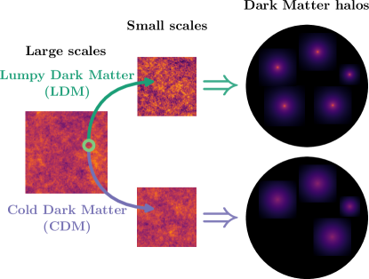
Figure 1: Depiction of Lumpy Dark Matter models, generated with cmbpy. Due to the enhanced power at small scales, in such models halos are more dense and abundant than in CDM.

We focus on DM models with enhanced structure at small scales. This is a natural prediction if DM is produced out of quantum fluctuations during inflation [22, 23, 24]. Even if these models do not require non-gravitational interactions between DM and baryons, limiting the detectability of DM in the laboratory, DM being produced out of small-scale isocurvature fluctuations entails significant substructure that may be tested. Similar effects are also predicted by primordial magnetic fields [25] or in non-standard inflationary models [26, 27, 28]. Because of the enhanced substructure, we name these DM models Lumpy Dark Matter (LDM).

Figure 1 previews the big picture. LDM models resemble CDM on large scales, but on small scales density fluctuations are greater. Consequently, when these fluctuations collapse to form DM halos, the larger fluctuation amplitudes in LDM result in more halos than in CDM. LDM halos also form earlier, when the Universe is denser, so their internal densities are higher. Our analysis probes both the increased abundance and densities, allowing us to determine the DM power spectrum with good precision at small scales, where to our knowledge only strong lensing determinations exist [29]. As usual in the literature, in this first study we use semianalytic techniques [30, 26, 31, 29]. Future work could improve on these results using simulation-based inference, ideally including baryons.

Quantitatively, LDM models are characterized by an enhanced primordial curvature power spectrum at small scales, that we parametrize as

$$\mathcal{P}_{\mathcal{R}}(k)\propto k^{n_{s}-1}\left[1+\left(k/k_{\mathrm{cut}}\right)^{n_{\mathrm{cut}}-n_{s}}\right]\,,$$ (1)

with $k$ comoving wavenumber, $n_{s}\simeq 0.97$ the standard CDM spectral index [1], $k_{\mathrm{cut}}$ the comoving wavenumber above which power is enhanced, and $n_{\mathrm{cut}}>n_{s}$ the enhanced spectral index. This expression interpolates from $\mathcal{P}_{\mathcal{R}}\propto k^{n_{s}-1}$ at $k\ll k_{\mathrm{cut}}$ to $\mathcal{P}_{\mathcal{R}}\propto k^{n_{\mathrm{cut}}-1}$ at $k\gg k_{\mathrm{cut}}$. Perturbations evolve as in CDM.

LDM models are phenomenologically interesting because, in contrast to most of the modified DM models studied in the literature [8, 9, 10, 11], the DM power spectrum is enhanced instead of suppressed. This opens new observational effects and channels with which to test them. In addition, some datasets suggest a “too many satellites” problem [32, 16, 33] that might point to such models.

The rest of the paper is organized as follows. In Section II, we quantify the impact of LDM models on DM halo properties. In Section III, we link to the properties of dwarf galaxies, discuss baryonic effects, and show that the correlation between galaxy kinematics and size is a sharp probe of DM substructure. In Section IV we describe our statistical analysis and results, and in Section V we conclude and point out future research directions. In the Appendices, we provide further details.

Below, we assume a Planck 2018 cosmology [1] (${h=67}$, $\Omega_{\mathrm{m}}=0.31$, $\sigma_{8}=0.81$, $\Omega_{\Lambda}=0.69$, $\Omega_{\mathrm{b}}=0.05$). We carry out DM calculations with the Galacticus [34] semi-analytic halo formation code. Unless otherwise specified, we evaluate Milky Way satellite properties at median infall redshift $z_{\mathrm{infall}}=1$ [35, 36, 37], i.e., when entering the Milky Way virial radius. We define halo virial masses as $M_{200c}$, i.e., the mean overdensity within the virial radius relative to the critical density is $\Delta=200$. We assume a Milky Way virial mass of $10^{12}\,M_{\odot}$ and concentration of $9$ [38]. We comment on these choices in Section III.

II Impact on dwarf galaxy halos

In this section, we use semi-analytic techniques to compute the impact of LDM models on DM halos. We show that enhanced power at small scales increases the number of low-mass halos and their central densities, leading to unique observational signatures in dwarf galaxies.

II.1 Formalism

We follow the extended Press-Schechter formalism [39, 40], which assigns DM halos to regions where density perturbations exceed a threshold. This formalism is expected to hold for a wide range of power spectra and cosmological models, and connects DM halos to the power spectrum through the variance of the density field

$$\sigma^{2}(R(M),z)\equiv\int\frac{\mathrm{d}^{3}k}{(2\pi)^{3}}P_{\mathrm{lin}}(k,z)|W(k,R)|^{2}\,,$$ (2)

where $R(M)\equiv\left[3M/(4\pi\bar{\rho}_{m})\right]^{1/3}$ is the Lagrangian radius of the halo with $M$ its mass and $\bar{\rho}_{m}$ the average matter density of the Universe, $z$ is redshift, $P_{\mathrm{lin}}$ is the linear matter power spectrum, and $W(k,R)$ is a window function that connects comoving wavenumber to Lagrangian radius. To avoid spurious halos at scales larger than those with enhanced power, we use a sharp $k$-space window [41]

$$W(k,R)=\theta\left(2.5/R-k\right)\,,$$ (3)

with $\theta$ the step function. Different window functions do not significantly change the results [42].

The number density of halos per unit mass, i.e., the halo mass function; is then

$$\frac{\mathrm{d}n_{\mathrm{halo}}}{\mathrm{d}M}=f(\sigma,z)\frac{\bar{\rho}_{m}}{M}\left|\frac{\mathrm{d}\log\sigma(R(M),z)}{\mathrm{d}M}\right|\,,$$ (4)

we use the Sheth-Tormen mass function $f$, that extends the Press-Schechter formalism to ellipsoidal collapse [43]

$$f(\sigma,z)=A\left[1+(a\nu)^{-p}\right]\sqrt{a}\,e^{-a\nu/2}/\sqrt{2\pi\nu}\,,$$ (5)

where $\nu\equiv\delta_{c}/\sigma(R,z)$ with $\delta_{c}$ the linear overdensity threshold for spherical collapse; and $A$, $a$, and $p$ are parameters calibrated to simulations. This formalism reproduces several non-CDM simulations [44], as well as CDM simulations down to halo masses $M\sim 10^{7}M_{\odot}$ [45]. Lower-mass halos are not expected to host galaxies and hence are not relevant for our analysis (see Section III.1). We set $\delta_{c}=1.686$, corresponding to an Einstein-de Sitter Universe; and $A=0.30$, $a=0.79$, and $p=0.22$ [46]. We add an overall 20% suppression due to baryons [47, 48, 49, 50]. As we are interested in Milky Way satellites, we need the subhalo mass function, which we compute following the merger tree algorithm from Refs. [51, 52, 53]. This algorithm describes the hierarchical formation history of DM halos. As we show below, our results do not strongly rely on the halo mass function, so potential uncertainties related to the extended Press-Schechter formalism in LDM models are subdominant contributions to our error budget.

We also explore halo density profiles. For low-mass halos, we assume an NFW form [54]

$$\rho(r)=\frac{\rho_{s}}{r/r_{s}\left(1+r/r_{s}\right)^{2}}\,,$$ (6)

with $\rho_{s}$ a characteristic density and $r_{s}$ the scale radius. For higher-mass halos, we include baryonic feedback by making the profiles cored as we describe in Section III.1. We parametrize $r_{s}$ in terms of the concentration

$$c_{200c}\equiv r_{\mathrm{vir}}/r_{s}\,,$$ (7)

with $r_{\mathrm{vir}}$ the virial radius. For fixed mass, halos with larger concentrations have larger central densities.

As already discussed in the original NFW paper, halo mass and concentration are not arbitrary. Instead, halos formed at higher redshift have higher concentrations at the present, reflecting that the average matter density of the Universe was larger at formation [54, 55, 56, 57]. This correlation was studied in detail by Diemer and Joyce [57], who proposed a semi-analytic relation between concentration, mass, power-spectrum slope, and formation redshift. This was shown to accurately reproduce the results of N-body simulations for a variety of masses, redshifts, and power spectra (see also Ref. [58]). Hence, we adopt the mass-concentration relation from Ref. [57]. When computing concentrations, we include a 16% lognormal scatter [59]; i.e., we assume that halo concentration follows a lognormal distribution with a median given by the relation in Ref. [57] and a standard deviation of 0.16 dex.

II.2 Consequences

The impact of enhanced power spectra on halo properties is now more explicit. From Eq. 2, enhanced power increases the variance of the density field $\sigma$, which leads to enhanced halo abundances, see Eqs. 4 and 5. Halos also form earlier, as can be understood from the collapsed mass fraction in extended Press-Schechter theory [60, 56],

$$M_{\mathrm{coll}}(z)=M_{0}\operatorname{erfc}\left(\frac{\delta_{c}\left/\left[\sqrt{2}(1-D(z_{0})/D(z))\right]\right.}{\sqrt{\sigma^{2}(fM_{0},z)-\sigma^{2}(M_{0},z)}}\right)\,,$$ (8)

with $M_{\mathrm{coll}}$ the mass of halo progenitors more massive than $fM_{0}$ that have collapsed by redshift $z$, $M_{0}\equiv M(z_{0})$ the final halo mass, and $D(z)$ the linear growth factor. As $M_{\mathrm{coll}}(z)$ is a growing function of $\sigma$, enhanced power leads to early halo formation, i.e., to high concentrations [26].

Below, we quantify both effects and show that the impact on halo concentrations is more dramatic. This can greatly affect the kinematics of galaxies inhabiting them.

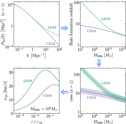
Figure 2: Impact of LDM models on halo structure. An enhanced power spectrum (top left) leads to early halo formation (top right), when the DM density is higher, leading to more concentrated halos (bottom right, shaded regions represent $1\sigma$ scatter) and higher internal velocities (bottom left).

Figure 2 shows that LDM models can significantly affect the internal halo kinematics due to the enhanced concentrations. For LDM, we set $k_{\mathrm{cut}}=8\,\mathrm{Mpc}^{-1}$ and $n_{\mathrm{cut}}=2.6$ (our analysis below excludes this). The top-right panel shows the redshift of halo formation computed following Ref. [56], defined as the redshift at which the mass within $r_{s}$ was contained in halo progenitors more massive than 2% of the final halo mass. The bottom-right panel shows halo concentrations computed following Ref. [57] as described above, along with 16% scatter [59]. The bottom-left panel shows the circular velocity curve, $v_{\mathrm{circ}}(r)=\sqrt{GM(<r)/r}$ with $G$ Newton’s constant, $M(<r)$ the enclosed mass, and $r$ radius; for fixed halo mass and an NFW profile. Other halos are similarly affected, but in a mass- and model-dependent way. These plots do not include tidal stripping or baryonic effects, that we introduce in Section III.1.

The results in Fig. 2 quantify the effects described above. If power is enhanced below a given scale, halos below a given mass will form earlier. This leads to large concentrations, i.e., large DM densities close to the halo center, implying large circular velocities.

A fortuitous cancellation increases the impact of modified power on the mass-concentration relation. For the currently favored nearly-scale-invariant power spectrum, at small scales $P_{\mathrm{lin}}(k)\propto k^{-3}$ approximately [61]. The integrand in Eq. 2 is then proportional to $k^{-1}$, and $\sigma(R)$ only grows logarithmically with $1/R$: at small scales $\sigma(R)$ “flattens out”, all halos form at similar redshifts, and thus have similar concentrations. Deviations from scale invariance such as those we consider induce a stronger dependence of $\sigma$ on $R$, greatly increasing the differences in formation time and concentration between halos.

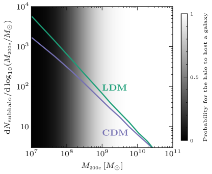
Figure 3: Impact of LDM models on the subhalo mass function. The grayscale shows the probability for halos to host galaxies in an illustrative model (we later set this free, see the text). The models we explore marginally affect visible subhalo abundance; our main observable is the enhanced concentrations.

Figure 3 shows that visible subhalo abundance is not much enhanced in the LDM models we explore. We show the $z=0$ subhalo mass function for a parent halo with Milky-Way mass, computed with Galacticus following Refs. [51, 52, 53] as described above. We use the same LDM parameters as in Fig. 2, $k_{\mathrm{cut}}=8\,\mathrm{Mpc}^{-1}$ and $n_{\mathrm{cut}}=2.6$. The background shows the halo occupation fraction, i.e., the probability for a DM halo to host a galaxy, from Ref. [36] (when performing our data analysis below, we set this free). $M_{200c}$ is the subhalo mass at infall; we discuss tidal effects and subhalo disruption in Section III.1.

The largest impact of LDM on halo abundances is on halos that are not expected to host galaxies: the subhalo mass function differs from CDM by $\sim 35\%$ at $10^{9}\,M_{\odot}$ and by $\sim 50\%$ at $10^{8}\,M_{\odot}$. Thus, our main observable is not total halo abundance, which we include for completeness and to lift degeneracies, but internal halo properties.

Overall, we conclude that LDM models strongly affect central densities of low-mass halos. Any kinematic probe of the inner part of such halos is thus a sensitive probe of LDM models. In the following, we follow the procedure in Ref. [21], extending the code dis to predict and observationally probe Milky Way satellite circular velocities and sizes, linking them to the DM power spectrum.

III Impact on Milky Way satellites

In this section, we link low-mass DM halo properties to dwarf galaxy properties. We show that enhanced power predicts a characteristic relation between stellar kinematics and galaxy size, that can be observationally explored.

As mentioned in Section I, we fix the Milky Way mass to $10^{12}\,M_{\odot}$ and evaluate satellite properties at median infall redshift. As we show in Appendices B and A, the impact of leaving these free in our analysis is negligible, as other free parameters dominate our error budget. We also neglect specific aspects of the Milky Way merger history, like the Large Magellanic Cloud. Although recent work shows that it can impact satellite counts [62, 63, 64, 65], the effect is smaller than our overall error budget (see Appendix B). On top of that, we use satellites discovered by SDSS, whose footprint does not contain the Magellanic Clouds. If other constraints are improved in future work, or if satellites recently discovered in the Southern Hemisphere are included [66, 67, 68, 69, 70, 71, 72, 73, 74, 75, 76, 77, 78], this may need revisiting.

III.1 Formalism

It is challenging to directly observe low-mass DM halos. Avenues include gravitational lensing [32], already quite mature (see e.g., Refs. [79, 80, 81, 82, 83, 84]); perturbations to the Milky Way stellar disk [85, 86]; or disruption of stellar streams [87, 88, 89]. These may probe halos smaller than those that host galaxies. Yet observing the dwarf galaxies that low-mass halos host provides unique access to their central regions. This, as shown above in Fig. 2, is a sharp probe of LDM models. Dwarf galaxies are also DM-dominated [90, 91], alleviating baryonic uncertainties that are more significant for more massive galaxies.

Below, we describe how we use the output from Galacticus (subhalo masses, concentrations, and total abundance) to build a Milky Way satellite galaxy population. To probe the central kinematics affected by LDM models, we need to predict the relationship among galaxy sizes, internal velocities, and observational abundance.

We quantify the size of a galaxy by its 2D-projected half-light radius [21], that we denote as $R_{\mathrm{eff}}$. It is correlated with its stellar mass $M_{*}$ by a scaling relation,

$$\log_{10}\left(R_{\mathrm{eff}}/\mathrm{kpc}\right)=0.268\log_{10}\left(M_{*}/M_{\odot}\right)-2.11\,.$$ (9)

This relation has 23.4% lognormal scatter. It was obtained in Ref. [21] using isolated dwarf data [92, 93], and it is similar to the relation found for satellites in the Local Group [94] and in simulations [95]. Although this relation can have uncertainties at low $R_{\mathrm{eff}}$ due to selection effects related to surface brightness, this does not significantly affect our error budget as we discuss next.

The stellar mass $M_{*}$, in turn, links to the infall halo mass [96] $M_{200c}$ via the stellar mass-halo mass relation, that we parametrize as a power law

$$M_{*}=M_{200c}\,\mathcal{N}\left(\frac{M_{200c}}{M_{0}}\right)^{\beta^{M_{*}}}\,,$$ (10)

with $\mathcal{N}$ a constant, $M_{0}$ a reference mass, and $\beta^{M_{*}}$ the power-law slope. At dwarf galaxy masses this relation is poorly constrained, and most relations are calibrated at higher mass and then extrapolated [96, 36, 97, 98] (see, however, Refs. [99, 100, 64]). At $z=1$, Ref. [96] found $\mathcal{N}=0.046$, $M_{0}=1.5\times 10^{12}M_{\odot}$, and $\beta^{M_{*}}=0.96$. The scatter in this relation is also uncertain and potentially mass-dependent [101, 102, 103, 98]; we parametrize it as

$$\sigma(M_{*})=\sigma^{M_{*}}+\gamma^{M_{*}}\log_{10}\frac{M_{200c}}{10^{11}\,M_{\odot}}\,.$$ (11)

In our data analysis below, we set $\beta^{M_{*}}$, $\sigma^{M_{*}}$, and $\gamma^{M_{*}}$ to be free parameters. Thus, uncertainties on the $R_{\mathrm{eff}}$-$M_{*}$ relation do not significantly affect our error budget (see also Appendix B). This also allows us to observationally explore the low-mass stellar mass-halo mass relation.

We quantify internal velocity by the line-of-sight stellar velocity dispersion $\sigma_{\mathrm{los}}^{*}$. We use the estimator from Ref. [104]

$$\sigma_{\mathrm{los}}^{*}=\sqrt{\frac{G}{4}\frac{M(<r_{1/2})}{R_{\mathrm{eff}}}}\,,$$ (12)

with $M(<r_{1/2})$ the mass enclosed by the 3D half-light radius $r_{1/2}=R_{\mathrm{eff}}/0.75$ (this is accurate for a wide variety of stellar distributions [104]). Other estimators produce very similar results [21], see Appendix A. $M(<r)$ only includes DM, as the stellar mass is subdominant [90, 91].

$\sigma_{\mathrm{los}}^{*}$ links to halo concentration through the density profile entering $M(<r)$, which in large-mass halos can be affected by baryonic feedback that turns central NFW “cusps” predicted by DM simulations into “cores” [105, 106, 107, 108, 109, 110, 111, 112, 113, 114]. We include this by setting cored profiles above a threshold halo mass $M^{\mathrm{core}}_{\mathrm{thres}}$. We use the simulation- and observation-constrained profile from Ref. [115], where the core size depends on the time over which a galaxy has formed stars, assuming that satellites stop forming stars at infall. $M^{\mathrm{core}}_{\mathrm{thres}}$ is uncertain [21], so in our data analysis below we set it to be a free parameter. This allows us to observationally explore the cusp-core transition.

The Milky Way gravitational field can tidally strip DM halos, changing their density profile. To implement this, the density profile can be truncated beyond the tidal radius [116, 83, 29], defined as the radius where the Milky Way tidal force balances the attractive force of the satellite galaxy [117]. Even inside the tidal radius, structural halo parameters get modified through tidal shocking and heating [118, 119, 120, 121, 122, 123, 124, 125]. As we show in Appendix A, the impact of tidal stripping on our analysis is negligible, as other free parameters dominate our error budget. This is because our observables are sensitive to halo properties inside the half-light radius, usually smaller than the tidal radius; and because galaxies remain unaffected until their DM halos lose more than 90% of their mass [21, 126, 127] (our population study is sensitive to average properties, and the average mass loss of Milky Way satellites is estimated to be $\sim 30\%$ [128, 129, 130]). The high concentrations of LDM halos may also make them more resilient to tidal stripping [120, 131]; further work is needed to assess this.

Regarding observational abundance, not all DM halos are expected to host galaxies. Only those more massive than $10^{7}$–$10^{8}\,M_{\odot}$ by reionization would have gas that can cool and form stars [132, 133, 134]. We include this via the halo occupation fraction, i.e., the probability for a halo to host a galaxy, that we parametrize as a sigmoid function

$$\operatorname{hof}(M_{200c})=\frac{1/2+\operatorname{erf}\left(\alpha^{\mathrm{hof}}\log_{10}\left[M_{200c}/M_{0}^{\mathrm{hof}}\right]\right)}{2}\,,$$ (13)

with $\operatorname{erf}$ the error function, $M_{0}^{\mathrm{hof}}$ the mass below which halos do not host galaxies, and $\alpha^{\mathrm{hof}}$ a parameter controlling the steepness of the transition. With simulation and semi-analytic modelling, Refs. [135, 36] found $\alpha^{\mathrm{hof}}=1.3$ and $M_{0}^{\mathrm{hof}}=10^{8.4}\,M_{\odot}$; there are also observational limits from the Milky Way satellite luminosity function [64, 17]. In our data analysis below, we set $\alpha^{\mathrm{hof}}$ and $M_{0}^{\mathrm{hof}}$ to be free parameters. This allows us to observationally determine the low-mass halo occupation fraction.

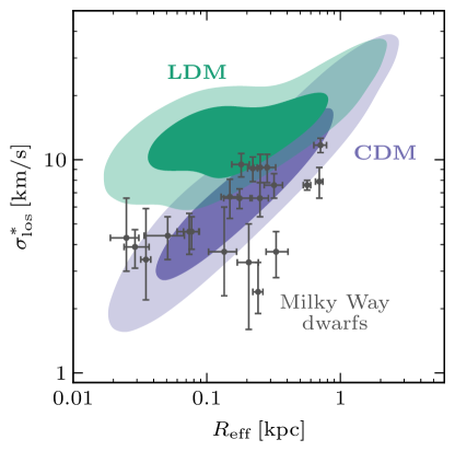
Figure 4: Correlation between stellar velocity dispersion and half-light radius, and data from classical and SDSS Milky Way dwarfs. Colored regions enclose 68% and 95% of the predicted population, for an illustrative model connecting halos to galaxies (see Section III.2, we later set this free). Data disfavors the high velocity dispersions of LDM models.

Not all halos hosting galaxies are observable either: for a given survey, faint and distant galaxies will escape detection. We account for this by assigning to each galaxy with stellar mass below $4\times 10^{5}\,M_{\odot}$ (brighter galaxies correspond to classical satellites) an observation probability

$$\mathcal{P}_{\mathrm{obs}}=\frac{\int_{V_{\mathrm{obs}}(L)}n(\vec{r})\,\mathrm{d}^{3}r}{\int_{V_{\mathrm{vir}}}n(\vec{r})\,\mathrm{d}^{3}r}\equiv\frac{1}{\mathcal{C}(L)}\,,$$ (14)

with $n$ the number density of satellites, $V_{\mathrm{vir}}$ the virial volume of the Milky Way, and $V_{\mathrm{obs}}(L)$ the volume where satellites of luminosity $L$ can be detected by the survey. $\mathcal{C}(L)$ is the luminosity-dependent completeness correction [16]. We assume that $n(\vec{r})$ does not change significantly with the solid angle, so that the selection function is separable into a radial and an angular component

$$\mathcal{C}(L)\equiv\mathcal{C}_{\Omega}\,\mathcal{C}_{r}\,;\hskip 3.0pt\mathcal{C}_{\Omega}\equiv\frac{4\pi}{\Omega}\,;\hskip 3.0pt\mathcal{C}_{r}\equiv\frac{\int_{0}^{r_{\mathrm{vir}}}n(r)r^{2}\,\mathrm{d}r}{\int_{0}^{r_{\mathrm{c}}(L)}n(r)r^{2}\,\mathrm{d}r}\,,$$ (15)

with $\Omega$ the angular coverage of the survey, $r_{\mathrm{vir}}$ the Milky Way virial radius, and $r_{\mathrm{c}}(L)$ the largest distance at which satellites of luminosity $L$ can be observed by the survey. We consider classical and SDSS satellites; for the latter $\Omega_{\mathrm{SDSS}}=3.65\,\mathrm{sr}$ and $r_{\mathrm{c}}$ is given by [136, 137]

$$r_{\mathrm{c}}(L)=1.5\,\mathrm{kpc}\,\left(L/L_{\odot}\right)^{0.51}\,.$$ (16)

We compute luminosities assuming $M_{*}/M_{\odot}=2L/L_{\odot}$, appropriate for old stellar populations [104, 138]. $\mathcal{C}_{\Omega}$ has 19% scatter due to anisotropy [13].

Tidal subhalo disruption affects the radial distribution of satellites $n(r)$, which is hence very uncertain [16, 139, 140, 141, 142, 143, 144, 50, 49, 145, 103]. This made it a big systematic uncertainty in previous work of satellite populations [16, 64]. To be conservative, we are agnostic about tidal disruption and parametrize $n(r)$ as

$$n(r)=n_{\mathrm{GK17}}(r)+y_{\mathcal{C}}[n_{\mathrm{NFW}}(r)-n_{\mathrm{GK17}}(r)]\,,$$ (17)

with $y_{\mathcal{C}}\in[0,1]$ a parameter that interpolates between an unstripped NFW distribution, $n_{\mathrm{NFW}}(r)$ — i.e., satellites follow the DM halo distribution —, and the strongly tidally disrupted distribution from Ref. [139], $n_{\mathrm{GK17}}(r)$. In our data analysis below, we set $y_{\mathcal{C}}$ free, which allows us to observationally explore tidal subhalo disruption.

III.2 Consequences

Figure 4 illustrates how the large concentrations predicted in LDM models become imprinted on galaxies in the form of high stellar velocity dispersions, which can be in tension with Milky Way satellite data. We plot the correlation between $\sigma_{\mathrm{los}}^{*}$ and $R_{\mathrm{eff}}$ of Milky Way satellites. We generate the theoretical expectations by sampling halo masses from the product of the subhalo mass function described in Section II.1 and the halo occupation fraction from Ref. [36], and sampling halo concentrations as described in Section II.1. We use the same LDM parameters as in Figs. 2 and 3, $k_{\mathrm{cut}}=8\,\mathrm{Mpc^{-1}}$ and $n_{\mathrm{cut}}=2.6$ (our analysis below excludes this). We assign $R_{\mathrm{eff}}$ and $\sigma_{\mathrm{los}}^{*}$ using Eqs. 12 and 9. $R_{\mathrm{eff}}$ depends on the stellar mass, that we generate using the stellar mass-halo mass relation from Ref. [96] with lognormal scatter of 0.15 dex [96]. $\sigma_{\mathrm{los}}^{*}$ depends on the halo density profile: following Ref. [21], we assume cored profiles for halo masses above $M_{\mathrm{thres}}^{\mathrm{core}}=10^{9}M_{\odot}$. Finally, we weight each galaxy by its observation probability $\mathcal{P}_{\mathrm{obs}}$, computed with Eq. 14 assuming an undisrupted NFW spatial distribution of satellites. Data correspond to classical and SDSS satellites, as obtained from Ref. [92]. In our data analysis below, we allow the parameters of the stellar mass-halo mass relation, the halo occupation fraction, the halo mass where baryonic feedback switches the profiles from NFW to cored, and the amount of tidal subhalo disruption to vary; this significantly affects the predicted population (see Appendix A). It also increases the agreement of data with CDM, although our choices for Fig. 4 are within the 2$\sigma$ allowed region (see Appendix C).

As we see from Fig. 4, velocity dispersion $\sigma_{\mathrm{los}}^{*}$ is correlated with half-light radius $R_{\mathrm{eff}}$. Galaxies with low $R_{\mathrm{eff}}$ are less massive (see Eqs. 10 and 9), which leads to lower $\sigma_{\mathrm{los}}^{*}$ (see Eq. 12). However, $\sigma_{\mathrm{los}}^{*}$ also depends on the central density, i.e., on the halo concentration. As in LDM models low-mass halos have higher concentrations than in CDM, LDM predicts higher $\sigma_{\mathrm{los}}^{*}$ at low $R_{\mathrm{eff}}$.

These results highlight that taking into account stellar kinematics and their correlation with the half-light radius is a powerful observational probe of the DM power spectrum. Below, we carry out a statistical analysis of classical and SDSS Milky Way satellites to quantify this.

IV Statistical analysis and results

The procedure described above allows us to predict the number of visible Milky Way satellites, as well as their line-of-sight stellar velocity dispersions $\sigma_{\mathrm{los}}^{*}$ and half-light radii $R_{\mathrm{eff}}$, for CDM and LDM models. In this section, we use observational data to infer the primordial DM power spectrum and the galaxy-halo connection parameters.

We fit for the total number of classical and SDSS Milky Way satellites, their velocity dispersions, and half-light radii, as obtained from Ref. [92]; using an unbinned likelihood described in detail in Appendix B. We generate theoretical predictions with Galacticus, for DM halo properties; and dis, for galaxy properties; as described in Sections II and III. Our free parameters are $\{k_{\mathrm{cut}},\,n_{\mathrm{cut}}\}$, that describe the DM power spectrum; {$\beta^{M_{*}}$, $\sigma^{M_{*}}$, $\gamma^{M_{*}}$, $\alpha^{\mathrm{hof}}$, $M_{0}^{\mathrm{hof}}$, $M_{\mathrm{thres}}^{\mathrm{core}}$}, that describe the galaxy-halo connection; and $y_{\mathcal{C}}$, that parametrizes tidal disruption of Milky Way subhalos. In addition, the anisotropy of the satellite distribution has 19% scatter [13]. We include this by multiplying $\mathcal{C}_{\Omega}$ in Eq. 15 with a free parameter $\sigma_{\mathcal{C}_{\Omega}}$ and adding a Gaussian prior on $\sigma_{\mathcal{C}_{\Omega}}$ centered at 1 and with a width of 0.19. $\sigma_{\mathcal{C}_{\Omega}}$ is the last free parameter of our analysis.

We perform a frequentist analysis to avoid prior dependence and Bayesian volume effects. We expect these effects because some parameters are not strongly constrained by our analysis, there are non-trivial correlations, and part of the parameter space is unbounded.

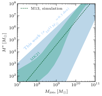
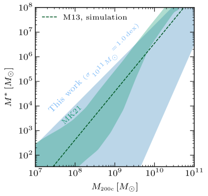
Figure 5: Stellar mass-halo mass relation allowed by our analysis within $2\sigma$, for different fixed scatters at high mass, together with the simulation prediction that we use in Fig. 4 (Moster et al. 2013, M13 [96]) and previous constraints (Manwadkar and Kravtsov 2021, MK21 [100]). Increased scatter suppresses the median stellar mass to avoid overproducing bright galaxies. The lower mass end is degenerate with the halo occupation fraction and is hence more uncertain.

IV.1 Galaxy properties

Our analysis constrains the relation between galaxies and DM halos with minimal assumptions on baryonic physics and the small-scale DM power spectrum. Below, we describe our inferences on the stellar mass-halo mass relation, the halo occupation fraction, and the amount of subhalo tidal disruption by the Milky Way. We provide the full results of the analysis in Appendix C.

Figure 5 shows the stellar mass-halo mass relation allowed by our analysis within $2\sigma$, compared against observational constraints using the luminosity function [100] (which includes DES and PS1 satellites on top of SDSS and classical satellites, assumes a standard CDM power spectrum, and uses a model for galaxy luminosity and halo occupation fraction), and the extrapolated predictions from the simulation of Ref. [96]. Since we describe the stellar mass-halo mass relation in terms of three parameters — the median power-law slope, the scatter at $10^{11}\,M_{\odot}$, and the growth of scatter at low mass, see Eqs. 10 and 11 — and we find significant correlations (see Appendix C), we show the allowed relation for two fixed values of the scatter at $10^{11}\,M_{\odot}$: 0.1 dex and 1 dex. Other parameters, including those controlling the DM power spectrum, are allowed to vary freely.

Our median results are compatible with extrapolation from simulation [96]. We see that the median power-law slope is strongly correlated with scatter: if scatter is high, the median stellar mass of low-mass halos has to be small. Otherwise, too many visible satellite galaxies would be predicted. This allows us to obtain a quite robust upper limit on the largest stellar mass of low-mass halos, consistent with previous work [100].

The smallest stellar mass of low-mass halos, however, is worse-constrained by our analysis. This is because decreasing the stellar mass would predict less visible satellites, which is partly degenerate with increased halo occupation fraction. A priori information on the halo occupation fraction (as in Ref. [100]) would break this degeneracy; we comment on this in the Conclusions.

We also conclude that the uncertain stellar mass-halo mass relation should not strongly affect our determination of the DM power spectrum. The main observable for the stellar mass-halo mass relation is the number of observed satellites, whereas the power spectrum is determined mainly from the correlation between stellar velocity dispersion and half-light radius, see Fig. 4. There is only a mild degeneracy because by making low-mass halos brighter, the average velocity dispersion in LDM models can be somewhat reduced. The correlations in our full analysis in Appendix C confirm this intuition.

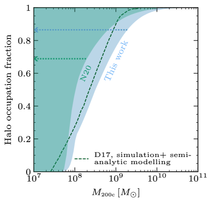
Figure 6: Halo occupation fraction allowed by our analysis within $2\sigma$, the prediction used in Fig. 4 (Dooley et al. 2017, D17 [36]), and previous constraints (Nadler et al. 2020, N20 [64]). Regions within the arrows are allowed. Our analysis informs on halo occupation at masses above $\sim 10^{8}\,M_{\odot}$.

Figure 6 shows the halo occupation fraction allowed by our analysis within $2\sigma$, together with existing constraints using the luminosity function [64] (using DES and PS1 dwarfs and assuming a standard CDM power spectrum), and the relation inferred in Refs. [135, 36] by combining simulation with semi-analytic modelling (see also Refs. [17, 98]). All the region within the arrows is allowed. Other parameters, including those controlling the DM power spectrum, are allowed to vary freely.

We observe that data requires halos with masses between $10^{8}M_{\odot}$ and $10^{10}M_{\odot}$ to host galaxies. This is consistent with the results from recent simulations and the luminosity function: if these halos did not host galaxies, there would be a “too many satellites” problem. Our analysis is unable to robustly decide if lower-mass halos have a non-zero probability of not hosting galaxies (i.e., if their halo occupation fraction is different from 0), as this effect is degenerate with a modified stellar mass-halo mass relation: very low-mass halos can host galaxies if these galaxies are very dim.

In our analysis, the halo occupation fraction is mildly degenerate with the DM power spectrum, as by populating low-mass halos the average velocity dispersion in LDM models can be reduced. However, the additional handle from the total number of galaxies together with the different correlation between $\sigma_{\mathrm{los}}^{*}$ and $R_{\mathrm{eff}}$ in LDM and CDM models (see Fig. 4) alleviate this effect.

Regarding tidal subhalo disruption and the radial satellite distribution in Eqs. 14, 15 and 17, we find $y_{\mathcal{C}}\gtrsim 0.3$ at $1\sigma$ (see Appendix C). I.e., our analysis disfavors strong tidal disruption found in simulation [139], as that would produce a “too many satellites” problem [16].

IV.2 Dark Matter properties

We now turn to the original purpose of this paper: what do Milky Way satellite properties tell us about the DM power spectrum at the smallest scales?

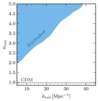
Figure 7: Excluded values of LDM parameter space in our analysis within 2$\sigma$. Dwarf galaxy velocity dispersions and sizes probe dark matter substructure for 5 Mpc${}^{-1}\lesssim k\lesssim$ 40 Mpc^-1.

Figure 7 shows that the DM power spectrum cannot be strongly enhanced between comoving scales 5 Mpc${}^{-1}\lesssim k\lesssim$ 40 Mpc^-1 (as large values of the power-spectrum slope $n_{\mathrm{cut}}$ are excluded). We show the $2\sigma$ excluded values of $k_{\mathrm{cut}}$ and $n_{\mathrm{cut}}$, allowing other parameters to vary freely.

The results are intuitive: from Fig. 4, data approximately follow the CDM correlation between $\sigma_{\mathrm{los}}^{*}$ and $R_{\mathrm{eff}}$, with no clear sign of a break characteristic of LDM. This favors similar concentrations for all Milky Way satellites, i.e., similar formation times. As explained in Section II.2, this favors close-to-scale-invariant power spectra.

Our analysis loses sensitivity for $k_{\mathrm{cut}}\lesssim 5\,\mathrm{Mpc^{-1}}$ and ${k_{\mathrm{cut}}\gtrsim 40\,\mathrm{Mpc^{-1}}}$. This is intuitive: using Eq. 3, smaller $k$ correspond to halo masses $M_{200c}\gtrsim 10^{11}M_{\odot}$, above the mass of a Milky Way satellite galaxy. Larger $k$ correspond to halo masses $M_{200c}\lesssim 10^{8}M_{\odot}$. The dwarfs with lowest half-light radii that we consider (Segue-I, Segue-II and Willman-I) have ${M_{*}\simeq 2\text{--}5\times 10^{2}M_{\odot}}$, i.e., halo masses in that ballpark (see Fig. 5).

Our determination of the power spectrum is robust against baryonic effects and different galaxy-halo connection models. The strongest degeneracy we find is with the halo mass above which baryonic feedback makes DM density profiles cored, $M_{\mathrm{thres}}^{\mathrm{core}}$. By making low-mass halos cored, their velocity dispersion gets reduced, and LDM predictions resemble more those of CDM. However, a CDM-like correlation between $\sigma_{\mathrm{los}}^{*}$ and $\mathrm{R}_{\mathrm{eff}}$ (see Fig. 4) is never fully mimicked. Data can tell apart LDM and CDM even if LDM halos are cored at all halo masses.

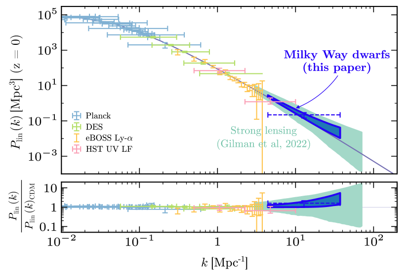
Figure 8: Allowed linear matter power spectrum in our analysis within 1$\sigma$ (shaded), and its geometric mean (dashed data point). Dwarf galaxy velocity dispersion and size data is a unique, sharp probe of small-scale dark matter properties.

Figure 8 shows that dwarf galaxy velocities and sizes determine the DM power spectrum at small scales with unprecedented precision. We show existing measurements from Planck [146], DES [147], eBOSS Lyman-$\alpha$ [3], the UV luminosity function as measured by the Hubble Space Telescope [31], and strong gravitational lensing [29]; the first three measurements have been obtained using the mpk_compilation code [148]. Since our parametrization in Eq. 1 only allows for enhanced power spectra, for consistency we have also made sure that the analysis does not prefer suppressed power spectra. We parametrize suppressed power with $n_{\mathrm{cut}}<n_{s}$ as $\mathcal{P}_{\mathcal{R}}(k)\propto k^{n_{s}-1}\left/\left[1+\left(k/k_{\mathrm{cut}}\right)^{n_{s}-n_{\mathrm{cut}}}\right]\right.$. This expression smoothly interpolates from $\mathcal{P}_{\mathcal{R}}\propto k^{n_{s}-1}$ at $k\ll k_{\mathrm{cut}}$ to $\mathcal{P}_{\mathcal{R}}\propto k^{n_{\mathrm{cut}}-1}$ at $k\gg k_{\mathrm{cut}}$.

The dark shaded area in Fig. 8 encloses all power spectra in our 1$\sigma$ allowed region for {$k_{\mathrm{cut}}$, $n_{\mathrm{cut}}$}, and the dashed data point is its geometric mean. Quantitatively,

$$\frac{P_{\mathrm{lin}}}{P_{\mathrm{lin}}^{\mathrm{CDM}}}=1.61\pm 0.55\,,$$ (18)

for $4\,\mathrm{Mpc^{-1}}<k<37\,\mathrm{Mpc^{-1}}$. The range in $k$ is where our analysis provides significant constraints. For other values of $k$, our uncertainties increase rapidly.

Our results are somewhat stronger than, and complementary to, the strong lensing determination in Ref. [29], which has different model assumptions and uncertainties. We find a slight $\sim 1\sigma$ preference for enhanced power, which is a consequence of the slight “turn up” of velocity dispersions at low $R_{\mathrm{eff}}$ in Fig. 4. This effect, however, is not statistically significant.

Overall, our results add a high-precision, small-scale handle to the global picture of the primordial DM power spectrum being almost-scale-invariant across 6 orders of magnitude in wavenumber. We do so by exploiting sizes and kinematics of one of the smallest DM-dominated class of systems we know of: Milky Way satellite galaxies.

V Conclusions and future directions

The properties of DM at small scales remain uncertain. In this paper, we have shown that the correlation between dwarf galaxy internal velocities and sizes is a powerful probe to explore them. Our constraining power mostly comes from probing the concentration-mass relation of DM halos, in contrast to previous work focusing on halo abundances [18, 20, 13, 14, 15, 16, 17, 18, 19, 20].

We focus on models that enhance the primordial matter power spectrum at small scales, that we denote as “Lumpy Dark Matter” (LDM). This prediction is natural if DM is produced out of quantum fluctuations during inflation, which does not require non-gravitational interactions with baryons [22, 23, 24]. We utilize semi-analytic techniques and scaling relations, inspired by physics models and calibrated against simulations, to compute DM halo properties. We are agnostic about many aspects of the galaxy-halo connection, allowing us to marginalize over poorly understood baryonic effects, and carry out a joint analysis of internal velocities, sizes, and total abundance of classical and SDSS Milky Way satellites.

Regardless of the DM power spectrum, we constrain the stellar mass-halo mass relation, the halo occupation fraction, and tidal subhalo disruption. We find that halos with masses of $10^{8}M_{\odot}$ and $10^{9}M_{\odot}$ must host galaxies with stellar masses below $10^{4}M_{\odot}$ and $10^{6}M_{\odot}$, respectively; and our analysis disfavors strong tidal disruption. This is mostly inferred from the total satellite abundance, implying little correlation with our determination of DM properties that relies mostly on the correlation between stellar velocity dispersion and half-light radius.

We obtain a leading-precision determination of the DM power spectrum on sub-galactic scales $4\,\mathrm{Mpc^{-1}}<k<37\,\mathrm{Mpc^{-1}}$. Milky Way satellite properties imply that, at those scales, the DM power spectrum cannot deviate from scale invariance by more than a factor $\sim 2$ at $1\sigma$.

Our methodology can be easily extended in further work. On the DM side, many scenarios that modify the small-scale DM properties have been explored in the literature. Examples include Self-Interacting Dark Matter (SIDM) [8], Warm Dark Matter (WDM) [9, 10], Fuzzy Dark Matter (FDM) [11], or a modified cosmological history [149, 150]. They are theoretically and observationally motivated, and in many of them the power spectrum at small scales is suppressed. Their consequences for the correlation between velocity dispersions and half-light radii are unexplored. The fact that our analysis finds a slight preference for enhanced power spectra forecasts increased sensitivity to such models.

On the modeling side, in this paper we have been agnostic about the galaxy-halo connection. However, there exist physically motivated models that predict the stellar mass-halo mass relation and the halo occupation fraction, as a function of halo concentration and assembly history [134, 151, 152]. Adding that information would improve the sensitivity to DM properties. For instance, higher concentration and earlier halo formation in LDM models may increase the stellar mass and the probability to host a galaxy (as halos would be more massive before reionization and may form stars more efficiently), contradicting observations. Our data analysis methodology presented here can also be used to test galaxy formation models. As mentioned in the Introduction, future work can also improve on the results presented here by running LDM simulations of halo and galaxy formation and evolution, that could be tailored to the Milky Way assembly history and include the associated uncertainties.

On the observational side, there is plenty of room for increased precision. We have only included classical and SDSS satellites (whose observations could be improved [129]), but our analysis can be extended to include Milky Way satellites discovered by the Dark Energy Survey, for which we are starting to get kinematic data (see, e.g., Refs [66, 67, 68, 69, 70]) and whose completeness correction is understood [153]; Milky Way satellites discovered by DELVE [71, 72, 73, 74, 75]; M31 satellites, to avoid the possibility of the Milky Way being an outlier; or even field dwarfs, unaffected by host galaxy effects but whose completeness correction and DM-driven velocity dispersion is harder to model. In the future, the Rubin Observatory should discover many dwarfs, within and outside the Milky Way, and inform on their spatial distribution [154, 155].

The satellite luminosity function can also be added to our dataset. This would better constrain the stellar mass-halo mass relation and the halo occupation fraction. Abundances, luminosities, sizes, and kinematics are the galaxy observables that most directly relate to DM halo features. Analyzing them together would provide a more complete picture of DM properties.

Finally, LDM models have a rich phenomenology that can be explored with other observables. As Fig. 2 shows, enhanced power spectra dramatically increase the formation redshift of low-mass halos, by breaking a fortuitous cancellation in the density variance of scale-invariant power spectra. This may produce stars early and affect reionization, which can be explored with Cosmic Microwave Background [156, 1, 157] and 21 cm observations [158]. Current observations from JWST are also providing a unique window to the high-redshift Universe and the formation of the first galaxies [159, 160, 161, 162, 163, 164, 165, 166, 167, 168, 169, 170, 171]. Determining the UV luminosity function can thus be a sharp probe of the DM power spectrum, as shown by existing work with HST data [31, 172].

Evidence for an unknown Dark Matter, five times more abundant than regular matter, first appeared in galaxy observations [173, 174]. This was confirmed to high accuracy observing the largest scales of our Universe [175, 1]. By studying back small-scale Dark Matter-dominated systems with increased precision, we are now on our way to building a coherent picture of the properties of the second most abundant component of the Universe.

Appendix A Impact of tidal stripping, subhalo infall times, the velocity estimator, and baryonic feedback

In this Appendix, we quantify the approximations described in the main text. We show that including tidal stripping, the different subhalo infall times, or a different $\sigma_{\mathrm{los}}^{*}$ estimator affects our observables less than the observational uncertainties and than the parameters that we set free —baryonic feedback that turns cusps into cores, the stellar mass-halo mass relation, the halo occupation fraction, and subhalo tidal disruption. If constraints on the latter are improved in future work and they stop dominating the error budget, these approximations may need revisiting.

A.1 Tidal stripping

In the main text, we neglect tidal stripping of subhalos by the Milky Way.

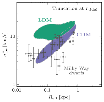
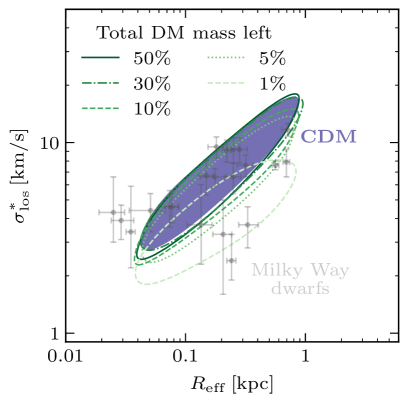
Figure A1: Same as Fig. 4, but the dashed lines include tidal effects. To avoid crowding the figure, colored regions show 68% of the enclosed population. In the left panel, we truncate DM density profiles at the tidal radius. In the right panel, we include tidal shocking and heating by changing the halo structural parameters, following the “tidal tracks” in Ref. [123]. Tidal effects would have a subleading impact on our error budget.

Figure A1 shows that tidal effects have a subleading impact on our observables. Both panels show the correlation between $\sigma_{\mathrm{los}}^{*}$ and $R_{\mathrm{eff}}$, together with data from classical and SDSS satellites, for the same halo-galaxy connection model and LDM parameters as Fig. 4, but including tidal effects in the dashed regions. In the left panel, we truncate the halo density profile beyond the tidal radius [116, 83, 29], as computed with Galacticus following Ref. [176]. In the right panel, we include tidal shocking and heating effects by changing halo structural parameters following the “tidal tracks” in Ref. [123]. We show only the CDM scenario to which Ref. [123] was calibrated. As mentioned in the main text, high concentrations of LDM halos may make them more resilient to tidal stripping [120, 131], so similar or smaller effects are expected for LDM.

We observe that DM mass removal beyond the tidal radius has a negligible impact on our observables given the precision of the data (see Fig. A4 below for the impact of the parameters that we set free). Tidal shocking and heating could have a significant impact, but this would require a large fraction of the DM halo population to lose more than $95\%$–$99\%$ of their mass. Simulations [128, 130] and observations [129] disfavor such dramatic effects. Similar conclusions were reached in previous population studies: dwarf galaxies are located well inside their host DM halos, so very strong tidal stripping at the population level is needed to affect the conclusions [21, 126, 127].

A.2 Infall times

In the main text, we evaluate all Milky Way satellite properties at median infall redshift $z_{\mathrm{infall}}=1$ [35, 36, 37].

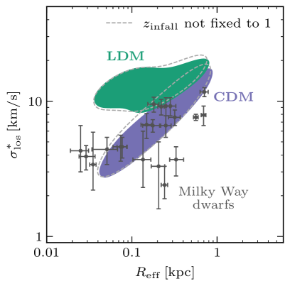
Figure A2: Same as Fig. 4, but the dashed lines include the different satellite infall times. To avoid crowding the figure, colored regions show 68% of the enclosed population. Different infall times would have a subleading impact on our error budget.

Figure A2 shows that including the different infall redshifts has a subleading impact on our observables. We show the correlation between $\sigma_{\mathrm{los}}^{*}$ and $R_{\mathrm{eff}}$, together with data from classical and SDSS satellites, for the same halo-galaxy connection model and LDM parameters as Fig. 4, but evaluating halo properties at infall redshift as computed with Galacticus in dashed.

We observe that the impact on our observables is negligible given the precision of the data (see Fig. A4 below for the impact of the parameters that we set free). The main effect is to slightly increase $\sigma_{\mathrm{los}}^{*}$. This is because the $z_{\mathrm{infall}}$ distribution is skewed towards $z_{\mathrm{infall}}>1$ [35, 36, 37], and internal halo velocities are higher at high redshift [21].

A.3 Velocity estimator

In the main text, we estimate $\sigma_{\mathrm{los}}^{*}$ using Eq. 12, that was obtained in Ref. [104]. This was shown to be robust against stellar velocity dispersion anisotropy. Ref. [177] proposed a different estimator, also robust against the shape of the inner halo profile and how deeply the stellar component is embedded within the halo. By comparing with simulation, the latter estimator was shown to have an accuracy of $\sim 10\%$ (better than our observational uncertainties).

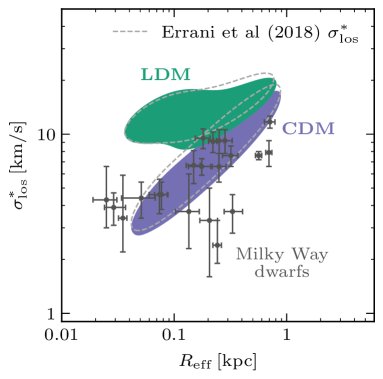
Figure A3: Same as Fig. 4, but the dashed lines use the $\sigma_{\mathrm{los}}^{*}$ estimator from Ref. [177]. To avoid crowding the figure, colored regions show 68% of the enclosed population. A recent mass estimator would have a subleading impact on our error budget.

Figure A3 shows that using the estimator from Ref. [177] has a subleading impact on our observables. We show the correlation between $\sigma_{\mathrm{los}}^{*}$ and $R_{\mathrm{eff}}$, together with data from classical and SDSS satellites, for the same halo-galaxy connection model and LDM parameters as Fig. 4, but with the estimator from Ref. [177] in the dashed regions.

We observe that the impact on our observables is negligible given the precision of the data (see Fig. A4 below for the impact of the parameters that we set free).

A.4 Baryonic feedback

Here, we illustrate the effects of some parameters that we set free in our analysis: baryonic feedback that turns NFW “cusps” into “cores”, the uncertain stellar mass-halo mass relation, and the uncertain halo occupation fraction. As discussed in the main text, the first effect is the most degenerate with our determination of the power spectrum.

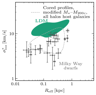
Figure A4: Same as Fig. 4, but for the dashed line we change our free parameters. To avoid crowding the figure, colored regions show 68% of the enclosed population for the LDM case. Our error budget is dominated by the parameters we set free.

Figure A4 shows that the parameters that we set free in our analysis significantly affect our observables. We show the correlation between $\sigma_{\mathrm{los}}^{*}$ and $R_{\mathrm{eff}}$, together with data from classical and SDSS satellites, for the same halo-galaxy connection model and LDM parameters as Fig. 4, but changing our free parameters in the dashed region. To generate the dashed region we set cored profiles for all halo masses, we change the scatter of the stellar mass-halo mass relation by setting $\sigma^{M_{*}}=1.3$ and $\gamma^{M_{*}}=-0.15$, and we set the halo occupation fraction to 1 at all halo masses. Importantly, these parameters are allowed by our analysis. Other parameters are set as in Fig. 4.

We observe that, even if changing our free parameters has a strong impact, the LDM correlation between $\sigma_{\mathrm{los}}^{*}$ and $R_{\mathrm{eff}}$ is still different from CDM. For this correlation to be affected by baryons, baryonic feedback would have to induce increasingly strong cores at lower halo masses, compensating the enhanced LDM mass-concentration relation in Fig. 2. This would be opposite to conventional wisdom, simulation, and observations — lower mass halos tend to be increasingly “cuspy” as they have too few stars to instigate core formation [113, 114, 115].

Appendix B Statistical analysis

We obtain the quantitative conclusions in the main text through a statistical analysis of Milky Way satellite properties. In this Appendix, we describe in detail this analysis.

We fit for the half-light radius, stellar velocity dispersion, and total number of classical and SDSS Milky Way satellites, using the data collected in Ref. [92]. We do not include the Magellanic clouds, Pisces II, and Sagittarius, as baryonic effects and strong tidal stripping could bias our results (the impact of this is minor, as they are a small fraction of our sample). We carry out a frequentist unbinned maximum likelihood,

$$-2\ln\mathcal{L}=-2\sum_{i}\ln\mu(\sigma_{\mathrm{los}}^{*\,\mathrm{obs,}\,i},R_{\mathrm{eff}}^{\mathrm{obs,}\,i})-2\ln\mathcal{P}(N_{\mathrm{obs}})\,.$$ (19)

$\mu(\sigma_{\mathrm{los}}^{*\,\mathrm{obs}},R_{\mathrm{eff}}^{\mathrm{obs}})\,\mathrm{d}\sigma_{\mathrm{los}}^{*\,\mathrm{obs}}\mathrm{d}R_{\mathrm{eff}}^{\mathrm{obs}}$ is the differential probability for a satellite galaxy to have an observed stellar velocity dispersion $\sigma_{\mathrm{los}}^{*\,\mathrm{obs}}$ and half-light radius $R_{\mathrm{eff}}^{\mathrm{obs}}$. $\sigma_{\mathrm{los}}^{*\,\mathrm{obs,}\,i}$ and $R_{\mathrm{eff}}^{\mathrm{obs,}\,i}$ are the observed stellar velocity dispersions and half-light radii, respectively. $\mathcal{P}(N_{\mathrm{obs}})$ is the probability to observe $N_{\mathrm{obs}}$ satellite galaxies, with $N_{\mathrm{obs}}=21$ the number of observed satellites. The first probability is given by

$$\mu(\sigma_{\mathrm{los}}^{*\,\mathrm{obs}},R_{\mathrm{eff}}^{\mathrm{obs}})=\int\mathcal{P}(\sigma_{\mathrm{los}}^{*},R_{\mathrm{eff}},c,M_{*},M)\frac{1}{\sqrt{2\pi}\Delta\sigma}e^{-\frac{(\sigma_{\mathrm{los}}^{*\,\mathrm{obs}}-\sigma_{\mathrm{los}}^{*})^{2}}{2\Delta\sigma^{2}}}\,\frac{1}{\sqrt{2\pi}\Delta R_{\mathrm{eff}}}e^{-\frac{(R_{\mathrm{eff}}^{\mathrm{obs}}-R_{\mathrm{eff}})^{2}}{2\Delta R_{\mathrm{eff}}^{2}}}\mathrm{d}\sigma_{\mathrm{los}}^{*}\,\mathrm{d}R_{\mathrm{eff}}\,\mathrm{d}c\,\mathrm{d}M_{*}\,\mathrm{d}M\,.$$ (20)

$\mathcal{P}(\sigma_{\mathrm{los}}^{*},R_{\mathrm{eff}},c,M_{*},M)\,\mathrm{d}\sigma_{\mathrm{los}}^{*}\,\mathrm{d}R_{\mathrm{eff}}\,\mathrm{d}c\,\mathrm{d}M_{*}\,\mathrm{d}M$ is the differential probability to observe a galaxy with true velocity dispersion $\sigma_{\mathrm{los}}^{*}$, half-light radius $R_{\mathrm{eff}}$, concentration $c$, stellar mass $M_{*}$, and DM halo mass $M$ (for simplicity, in this Appendix we denote $M_{200c}\equiv M$). The two Gaussians are the probabilities to observe a velocity dispersion $\sigma_{\mathrm{los}}^{*\,\mathrm{obs}}$ and half-light radius $R_{\mathrm{eff}}^{\mathrm{obs}}$, given their true values $\sigma_{\mathrm{los}}^{*}$ and $R_{\mathrm{eff}}$ respectively, with $\Delta\sigma$ and $\Delta R_{\mathrm{eff}}$ the observational uncertainties. We assume Gaussian uncertainties for simplicity, as our quantitative statements are only $1\sigma$–$2\sigma$ away from the best fit. We conservatively ignore correlations among $\Delta\sigma$ and $\Delta R_{\mathrm{eff}}$. Should correlations or non-Gaussian uncertainties be provided by observations, they would be straightforward to include.

The expression can be further simplified using conditional probabilities,

$$\begin{split}\mathcal{P}(\sigma_{\mathrm{los}}^{*},R_{\mathrm{eff}},c,M_{*},M)&=\mathcal{P}(\sigma_{\mathrm{los}}^{*},R_{\mathrm{eff}},c,M_{*}|M)\,\mathcal{P}(M)\\ &=\mathcal{P}(\sigma_{\mathrm{los}}^{*},R_{\mathrm{eff}}|c,M_{*},M)\,\mathcal{P}(c,M_{*}|M)\,\mathcal{P}(M)\\ &=\mathcal{P}(\sigma_{\mathrm{los}}^{*}|R_{\mathrm{eff}},c,M_{*},M)\,\mathcal{P}(R_{\mathrm{eff}}|c,M_{*},M)\,\mathcal{P}(c,M_{*}|M)\,\mathcal{P}(M)\,,\end{split}$$ (21)

where

• $\mathcal{P}(M)$ is the product of the subhalo mass function at infall redshift (see Section I in the main text) and the halo occupation fraction. We compute the former with Galacticus following Refs. [43, 48, 51, 52] as described in the main text (Section II.1), and we parametrize the latter as described in the main text (Eq. 13, Section III.1)

  $$\operatorname{hof}(M)=\frac{1+\operatorname{erf}\left(\alpha^{\mathrm{hof}}\log_{10}\left[M/M_{0}^{\mathrm{hof}}\right]\right)}{2}\,,$$ (22)

  with erf the error function, and $\alpha^{\mathrm{hof}}>1$ [33, 64] and $M_{0}^{\mathrm{hof}}$ free parameters. $M$ is the infall mass [135].

• Following the observational results in Ref. [21], we assume that $R_{\mathrm{eff}}$ only depends on stellar mass, i.e., ${\mathcal{P}(R_{\mathrm{eff}}|c,M_{*},M)=\mathcal{P}(R_{\mathrm{eff}}|M_{*})}$. As described in the main text (Eq. 9, Section III.1), we assume a lognormal distribution with median ${\overline{R_{\mathrm{eff}}}=0.021\,M_{*}^{0.239}}$ and scatter of 0.234 dex [21].

  As $R_{\mathrm{eff}}$ only links to halo mass via the stellar mass-halo mass relation, that we set free (see below), observational uncertainties on $\mathcal{P}(R_{\mathrm{eff}}|M_{*})$ do not have a strong impact on our error budget. We also set free the halo occupation fraction, which makes the connection between DM halos and $M_{*}$ even more flexible.

• We assume that $c$ and $M_{*}$ are independent and only related to $M$, $\mathcal{P}(c,M_{*}|M)=\mathcal{P}(c|M)\,\mathcal{P}(M_{*}|M)$. Then,

  • $\mathcal{P}(c|M)$ is, as described in the main text (Section II.1), a lognormal distribution with median computed with Galacticus following Ref. [57] and scatter of 0.16 dex [59].

  • $\mathcal{P}(M_{*}|M)$ is the product of the probability to observe the galaxy given its stellar mass, parametrized by the completeness correction; and the stellar mass-halo mass relation.

    For the completeness correction, we follow Eqs. 14 and 15 in the main text (Section III.1). Although the completeness correction could also depend on surface brightness [100], i.e., on $R_{\mathrm{eff}}$, our large uncertainties on the completeness correction, on the stellar mass-halo mass relation, and on the halo occupation fraction make this correction minor. We include anisotropy-induced scatter as described in the main text (Section IV): we multiply $\mathcal{C}_{\Omega}$ by a free parameter $\sigma_{\mathcal{C}_{\Omega}}$, and we add to the likelihood a Gaussian prior on $\sigma_{\mathcal{C}_{\Omega}}$ centered at 1 and with 19% width [13] (this is a conservative estimate, derived when SDSS was not yet complete). We also include uncertainty in the spatial satellite distribution $n(r)$ due to tidal disruption, by parametrizing $n(r)$ as described in the main text (Eq. 17, Section IV)

    $$n(r)=n_{\mathrm{GK17}}(r)+y_{\mathcal{C}}[n_{\mathrm{NFW}}(r)-n_{\mathrm{GK17}}(r)]\,,$$ (23)

    with $y_{\mathcal{C}}\in[0,1]$ a free parameter that interpolates between an NFW distribution, $n_{\mathrm{NFW}}(r)$, and the tidally disrupted distribution from Ref. [139], $n_{\mathrm{GK17}}(r)$. The latter distribution strongly suppresses the subhalo abundance within the inner $\sim 100\,\mathrm{kpc}$. Enhancements in the number of subhalos within the inner $\sim 50\,\mathrm{kpc}$ due to the recent passage of the Large Magellanic Cloud [62, 63] are smaller than the tidal disruption uncertainty we parametrize by $y_{\mathcal{C}}$.

    For the stellar mass-halo mass relation, we follow Eqs. 10 and 11 in the main text (Section III.1). I.e., we assume it to be a lognormal distribution whose median follows a power law with power $\beta^{M_{*}}$ and normalization $M_{*}(M=1.54\times 10^{12}M_{\odot})=0.0455\,M$ [96], and whose scatter can increase at low mass, [101]

    $$\sigma(M)=\sigma^{M_{*}}+\gamma^{M_{*}}\log_{10}\frac{M}{10^{11}M_{\odot}}\,.$$ (24)

    $\beta^{M_{*}}$, $\sigma^{M_{*}}\in[0,2]$ [101, 64], and $\gamma^{M_{*}}<0$ are free parameters. $M$ is the infall mass [96].

• $\mathcal{P}(\sigma_{\mathrm{los}}^{*}|R_{\mathrm{eff}},c,M_{*},M)=\delta\left(\sigma-\sqrt{\frac{G}{4}\frac{M(<R_{\mathrm{eff}}/0.75)}{R_{\mathrm{eff}}}}\right)$ (Eq. 12 and Section III.1 in the main text), which depends on $M$ and $c$ through the enclosed mass $M(<r)$. For simplicity we ignore scatter, as other mass estimators produce very similar results [16] (see also Fig. A3). As described in the main text (Sections II.1 and III.1), we include baryonic feedback by assuming an NFW profile for $M<M_{\mathrm{thres}}^{\mathrm{core}}$ and a cored profile for $M>M_{\mathrm{thres}}^{\mathrm{core}}$ following Ref. [115] (where the core size depends on the time over which a galaxy has formed stars), with $M_{\mathrm{thres}}^{\mathrm{core}}$ a free parameter.

Since $\mu$ is a differential probability, we numerically normalize it so that $\int\mu(\sigma_{\mathrm{los}}^{*\,\mathrm{obs}},R_{\mathrm{eff}}^{\mathrm{obs}})\,\mathrm{d}\sigma_{\mathrm{los}}^{*\,\mathrm{obs}}\mathrm{d}R_{\mathrm{eff}}^{\mathrm{obs}}=1$.

Finally, we take the probability to observe $N_{\mathrm{obs}}$ satellite galaxies, $\mathcal{P}(N_{\mathrm{obs}})$, to be a negative binomial distribution with intrinsic scatter $\sigma_{I}^{2}=0.18$ [178] and mean

$$N_{\mathrm{expected}}=\int\mathcal{P}(\sigma_{\mathrm{los}}^{*},R_{\mathrm{eff}},c,M_{*},M)\,\mathrm{d}c\,\mathrm{d}M_{*}\,\mathrm{d}M\,\mathrm{d}\sigma_{\mathrm{los}}^{*}\,\mathrm{d}R_{\mathrm{eff}}\,,$$ (25)

i.e., $\mathcal{P}(\sigma_{\mathrm{los}}^{*},R_{\mathrm{eff}},c,M_{*},M)$ is normalized to the expected number of observed galaxies. This integral is dominated by low-mass halos (see Fig. 3), so the effect of not including the Magellanic clouds in our analysis is minor. Changing the Milky Way mass within uncertainties [38] would change $N_{\mathrm{expected}}$ by about 20% [21]. This is smaller than the total scatter of $\mathcal{P}(N_{\mathrm{obs}})$. In addition, our main constraining power on DM properties does not come from the total number of satellites, as that is degenerate with galaxy-halo connection parameters (see Section IV.1 in the main text).

Overall, our likelihood $\mathcal{L}$ depends on 2 parameters describing DM physics, {$n_{\mathrm{cut}}$, $k_{\mathrm{cut}}$}; and 8 parameters modelling galaxy properties and baryonic effects, {$M_{0}^{\mathrm{hof}}$, $\alpha^{\mathrm{hof}}$, $\beta^{M_{*}}$, $\sigma^{M_{*}}$, $\gamma^{M_{*}}$, $M_{\mathrm{thres}}^{\mathrm{core}}$, $\sigma_{\mathcal{C}_{\Omega}}$, $y_{\mathcal{C}}$}. To obtain allowed regions in a subset of parameters, we minimize $-2\ln\mathcal{L}$ over other parameters and assume Wilks’ theorem [179], i.e., that $-2\ln\mathcal{L}$ is distributed following a $\chi^{2}$ distribution with a number of degrees of freedom equal to the number of free parameters. We carry out the integrals with the vegas package [180] and the minimizations with the Py-BOBYQA package [181, 182].

Appendix C Full parameter space scan

In this Appendix, we provide the full results of our statistical analysis.

Table 1 shows our free parameters, the ranges over which we scan in our analysis (in a Bayesian framework, these would correspond to the prior ranges), and the $1\sigma$ preferred ranges after minimizing $-2\ln\mathcal{L}$ over all other parameters. We find that we can constrain many galaxy-halo connection parameters, such as the slope of the stellar mass-halo mass relation, the turning mass of the halo occupation fraction, the halo mass above which baryonic feedback makes DM density profile cored, or the amount of subhalo tidal disruption. Other parameters, such as the slope of the halo occupation fraction or the low-mass growth of stellar mass-halo mass scatter, are more challenging to constrain.

$k_{\mathrm{cut}}/\mathrm{Mpc^{-1}}$ $n_{\mathrm{cut}}$ $M_{0}^{\mathrm{hof}}/M_{\odot}$ $\alpha^{\mathrm{hof}}$ $\beta^{M_{*}}$ $\sigma^{M_{*}}$/dex $\gamma^{M_{*}}$/dex $M_{\mathrm{thres}}^{\mathrm{core}}/M_{\odot}$ $y_{\mathcal{C}}$ $\sigma_{\mathcal{C}_{\Omega}}$ Definition Eq. 1 Eq. 1 Eq. 13 Eq. 13 (10) Eq. 11 Eq. 11 Below Eq. 12 Eq. 17 Below Eq. 17 Value in Fig. 4 8 2.6 $10^{8.35}$ [135, 36] $1.31$ [135, 36] 0.963 [96] 0.15 [96] 0 [96] $10^{9}\,M_{\odot}$ [21] 1 1 Scan range (4, 45) (1, 5) ($10^{7}$, $10^{11}$) (1, 10) [33, 64] (0, 3) (0, 2) [101, 64] (-2, 0) ($10^{7}$, $10^{11}$) (0, 1) (0, 2) $1\sigma$ range (4, 45)^∗ (1, 5)* ($10^{7}$, $10^{7.9}$) (1, 10) (1.0, 1.7) (0, 2)^∗ (-0.7, -0.1)^∗ ($10^{7}$, $10^{8.8}$) (0.3, 1) (0.85, 1.15)

Table 1: Parameters in our analysis. The parameters whose $1\sigma$ range has an ^∗ are strongly correlated with other parameters; if the latter are fixed, the $1\sigma$ range is smaller than the scan range. To generate the theoretical populations in Fig. 4, we use illustrative galaxy-halo connection parameters (see references). Some scan ranges are physics-motivated (see references).

Figure C1 shows the correlations among our free parameters. To better visualize correlations between galaxy-halo connection parameters and enhanced power spectra (i.e., $n_{\mathrm{cut}}>1$), we fix $k_{\mathrm{cut}}=10\,\mathrm{Mpc^{-1}}$. Otherwise, for large enough $k_{\mathrm{cut}}$, any value of $n_{\mathrm{cut}}$ would be degenerate in our halo mass range with a scale-invariant power spectrum (see Figs. 2 and 7). We show the preferred $1\sigma$ and $2\sigma$ regions after minimizing $-2\ln\mathcal{L}$ over all other parameters. We find that, even though there are correlations among galaxy-halo connection parameters — particularly for the stellar mass-halo mass relation —, enhanced power, i.e., a modified $n_{\mathrm{cut}}$, is mostly independent of galaxy-halo connection as described in the main text (Section IV.1). As discussed in Section IV.2, the main correlation of enhanced power is with the halo mass above which baryonic feedback makes DM density profiles cored, i.e., $M_{\mathrm{thres}}^{\mathrm{core}}$.

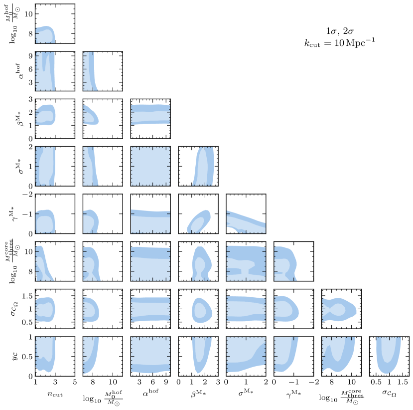
Figure C1: Allowed regions within $1\sigma$ and $2\sigma$ for all parameters in our analysis. For each pair of parameters shown, all other parameters are minimized over in the likelihood. To visualize correlations with our determination of the power spectrum, we fix ${k_{\mathbf{cut}}=10\,\mathrm{Mpc^{-1}}}$. Parameters controlling galaxy-halo connection and baryonic feedback are mostly independent of the DM power spectrum.