Uncovering solutions from data corrupted by systematic errors:
A physics-constrained convolutional neural network approach

Abstract

Information on natural phenomena and engineering systems is typically contained in data. Data can be corrupted by systematic errors in models and experiments. In this paper, we propose a tool to uncover the spatiotemporal solution of the underlying physical system by removing the systematic errors from data. The tool is the physics-constrained convolutional neural network (PC-CNN), which combines information from both the system’s governing equations and data. We focus on fundamental phenomena that are modelled by partial differential equations, such as linear convection, Burgers’ equation, and two-dimensional turbulence. First, we formulate the problem, describe the physics-constrained convolutional neural network, and parameterise the systematic error. Second, we uncover the solutions from data corrupted by large multimodal systematic errors. Third, we perform a parametric study for different systematic errors. We show that the method is robust. Fourth, we analyse the physical properties of the uncovered solutions. We show that the solutions inferred from the PC-CNN are physical, in contrast to the data corrupted by systematic errors that does not fulfil the governing equations. This work opens opportunities for removing epistemic errors from models, and systematic errors from measurements.

1 Introduction

Model estimates and experimental measurements can be affected by systematic errors. Systematic errors can arise for a number of reasons: faulty experimental sensors [1], or low-fidelity numerical methods in which closing nonlinear multiscale equations can add bias, to name a few. The detection and removal of systematic errors has numerous applications, ranging from correcting biased experimental observations, to enhancing results obtained from low-fidelity simulations [2]. In the field of fluid dynamics, experimental measurement of a flow-field is an inherently challenging process. Measurement techniques are often limited given the sensitivity of the flow to immersed sensors and probes, the introduction of which can fundamentally alter the intended behaviour of the system [3]. In many cases, non-intrusive methods such as particle-image-velocimetry are preferred, the results of which provide no guarantee of satisfying the underlying physical laws. Removing systematic errors that are present in these observations would yield the underlying solution of the system. Approaches for recovering a divergence-free field exist, but focus predominantly on filtering out small quantities of stochastic noise [4, 5].

Irrespective of the research domain, a contemporary issue in the field of modelling and simulation is the computational expense of running high-fidelity simulations [6]. In many cases, practitioners rely on lower-fidelity methods, accepting assumptions or approximations, which invoke degrees of model error. We posit that the obtained low-fidelity state can be considered as a corrupted observation because the underlying solution of the system subjected to a form of systematic error. Providing a mapping from the corrupted-state to the underlying solution would allow the inference of high-fidelity results given only low-fidelity data. In practice, we observe that verifying that observations are characteristic of a given system is more straightforward than determining the solution itself. The former requires ensuring that the governing equations are satisfied, whilst the latter requires a method to produce a candidate solution. The overarching goal of this paper is to design a method to remove large-amplitude systematic errors from data to uncover the true solution of the partial differential equation.

Systematic error removal in the literature typically considers the case of aleatoric noise-removal, which is a term attributed to methods that remove small, unbiassed stochastic variations from the underlying solution. This has been achieved through various methods, including filtering methods [7]; proper orthogonal decomposition [8, 9]; and the use of autoencoders [10]. Super-resolution can be considered a form of systematic error removal because its maps low-resolution observations to their equivalent high-resolution representations. In this case, the super-resolution task seeks to introduce additional information, which are not present in the original observation. This resolves the solution at a higher spatial frequency, which is a subtly different task to removing errors from observations. Notable works in this area include methods based on a library of examples [11] and sparse representation in a library [12]. More recent work has employed machine learning methods, including methods based on convolutional neural networks [13], and generative adversarial methods [14].

By exploiting the universal function approximation property of neural networks, it is possible to obtain numerical surrogates for function mappings or operators [e.g., 15, 16]. For a network parameterised by weights, there exists an optimal set of weights that results in the desired mapping; the challenge being to realise these through an optimisation process. This optimisation is formulated as the minimisation of a loss function, the evaluation of which offers a distance metric to the desired solution. When considering forms of structured data, convolutional neural networks excel due to their ability to exploit spatial correlations in the data, which arise from the use of localised kernel operations. In the case of data-driven problems, a typical approach is to minimise a measure of the distance between network realisations and the associated true value. In the absence of knowledge about the true state, it is possible to impose prior knowledge onto the system. For a physical problem, the classical means to accomplish this is through a form of physics-based regularisation, which introduces penalty terms in the loss function to promote physical solutions, i.e., penalising realisations that do not conform to the properties of the system [17]. Inspired by Lagaris et al. [17], Raissi et al. [18] introduced physics-informed neural networks (PINNs), which replace classical numerical solvers with surrogate models. The loss function leverages automatic differentiation to obtain numerical realisations of the gradients of the output (the predicted quantity) with respect to the input, which usually contains the spatiotemporal coordinates.

In this work, we propose a method for removing systematic errors with a physics-constrained machine learning approach. Imposing prior knowledge of the physics allows us to realise a mapping from the corrupted-state to the true-state in the form of a convolutional neural network, as shown in Figure 1. We emphasise that this is not a PINN approach [18] because we do not leverage automatic differentiation to obtain gradients of outputs with respect to inputs to constrain the physics. This network employs a time-batching scheme to effectively compute the time-dependant residuals without resorting to recurrent-based network architectures. Realisations of the network that do not conform to the given partial differential equation are penalised, which ensures that the network learns to produce physical predictions. Ultimately, this allows the effective removal of additive systematic error from data.

In section §2, we formulate the problem of the systematic error removal. An overview of convolutional neural networks is provided in section §3, which highlights how we can exploit the spatial invariance and describes the architecture employed for the systematic error removal task. We detail the methodology in section §3.1, which provides justifications for the design of the loss function, before showcasing results in section §5. We provide a form of parameterised systematic error using a multimodal function [19], which allows us to explore the effect of high wavenumbers and magnitudes of the systematic error. Results are obtained from three systems of increasing physical complexity: linear convection-diffusion, nonlinear convection-diffusion, and a two-dimensional turbulent flow. We further analyse results for the two-dimensional turbulent flow case, investigating the physical coherence of network predictions. Section §7 ends the paper.

2 Problem formulation

We consider physical systems that can be modelled by partial differential equations (PDEs). Upon suitable spatial discretisation, a PDE with boundary conditions is viewed as a dynamical system in the form of

$$\mathcal{R}({\bm{u}};\lambda)\equiv\partial_{t}{\bm{u}}-\mathcal{N}({\bm{u}};\lambda),$$ (1)

where ${\bm{x}}\in\Omega\subset\mathbb{R}^{n}$ denotes the spatial location; $t\in[0,T]\subset\mathbb{R}_{\geq 0}$ is the time; ${\bm{u}}:\Omega\times[0,T]\rightarrow\mathbb{R}^{m}$ is the state; $\lambda$ are physical parameters of the system; $\mathcal{N}$ is a sufficiently smooth differential operator; $\mathcal{R}$ is the residual; and $\partial_{t}$ is the partial derivative with respect to time. A solution of the PDE ${\bm{u}}^{\ast}$ is the function that makes the residual vanish, i.e., $\mathcal{R}({\bm{u}}^{\ast};\lambda)=0$.

We consider that the observations on the system’s state, ${\bm{\zeta}}({\bm{x}},t)$, are corrupted by an additive systematic error

$$\bm{\zeta}(\bm{x},t)={\bm{u}}^{\ast}(\bm{x},t)+{\bm{\phi}}({\bm{x}}),$$ (2)

where ${\bm{\phi}}$ is the stationary systematic error, which is spatially varying. For example, additive systematic errors can be caused by miscalibrated sensors [1], or modelling assumptions [20]. The quantity in Eq. (2) constitutes the corrupted dataset, which fulfils the inequality

$$\mathcal{R}({\bm{\zeta}}({\bm{x}},t);\lambda)\neq 0.$$ (3)

Given the corrupted state, ${\bm{\zeta}}$, we wish to uncover the underlying solution to the governing equations, ${\bm{u}}^{\ast}$, which is referred to as the true state. Mathematically, we need to compute a mapping, ${\bm{\eta_{\theta}}}$ such that

$${\bm{\eta_{\theta}}}:{\bm{\zeta}}({\bm{\Omega}}_{g},t)\mapsto{\bm{u}}^{\ast}({\bm{\Omega}}_{g},t),$$ (4)

where the domain $\Omega$ is discretised on a grid ${\bm{\Omega}}_{g}\subset\mathbb{R}^{N^{n}}$, which is uniform and structured in this study. We assume the mapping ${\bm{\eta_{\theta}}}$ to be a parametric function, which depends on the parameters ${\bm{\theta}}$ that need to be found. In section §3, we describe the parametric function that we employ in this study. Figure 1 provides an overview of the systematic error removal problem, which is applied to a turbulent flow. The corrupted field ${\bm{\zeta}}(\bm{\Omega_{g}},t)$ is passed as input to the appropriately trained model ${\bm{\eta_{\theta}}}$, which allows us to uncover the underlying solution ${\bm{u}^{\ast}}$ to the partial differential equation, and, as a byproduct, the additive systematic error ${\bm{\phi}}$.

The linear vs. nonlinear nature of the partial differential equations has a computational implication. For a linear partial differential equation, the residual is an explicit function of the systematic error, i.e., $\mathcal{R}({{\bm{\zeta}}({\bm{x}},t)};\lambda)=\mathcal{R}({{\bm{\phi}}({\bm{x}},t)};\lambda)$. This does not hold true for nonlinear systems, which makes the problem of removing systematic error more challenging. This is discussed in section §5.

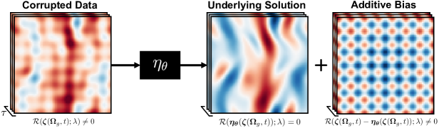
Figure 1: Removal of systematic error from data. The model ${\bm{\eta_{\theta}}}$ is responsible for recovering the underlying solution, ${\bm{u}}^{\ast}({\bm{\Omega}}_{g},t)$, from the corrupted data, ${\bm{\zeta}}(\bm{\Omega}_{g},t)$. The systematic error, ${\bm{\phi}}({\bm{x}})$, is the difference between the corrupted data and the underlying solution.

3 The Physics-constrained convolutional neural network

We propose the physics-constrained convolutional neural network (PC-CNN) for uncovering solutions of PDEs from corrupted data. Convolutional neural networks are suitable tools for structured data, which ensure shift invariance [21, 22]. When working with data from partial differential equations, the spatial structure is physically correlated with respect the characteristic spatial scale of the problem, for example, correlation lengths in turbulent flows, diffusive spatio-temporal scales in convection, among others [23]. By leveraging an architectural paradigm that exploits these spatial structures, we propose parameterised models that, when appropriately trained and tuned, can generalise to unseen data [24, 25]. We provide a brief summary of convolutional neural networks and refer the reader to [26] for a pedagogical explanation. A convolutional layer is responsible for the discrete mapping

$$\kappa:({\bm{w}},{\bm{b}},{\bm{x}})\mapsto{\bm{x}}\ast{\bm{w}}+{\bm{b}},$$ (5)

where ${\bm{w}}\in\mathbb{R}^{k^{d}\times c_{o}}$ represents a trainable kernel; ${\bm{b}}\in\mathbb{R}^{c_{o}}$ is an additive bias; $\ast$ the convolution operation; and $\bm{x}\in\mathbb{R}^{m^{d}\times c_{i}}$ is the input data. The number of parameters in the network is proportional to the dimensionality of the kernels, whose spatial extent is determined by $k$, while the number of filters, or channels, is given by $c_{o}$. The dimensionality of the input is independent of the kernel and bias, with $c_{i}$ determining the number of input channels. The trainable kernel $\kappa$ operates locally around each pixel, which leverages information from the surrounding grid cells. As such, convolutional layers are an excellent choice for learning and exploiting local spatial correlations [21, 27, 28]. Each channel in the kernel is responsible for extracting different features present in the input data. This determines the degree to which an arbitrary function can be learned, as per the universal approximation theorem [15]. A convolutional neural network is an architecture that leverages multiple convolutions, which can be viewed as a composition of multiple layers where $Q$ is the number of layers

$${\bm{\eta_{\theta}}}={\bm{\eta}}^{Q}_{\bm{\theta}_{Q}}\circ\cdots\circ h({\bm{\eta}}^{1}_{\bm{\theta}_{1}})\circ h({\bm{\eta}}^{0}_{\bm{\theta}_{0}}).$$ (6)

In the most basic form, each layer ${\bm{\eta}}_{\theta_{i}}^{i}$ is a convolution $\kappa$ followed by an element-wise nonlinear activation function $h$. In the absence of nonlinearities, a network is capable only of learning a linear transformation, which restricts the function approximation space [29]. The introduction of these nonlinear activations is a key ingredient to the expressivity of the network. The final layer ${\bm{\eta}}_{\bm{\theta}_{Q}}^{Q}$ is exempt from activation as this limits the expressive power of the output. There are a number of modifications that can be made to each layer, we refer the reader to [30] for a more general treatment of the topic. As the filter is convolved over each discrete pixel, the operation on large spatial domains may become computationally expensive due to the $\mathcal{O}(k^{2})$ scaling. To mitigate the increased computational expense, we choose a kernel size $k=3$ for each convolutional layer, which is a common choice for CNN architectures [30].

The basic architecture is extended through the use of pooling and upsampling layers to vary the spatial dimensionality of the input to sequential convolutional layers. In this work, we employ mean pooling and bilinear upsampling with a kernel size of $k=2$ in each case. Varying the dimensionality of the input to the layers aids with feature extraction and provides another means to reduce the computational expense of the network – each filter $\kappa$ is convolved over a smaller spatial domain. Figure 2 depicts the architecture used for the systematic error removal task, which highlights the operations employed with the dimensionality at each layer. The corrupted observations ${\bm{\zeta}}({\bm{\Omega}}_{g},t)$ are passed as input to the network, with the outputs estimating the predicted true-state, ${\bm{\eta_{\theta}}}({\bm{\zeta}}({\bm{\Omega}}_{g},t))$.

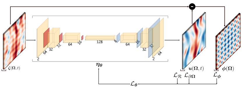
Figure 2: Diagram of network architecture and training pipeline. In the network architecture ${\bm{\eta_{\theta}}}$: yellow layers denote convolution operations; red layers denote mean-pooling; blue layers denote bi-linear interpolation. Composite losses $\mathcal{L}_{\mathcal{R}},\mathcal{L}_{\partial{\bm{\Omega}}},\mathcal{L}_{\bm{\phi}}$ are computed on the output field and inferred systematic error. These are then combined to compute the training loss $\mathcal{L}_{\bm{\theta}}$, which is used to update weights ${\bm{\theta}}$ of the network. We provide an in-depth explanation of these losses in section §3.1.

3.1 Constraining the physics

The convolutional neural network, ${\bm{\eta_{\theta}}}$, defines a nonlinear parametric mapping, whose parameters, ${\bm{\theta}}$, are found by training. The information constrained in the training originates from two sources. First the data, which may be corrupted; and second, the prior knowledge on the physical system, which is encoded in partial differential equations. The training is an minimisation problem of a cost functional $\mathcal{L}_{\bm{\theta}}$, which reads

$${\bm{\theta}}^{*} =\operatorname*{argmin}_{\bm{\theta}}\mathcal{L}_{\bm{\theta}},$$ (7)

$$\mathcal{L}_{\bm{\theta}} =\mathcal{L}_{\mathcal{R}}+\alpha\left(\mathcal{L}_{\partial{\bm{\Omega}}}+\mathcal{L}_{\bm{\phi}}\right),$$

where $\alpha$ is a fixed, empirical weighting factor, which determines the relative importance of the loss terms. Given corrupted-data ${\bm{\zeta}}({\bm{\Omega}_{g}},t)$ at times $t\in\mathcal{T}\subseteq[0,T]$, we define each of the loss terms in Eq. 7 as

$$\mathcal{L}_{\mathcal{R}} =\frac{1}{N_{\mathcal{T}}}\sum_{t\in\mathcal{T}}\big{\lVert}\mathcal{R}\big{(}{\bm{\eta_{\theta}}}({\bm{\zeta}}({\bm{\Omega}}_{g},t));\lambda\big{)}\big{\rVert}_{{\bm{\Omega}}_{g}}^{2},$$ (8)

$$\mathcal{L}_{\partial{\bm{\Omega}}} =\frac{1}{N_{\mathcal{T}}}\sum_{t\in\mathcal{T}}\big{\lVert}{\bm{\eta_{\theta}}}({\bm{\zeta}}(\partial{\bm{\Omega}}_{g},t))-{\bm{u}}(\partial{\bm{\Omega}}_{g},t)\big{\rVert}_{\partial{\bm{\Omega}}_{g}}^{2},$$ (9)

$$\mathcal{L}_{\bm{\phi}} =\frac{1}{N_{\mathcal{T}}}\sum_{t\in\mathcal{T}}\big{\lVert}\partial_{t}\big{[}{\bm{\zeta}}({\bm{\Omega}}_{g},t)-{\bm{\eta_{\theta}}}({\bm{\zeta}}({\bm{\Omega}}_{g},t))\big{]}\big{\rVert}_{{\bm{\Omega}}_{g}}^{2},$$ (10)

where $N_{\mathcal{T}}$ is the number of time steps; $\partial{\bm{\Omega}}_{g}$ denotes boundary points of the grid, and $\lVert\mathrel{\;\cdot\;}\rVert_{{\bm{\Omega}}_{g}}$ is the $\ell^{2}$-norm over the given domain. The terms $\mathcal{L}_{\mathcal{R}},\mathcal{L}_{\partial{\bm{\Omega}}},\mathcal{L}_{\bm{\phi}}$ denote the residual loss, boundary loss, and systematic error loss, respectively.

In order to find an optimal set of parameters ${\bm{\theta}}^{*}$, the loss is designed to penalise, or regularise, predictions, which do not conform to the desired output. We impose prior-knowledge of the dynamical system using the residual-based loss $\mathcal{L}_{\mathcal{R}}$, promoting parameters that yield predictions that conform to the governing equations. Successful minimisation of the residual-based loss ensures that network realisations satisfy the residual of the system, as shown in Eq. (1). The magnitude of parameter updates $\nicefrac{{\partial\mathcal{L}_{\bm{\theta}}}}{{\partial{\bm{\theta}}}}$ is proportional to the magnitude of the loss, which ensures large violations of the residual are heavily regularised.

The residual-based loss alone is insufficient for obtaining the desired mapping. In the absence of collocation points the mapping ${\bm{\eta_{\theta}}}$ provides a non-unique mapping: any prediction that satisfies the governing equations is valid. To avoid this we impose knowledge of the ground truth solution at select collocation points, chosen to lie on the boundaries of the domain $\partial{\bm{\Omega}}$. The data-driven boundary loss $\mathcal{L}_{\partial{\bm{\Omega}}}$ is designed to minimise the error between predictions and measurements at the chosen collocation points. This has the effect of restricting the function approximation space to provide a unique mapping and ensuring that the predictions satisfy the observations.

Inclusion of the systematic-error-based loss $\mathcal{L}_{\bm{\phi}}$ embeds our assumption of stationary systematic error ${\bm{\phi}}={\bm{\phi}}(x)$. Penalising network realisations that do not provide a unique systematic error helps stabilise training and drive predictions away from trivial solutions, such as the stationary solution ${\bm{u}}({\bm{\Omega}}_{g},t)=0$. Consequently, this eliminates challenging local minima in the loss surface, which improves convergence of the optimisation approach shown in Eq. (7).

3.2 Time-batching

The computation of the residual of partial differential equations in time is inherently temporal in nature, as can be seen in Eq. 1. Convolutional neural networks do not consider the sequentiality of the data in their architecture. In this paper, we propose time-batching the data to compute the time derivative $\partial_{t}{\bm{u}}$, which is necessary in the residual computation. We consider each sample passed to the network to constitute a window of $\tau$ sequential timesteps. This allows both computing predictions in parallel and sharing weights, which decreases the computational cost of the problem. Employing a time windowing approach provides a number of benefits, i.e., it allows us to process non-contiguous elements of the timeseries, and sample different points in the temporal domain. We provide an explicit formulation for the residual-based loss

$$\mathcal{L}_{\mathcal{R}}=\frac{1}{\tau N_{\mathcal{T}}}\sum_{t\in\mathcal{T}}\sum_{n=0}^{\tau}\big{\lVert}\partial_{t}{\bm{\eta_{\theta}}}({\bm{\Omega}}_{g},t+n\Delta t))-\mathcal{N}({\bm{\eta_{\theta}}}({\bm{\zeta}}({\bm{\Omega}}_{g},t+n\Delta t));\lambda)\big{\rVert}_{{\bm{\Omega}}_{g}}^{2},$$ (11)

in which the time-derivative is computed using the explicit forward-Euler method over predictions at subsequent timesteps, and the differential operator is evaluated at each timestep. In so doing, we are able to obtain the residual for the predictions in a temporally local sense; rather than computing the residual across the entire time-domain, we are able to compute the residual over each time window. This reduces the computational cost and increases the number of independent batches provided to the network.

We augment the other loss terms to operate in the same manner, operating over the time window as well as the conventional batch dimension. While the time-independent boundary loss $\mathcal{L}_{\partial{\bm{\Omega}}}$ need not leverage the connection between adjacent timesteps, the systematic error loss $\mathcal{L}_{\bm{\phi}}$ computes the time-derivative in the same manner - evaluating the forward-Euler method between consecutive timesteps.

3.2.1 Choice of the time window

The choice of the time window $\tau$ is important. For a fixed quantity of training data, we need to consider the trade-off between computing the residual over longer time windows, and sampling a larger number of windows from within the time domain. If we consider $N=\tau N_{\mathcal{T}}$ training samples, a larger value of $\tau$ corresponds to fewer time windows. Limiting the number of time windows used for training has an adverse effect on the ability of the model to generalise; the information content of contiguous timesteps is scarcer than taking timesteps uniformly across the time domain. A further consideration is that, although evaluating the residual across large time windows promotes numerical stability, this smooths the gradients computed in backpropagation, and makes the model more difficult to train, especially in the case of chaotic systems. Empirically, we choose $\tau=2$, the minimum window size feasible for computing the residual-based loss $\mathcal{L}_{\mathcal{R}}$. We find that this is sufficient for training the network whilst simultaneously maximising the number of independent samples used for training. To avoid duplication of data in the training set, we ensure that all samples are at least $\tau$ timesteps apart so that independent time windows are guaranteed to not contain any overlaps.

4 Data generation

A high-fidelity numerical solver provides the datasets used throughout this paper. We utilise a differentiable pseudospectral spatial discretisation to solve the partial differential equations of this paper [31]. The solution is computed on on the spectral grid ${\bm{\hat{\Omega}}}_{k}\in\mathbb{Z}^{K^{n}}$. This spectral discretisation spans the spatial domain ${\Omega}\in[0,2\pi)\subset\mathbb{R}^{2}$, enforcing periodic boundary conditions on $\partial\Omega$. A solution is produced by time-integration of the dynamical system with the explicit forward-Euler scheme, in which we choose the timestep $\Delta t$ to satisfy the Courant-Friedrichs-Lewy (CFL) condition [32]. The initial conditions in each case are generated using the equation

$${\bm{u}}^{\ast}({\bm{\hat{\Omega}}}_{k},0)=\frac{\iota e^{2\pi i{\bm{\epsilon}}}}{\sigma\sqrt{2\pi}}e^{-\frac{1}{2}\left(\frac{\lvert{\bm{\hat{\Omega}}}_{k}\rvert}{\sigma}\right)^{2}}\qquad\text{with}\quad{\bm{\epsilon}}_{i}\sim N(0,1),$$ (12)

where $\iota$ denotes the magnitude; $\sigma$ denotes the standard deviation; and ${\bm{\epsilon}}_{i}$ is a sample from a unit normal distribution. Equation 12 produces a pseudo-random field scaled by the wavenumber ${\bm{\hat{\Omega}}}_{k}$, which ensures that the resultant field has spatial structures of varying lengthscale. We take $\iota=10,\sigma=1.2$ for all simulations in order to provide an initial condition, which provides numerical stability.

As a consequence of the Nyquist-Shannon sampling criterion [32], the resolution of the spectral grid ${\bm{\hat{\Omega}}}_{k}\in\mathbb{Z}^{K^{n}}$ places a lower bound on the spatial resolution. For a signal containing a maximal frequency $\omega_{\text{max}}$, the sampling frequency $\omega_{s}$ must satisfy the condition $\omega_{\text{max}}<\nicefrac{{\omega_{s}}}{{2}}$, therefore, we ensure that the spectral resolution satisfies $K<\nicefrac{{N}}{{2}}$. Violation of this condition induces spectral aliasing, in which energy content from frequencies exceeding the Nyquist limit $\nicefrac{{\omega_{s}}}{{2}}$ is fed back to the low frequencies, which amplifies energy content unphysically. To prevent aliasing, we employ a spectral grid ${\bm{\hat{\Omega}}}_{k}\in\mathbb{Z}^{32\times 32}$, sampling on the physical grid ${\bm{\Omega}_{g}}\in\mathbb{R}^{64\times 64}$. Approaching the Nyquist limit allows us to resolve the smallest turbulent structures possible without introducing spectral aliasing.

The pseudospectral discretisation [31] provides an efficient means to compute the differential operator $\mathcal{N}$. This allows us to accurately evaluate the residual-based loss $\mathcal{L}_{\mathcal{R}}$ in the Fourier domain

$$\mathcal{L}_{\mathcal{R}}=\frac{1}{\tau N_{\mathcal{T}}}\sum_{t\in\mathcal{T}}\sum_{n=0}^{\tau}\lVert\partial_{t}\hat{{\bm{\eta_{\theta}}}}({\bm{\zeta}}({\bm{\Omega}}_{g},t+n\Delta t))-\hat{\mathcal{N}}(\hat{{\bm{\eta_{\theta}}}}({\bm{\zeta}}({\bm{\Omega}}_{g},t+n\Delta t)))\rVert_{\hat{\bm{\Omega}}_{k}}^{2},$$ (13)

in which $\hat{{\bm{\eta_{\theta}}}}=\mathcal{F}\circ{\bm{\eta_{\theta}}}$ where $\mathcal{F}$ is the Fourier operator, and $\hat{\mathcal{N}}$ denotes the Fourier-transformed differential operator. Computing the loss $\mathcal{L}_{\mathcal{R}}$ in the Fourier domain provides two advantages: (i) periodic boundary conditions are enforced automatically, which enables us to embed prior knowledge in the loss calculations; and (ii) gradient calculations have spectral accuracy [32]. In contrast, a conventional finite differences approach requires a computational stencil, the spatial extent of which places an error bound on the gradient computation. This error bound itself a function of the spatial resolution of the field.

5 Results

In this section, we first introduce the mathematical parameterisation of the systematic error and provide an overview of the numerical details, data and performance metrics used in the study. Second, we demonstrate the ability of the model to recover the underlying solution for three partial differential equations, and analyse the robustness and accuracy. We consider three partial differential equations of increasing complexity: the linear convection-diffusion, nonlinear convection-diffusion (Burgers’ equation [33, 34]), and two-dimensional turbulent Navier-Stokes equations (the Kolmogorov flow [35]). Finally, we analyse the physical consistency of physics-constrained convolutional neural network (PC-CNN) predictions for the two-dimensional turbulent flow. These analyses show the method, up to challenging partial differential equations exhibiting nonlinear, chaotic behaviour.

5.1 Parameterisation of the systematic error

The systematic error is defined with the modified Rastrigin parameterisation [19], which is commonly used in non-convex optimization benchmarks. The Rastrigin parameterisation by both frequency and magnitude allows us to assess the performance for a range of corrupted fields, which have multi-modal features. Multi-modality is a significant challenge for uncovering the solutions of partial differential equations from corrupted data. We parameterise the systematic error as

$${\bm{\phi}}({\bm{x}};\mathcal{M},k_{\phi},u_{\text{max}})=\frac{\mathcal{M}u_{\text{max}}}{2\pi^{2}+40}\left(20+\sum_{i=1}^{2}\left[({\bm{x}}_{i}-\pi)^{2}-10\cos(k_{\phi}({\bm{x}}_{i}-\pi))\right]\right)$$ (14)

where $\mathcal{M}$ is the relative magnitude of systematic error; $u_{\text{max}}$ is the maximum velocity observed in the flow; and $k_{\phi}$ is the Rastrigin wavenumber of the systematic error. Parameterising the systematic error in this manner allows us to evaluate the performance of the methodology with respect to the magnitude and modality of the error.

5.2 Numerical details, data, and performance metrics

We uncover the solutions of partial differential equations from corrupted data for three physical systems of increasing complexity. Each systems is solved via the pseudospectral discretisation as described in section §4, producing a solution by time-integration using the Euler-forward method with timestep of $\Delta t=5\times 10^{-3}$. The time step is chosen to satisfy of the Courant-Friedrichs-Lewy (CFL) condition to promote numerical stability. The model training is performed with $1024$ training samples and $256$ validation samples, which are pseudo-randomly selected from the time-domain of the solution. The adam optimiser is employed [36] with a learning rate of $3\times 10^{-4}$. The weighting factor for the loss $\mathcal{L}_{\bm{\theta}}$ (Eq. 7) is $\alpha=10^{3}$, which is empirically determines to provide stable training. Each model is trained for a total of $10^{4}$ epochs, which is chosen to provide sufficient convergence. The accuracy of prediction is quantified by the relative error on the validation dataset

$$e=\sqrt{\frac{\sum_{t\in\mathcal{T}}\lVert{\bm{u}}^{\ast}(\bm{\Omega_{g}},t)-{\bm{\eta_{\theta}}}({\bm{\zeta}}(\bm{\Omega_{g}},t))\rVert_{\bm{\Omega_{g}}}^{2}}{\sum_{t\in\mathcal{T}}\lVert{\bm{u}}^{\ast}(\bm{\Omega_{g}},t)\rVert_{\bm{\Omega_{g}}}^{2}}}.$$ (15)

This metric takes the magnitude of the solution into account, which allows the results from different systems to be compared. All experiments are run on a single Quadro RTX 8000 GPU.

5.3 Uncovering solutions from corrupted data

In this section, we uncover solutions from corrupted data with testcases on the linear convection-diffusion equation, the Burgers’ equation, and the two-dimensional turbulent Navier-Stokes flow.

5.3.1 The linear convection-diffusion equation

The linear convection-diffusion equation is used to describe a variety of physical phenomena [37]. The equation is defined as

$$\partial_{t}{\bm{u}}+{\bm{c}}\cdot\nabla{\bm{u}}={\nu}\Delta{\bm{u}},$$ (16)

where $\nabla$ is the nabla operator; $\Delta$ is the Laplacian operator; ${\bm{c}}\equiv(c,c)$, where $c$ is the convective coefficient; and ${\nu}$ is the diffusion coefficient. The dissipative nature of the flow is further exacerbated by the presence of periodic boundary conditions. The flow energy is subject to rapid decay because the solution quickly converge towards a fixed-point solution at ${\bm{u}}^{\ast}(\bm{\Omega_{g}},t)=0$. In the presence of the fixed-point solution, we observe ${\bm{\zeta}}({\bm{\Omega}}_{g},t)={\bm{\phi}}({\bm{\Omega}_{g}})$, which is a trivial case for identification and removal of the systematic error. In order to avoid rapid convergence to the fixed-point solution, we take ${c}=1.0,{\nu}=\nicefrac{{1}}{{500}}$ as the coefficients, producing a convective-dominant solution.

A snapshot of the results for $k_{\phi}=3,\mathcal{M}=0.5$ is shown in Figure 3(a). There is a marked difference between the corrupted observations ${\bm{\zeta}}({\bm{\Omega}}_{g},t)$ in panel (i) and the underlying solution ${\bm{u}}^{\ast}({\bm{\Omega}}_{g},t)$ in panel (ii), most notably in the magnitude of the field. Network predictions ${\bm{\eta_{\theta}}}({\bm{\zeta}}({\bm{\Omega}}_{g},t))$ in panel (iii) uncover the underlying solution to the partial differential equation with a relative error of $e=6.612\times 10^{-2}$ on the validation set.

5.3.2 Nonlinear convection-diffusion equation

The nonlinear convection-diffusion equation, also known as Burgers’ equation [34], is

$$\partial_{t}{\bm{u}}+\left({\bm{u}}\cdot{\nabla}\right){\bm{u}}={\nu}\Delta{\bm{u}},$$ (17)

where the nonlinearity is in the convective term $\left({\bm{u}}\cdot{\nabla}\right){\bm{u}}$, the cause of turbulence in the Navier-Stokes equations. The nonlinear convective term provides a further challenge: below a certain threshold, the velocity interactions lead to further energy decay. The kinematic viscosity is set to ${\nu}=\nicefrac{{1}}{{500}}$, which produces a convective-dominant solution by time integration.

In contrast to the linear convection-diffusion system, the relationship between the dynamics of corrupted-state and the true-state is more challenging. The introduction of nonlinearities in the differential operator revoke the linear relationship between the systematic error and observed state, i.e., $\mathcal{R}({{\bm{\zeta}}({\bm{x}},t)};\lambda)\neq\mathcal{R}({{\bm{\phi}}({\bm{x}},t)};\lambda)$ as discussed in section §2. Consequently, this increases the complexity of the residual-based loss term $\mathcal{L}_{\mathcal{R}}$. Figure 3(b) shows a snapshot of results for $k_{\phi}=5,\mathcal{M}=0.5$. The underlying solution ${\bm{u}}^{\ast}({\bm{\Omega}}_{g},t)$ of the partial differential equation contains high-frequency spatial structures, shown in panel (ii), which are less prominent in the corrupted data ${\bm{\zeta}}({\bm{\Omega}}_{g},t)$, shown in panel (i). Despite the introduction of a nonlinear differential operator, we demonstrate that the network retains the ability to recover the underlying solution, with no notable difference in the structure between the predicted and ground-truth fields, shown in panels (iv) and (ii), respectively. The relative error on the validation set is $e=6.791\times 10^{-2}$.

5.3.3 Two-dimensional turbulent flow

We consider a chaotic flow, which is governed by the incompressible Navier-Stokes equations evaluated on a two-dimensional domain with periodic boundary conditions and a periodic forcing term. This flow is also knows as the Kolmogorov flow [35]. The equations are expressions of the mass and momentum conservation, respectively

$${\nabla}\cdot{\bm{u}} =0,$$ (18)

$$\partial_{t}{\bm{u}}+\left({\bm{u}}\cdot{\nabla}\right){\bm{u}} =-{\nabla}p+{\nu}\Delta{\bm{u}}+{\bm{g}}.$$

where $p$ is the scalar pressure field; ${\nu}$ is the kinematic viscosity; and ${\bm{g}}$ is a body forcing, which enables the dynamics to be sustained by ensuring that the flow energy does not dissipate at regime. The flow density is constant and assumed to be unity.

The use of a pseudospectral discretisation allows us to eliminate the pressure term and handle the continuity constraint implicitly, as shown in the spectral representation of the two-dimensional turbulent flow

$$\left(\frac{d}{dt}+\nu\lvert\bm{k}\rvert^{2}\right)\bm{\hat{u}}_{k} =\bm{\hat{f}}_{k}-\bm{k}\frac{\bm{k}\cdot\bm{\hat{f}}_{k}}{\lvert\bm{k}\rvert^{2}}+\bm{\hat{g}}_{k}\qquad\text{with}\quad\bm{\hat{f}}_{k}=-\left(\widehat{\bm{u}\cdot\nabla\bm{u}}\right)_{k},$$ (19)

$$\mathcal{R}(\bm{\hat{u}}_{k};\lambda) =\left(\frac{d}{dt}+\nu\lvert\bm{k}\rvert^{2}\right)\bm{\hat{u}}_{k}-\bm{\hat{f}}_{k}+\bm{k}\frac{\bm{k}\cdot\bm{\hat{f}}_{k}}{\lvert\bm{k}\rvert^{2}}-\bm{\hat{g}}_{k},$$

where nonlinear terms are handled in the pseudospectral sense, employing the standard $\nicefrac{{2}}{{3}}$ de-aliasing rule to avoid un-physical culmination of energy at the high frequencies [32]. As a result of implicit handling of the continuity constraint, we can use the residual-based loss as prescribed without imposing any further constraints for mass conservation.

The presence of the pressure gradient, ${\bm{\nabla}}p$, and forcing term, ${\bm{g}}={\bm{g}}({\bm{x}})$ induce chaotic dynamics in the form of turbulence for $Re=\nicefrac{{1}}{{\nu}}>40$. We take ${\nu}=\nicefrac{{1}}{{42}}$ to ensure chaotic dynamics, imposing constant periodic forcing with ${\bm{g}}(\bm{x})=(\sin{(4\bm{x_{2}}),0})$. In order to remove the transient and focus on a statistically stationary regime, the transient up to $T_{t}=180.0$ is not recorded in the data.

A snapshot for the two-dimensional turbulent flow case is shown in Figure 3(c) for $k_{\phi}=7,\mathcal{M}=0.5$. The corrupted field ${\bm{\zeta}}({\bm{\Omega}}_{g},t)$ as shown in panel (i) contains prominent, high-frequency spatial structures not present in the underlying solution ${\bm{u}}^{\ast}({\bm{\Omega}}_{g},t)$ shown in panel (ii). The corrupted field bares little resemblance to the true solution. In spite of the chaotic dynamics of the system, we demonstrate that the network ${\bm{\eta_{\theta}}}({\bm{\zeta}}({\bm{\Omega}}_{g},t))$ shown in panel (iv) successfully removes the systematic error. The relative error on the validation set is $e=2.044\times 10^{-2}$.

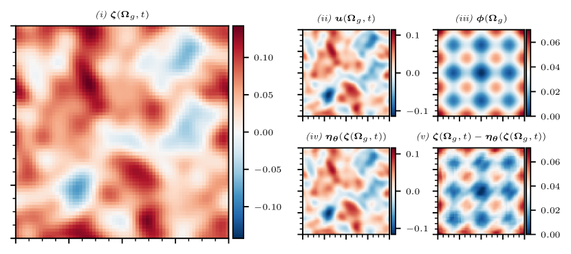
(a) Linear convection-diffusion case $[k_{\phi}=3,\mathcal{M}=0.5]$.

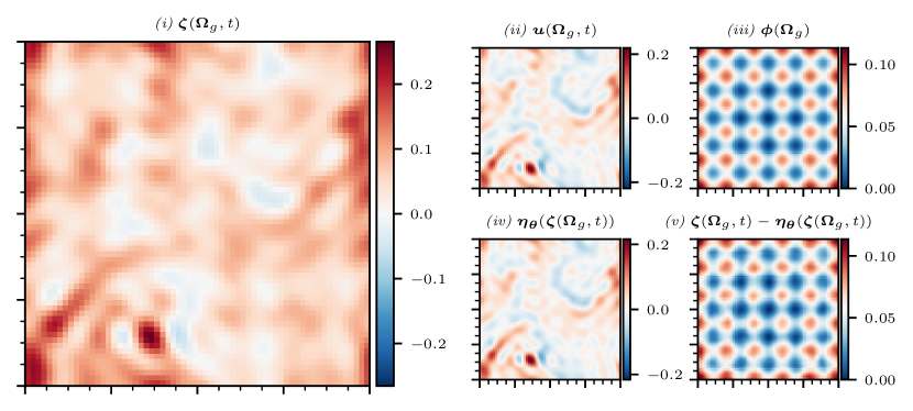
(b) Nonlinear convection-diffusion case $[k_{\phi}=5,\mathcal{M}=0.5]$.

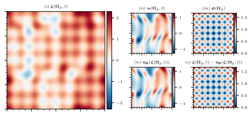
(c) Two-dimensional turbulent flow case $[k_{\phi}=7,\mathcal{M}=0.5]$.

Figure 3: Snapshots of uncovered solutions from corrupted data. Panel (i) shows the corrupted field; (ii) shows the ground-truth solution; (iii) shows the true systematic error; and (iv) shows the network predictions; (v) shows the predicted systematic error.

5.4 Robustness

In this section, we analyse the robustness of the methodology to systematic errors of varying modality and magnitude. The systematic error, ${\bm{\phi}}(\bm{\Omega}_{g})$, is varied for a range of Rastrigin wavenumbers $k_{\phi}$ and relative magnitudes $\mathcal{M}$. These parameter ranges allow us to assess the degree to which the underlying solution of a partial differential equation can be recovered when subjected to spatially varying systematic error with different degrees of multi-modality and magnitudes. To this end, we propose two parametric studies for each partial differential equation

$$\begin{aligned} &\mathit{(i)}\\ &\mathit{(ii)}\end{aligned}\quad\begin{aligned} &\mathcal{M}=0.5,\\ &k_{\phi}=3,\end{aligned}\quad\begin{aligned} k_{\phi}&\in\{1,3,5,7,9\};\\ \mathcal{M}&\in\{0.01,0.1,0.25,0.5,1.0\}.\end{aligned}$$

In the first case, we fix the relative magnitude and vary the Rastrigin wavenumber, whereas in the second case we fix the Rastrigin wavenumber and vary the relative magnitude. For each case, we compute the relative error, $e$, between the predicted solution ${\bm{\eta_{\theta}}}({\bm{\zeta}}(\bm{\Omega_{g}},t))$ and the true solution ${\bm{u}}^{\ast}(\bm{\Omega}_{g},t)$, as defined in Eq. (15). We show the mean error for five repeats of each experiment to ensure results are representative of the true performance. Empirically, we find that performance is robust to pseudo-random initialisation of network parameters with standard deviation of $\mathcal{O}(10^{-4})$.

Computational resource is fixed for each run, which employs the same experimental setup described in section §5.2. Whilst the optimal hyperparameters are likely to vary on a case-by-case basis, providing a common baseline allows for explicit comparison between cases. Assessing results using the same hyperparameters for the three partial differential equations allows us to explore the robustness of the methodology.

In the case of systematic error removal for the linear convection-diffusion problem, shown in Figure 4(a), we demonstrate that the relative error is largely independent of the form of parameterised systematic error. The relative magnitude $\mathcal{M}$ and Rastrigin wavenumber $k_{\phi}$ have little impact on the ability of the model to uncover the true solution to the partial differential equation, with performance consistent across all cases. The model performs best for the case $k_{\phi}=7,\mathcal{M}=0.5$, achieving a relative error of $2.568\times 10^{-1}$.

Results for the nonlinear convection-diffusion case show marked improvement in comparison with the linear case, with errors for the numerical study shown in Figure 4(b). Despite the introduction of a nonlinear operator, the relative error is consistently lower regardless of the parameterisation of systematic error. The network remains equally capable of uncovering the underlying solution across a wide range of modalities and magnitudes.

Although the residual-error from the network predictions ${\bm{\eta_{\theta}}}({\bm{\zeta}}(\bm{\Omega}_{g},t))$ no longer scales in a linear fashion, this is beneficial for the training dynamics. This is because the second order nonlinearity promotes convexity in the loss-surface, which is then exploited by our gradient-based optimisation approach.

Introduction of chaotic dynamics in the case of the two-dimensional turbulent flow does not have adverse effects on the ability of the proposed method to uncover the underlying solution of the partial differential equation. Results shown in Figure 4(c) demonstrate an improvement in performance from the standard nonlinear convection-diffusion case. For both fixed Rastrigin wavenumber and magnitude, increasing the value of the parameter tends to decrease the relative error. In other words, the method is not influenced by the complexity of the partial differential equation used in the loss calculations.

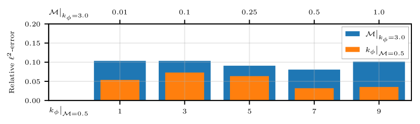
(a) Linear convection-diffusion case.

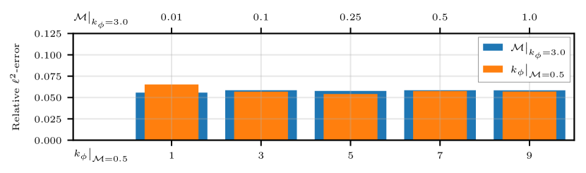
(b) Nonlinear convection-diffusion case.

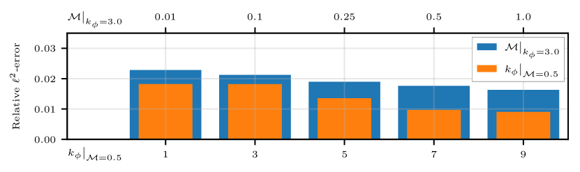
(c) Two-dimensional turbulent flow case.

Figure 4: Robustness analysis. Results for the parameterised studies for each of the three partial differential equations. Orange-bars denote results for case $\mathit{(i)}$: fixing the magnitude and varying the Rastrigin wavenumber. Blue-bars denote results for case $\mathit{(ii)}$: fixing the Rastrigin wavenumber and varying the magnitude.

6 Physical consistency of uncovered Navier-Stokes solutions

Results in section §5.4 show that, for a generic training setup, we are able to achieve low values of the relative error regardless of modality or magnitude of systematic error. Because the two-dimensional turbulent flow case is chaotic, infinitesimal errors $\mathcal{O}({\epsilon})$ exponentially grow in time, therefore, the residual $\mathcal{R}({\bm{u}}^{\ast}(\bm{\Omega}_{g},t)+{\epsilon}(\bm{\Omega}_{g},t);\lambda)\gg\mathcal{R}({\bm{u}}^{\ast}(\bm{\Omega}_{g},t);\lambda)$ where ${\epsilon}$ is a perturbation parameter. In this section, we analyse the physical properties of the solutions of the Navier-Stokes equation (Eq. 18) uncovered by the PC-CNN, ${\bm{\eta_{\theta}}}({\bm{\zeta}}(\bm{\Omega}_{g},t)))$.

First, we show snapshots of the time evolution of the two-dimensional turbulent flow in Figure 5. These confirms that the model is learning a physical solution across the time-domain of the solution, as shown in the error on a log-scale in the final column. The parameterisation of the systematic error is fixed in this case with $k_{\phi}=7,\mathcal{M}=0.5$.

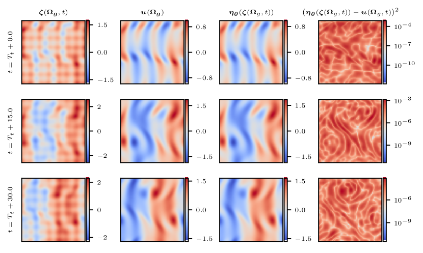
Figure 5: Systematic error removal for the two-dimensional turbulent flow $[k_{\phi}=7,\mathcal{M}=0.5]$. $T_{t}$ denotes the length of the transient.

Second, we analyse the statistics of the solution. The mean kinetic energy of the flow at each timestep is directly affected by the introduction of the systematic error. In the case of our strictly positive systematic error ${\bm{\phi}}(\bm{\Omega}_{g})$, the mean kinetic energy is increased at every point. Results in Figure 6 show the kinetic energy time series across the time-domain for (i) the ground truth ${\bm{u}}^{\ast}(\bm{\Omega}_{g},t)$; the corrupted data ${\bm{\zeta}}(\bm{\Omega}_{g},t)$; and the network’s predictions ${\bm{\eta_{\theta}}}({\bm{\zeta}}(\bm{\Omega}_{g},t))$. The chaotic nature of the solution can be observed from the spikes in chaotic energy. We observe that the network predictions accurately reconstruct the kinetic energy trace across the simulation domain, despite fewer than $2\%$ of the available timesteps being used for training.

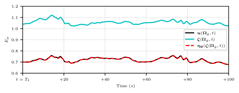
Figure 6: Kinetic energy for the two-dimensional turbulent flow $[k_{\phi}=7,\mathcal{M}=0.5]$.

Third, we analyse the energy spectrum, which is characteristic of turbulent flows, in which the energy content decreases with the wavenumber. Introducing the systematic error at a particular wavenumber artificially alters the energy spectrum due to increased energy content. In Figure 7, we show the energy spectrum for the two-dimensional turbulent flow, where this unphysical spike in energy content is visible for $\lvert\bm{k}\rvert\geq 7$. Model predictions ${\bm{\eta_{\theta}}}({\bm{\zeta}}(\bm{\Omega}_{g},t))$ correct the energy content for $\lvert\bm{k}\rvert<21$, and successfully characterise and reproduce scales of turbulence. The exponential decay of energy content with increasing spatial frequency provides a significant challenge for the residual-based loss. Despite the challenge, we observe only minor discrepancy from the true solution at large wavenumbers, i.e., when aliasing occurs ($\lvert\bm{k}\rvert\gtrapprox 29$).

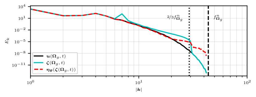
Figure 7: Energy Spectrum for the two-dimensional turbulent flow $[k_{\phi}=7,\mathcal{M}=0.5]$.

The ability of the network ${\bm{\eta_{\theta}}}$ to recover the underlying solution from corrupted data is demonstrated to yield low-error when compared with the true underlying solution of the partial differential equation. By investigating properties and statistics of the solution we demonstrate that, even for turbulent nonlinear systems, we are able to produce predictions that adhere to the physical properties of the system.

7 Conclusion

Data and models can be corrupted by systematic errors, which may originate from miscalibration of the experimental apparatus and epistemic uncertainties. We introduce a methodology to remove the systematic error from data to uncover the physical solution of the partial differential equation. First, we introduce the physics-constrained convolutional neural network (PC-CNN), which provides the means to compute the physical residual, i.e., the areas of the field in which the physical laws are violated because of the systematic error. Second, we formulate an optimisation problem by leveraging prior knowledge of the underlying physical system to regularise the predictions from the PC-CNN. Third, we numerically test the method to remove systematic errors from data produced by three partial differential equations of increasing complexity (linear and nonlinear diffusion-convection, and Navier-Stokes). This shows the ability of the PC-CNN to accurately recover the underlying solutions. Fourth, we carry out a parameterised analysis, which successfully minimises the relative error for a variety of systematic errors with different magnitudes and degrees of multimodality. This shows that the method is robust. Finally, we investigate the physical consistency of the inferred solutions for the two-dimensional turbulent flow. The network predictions satisfy physical properties of the underlying partial differential equation (Navier-Stokes), such as the statistics and energy spectrum. This work opens opportunities for inferring solutions of partial differential equations from sparse measurements. Current work is focused on scaling up the framework to three-dimensional flows, and dealing with experimental data.

References

- Sciacchitano et al. [2015] A. Sciacchitano, D. R. Neal, B. L. Smith, S. O. Warner, P. P. Vlachos, B. Wieneke, and F. Scarano, “Collaborative framework for piv uncertainty quantification: comparative assessment of methods,” Measurement Science and Technology, vol. 26, no. 7, p. 074004, 2015.
- Zucchelli et al. [2021] E. M. Zucchelli, E. D. Delande, B. A. Jones, and M. K. Jah, “Multi-fidelity orbit determination with systematic errors,” The Journal of the Astronautical Sciences, vol. 68, pp. 695–727, 2021.
- Adrian [1991] R. J. Adrian, “Particle-imaging techniques for experimental fluid mechanics,” Annual review of fluid mechanics, vol. 23, no. 1, pp. 261–304, 1991.
- Vedula and Adrian [2005] P. Vedula and R. J. Adrian, “Optimal solenoidal interpolation of turbulent vector fields: Application to ptv and super-resolution piv,” Experiments in Fluids, vol. 39, pp. 213–221, 8 2005.
- Schiavazzi et al. [2014] D. Schiavazzi, F. Coletti, G. Iaccarino, and J. K. Eaton, “A matching pursuit approach to solenoidal filtering of three-dimensional velocity measurements,” Journal of Computational Physics, vol. 263, pp. 206–221, 4 2014.
- Kochkov et al. [2021] D. Kochkov, J. A. Smith, A. Alieva, Q. Wang, M. P. Brenner, and S. Hoyer, “Machine learning–accelerated computational fluid dynamics,” Proceedings of the National Academy of Sciences, vol. 118, no. 21, p. e2101784118, 2021.
- Kumar and Nachamai [2017] N. Kumar and M. Nachamai, “Noise removal and filtering techniques used in medical images,” Oriental journal of computer science and technology, vol. 10, pp. 103–113, 3 2017.
- Raiola et al. [2015] M. Raiola, S. Discetti, and A. Ianiro, “On piv random error minimization with optimal pod-based low-order reconstruction,” Experiments in Fluids, vol. 56, 4 2015.
- Mendez et al. [2017] M. A. Mendez, M. Raiola, A. Masullo, S. Discetti, A. Ianiro, R. Theunissen, and J. M. Buchlin, “Pod-based background removal for particle image velocimetry,” Experimental Thermal and Fluid Science, vol. 80, pp. 181–192, 1 2017.
- Vincent et al. [2008] P. Vincent, H. Larochelle, Y. Bengio, and P.-A. Manzagol, “Extracting and composing robust features with denoising autoencoders,” Proceedings of the 25th International Conference on Machine Learning, pp. 1096–1103, 2008.
- Freeman et al. [2002] W. T. Freeman, T. R. Jones, and E. C. Pasztor, “Example-based super-resolution,” IEEE Computer Graphics and Applications, vol. 22, pp. 56–65, 2002.
- Yang et al. [2010] J. Yang, J. Wright, T. S. Huang, and Y. Ma, “Image super-resolution via sparse representation,” IEEE Transactions on Image Processing, vol. 19, pp. 2861–2873, 11 2010.
- Dong et al. [2014] C. Dong, C. C. Loy, K. He, and X. Tang, “Learning a deep convolutional network for image super-resolution,” Computer Vision – ECCV 2014184, pp. 184–199, 2014. [Online]. Available: http://mmlab.ie.cuhk.edu.hk/projects/SRCNN.html.
- Xie et al. [2018] Y. Xie, E. Franz, M. Chu, and N. Thuerey, “Tempogan: A temporally coherent, volumetric gan for super-resolution fluid flow,” ACM Transactions on Graphics, vol. 37, 2018.
- Hornik et al. [1989] K. Hornik, M. Stinchcombe, and H. White, “Multilayer feedforward networks are universal approximators,” Neural Networks, vol. 2, pp. 359–366, 1989.
- Zhou [2020] D. X. Zhou, “Universality of deep convolutional neural networks,” Applied and Computational Harmonic Analysis, vol. 48, pp. 787–794, 3 2020.
- Lagaris et al. [1998] I. E. Lagaris, A. Likas, and D. I. Fotiadis, “Artificial neural networks for solving ordinary and partial differential equations,” IEEE Transactions on Neural Networks, vol. 9, pp. 987–1000, 1998.
- Raissi et al. [2019] M. Raissi, P. Perdikaris, and G. E. Karniadakis, “Physics-informed neural networks: A deep learning framework for solving forward and inverse problems involving nonlinear partial differential equations,” Journal of Computational Physics, vol. 378, pp. 686–707, 2 2019.
- Rastrigin [1974] L. A. Rastrigin, “Systems of extremal control,” Nauka, 1974.
- Nóvoa and Magri [2022] A. Nóvoa and L. Magri, “Real-time thermoacoustic data assimilation,” Journal of Fluid Mechanics, vol. 948, p. A35, 2022.
- LeCun et al. [2015] Y. LeCun, Y. Bengio, and G. Hinton, “Deep learning,” nature, vol. 521, no. 7553, pp. 436–444, 2015.
- Gu et al. [2018] J. Gu, Z. Wang, J. Kuen, L. Ma, A. Shahroudy, B. Shuai, T. Liu, X. Wang, G. Wang, J. Cai, and T. Chen, “Recent advances in convolutional neural networks,” Pattern Recognition, vol. 77, pp. 354–377, 2018. [Online]. Available: https://www.sciencedirect.com/science/article/pii/S0031320317304120
- Pope and Pope [2000] S. B. Pope and Pope, Turbulent flows. Cambridge university press, 2000.
- Racca et al. [2022] A. Racca, N. A. K. Doan, and L. Magri, “Modelling spatiotemporal turbulent dynamics with the convolutional autoencoder echo state network,” 2022.
- Doan et al. [2021] N. A. K. Doan, W. Polifke, and L. Magri, “Short and long-term predictions of chaotic flows and extreme events: a physics-constrained reservoir computing approach,” Proceedings of the Royal Society A: Mathematical, Physical and Engineering Sciences, vol. 477, no. 2253, p. 20210135, 2021.
- Magri [2023] L. Magri, “Introduction to neural networks for engineering and computational science,” 1 2023.
- Murata et al. [2020] T. Murata, K. Fukami, and K. Fukagata, “Nonlinear mode decomposition with convolutional neural networks for fluid dynamics,” Journal of Fluid Mechanics, vol. 882, p. A13, 2020.
- Gao et al. [2021] H. Gao, L. Sun, and J.-X. Wang, “Super-resolution and denoising of fluid flow using physics-informed convolutional neural networks without high-resolution labels,” Physics of Fluids, vol. 33, p. 073603, 7 2021.
- Bishop [1994] C. M. Bishop, “Neural networks and their applications,” Review of Scientific Instruments, vol. 65, no. 6, pp. 1803–1832, 1994.
- Aloysius and Geetha [2017] N. Aloysius and M. Geetha, “A review on deep convolutional neural networks,” pp. 0588–0592, 2017.
- Kelshaw [2022] D. Kelshaw, “Kolsol,” https://github.com/magrilab/kolsol, 2022.
- Canuto et al. [1988] C. Canuto, M. Y. Hussaini, A. Quarteroni, and T. A. Zang, Spectral Methods in Fluid Dynamics. Springer Berlin Heidelberg, 1988.
- Bateman [1915] H. Bateman, “Some recent researches on the motion of fluids,” Monthly Weather Review, vol. 43, no. 4, pp. 163 – 170, 1915.
- Burgers [1948] J. Burgers, “A mathematical model illustrating the theory of turbulence,” vol. 1, pp. 171–199, 1948.
- Fylladitakis [2018] E. D. Fylladitakis, “Kolmogorov flow: Seven decades of history,” Journal of Applied Mathematics and Physics, vol. 6, pp. 2227–2263, 2018.
- Kingma and Ba [2015] D. P. Kingma and J. Ba, “Adam: A method for stochastic optimization,” 2015.
- Majda and Kramer [1999] A. J. Majda and P. R. Kramer, “Simplified models for turbulent diffusion: theory, numerical modelling, and physical phenomena,” Physics reports, vol. 314, no. 4-5, pp. 237–574, 1999.