Multifractality in spin glasses

Abstract

We unveil the multifractal behavior of Ising spin glasses in their low-temperature phase. Using the Janus II custom-built supercomputer, the spin-glass correlation function is studied locally. Dramatic fluctuations are found when pairs of sites at the same distance are compared. The scaling of these fluctuations, as the spin-glass coherence length grows with time, is characterized through the computation of the singularity spectrum and its corresponding Legendre transform. A comparatively small number of site pairs controls the average correlation that governs the response to a magnetic field. We explain how this scenario of dramatic fluctuations (at length scales smaller than the coherence length) can be reconciled with the smooth, self-averaging behavior that has long been considered to describe spin-glass dynamics.

The notion of multifractality Frisch and Parisi (1985); Harte (2001) refers to situations where many different fractal behaviors coexist within the same system. A major role is played in this context by scale symmetry, see, e.g., Wilson (1979); Parisi (1988); Barnsley (2012): in many situations in physics, chemistry and beyond, apparently random objects look the same when the observation scale is changed. The scale change is often quantitatively characterized through a number, the fractal dimension. Multifractals (as opposed to fractals) are systems that need many fractal dimensions to get their scaling properties fully characterized.

Some of the first examples of multifractal behavior appeared in physics, in the contexts of turbulence Benzi et al. (1984), Anderson localization Castellani and Peliti (1986) and diffusion-limited aggregates Stanley and Meakin (1988). A unifying language was soon introduced in a study of chaotic dynamics Halsey et al. (1986a, b). The concept has gained popularity as the list of systems exhibiting some form of multifractality has steadily grown. To name only a few, let us recall surface growth Barabási and Stanley (2009), human heartbeat dynamics Ivanov et al. (1999), mating copepods Seuront and Stanley (2014); Klopper (2014), rainfall Deidda (2000) or the analysis of financial time series Alvarez-Ramirez et al. (2008).

Here we add a (perhaps) surprising member to the list: the off-equilibrium dynamics of spin-glass systems Mydosh (1993); Charbonneau et al. (2023). These disordered magnetic alloys have long been regarded as a paradigmatic toy model for the study of glassiness, optimization, biology, financial markets or social dynamics. It is surprising that such a prominent feature as multifractality has gone unnoticed for such a well-studied model.

The explanation for the above paradox rests on the finite coherence length $\xi({t_{\mathrm{w}}})$ that develops when a spin glass, initially at some very high temperature, is suddenly cooled below the critical temperature $T_{\mathrm{c}}$, and let to relax for a waiting time ${t_{\mathrm{w}}}$—most experimental work on spin glasses is carried out under non-equilibrium conditions Vincent et al. (1997). As ${t_{\mathrm{w}}}$ increases, glassy domains of growing size $\xi({t_{\mathrm{w}}})$ develop, see Fig. 1. The growth of $\xi({t_{\mathrm{w}}})$ is sluggish for a spin glass, reaching only $\xi\sim$ 200 lattice spacings for ${t_{\mathrm{w}}}\sim$1 hour Zhai et al. (2019, 2020). Now, when one measures the magnetic response to an external field, which is the main experimental probe of spin-glass dynamics, an average over the whole sample is carried out. Since the sample is effectively composed of many independent domains of linear size $\sim\xi({t_{\mathrm{w}}})$, the central limit theorem eliminates from the average response the large fluctuations that could ultimately cause multifractal behavior. With few exceptions (see below), most numerical work has emphasized the space-averaged correlation function in Fig. 1. Besides, see Methods, studying correlations without spatial averages is very demanding computationally.

It follows from the above considerations that multifractal behavior in spin glasses should be investigated in large statistical deviations that occur at a length scale smaller than (or comparable to) $\xi({t_{\mathrm{w}}})$, definitively not the standard framework either for experiments(see Zhai et al., 2020; Paga et al., 2021; Zhai et al., 2022, for instance) or for simulations Belletti et al. (2008a); Baity-Jesi et al. (2017, 2018). There is, however, an important exception. Recently, progress has been achieved Baity-Jesi et al. (2023) in the theoretical interpretation of the experimental rejuvenation and memory effects in spin glasses Jonason et al. (1998). Crucial for this achievement was the study of temperature chaos in the off-equilibrium dynamics at the $\xi({t_{\mathrm{w}}})$ length scale Baity-Jesi et al. (2021), through numerical simulations using the Janus II dedicated supercomputer Baity-Jesi et al. (2014a). As we shall show below, the consideration of fluctuations at the $\xi({t_{\mathrm{w}}})$ length scale still holds surprises.

Specifically, we shall consider the spin-glass correlation function, see Methods for definitions. The space-averaged correlation function is a well-known quantity and the basis for the computation of $\xi({t_{\mathrm{w}}})$ explained in Fig. 1. We shall depart from the standard approach, however, by avoiding the spatial average. We shall compute the correlation function for a pair of sites ${{\bm{x}}}$ and ${{\bm{y}}}$, and consider the statistical fluctuations induced by varying ${{\bm{x}}}$ while fixing ${\bm{r}}={\bm{y}}-{\bm{x}}$.

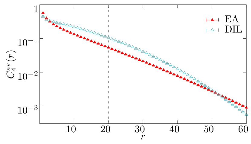
Figure 1: The correlation function, (10), as computed for the three-dimensional Ising diluted ferromagnet (DIL) and for the Ising spin glass (EA), versus distance $r$. Data were obtained in systems of linear size $L=160$ with coherence length $\xi({t_{\mathrm{w}}})=20$ (dashed vertical line) at temperature $T=0.9$—recall that $T_{\mathrm{c}}\approx 1.1$ for EA Baity-Jesi et al. (2013). As explained in Methods, the coherence length is computed from the integral $I_{2}=\int_{0}^{\infty}r^{2}C^{\text{av}}_{4}(r)\mathrm{d}r$ (the integrand is shown in the Supporting Information).

The reader may argue that it is difficult to find large statistical fluctuations in a mathematical object bounded between 0 and 1, such as the spin-glass correlation function. A moment of thought will reveal that large fluctuations are only possible if the average of the correlation function goes to zero as $\xi({t_{\mathrm{w}}})$ grows, so that the correlation function at a given site can get large if measured in units of the averaged correlation.

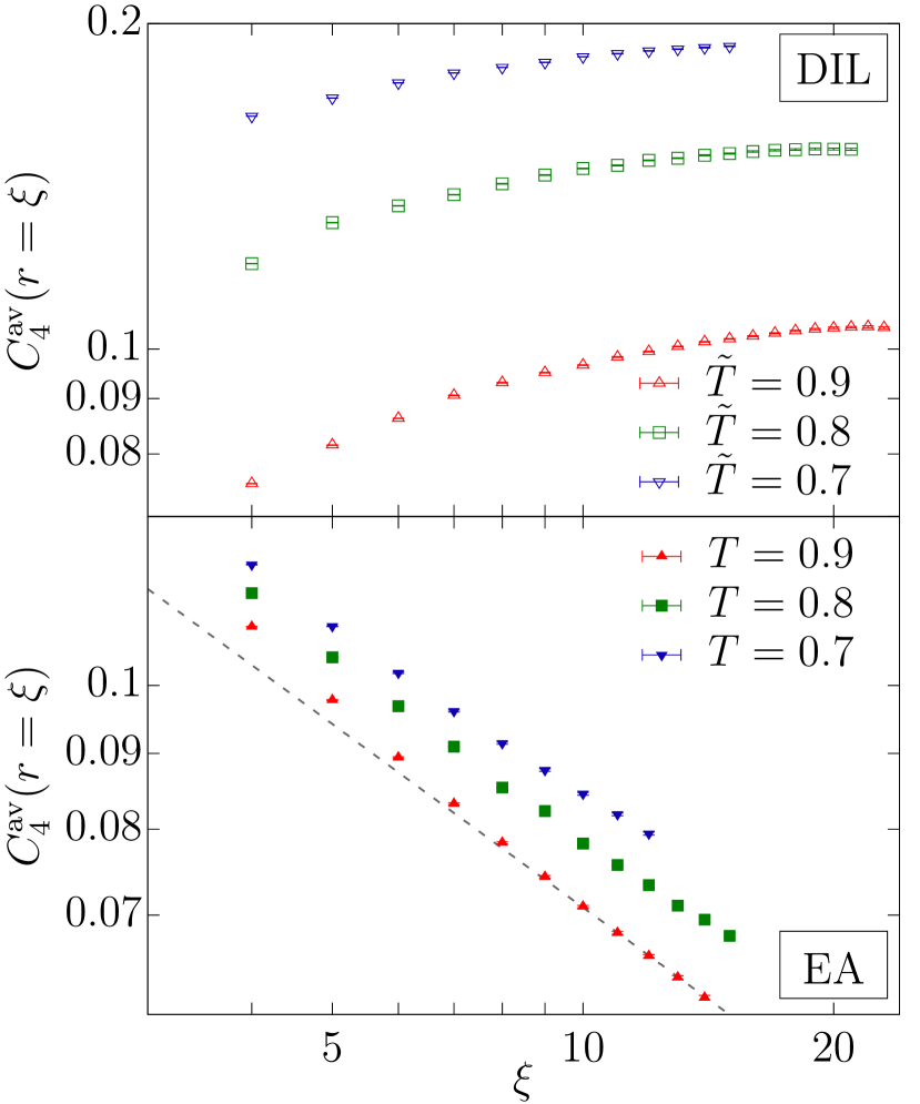
Figure 2: Correlation function $C_{4}^{\text{av}}(r=\xi({t_{\mathrm{w}}}))$, see  (10) versus the coherence length $\xi({t_{\mathrm{w}}})$, as computed for DIL (top) and for EA (bottom) at temperatures $T,\ \tilde{T}=0.9,0.8$ and $0.7$ (see Methods for a complete definition of $\tilde{T}$). Error bars are smaller than the point size. The dashed line is our fit to (2), with $q=1$, for EA at $T=0.9$ (to avoid scaling corrections, we fit in the range $\xi({t_{\mathrm{w}}})\in[10,20]$, see SI for further information). Note that, while the DIL $C_{4}^{\text{av}}(r=\xi({t_{\mathrm{w}}}))$ tends to a $T$-dependent positive limit for large coherence length (which excludes multiscaling at $T<T_{\text{c}}$), the spin-glass correlation functions steadily decrease with $\xi({t_{\mathrm{w}}})$.

Indeed, spin glasses are peculiar among systems with domain-growth off-equilibrium dynamics. Fig. 2 compares the space-averaged correlation function at distance $r=\xi({t_{\mathrm{w}}})$ for two Ising systems in space dimension $D=3$, the link-diluted ferromagnet and the spin glass. In the ferromagnet, the correlation function goes to a constant value (the squared spontaneous magnetization) as $\xi$ grows. Hence, large deviations and multifractality are possible for the ferromagnet only at $T_{\mathrm{c}}$, where the spontaneous magnetization vanishes . In the spin glass, instead, the correlation function scales as $1/r^{\theta}$ for distances up to $r\sim\xi$ . Hence, unlike the diluted ferromagnet, the spin glass can accommodate large fluctuations for all $T<T_{\mathrm{c}}$. This is why here we decide to focus on the spin glass.

Results

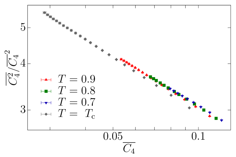
Figure 3: Ratio of the second moment of the spin-glass correlation function $C_{4}$ computed at $r=\xi({t_{\mathrm{w}}})$, $\overline{C_{4}^{2}}$, to the squared first moment, $\overline{C_{4}}^{2}$, as a function of $\overline{C_{4}}$. We show the data for all temperatures considered in this work. $\overline{C_{4}}$ tends to zero as the coherence length $\xi({t_{\mathrm{w}}})$ gets large, recall Fig. 2. Note that $\overline{C_{4}^{2}}/\overline{C_{4}}^{2}$ scales with $\overline{C_{4}}$ as a power law, which indicates that in the scaling limit (i.e., $\xi({t_{\mathrm{w}}})\to\infty$ or $\overline{C_{4}}\to 0$) the order of magnitude of $\overline{C_{4}^{2}}$ is larger than the one of $\overline{C_{4}}^{2}$. Data in the glassy phase, $T<T_{\mathrm{c}}$, roughly follow the same scaling curve. At the critical point there is still a power type relation with a slightly different exponent. Error bars are smaller than the points size. The same data are shown as a function of $\xi({t_{\mathrm{w}}})$ in the SI.

The first indication of large deviations in the statistics of the spin-glass correlation function $C_{4}$ is shown in Fig. 3, where we select the distance $r=\xi({t_{\mathrm{w}}})$. The ratio of the second moment of $C_{4}$, $\overline{C_{4}^{2}}$, to the first moment squared, $\overline{C_{4}}^{2}$, nicely follows a power law as a function of $\overline{C_{4}}$ (this type of analysis was pioneered in Benzi et al., 1993). If continued to $\overline{C_{4}}\to 0$ (i.e., as $\xi({t_{\mathrm{w}}})$ grows, see Fig. 2), this power law implies that the orders of magnitude of $\overline{C_{4}^{2}}$ and $\overline{C_{4}}^{2}$ differ in the large-$\xi({t_{\mathrm{w}}})$ scaling limit. This behavior is not reminiscent of a monofractal, which in the scaling limit is characterized by a single quantity (say, $\overline{C_{4}}$).

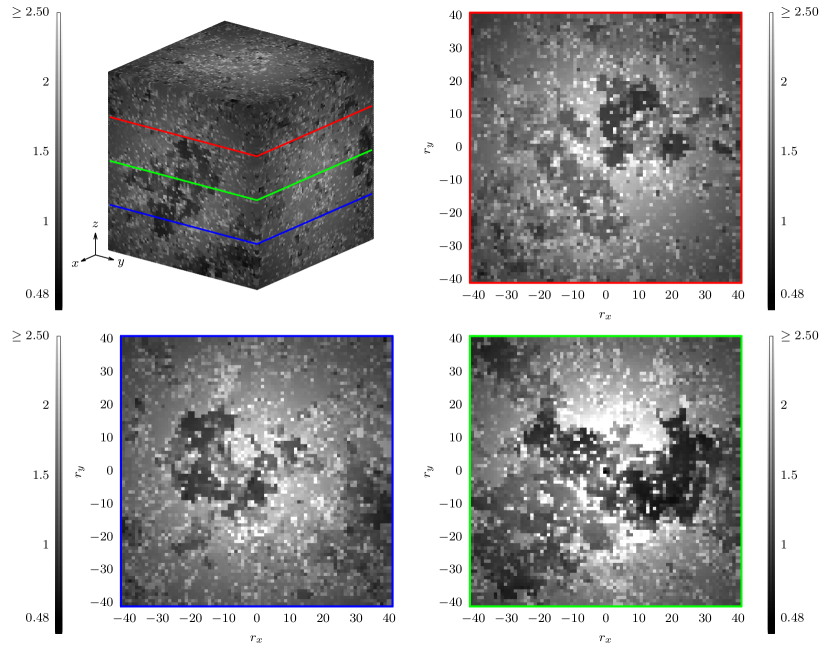
Figure 4: Grayscale representation of the order-of-magnitude modulating factor $M({\bm{x}},{\bm{r}},{t_{\mathrm{w}}})$, see (1), computed for site ${\bm{x}}=(64,64,64)$ of a sample with coherence length $\xi({t_{\mathrm{w}}})=20$, at $T=0.9$, with an ${N_{\mathrm{R}}}=512$ estimator (see Methods). We show results for displacement vectors ${\bm{r}}=(r_{x},r_{y},r_{z})$ in a cube $-40\leq r_{x},r_{y},r_{z}\leq 40$. The top-left panel depicts the three visible faces of the cube, while the other three panels show sections at $r_{z}=-20,0,20$, respectively. Our color code is darker the smaller $M({\bm{x}},{\bm{r}},{t_{\mathrm{w}}})$ (hence, the more slowly correlations decay with distance). For ease of representation, we have chosen a color code linear between the minimal value of $M({\bm{x}},{\bm{r}},{t_{\mathrm{w}}})$ and 2.5. Displacements ${\bm{r}}$ with $M({\bm{x}},{\bm{r}},{t_{\mathrm{w}}})>2.5$ are depicted as if $M({\bm{x}},{\bm{r}},{t_{\mathrm{w}}})=2.5$. See SI for more examples of this modulating factor.

We also note from Fig. 3 that all our data with $T<T_{\mathrm{c}}$ follow the same scaling curve, which slightly differs from its counterpart at the critical point. This is not completely unexpected, because the $\epsilon$-expansion tells us that the average $C_{4}$ at $T_{\text{c}}$ decays as a power law with distance with an exponent Chen and Lubensky (1977) that is twice as large as the exponent for $T<T_{\text{c}}$ De Dominicis and Kondor (1989). In fact, we lack an explanation for the similarity of the two exponents that can be observed in Fig. 3. From now on, our analysis will focus on our data at $T=0.9$, namely the temperature in the spin-glass phase where we are able to reach the largest $\xi({t_{\mathrm{w}}})$.

A picture of the physical situation is presented in Fig. 4. We may expect a different behavior for the average and the local correlation function when distances up to $r\sim\xi({t_{\mathrm{w}}})$ are considered ($\theta(T=0.9)\approx 0.4$ Baity-Jesi et al. (2018)) :

$$C_{4}^{\text{av}}(r,{t_{\mathrm{w}}})\sim\frac{1}{r^{\theta}}\,,\quad C_{4}({\bm{x}},{\bm{x}}+{\bm{r}};{t_{\mathrm{w}}})\sim\frac{1}{r^{\theta M({\bm{x}},{\bm{r}},{t_{\mathrm{w}}})}}\,.$$ (1)

As the reader can check from Fig. 4, the order-of-magnitude modulating factor $M({\bm{x}},{\bm{r}},{t_{\mathrm{w}}})$ varies by a factor of 16, which indicates that there are site pairs $({\bm{x}},{\bm{x}}+{\bm{r}})$ a lot more —or a lot less— correlated than the average. In fact, see Fig. 5, the median correlation function at distance $r=\xi({t_{\mathrm{w}}})$, scales as $[C_{4}^{\text{av}}]^{a}$, with $a\approx 1.5$. In other words, the typical correlation function is a lot smaller than the average value.

In order to make the above qualitative description quantitative, we consider the moments of the probability distribution of $C_{4}$ at distance $r=\xi({t_{\mathrm{w}}})$. The $q$-th moment turns out to follow a scaling law

$$\overline{C_{4}^{q}}\sim\frac{A_{q}}{\xi^{\tau(q)}}\,.$$ (2)

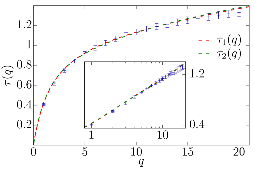
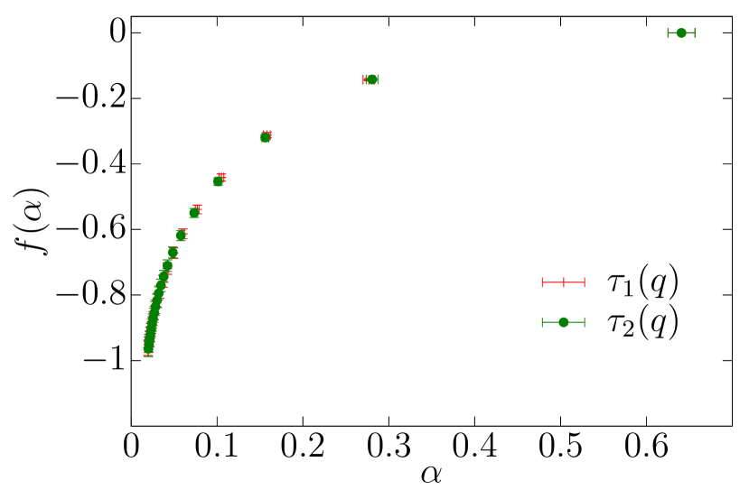
Figure 6: Scaling exponent $\tau(q)$ for the $q$-th moment $\overline{C_{4}(r=\xi)^{q}}\sim\xi^{-\tau(q)}$ computed from simulations of the Ising spin glass at $T=0.9$ (see SI for results at $T_{\mathrm{c}}$). The non-linear behavior is a strong indication of multifractality. The dashed lines are fits to the functional forms in (3) (the goodness-of-fit statistics are presented in the SI). The inset presents the same data as a function of $\log(q)$.

Figure 7: Legendre transformation $f(\alpha)$ of function $\tau(q)$, see (7), as a function $\alpha=\mathrm{d}\tau/\mathrm{d}q$, computed from the fitting ansätze in (3). Errors on both axes have been obtained as explained in Methods (for further details, see Yllanes, 2011). Since $f(\alpha)$ is the large-deviations function of the decay rate $C_{4}(r=\xi)\sim r^{-\alpha}$, the data show that the majority of sites have the median decay rate of approximately $0.65$, much larger than the mean decay rate $\alpha\approx 0.4$.

Fig. 7 shows the $\tau(q)$ function, which significantly differs from the monofractal behavior $\tau^{\text{mono}}(q)=q\,\tau^{\text{mono}}(1)$. It is this departure from linear behavior that justifies using the term multifractal to describe spin-glass dynamics (see, e.g., Halsey et al., 1986a).

For large moments, $\tau(q)$ seems to grow as $\log q$ (see the inset in Fig. 7). The origin of this logarithmic growth seems to be in the behavior of the probability distribution function $P(C_{4})$ near $C_{4}=1$. As shown in the Supporting Information (SI), the numerical data are consistent with $P(C_{4})\propto(1-C_{4})^{B(\xi)}$ for $C_{4}$ close to 1, with an exponent that grows as $B(\xi({t_{\mathrm{w}}}))\sim\log\xi({t_{\mathrm{w}}})$. This behavior of the correlation function would explain the observed logarithmic growth of $\tau(q)$. However, just to be on the safe side, we have tried two different functional forms to fit the numerical data in Fig. 7:

$$\tau_{1}(q)=mq\frac{1+c_{1}q}{1+c_{2}q}\,,\quad\tau_{2}(q)=mq\frac{1+d_{1}q\log q}{(1+d_{2}q)^{2}}\,.$$ (3)

Both $\tau_{1}$ and $\tau_{2}$ have the same derivative $m$ at $q\!=\!0$. We do not treat $m$ as a fitting parameter. Rather we take it from the scaling of the median of the distribution $P(C_{4})$ with $\xi$ (see SI). Although both $\tau_{1}(q)$ and $\tau_{2}(q)$ make an excellent job at fitting our data (see again SI), only $\tau_{2}(q)$ displays the logarithmic growth with $q$, at large $q$, that we find more plausible.

Discussion

Following Ref. Halsey et al. (1986a), we shall discuss our results in terms of a different stochastic variable, $\alpha=\log C_{4}(r=\xi({t_{\mathrm{w}}}))/\log[1/\xi({t_{\mathrm{w}}})]$, so that (we drop the argument in $\xi$ for the sake of shortness)

$$C_{4}=\frac{1}{\xi^{\alpha}}\,,\quad P(C_{4})\frac{\mathrm{d}C_{4}}{\mathrm{d}\alpha}\sim\xi^{f(\alpha)}\,.$$ (4)

(4) defines the large-deviations function $f(\alpha)$. Then, we find for the moments of $C_{4}$

$$\overline{C_{4}^{q}}=\int_{0}^{1}\text{d}C_{4}\,P(C_{4})C_{4}^{q}\sim\int_{0}^{\infty}\text{d}\alpha\,\text{e}^{\log(\xi)[f(\alpha)-q\alpha]}\,.$$ (5)

For large $\xi$, the above integral is dominated by the maximum of $[f(\alpha)-q\alpha]$ at some value $\alpha=\alpha^{*}$:

$$\overline{C_{4}^{q}}\sim\frac{1}{\xi^{-[f(\alpha^{*})-q\alpha^{*}]}}\,.$$ (6)

Comparing with (2), we realize that $f(\alpha)$ is just (minus) the Legendre transform of the singularity spectrum $\tau(q)$:

$$f(\alpha)=-\max_{q}\big{[}\tau(q)\,-\,q\alpha\big{]}.$$ (7)

We show $f(\alpha)$ in Fig. 7, as computed from our fitting ansätze $\tau_{1}(q)$ and $\tau_{2}(q)$, in (3). In the range of Fig. 7 —since $\alpha(q)=\tau^{\prime}(q)$— the results from the two ansätze can hardly be distinguished. The two, however, differ in that the range of $\alpha$ for $\tau_{2}(q)$ goes all the way down to $\alpha=0$ (because $\alpha_{2}(q)=\mathrm{d}\tau_{2}/\mathrm{d}q\sim 1/q$). Indeed, if $\tau(q)$ goes as $\log(q)$ for large $q$, then the large-deviations function goes as $f(\alpha\to 0)\sim\log(\alpha)$.

Let us recapitulate: the probability of finding a site ${\bm{x}}$ with $C_{4}({\bm{x}},{\bm{x}}+{\bm{r}})$ scaling as $1/r^{\alpha}$ for $r\sim\xi$ goes in the scaling limit as $\xi^{f(\alpha)}$. There are, hence, a lot more sites displaying the median scaling exponent $\alpha\approx 0.65$ than there are for the average scaling $\alpha\approx 0.4$ (because $f(0.65)>f(0.4)$, recall Fig. 5). The larger $\xi({t_{\mathrm{w}}})$ grows, the more pronounced this difference is. Thus, the expression “silent majority” Baity-Jesi et al. (2014b) could be aptly employed to describe spin-glass dynamics: the central limit theorem ensures that it is the (somewhat exceptional) average value the one that can be measured on length scales larger than $\xi({t_{\mathrm{w}}})$ (hence, in experiments). The experimental-scale dynamics is, however, not completely blind to these short-scale fluctuations. Indeed, temperature chaos Baity-Jesi et al. (2021) —and, hence, rejuvenation Baity-Jesi et al. (2023), which is certainly experimentally observable (see, e.g., Jonason et al., 1998)— is ruled by statistical fluctuations at the scale of $r$ smaller than, or similar to, $\xi({t_{\mathrm{w}}})$.

Our data show that varying $T$ simply changes $\tau(q)$ by an essentially constant factor [e.g., $\tau(q,T_{\mathrm{c}})\approx 1.5\tau(q,T=0.9)$, see SI]. Furthermore, Fig. 3 makes us confident that, taking $\overline{C_{4}}$ as scaling variable instead of $\xi({t_{\mathrm{w}}})$, the overall picture is essentially temperature independent for $T<T_{\mathrm{c}}$.

Whether or not multifractal behavior is also present in equilibrium correlation functions in the spin-glass phase stands out as an interesting open question. Statics-dynamics equivalence Franz et al. (1998); Alvarez Baños et al. (2010); Wittmann and Young (2016); Baity-Jesi et al. (2017) suggests that the answer will be positive.

As a final remark, let us stress that ongoing efforts to build a mathematically rigorous theory of non-equilibrium spin-glass dynamics through the concept of the maturation metastate (see Jensen et al., 2021 and references therein) should take into account the extreme spatial heterogeneity unveiled in this work.

Methods

Model and simulations

We focus on the Edwards-Anderson model (EA) in a simple cubic lattice with linear size $L=160$ and periodic boundary conditions. Our $S_{{\bm{x}}}=\pm 1$ spin, placed at the lattice sites, interact with their nearest neighbors through the Hamiltonian:

$$\mathcal{H}=-\sum_{\langle{\bm{x}},{\bm{y}}\rangle}J_{{\bm{x}},{\bm{y}}}S_{{\bm{x}}}S_{{\bm{y}}}\,.$$ (8)

The coupling constants $J_{{\bm{x}},{\bm{y}}}$ are independent random variables ($J_{{\bm{x}},{\bm{y}}}=\pm 1$ with equal probability), fixed once and for all at the beginning of the simulation (this is named quenched disorder). A realization of the couplings is called a sample. We shall use 16 samples in this work. In general, errors will be computed with a jackknife method over the samples (see, for instance, Amit and Martín-Mayor, 2005; Yllanes, 2011). We have also considered a diluted Ising model (see below), as a baseline model displaying domain-growth off-equilibrium dynamics.

We have simulated the model in (8) through a Metropolis dynamics on the Janus II supercomputer Baity-Jesi et al. (2014a). Our time unit is a full-lattice sweep, roughly equivalent to a picosecond of physical time Mydosh (1993). The critical temperature for this model is $T_{\mathrm{c}}=1.1019(29)$ Baity-Jesi et al. (2013).

For each sample, we have simulated ${N_{\mathrm{R}}}=512$ statistically independent system copies or replicas. We denote by $\langle\cdots\rangle$ the average over thermal noise for one sample (as explained below, we obtain unbiased estimators of the thermal expectation values $\langle\cdots\rangle$ by averaging over the replicas). The subsequent average over samples is denoted by an overline ($\overline{\langle\cdots\rangle}$).

The main quantity of interest is the correlation function

$$C_{4}({\bm{x}},{\bm{y}},{t_{\mathrm{w}}})=\langle S_{{\bm{x}}}({t_{\mathrm{w}}})S_{{\bm{y}}}({t_{\mathrm{w}}})\rangle^{2}\,.$$ (9)

Note that, for a given sample and $({\bm{x}},{\bm{y}},{t_{\mathrm{w}}})$, $C_{4}({\bm{x}},{\bm{y}},{t_{\mathrm{w}}})$ is not a stochastic variable. However, it is a stochastic variable if we regard the variations induced by the choice of couplings $J_{{\bm{x}},{\bm{y}}}$ and over the considered sites $({\bm{x}},{\bm{y}},{t_{\mathrm{w}}})$. We term these stochastic variables $C_{4}$, without arguments.

As explained in the next paragraph, although $C_{4}({\bm{x}},{\bm{y}},{t_{\mathrm{w}}})$ cannot be computed with a finite number of replicas, unbiased estimators of its moments can be computed. In particular, previous work has mostly focused on the average correlation function

$$C_{4}^{\text{av}}({\bm{r}},{t_{\mathrm{w}}})=\frac{1}{L^{3}}\sum_{{\bm{x}}}\overline{C_{4}({\bm{x}},{\bm{y}}={\bm{x}}+{\bm{r}},{t_{\mathrm{w}}})}\,.$$ (10)

Cubic symmetry, present in averages over the samples, allows us to average over the three equivalent displacements ${\bm{r}}=(r,0,0)$ and permutations. We shall use the shorthand $C_{4}^{\text{av}}(r,{t_{\mathrm{w}}})$ to indicate this average over the three equivalent ${\bm{r}}$. To compute the coherence length $\xi({t_{\mathrm{w}}})$ we follow Belletti et al. (2008b, 2009); Baity-Jesi et al. (2018) and compute the integrals

$$I_{n}({t_{\mathrm{w}}})=\int_{0}^{\infty}r^{n}\,C^{\text{av}}_{4}(r,{t_{\mathrm{w}}})\mathrm{d}r\,.$$ (11)

Then, $\xi({t_{\mathrm{w}}})=I_{2}({t_{\mathrm{w}}})/I_{1}({t_{\mathrm{w}}})$.

As stated above, we have simulated, as a null experiment, the link-diluted Ising model (DIL). The only difference with the Hamiltonian in (8) is in the choice of the couplings: $J_{{\bm{x}},{\bm{y}}}=1$ (with $70\%$ probability) or $J_{{\bm{x}},{\bm{y}}}=0$ (with $30\%$ probability). Since all couplings are positive or zero, this is a ferromagnetic system without frustration. All our simulation and analysis procedures are identical for the DIL and EA models. The critical temperature is $T^{\text{DIL}}_{\mathrm{c}}=3.0609(5)$ Berche et al. (2004). Actually, this is twice the value reported in Berche et al. (2004) due to our use of an Ising, rather than Potts, formulation. In fact, with some abuse of language, in the main text we refer to DIL temperatures as $\tilde{T}=0.9$, $\tilde{T}=0.8$ or $0.7$ rather than to their real value $T^{\mathrm{DIL}}=\tilde{T}\,(T_{\mathrm{c}}^{\text{DIL}}/T_{\mathrm{c}}^{\text{EA}})$.

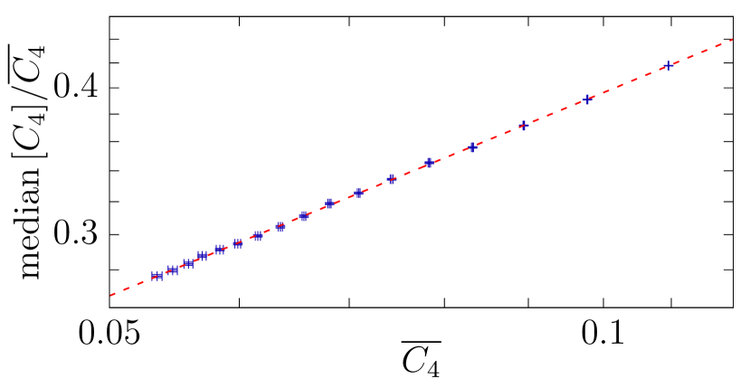
Figure 5: Median of the distribution $P[C_{4}(r=\xi)]$ in units of the first moment, $\overline{C_{4}}(r=\xi)$, versus $\overline{C_{4}}(r=\xi)$, as computed for the spin glass at temperature $T=0.9$. We show data in logarithmic scale. Therefore, the dashed line (a power-law fit with exponent $\sim 0.5$, see SI for details) appears as a straight line.

The range of coherence length and simulation times in this study can be found in Table 1.

Table 1: Maximum ${t_{\mathrm{w}}}$ and coherence length reached for each of our models and simulation temperatures.

$T$ or $\tilde{T}$	${t_{\mathrm{w}}}$(EA)	$\xi_{\mathrm{max}}$(EA)	${t_{\mathrm{w}}}$(DIL)	$\xi_{\mathrm{max}}$(DIL)
0.7	46531866276	12	498	15
0.8	18734780191	15	919	21
0.9	15172184825	20	954	23

Unbiased estimators of powers of $C_{4}({\bm{x}},{\bm{y}},{t_{\mathrm{w}}})$

Given ${\bm{x}}$ and ${\bm{y}}$, we need an unbiased estimator of $C_{4}^{q}({\bm{x}},{\bm{y}},{t_{\mathrm{w}}})=\langle S_{\bm{x}}({t_{\mathrm{w}}})S_{\bm{y}}({t_{\mathrm{w}}})\rangle^{2q}$. Note that the $q=1$ instance is needed to evaluate (10).

Should we have (at least) $2q$ replicas at our disposal, a tentative solution would be provided by the estimator

$$[C_{4}({\bm{x}},{\bm{y}},{t_{\mathrm{w}}})]_{q}^{\text{poor}}=\prod_{a=1}^{2q}\,S^{(a)}_{\bm{x}}({t_{\mathrm{w}}})S^{(a)}_{\bm{y}}({t_{\mathrm{w}}})\,.$$ (12)

$[C_{4}({\bm{x}},{\bm{y}},{t_{\mathrm{w}}})]_{q}^{\text{poor}}=(-1)^{p}$, where $p$ is the number of replicas for which $S^{(a)}_{\bm{x}}({t_{\mathrm{w}}})S^{(a)}_{\bm{y}}({t_{\mathrm{w}}})=-1$. However, the statistical independence of the different replicas ensures for the expectation value $\langle[C_{4}({\bm{x}},{\bm{y}},{t_{\mathrm{w}}})]_{q}^{\text{poor}}\rangle=\langle S_{\bm{x}}({t_{\mathrm{w}}})S_{\bm{y}}({t_{\mathrm{w}}})\rangle^{2q}$.

Nevertheless, if we have at our disposal a number of replicas ${N_{\mathrm{R}}}\gg 2q$, as is our case, the solution in (12) is very unsatisfactory. Rather, one would like to consider all possible picks of $2q$ different replicas (out of the ${N_{\mathrm{R}}}$ possible choices), compute $[C_{4}({\bm{x}},{\bm{y}},{t_{\mathrm{w}}})]_{q}^{\text{poor}}$ for every pick, and take the average of those products.

To achieve our goal, we have solved the following auxiliary combinatorial problem. Given a set of ${N_{\mathrm{R}}}$ different signs $c_{a}=\pm 1$, $M$ of which negative, we have computed $\tilde{P}({N_{\mathrm{R}}},M;S,p)$, namely the probability of getting $p$ negative signs in a pick (with uniform probability) of $S$ distinct signs. With this probability in our hands, the solution is straightforward. We just need to look at our set $S^{(a)}_{\bm{x}}({t_{\mathrm{w}}})S^{(a)}_{\bm{y}}({t_{\mathrm{w}}})$, $a=1,2\ldots,{N_{\mathrm{R}}}$, count the number $M$ of them that turn out to be negative and compute the estimator

$$[C_{4}({\bm{x}},{\bm{y}},{t_{\mathrm{w}}})]_{q}=G({N_{\mathrm{R}}},M,q)\,,$$ (13)

$$G({N_{\mathrm{R}}},M,q)=\sum_{p=0}^{2q}\,(-1)^{p}\,\tilde{P}({N_{\mathrm{R}}},M;S=2q,p)\,.$$ (14)

$[C_{4}({\bm{x}},{\bm{y}},{t_{\mathrm{w}}})]_{q}$ is an unbiased estimator of $\langle S_{\bm{x}}({t_{\mathrm{w}}})S_{\bm{y}}({t_{\mathrm{w}}})\rangle^{2q}$, because it is an average over all possible (poor, but unbiased) estimators in (12). Our computation of $\tilde{P}({N_{\mathrm{R}}},M;S=2q,p)$ is explained in the SI.

The probability distribution of the correlation function

We wish to study the probability distribution function (pdf) for $\langle S_{\bm{x}}({t_{\mathrm{w}}})S_{{\bm{x}}+{\bm{r}}}({t_{\mathrm{w}}})\rangle^{2}$ (periodic boundary conditions are assumed for ${\bm{x}}+{\bm{r}}$). We have only considered displacements ${\bm{r}}=(r,0,0)$ —and permutations— and we have chosen the measuring times in such a way that $r=\xi({t_{\mathrm{w}}})$.

Note that, given the starting point ${\bm{x}}$ and the sample $\{J_{{\bm{x}},{\bm{y}}}\}$, $\langle S_{\bm{x}}S_{{\bm{x}}+{\bm{r}}}\rangle^{2}$ is not a fluctuating quantity. Hence, we are referring to the pdf as ${\bm{x}}$ and the sample vary. $\langle S_{\bm{x}}S_{{\bm{x}}+{\bm{r}}}\rangle^{2}$ can be computed exactly only in the limit ${N_{\mathrm{R}}}\to\infty$. However, as explained in the previous paragraph, we can compute without bias its $q$-th moment provided that the number of replicas at our disposal is ${N_{\mathrm{R}}}\geq 2q$.

The basic object we compute from our simulation is the pdf ${\cal P}(M;{N_{\mathrm{R}}},\xi)$, namely the probability, as computed over the starting point ${\bm{x}}$ and the samples, that exactly $M$ of the ${N_{\mathrm{R}}}$ signs $S^{(a)}_{\bm{x}}({t_{\mathrm{w}}})S^{(a)}_{{\bm{x}}+{\bm{r}}}({t_{\mathrm{w}}})$ turn out to be $-1$ in our simulation of this specific sample. Hence, the unbiased estimator of the $q$-th moment of $\langle S_{\bm{x}}({t_{\mathrm{w}}})S_{{\bm{x}}+{\bm{r}}({t_{\mathrm{w}}})}\rangle^{2}$ with $r=\xi({t_{\mathrm{w}}})$ is

$$\overline{C_{4}^{q}}(\xi)=\sum_{M=0}^{{N_{\mathrm{R}}}}{\cal P}(M;{N_{\mathrm{R}}},\xi)G({N_{\mathrm{R}}},M,q)\,,$$ (15)

where $G({N_{\mathrm{R}}},M,q)$ was defined in (14).

Unfortunately, the median of the pdf for $\langle S_{\bm{x}}({t_{\mathrm{w}}})S_{{\bm{x}}+{\bm{r}}}({t_{\mathrm{w}}})\rangle^{2}$ is more difficult to compute. Our strategy, explained in full detail in the SI, consists in computing biased estimators of the median, with bias of order $1/{N_{\mathrm{R}}}$. Then we compute these biased estimators for a sequence ${N_{\mathrm{R}}}^{\prime}=32,64,128,256$ and $512$, and proceed to an extrapolation ${N_{\mathrm{R}}}\to\infty$. We obtain the ${\cal P}(M^{\prime};{N_{\mathrm{R}}}^{\prime},\xi)$ from their ${N_{\mathrm{R}}}=512$ counterpart as

$${\cal P}(M^{\prime};{N_{\mathrm{R}}}^{\prime},\xi) = \sum_{M=0}^{{N_{\mathrm{R}}}}{\cal P}(M;{N_{\mathrm{R}}},\xi)\,\times$$ (16)

$$\times P({N_{\mathrm{R}}},M;S={N_{\mathrm{R}}}^{\prime},p=M^{\prime})\,.$$

The probabilities $P({N_{\mathrm{R}}},M;S,p)$ were defined in the previous subsection in this Methods section.

Computation of $\tau(q)$

In order to minimize corrections to scaling, we have fitted the normalized moments as

$$\frac{\overline{C_{4}^{q}}}{\overline{C_{4}}^{q}}=\Big{[}\frac{A_{q}}{\overline{C_{4}}}\Big{]}^{\beta(q)}\,,\quad\tau(q)=\tau(1)[q-\beta(q)]\,.$$ (17)

Fig. 3 provides an example. In order to obtain good fits, we have needed to discard (at most) one data point corresponding to the smallest $\xi({t_{\mathrm{w}}})$. An advantage of this method is that we only need to consider the $\xi({t_{\mathrm{w}}})$ dependence to obtain $\tau(1)$, as shown in Fig. 2. The full procedure is illustrated in the SI.

To compute errors we have followed the strategy of Yllanes (2011), namely carrying out all fits separately for each jackknife block (when minimizing $\chi^{2}$ to perform the fits, we only consider the diagonal elements of the covariance matrix). Errors in the fit parameters are obtained from the fluctuations of the jackknife blocks.

Computation of $M({\bm{x}},{\bm{r}})$

The order-of-magnitude factor in (1) is computed as $\log|[C_{4}({\bm{x}},{\bm{x}}+{\bm{r}},{t_{\mathrm{w}}})]_{1}|/\log C_{4}^{\text{av}}(\sqrt{r_{x}^{2}+r_{y}^{2}+r_{z}^{2}})$, where $[C_{4}({\bm{x}},{\bm{x}}+{\bm{r}},{t_{\mathrm{w}}})]_{1}$ is the $q=1$ estimator in (13) (as computed with ${N_{\mathrm{R}}}=512$). $C_{4}^{\text{av}}(r)$ is interpolated to non-integer arguments using a fit obtained from data with integer $r$ (see SI).

Appendix A The auxiliary combinatorial problem

A.1 The computation of $\tilde{P}({N_{\mathrm{R}}},M;S,p)$

As stated in the main text, we need to consider the following problem: given a set of ${N_{\mathrm{R}}}$ different signs $c_{a}=\pm 1$, $M$ of which negative, we need to obtain $\tilde{P}({N_{\mathrm{R}}},M;S,p)$, namely the probability of getting $p$ negative signs in a pick (with uniform probability) of $S$ distinct signs. In order to organize the computation, we shall consider both the sign labels and the pick orderings as distinguishable. Hence, the number of possible picks is

$$N_{\text{picks}}=\frac{{N_{\mathrm{R}}}!}{({N_{\mathrm{R}}}-S)!}\,.$$ (18)

Let us denote by $K({N_{\mathrm{R}}},M;S,p)$ the number of picks of $S$ distinct signs that contain exactly $p$ negative signs. Hence,

$$\tilde{P}({N_{\mathrm{R}}},M;S,p)=\frac{K({N_{\mathrm{R}}},M;S,p)}{N_{\text{picks}}}\,.$$ (19)

$K({N_{\mathrm{R}}},M;S,p)$ can be obtained as a product of three factors

$$K({N_{\mathrm{R}}},M;S,p)=F_{1}F_{2}F_{3}\,,$$ (20)

where

$$F_{1} = \frac{M!}{p!(M-p)!}\,,$$

$$F_{2} = \frac{S!}{(S-p)!}\,,$$ (21)

$$F_{3} = \frac{({N_{\mathrm{R}}}-M)!}{({N_{\mathrm{R}}}-M-S+p)!}\,.$$

In the above expression, whenever the factorial of a negative integer arises it should interpreted as $\infty$ (hence the corresponding factor vanishes). The meaning of the different factors is as follows:

• $F_{1}$ is the number of ways that we can choose $p$ tags of negative signs among $M$ possibilities.

• $F_{2}$ is the number of ways in which a given set of $p$ tags of negative signs can be extracted: the first tag can be obtained in the first selection, or in the second, etc. So there are $S$ possibilities for the first tag, which leaves us with $S-1$ possibilities for the second tag, and so on.

• Finally, $F_{3}$ is concerned with the $S-p$ positive signs that we need to complete the pick of $S$ signs. We have ${N_{\mathrm{R}}}-M$ choices for the first tag to be chosen, ${N_{\mathrm{R}}}-M-1$ for the second tag, and so forth.

We have found it preferable, however, to make use of a Pascal-Tartaglia-like relation. To obtain it, it is useful to think of a pick of $S$ signs as two consecutive picks. We get $S-1$ signs from the first pick, and the last sign $c_{\alpha}$ is chosen only afterwards:

$$K({N_{\mathrm{R}}},M;S,p) = {\cal A}\,K({N_{\mathrm{R}}},M;S-1,p-1)$$ (22)

$$+ {\cal B}\,K({N_{\mathrm{R}}},M;S-1,p),$$

where ${\cal A}$ is the number of negative signs available for the last pick (given that we obtained $p-1$ negative signs from the first pick), while ${\cal B}$ is the number of positive signs available for the last pick (given that we already obtained $p$ negative signs from the first pick), specifically:

$${\cal A}=\text{max}\{0,M-p+1\}\,,$$ (23)

$${\cal B}=\text{max}\{\,0\,,\,{N_{\mathrm{R}}}-(S-1)\,-\,\text{max}\{0,M-p\}\,\}\,.$$ (24)

The recursion relation for $K({N_{\mathrm{R}}},M;S,p)$ instantaneously translates to a recursion relation for the probability:

$$\tilde{P}({N_{\mathrm{R}}},M;S,p) \!=\! \frac{{\cal A}}{{N_{\mathrm{R}}}-S+1}\,\tilde{P}({N_{\mathrm{R}}},M;S-1,p-1)$$ (25)

$$\!+\! \frac{{\cal B}}{{N_{\mathrm{R}}}-S+1}\,\tilde{P}({N_{\mathrm{R}}},M;S-1,p).$$

Starting the recursion from

$$P({N_{\mathrm{R}}},M;S=1,p=0) = \frac{{N_{\mathrm{R}}}-M}{{N_{\mathrm{R}}}}\,,$$

$$P({N_{\mathrm{R}}},M;S=1,p=1) = \frac{M}{{N_{\mathrm{R}}}}\,,$$ (26)

we can simply and accurately compute $P({N_{\mathrm{R}}},M;S,p)$ for whatever values of $M$, $S$ and $p$ we need, respecting, of course, the obvious bounds:

$${N_{\mathrm{R}}}\geq M,S,p\,,\quad M\geq p\,,\quad S\geq p\,.$$ (27)

A.2 A useful symmetry

The probability that we have computed in the previous paragraph presents a spin-flip symmetry

$$\tilde{P}({N_{\mathrm{R}}},M;S,p)=\tilde{P}({N_{\mathrm{R}}},{N_{\mathrm{R}}}-M;S,S-p)\,.$$ (28)

The simplest way to show that the symmetry is present is noticing that the map of the signs set $\{c_{a}\}_{a=1}^{{N_{\mathrm{R}}}}$ into $\{-c_{a}\}_{a=1}^{{N_{\mathrm{R}}}}$ is bijective, transforming $M$ into ${N_{\mathrm{R}}}-M$ and a pick of $p$ negative signs into a pick of $S-p$ negative signs.

(28) implies a symmetry in the quantity we use to estimate the moments of the correlation function, recall the main text,

$$[C_{4}({\bm{x}},{\bm{y}},{t_{\mathrm{w}}})]_{q} = G({N_{\mathrm{R}}},M,q)\,,$$ (29)

$$G({N_{\mathrm{R}}},M,q) = \sum_{p=0}^{2q}(-1)^{p}\,\tilde{P}({N_{\mathrm{R}}},M;S\!=\!2q,p).$$ (30)

Hence, the symmetry in  (28) implies

$$G({N_{\mathrm{R}}},M,q)=G({N_{\mathrm{R}}},{N_{\mathrm{R}}}-M,q)\,.$$ (31)

This consideration is important when we aim to compute the median of the stochastic variable $C_{4}$ (remember that we only have in our hands estimators such as $[C_{4}]_{q=1}$) A moment’s thought reveals that, for even ${N_{\mathrm{R}}}$, the minimum value of $G({N_{\mathrm{R}}},M,q=1)$ is reached at $M={N_{\mathrm{R}}}/2$. Indeed,

$$G({N_{\mathrm{R}}},M,q=1)=\frac{({N_{\mathrm{R}}}-2M)^{2}-{N_{\mathrm{R}}}}{{N_{\mathrm{R}}}({N_{\mathrm{R}}}-1)}\,.$$ (32)

Hence, one may like to use a symmetrized probability, rather than the probability discussed in the main text, ${\cal P}(M;{N_{\mathrm{R}}},\xi)$, (the probability, as computed over the starting point ${\bm{x}}$ and the samples, that exactly $M$ of the ${N_{\mathrm{R}}}$ signs $S^{(a)}_{\bm{x}}({t_{\mathrm{w}}})S^{(a)}_{{\bm{x}}+{\bm{r}}}({t_{\mathrm{w}}})$ turn out to be $-1$ in our simulation of this specific sample) . Specifically,

$${\cal P}_{s}\left(n=\frac{{N_{\mathrm{R}}}}{2};{N_{\mathrm{R}}},\xi\right) = {\cal P}(n;{N_{\mathrm{R}}},\xi)\,,$$ (33)

$${\cal P}_{s}\left(\frac{{N_{\mathrm{R}}}}{2}<n\leq{N_{\mathrm{R}}};{N_{\mathrm{R}}},\xi\right) = {\cal P}_{s}(n;{N_{\mathrm{R}}},\xi)$$

$$+ {\cal P}_{s}({N_{\mathrm{R}}}-n;{N_{\mathrm{R}}},\xi)\,.$$

Hence, the moments of $C_{4}$ can be computed as

$$\overline{C_{4}^{q}}(\xi)=\sum_{n={N_{\mathrm{R}}}/2}^{{N_{\mathrm{R}}}}{\cal P}_{s}(n;{N_{\mathrm{R}}},\xi)G({N_{\mathrm{R}}},n,q)\,.$$ (34)

It is then clear that we need to estimate medians from the symmetrized probability ${\cal P}_{s}(n;{N_{\mathrm{R}}},\xi)$, rather than from ${\cal P}(M;{N_{\mathrm{R}}},\xi)$.

Appendix B The computation of the medians

B.1 Computing the medians from our biased estimators

Our analysis starts from the symmetrized probability ${\cal P}_{s}(n;{N_{\mathrm{R}}},\xi)$. We begin by computing the cumulative distribution

$${\cal S}(n)=\sum_{\ell={N_{\mathrm{R}}}/2}^{n}{\cal P}_{s}(\ell;{N_{\mathrm{R}}},\xi)\,,$$ (35)

and determine the smallest integer $n^{*}\geq{N_{\mathrm{R}}}/2$ such that ${\cal S}(n^{*})>0.5$. Indeed, we assign positive weights $\omega_{-}$ and $\omega_{+}$ to $(n^{*}-1)$ and $n^{*}$, in such a way that

$$\omega_{-}+\omega_{+}=1\,,\quad\omega_{-}{\cal S}(n^{*}-1)\ +\ \omega_{+}{\cal S}(n^{*})=0.5\,.$$ (36)

In other words we linearly interpolate ${\cal S}(n)$ in $n$, in order to obtain a cumulative exactly equal to 0.5.

However, we need to translate the integer $n^{*}$ into a real number, namely an estimator of the median of $C_{4}$. In order to do that, we need to take one step back and consider the physical meaning of the fact that exactly $M$ of the ${N_{\mathrm{R}}}$ signs $S^{(a)}_{\bm{x}}({t_{\mathrm{w}}})S^{(a)}_{{\bm{y}}}({t_{\mathrm{w}}})$ turn out to be $-1$ in our simulation of an specific sample. Indeed, one immediately notices that

$$\frac{{N_{\mathrm{R}}}-2M}{{N_{\mathrm{R}}}} = \frac{1}{{N_{\mathrm{R}}}}\sum_{a=1}^{N_{\mathrm{R}}}\,S^{(a)}_{\bm{x}}({t_{\mathrm{w}}})S^{(a)}_{{\bm{y}}}({t_{\mathrm{w}}})$$

$$= \langle S_{\bm{x}}({t_{\mathrm{w}}})S_{{\bm{y}}}({t_{\mathrm{w}}})\rangle+\eta\sqrt{\frac{1-C_{4}}{{N_{\mathrm{R}}}}}\,,$$

where $C_{4}=\langle S_{\bm{x}}({t_{\mathrm{w}}})S_{{\bm{y}}}({t_{\mathrm{w}}})\rangle^{2}$ and $\eta$ is a random variable that verifies

$$\langle\eta\rangle=0\,,\quad\langle\eta^{2}\rangle=1\,.$$ (38)

Furthermore, $\eta$ is statistically uncorrelated with $\langle S_{\bm{x}}({t_{\mathrm{w}}})S_{{\bm{y}}}({t_{\mathrm{w}}})\rangle$ and, because of the central limit theorem, tends to a normally distributed stochastic variable in the limit of large ${N_{\mathrm{R}}}$. Hence, we may consider the (very biased) estimator of $C_{4}$ ($\text{sgn}(x)=x/|x|$):

$$[S_{\bm{x}}({t_{\mathrm{w}}})S_{{\bm{y}}}({t_{\mathrm{w}}})]^{2} \!\equiv\! \left(\frac{{N_{\mathrm{R}}}-2M}{{N_{\mathrm{R}}}}\right)^{2}$$ (39)

$$=C_{4} \!+\! 2\eta\,\text{sgn}(\langle S_{\bm{x}}({t_{\mathrm{w}}})S_{{\bm{y}}}({t_{\mathrm{w}}})\rangle)\sqrt{\frac{C_{4}(1-C_{4})}{{N_{\mathrm{R}}}}}$$

$$\!+\! \eta^{2}\frac{(1-C4)}{{N_{\mathrm{R}}}}\,.$$

We do not expect problems from the term linear in $\eta$. Indeed for ${N_{\mathrm{R}}}$ large enough, $\eta$ approaches a normal variable (so, symmetrically distributed around zero), hence it should not cause bias on the estimation of the median. The real problem comes from the term proportional to $\eta^{2}$, inducing departures from the true value of $C_{4}$ of order $1/{N_{\mathrm{R}}}$. Hence we may consider our first estimator of the median

$$\text{median}([S_{\bm{x}}({t_{\mathrm{w}}})S_{{\bm{y}}}({t_{\mathrm{w}}})]^{2}) = \omega_{-}\!\left(\frac{{N_{\mathrm{R}}}-2(n^{*}-1)}{{N_{\mathrm{R}}}}\right)^{2}$$ (40)

$$+ \omega_{+}\!\left(\frac{{N_{\mathrm{R}}}-2n^{*}}{{N_{\mathrm{R}}}}\right)^{2}.$$

As explained above, we expect that this estimator of the median of $C_{4}$ will have a bias of order $1/{N_{\mathrm{R}}}$.

Alternatively, we may consider an unbiased estimator of $C_{4}$:

$$[C_{4}] = G({N_{\mathrm{R}}},M,q=1)=\frac{({N_{\mathrm{R}}}-2M)^{2}-{N_{\mathrm{R}}}}{{N_{\mathrm{R}}}({N_{\mathrm{R}}}-1)}$$

$$= C_{4}+2\eta\,\text{sgn}(\langle S_{\bm{x}}({t_{\mathrm{w}}})S_{{\bm{y}}}({t_{\mathrm{w}}})\rangle)\sqrt{\frac{{N_{\mathrm{R}}}C_{4}(1-C_{4})}{({N_{\mathrm{R}}}-1)^{2}}}$$

$$+ \frac{(\eta^{2}-1)}{{N_{\mathrm{R}}}-1}\,.$$

Notice that, although the expectation value of $\eta^{2}-1$ is zero, this term is not symmetrically distributed around zero (not even in the limit ${N_{\mathrm{R}}}\to\infty$, when $\eta$ is normally distributed). Hence the $\eta^{2}-1$ will also distort the computation of the median by a quantity of order $1/{N_{\mathrm{R}}}$. Accordingly, we expect corrections of order $1/{N_{\mathrm{R}}}$ for the corresponding estimator of the bias of the median of $C_{4}$

$$\text{median}([C_{4}]) = \omega_{-}G({N_{\mathrm{R}}},n^{*}-1,q=1)$$ (42)

$$+ \ \omega_{+}G({N_{\mathrm{R}}},n^{*},q=1)\,.$$

The extrapolation to ${N_{\mathrm{R}}}\to\infty$ from both biased estimators is illustrated in Fig. 8.

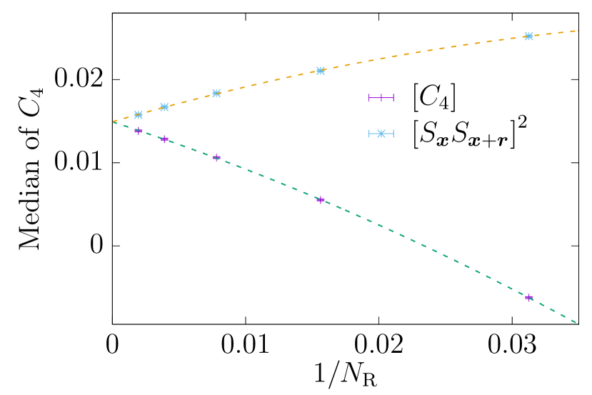
Figure 8: Biased estimators of the median, see (39) and (B.1), as functions of the inverse number of replicas, ${N_{\mathrm{R}}}$, for $T=0.9$ and $\xi({t_{\mathrm{w}}})=20$. The dashed lines are fits to quadratic functions in order to extrapolate to ${N_{\mathrm{R}}}\rightarrow\infty$ (complete fit statistics are available in Table 2).

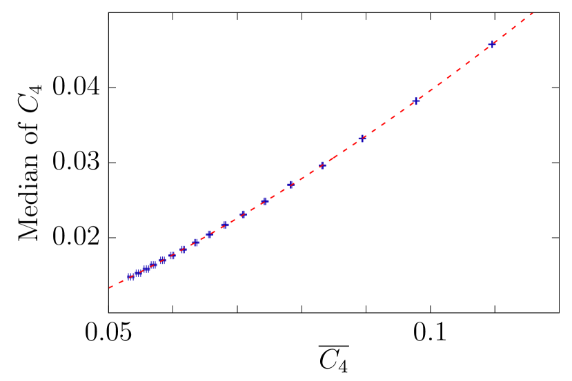
Figure 9: Median of the distribution $P[C_{4}(r=\xi)]$ versus the first moment, $\overline{C_{4}}(r=\xi)$, for $T=0.9$. The median is calculated through the extrapolation to ${N_{\mathrm{R}}}\rightarrow\infty$ shown in Fig. 8. The dashed line is a fit to a power law in order to obtain the slope of $\tau(q)$ near $q=0$ (complete fit information available in Table 2).

B.2 The probability distribution near $C_{4}=1$

As we have shown in the main text, the scaling exponent for the $q$-th moment $\tau(q)$, i.e., $\overline{C_{4}^{q}}\sim 1/[\xi({t_{\mathrm{w}}})]^{\tau(q)}$, goes as $\tau(q)\sim\log q$ for large $q$. This is to be expected if the probability distribution function for $C_{4}$ near 1 behaves as

$$P(C_{4}\to 1)\propto(1-C_{4})^{B(\xi)}\,,$$ (43)

with an exponent $B(\xi)$ that grows logarithmically with $\xi$. Indeed, a simple saddle-point estimation yields

$$\overline{C_{4}^{q}} = \int_{0}^{1}\mathrm{d}C_{4}\,P(C_{4})C_{4}^{q}$$

$$\sim \int_{0}^{1}\mathrm{d}C_{4}\,\exp{[B(\log(1-C_{4})+q\log C_{4}]}\approx\frac{1}{q^{B}}\,.$$

Hence, if $B(\xi)\sim A\log(\xi)$ ($A$ is an amplitude)

$$\frac{1}{q^{A\log\xi}}=\frac{1}{\xi^{A\log q}}\,.$$ (45)

Equipped with the above intuition, we have checked the $P(C_{4}\to 1)$ as computed from the ${N_{\mathrm{R}}}=512$ estimator in (B.1). We obtain a good fit to $(1-C_{4})^{B(\xi)}$, but the determination of the exponent $B(\xi)$ is quite difficult, as it depends significantly on the fitting range. This is why we have turned to a different strategy. We have considered the following expectation value

$${\cal I}({N_{\mathrm{R}}})=\sum_{n={N_{\mathrm{R}}}/2}^{{N_{\mathrm{R}}}}{\cal P}_{s}(n;{N_{\mathrm{R}}},\xi)\mathrm{e}^{-4({N_{\mathrm{R}}}-n)}\,.$$ (46)

The above sum is clearly dominated by values of $n$ near ${N_{\mathrm{R}}}$ where, recall (39), $C_{4}\approx 1-4({N_{\mathrm{R}}}-n)/{N_{\mathrm{R}}}$. Hence, we can approximate

$${\cal I}({N_{\mathrm{R}}}) \approx \int_{0}^{1}\!\mathrm{d}C_{4}\,P(C_{4})\mathrm{e}^{-{N_{\mathrm{R}}}(1-C_{4})}$$

$$\sim \!\int_{0}^{1}\!\mathrm{d}C_{4}\,(1-C_{4})^{B(\xi)}\mathrm{e}^{-{N_{\mathrm{R}}}(1-C_{4})}\sim\frac{1}{{N_{\mathrm{R}}}^{1+B(\xi)}}\,.$$

Then, our chosen strategy has been to fit our data for ${\cal I}({N_{\mathrm{R}}})$ as a power law in $1/{N_{\mathrm{R}}}$, see Fig. 10. Generally speaking, we obtain fair fits (although for $\xi<10$ we had to discard the ${N_{\mathrm{R}}}=32$ data from the fits). The resulting exponents $B(\xi)$ are shown in Fig. 11. As it can be checked, the hypothesis $B(\xi)\propto\log(\xi)$ is tenable, particularly for $\xi>10$.

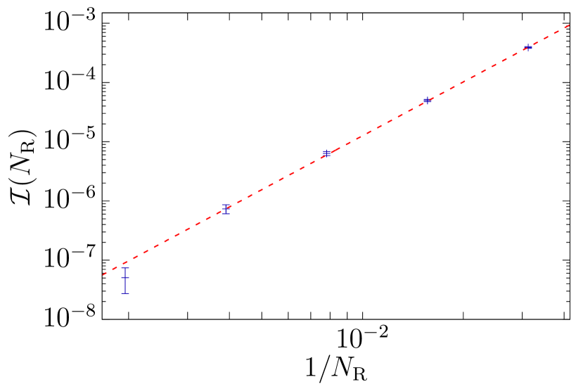
Figure 10: Expectation value ${\cal I}({N_{\mathrm{R}}})$, see  (46), versus the inverse of the number of replicas ${N_{\mathrm{R}}}$, at $T=0.9$ and $\xi({t_{\mathrm{w}}})=20$. The dashed line is a fit to (B.2) with ${N_{\mathrm{R}}}\in[64,512]$ (full details of the fit available in Table 2).

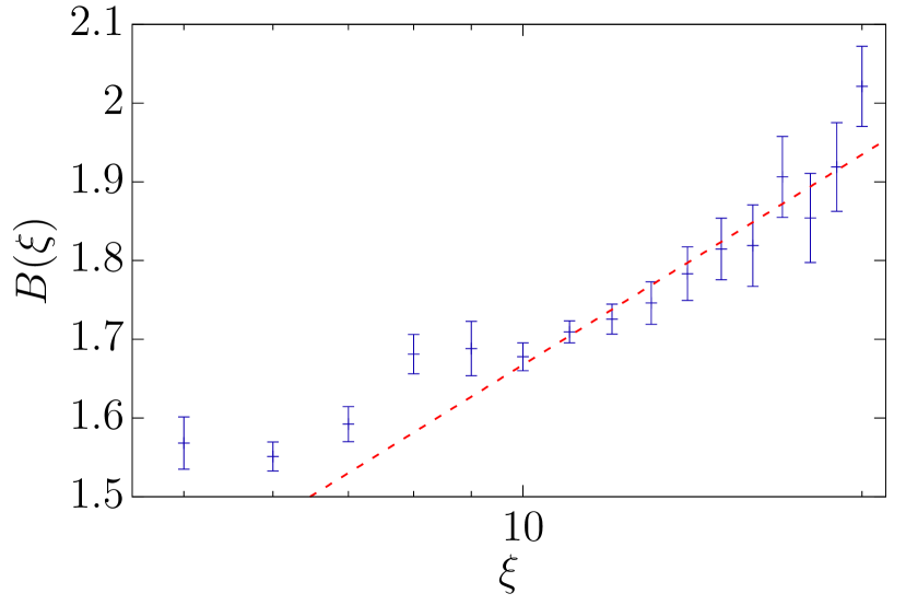
Figure 11: Exponent $B(\xi)$ for $T=0.9$. The dashed line is a fit to $a+b\log(\xi)$ for $\xi\geq 10$ (see Table 2 for complete fit statistics). These results make more plausible a logarithmic behavior of $\tau(q)$ for large $q$.

Appendix C The $\tau(q)$ at $T_{\mathrm{c}}$

We have fitted our data for $\tau(q)$ following the same functional forms that we used at $T=0.9$, namely:

$$\tau_{1}(q)=mq\frac{1+c_{1}q}{1+c_{2}q}\,,\quad\tau_{2}(q)=mq\frac{1+d_{1}q\log q}{(1+d_{2}q)^{2}}\,.$$ (48)

Both $\tau_{1}$ and $\tau_{2}$ have the same derivative at $q\!=\!0$, namely $m$. We do not regard $m$ as a fitting parameter. Rather we take it from the scaling of the median of the distribution $P(C_{4})$ with $\xi$. As usual, we first fitted the median as a function of $\overline{C_{4}}$, see Fig. 9, and then translated it to a power law in $\xi$.

Fig. 12 shows our estimations and fits for $\tau(q)$ for $T=0.9$ and $T=T_{\mathrm{c}}$. Although the functional behaviors of both curves are similar, the clear difference reveals the significantly different nature of the multifractal behaviors at the critical points and in the spin-glass phase.

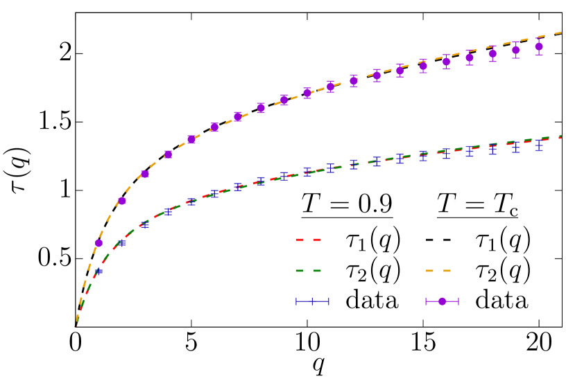
Figure 12: The scaling exponent for the $q$-th moment $\tau(q)$, i.e., $\overline{C_{4}^{q}}\sim 1/[\xi({t_{\mathrm{w}}})]^{\tau(q)}$ versus $q$, as computed for our simulations of the Ising spin glass at $T_{\mathrm{c}}=1.1019(29)$ Baity-Jesi et al. (2013) and $T=0.9$. The dashed lines are fits to the functional forms in (48). Full fit results are shown in Table 2.

Appendix D Summary of the statistical information fits

As stated in the main text, and in the above sections, in order to compute and interpolate $\tau(q)$, and its errors (see Yllanes, 2011), we need to make a huge number of fits. For example, to obtain the data shown in Fig. 9, we need to extrapolate to ${N_{\mathrm{R}}}\rightarrow\infty$ the median of $C_{4}$, see Fig. 8, 16 times at each $\xi({t_{\mathrm{w}}})$ in order to estimate errors. This process would be impossible without some automation. To achieve this, we use a nonlinear least-squares method using the Levenberg-Marquardt solver Levenberg (1944) routine available at the GNU Scientific Library. However, in order to calibrate the process and obtain a fair fits, we perform manually all the fits shown in the present work. The complete statistical information of the fits is summarized in Table 2.

Fig. 13, which shows the evolution of the 10th and 20th moments of $C_{4}$ as function of the coherence length, includes a fit to a power law $a_{q}\xi^{-\tau(q)}$ , where the only parameter is the amplitude constant, $a_{q}$, and the respective value of $\tau(q)$ is the result of our analysis. These fits, included in Table 2, are a good confirmation of our analysis.

D.1 Interpolations necessary to Fig. 4 in the main text

Finally, let us recall that Fig. 4 in the main text requires the evaluation of $C_{4}^{\text{av}}(r,{t_{\mathrm{w}}})$ at non-integer values of its argument. Here, we shall address only the interpolation for our data for the spin glass at $T=0.9$ and ${t_{\mathrm{w}}}$ such that $\xi({t_{\mathrm{w}}})=20$.

In order to interpolate our data, obtained for integer $r$, we have performed a fit that should account for both the short- and long-distance behavior of the correlations:

$$C_{4}^{\text{av}}(r,{t_{\mathrm{w}}}) = F_{\text{sd}}(r)\ +\ F_{\text{ld}}(r)\,,$$

$$F_{\text{sd}}(r) = (b_{0}+b_{1}r+b_{2}r^{2})\mathrm{e}^{-(r/2.6)^{4}}\,,$$ (49)

$$F_{\text{ld}}(r) = \frac{A}{r^{\alpha}}\mathrm{e}^{-(r/\xi_{\text{exp}})^{\beta}}\,.$$

While the functional form for $F_{\text{ld}}(r)$ is well known and physically motivated Belletti et al. (2008b, 2009); Baity-Jesi et al. (2018), we regard $F_{\text{sd}}(r)$ as a purely ad-hoc fitting device. The above functional form fits our integer-$r$ data (within errors) for all $r\geq 1$. Of course, the fitting function can be evaluated whether the argument is integer or not. The fit’s figure of merit is $\chi^{2}/\mathrm{dof}=9.18/71$ ($\mathrm{dof}$ stands for ‘degrees of freedom‘), where we have considered only the diagonal part of the covariance matrix. This partly explains the exceedingly small value of $\chi^{2}$ that we obtained in the fit (the departure of the $p$-value from one is $\sim 10^{-18}$). In order to compute $\chi^{2}$, we considered as well the first image at $L-r$ Fernández et al. (2019), i.e., we compared the numerical data to $f_{\text{sd}}(r)+f_{\text{sd}}(L-r)+f_{\text{ld}}(r)+f_{\text{ld}}(L-r)$.

We conclude this paragraph with the fit parameters (we report many digits for the sake of reproducibility). For the short-distance piece we have:

$$b_{0} = 0.0453360389027432\,,$$

$$b_{1} = -0.0264096080489446\,,$$ (50)

$$b_{2} = 0.00558776268187863\,.$$

The parameters of the long-term decay are:

$$\alpha = 0.45829\,,\quad\beta=1.41217\,,$$ (51)

$$A = 0.551495\,,\quad\xi_{\text{exp}}=20.5207\,.$$

D.2 Comparisons between the diluted ferromagnet and the spin glass

As explained in the main text, both the diluted ferromagnetic Ising model and the spin glass display domain-growth dynamics in their low-temperature phases. In both cases, the size of the domains can be characterized through a coherence length $\xi({t_{\mathrm{w}}})$, see Fig. 14. However, while the spin-glass correlation function at distances $r=\xi$ shows strong statistical fluctuations, see Fig. 15—bottom, this is not the case for the diluted ferromagnet Fig. 15—top. Indeed, for the diluted ferromagnet we see from the figure that $\overline{C_{4}^{2}}/\overline{C_{4}}^{2}$ quickly reaches a finite limit as $\xi({t_{\mathrm{w}}})$ grows. Instead, a steady increase of the ratio $\overline{C_{4}^{2}}/\overline{C_{4}}^{2}$ is observed for the spin glass.

Identifier	Functional Form	Fitting Range	$\chi^{2}/\mathrm{dof}$	Parameters
$[C_{4}]$, Fig. 8	$f(x)=a+bx+cx^{2}$	${N_{\mathrm{R}}}\in[32,512]$	$0.872768/2$	$a=0.01492(12),\ b=-0.52(2),\ c=-5.0(6)$
$[S_{{\bm{x}}}S_{{\bm{x}}+{\bm{r}}}]^{2}$, Fig. 8			$0.946227/2$	$a=0.01492(12),\ b=0.46(2),\ c=-4.3(6)$
${\cal I}({N_{\mathrm{R}}})$, Fig. 10	$f(x)=ax^{(b+1)}$		$3.70448/3$	$a=14(2)$, $b=2.02(4)$
$B(\xi)$, Fig. 11	$f(x)=a+b\log x$	$\xi\in[10,20]$	$5.95738/9$	$a=0.78(11)$, $b=0.39(4)$
$\overline{C_{4}^{q=10}}$, Fig. 13	$f(x)=ax^{-\tau(q)}$		$5.6406/10$	$a=0.00513(2)$
$\overline{C_{4}^{q=20}}$, Fig. 13			$7.64613/10$	$a=0.001337(11)$
Median of $C_{4}$, Fig. 9	$f(x)=ax^{b}$	$\overline{C_{4}}(\xi\in[4,20])$	$1.86484/15$	$a=1.489(16)$, $b=1.575(4)$
$\text{median}[C_{4}]/\overline{C_{4}}$, Fig. 5		$\overline{C_{4}}(\xi\in[4,20])$	$8.88094/15$	$a=1.488(7)$, $b=0.575(2)$
$C_{4}^{\text{av}}(r=\xi;T=0.9)$, Fig. 2		$\xi\in[10,20]$	$1.99859/9$	$a=0.182(2)$, $b=-0.411(5)$
$\tau_{1}(q)$ for $T=0.9$, Fig. 5 and Fig. 12	$f(x)=mx\frac{1+ax}{1+bx}$	$q\in[1,20]$	$5.01227/18$	$a=0.0129(18)$, $b=0.547(12)$
$\tau_{1}(q)$ for $T=T_{\mathrm{c}}$, Fig. 12			$5.37753/18$	$a=0.1718(17)$, $b=0.574(10)$
$\tau_{2}(q)$ for $T=0.9$, Fig. 5 and Fig. 12	$f(x)=mx\frac{1+ax}{(1+bx)^{2}}$		$9.33556/18$	$a=0.039(2)$, $b=0.232(5)$
$\tau_{2}(q)$ for $T=T_{\mathrm{c}}$, Fig. 12			$8.23336/18$	$a=0.0446(2)$, $b=0.242(4)$

Table 2: Summary of the statistical information of all the fits reported in our work. The fits has been done with GNUplot. We have used this data in order to calibrate our analysis, which has been automated to estimate the errors following the strategy of Yllanes (2011).

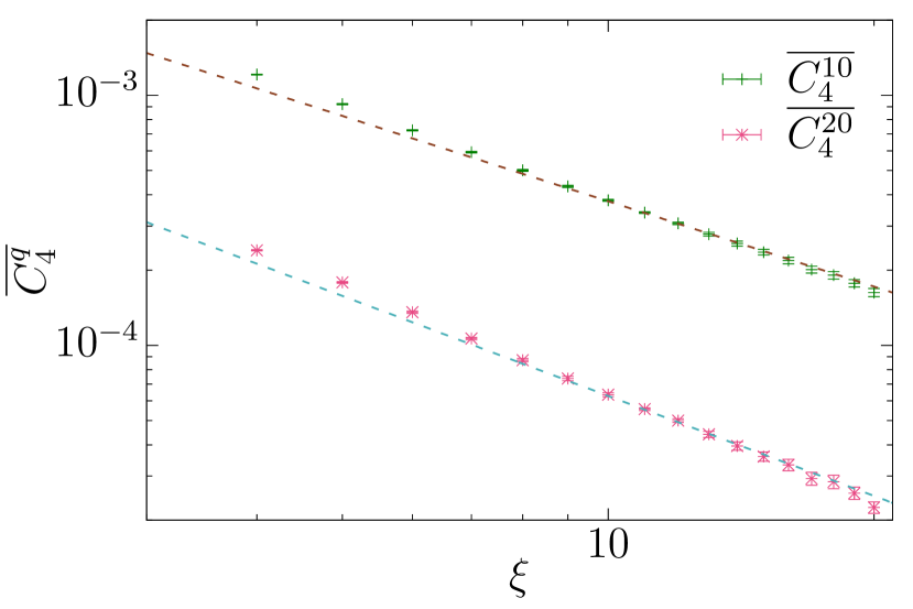
Figure 13: The 10th and 20th moments of $C_{4}$ as functions of the coherence length $\xi$ at $T=0.9$. Dashed lines are fits to $a\xi^{-\tau(q)}$ where the only fitting parameter is the proportionality constant $a$ (fit details are available in Table 2). The values of $\tau(q=10)$, and $\tau(q=20)$ are our final estimates presented in Fig. 12. These fits can be considered as a test of our analysis, showing that our final estimate of $\tau(q)$ is accurate.

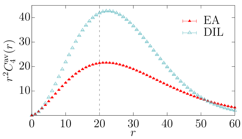
Figure 14: Correlation function $C_{4}^{\text{av}}(r,{t_{\mathrm{w}}})$ multiplied by $r^{2}$, as computed for the three-dimensional Ising diluted ferromagnet (DIL) and for the Ising spin glass (EA), versus distance $r$. Data were obtained in systems of linear size $L=160$ with coherence length $\xi({t_{\mathrm{w}}})=20$ (dashed vertical line) at temperature $T=0.9$—recall that $T_{\mathrm{c}}\approx 1.1$ for the spin glass Baity-Jesi et al. (2013). As explained in Methods in the main text, the coherence length is computed from the integral $I_{2}=\int_{0}^{\infty}r^{2}C^{\text{av}}_{4}(r,{t_{\mathrm{w}}})\mathrm{d}r$. For both models, $r^{2}C^{\text{av}}_{4}(r)$ peaks near $\xi({t_{\mathrm{w}}})$.

Figure 15: Ratio of the second moment of the spin-glass correlation function $C_{4}$ computed at $r=\xi({t_{\mathrm{w}}})$, $\overline{C_{4}^{2}}$, to the squared first moment, $\overline{C_{4}}^{2}$, as a function of the coherence length $\xi({t_{\mathrm{w}}})$. Data computed for the Ising diluted ferromagnet (top) and for Ising spin glass (bottom) at temperatures $T,\ \tilde{T}=0.9,0.8$ and $0.7$ (remember that $T^{\mathrm{DIL}}=\tilde{T}\,(T_{\mathrm{c}}^{\mathrm{DIL}}/T_{\mathrm{c}})$. Error bars are smaller than the point size. Note that, while the diluted ferromagnet tends to one for large coherence length, the spin glass follows a power law, which indicates that in the scaling limit (i.e., $\xi({t_{\mathrm{w}}})\rightarrow\infty$) the order of magnitude of $\overline{C_{4}^{2}}$ is larger than that of $\overline{C_{4}}^{2}$.

References

- Frisch and Parisi (1985) U. Frisch and G. Parisi, in Turbulence and predictability in geophysical fluid dynamics and climate dynamics (1983 International School of Physics ”Enrico Fermi”, Varenna), edited by M. Ghil, R. Benzi, and G. Parisi (North-Holland, Amsterdam, 1985).
- Harte (2001) D. Harte, Multifractals. Theory and applications, 1st ed. (Chapman and Hall/CRC, New York, 2001).
- Wilson (1979) K. G. Wilson, Scientific American 241, 158 (1979).
- Parisi (1988) G. Parisi, Statistical Field Theory (Addison-Wesley, 1988).
- Barnsley (2012) M. Barnsley, Fractals Everywhere, 3rd ed. (Dover Publications Inc., Mineola, New York, 2012).
- Benzi et al. (1984) R. Benzi, G. Paladin, G. Parisi, and A. Vulpiani, Journal of Physics A: Mathematical and General 17, 3521 (1984).
- Castellani and Peliti (1986) C. Castellani and L. Peliti, Journal of physics A: mathematical and general 19, L429 (1986).
- Stanley and Meakin (1988) H. E. Stanley and P. Meakin, Nature 335, 405 (1988).
- Halsey et al. (1986a) T. C. Halsey, M. H. Jensen, L. P. Kadanoff, I. Procaccia, and B. I. Shraiman, Phys. Rev. A 33, 1141 (1986a).
- Halsey et al. (1986b) T. C. Halsey, M. H. Jensen, L. P. Kadanoff, I. Procaccia, and B. I. Shraiman, Phys. Rev. A 34, 1601 (1986b).
- Barabási and Stanley (2009) A.-L. Barabási and H. E. Stanley, Fractal Concepts in Surface Growth (Cambridge University Press, New York, 2009).
- Ivanov et al. (1999) P. C. Ivanov, L. A. N. Amaral, A. L. H. Goldberger, M. G. Shlomo Rosenblum, Z. R. Struzik, and H. E. Stanley, Nature 399, 461 (1999).
- Seuront and Stanley (2014) L. Seuront and H. E. Stanley, Proceedings of the National Academy of Sciences 111, 2206 (2014).
- Klopper (2014) A. Klopper, Nature Physics 10, 183 (2014).
- Deidda (2000) R. Deidda, Water Resources Research 36, 1779 (2000).
- Alvarez-Ramirez et al. (2008) J. Alvarez-Ramirez, J. Alvarez, and E. Rodriguez, Energy Economics 30, 2645 (2008).
- Mydosh (1993) J. A. Mydosh, Spin Glasses: an Experimental Introduction (Taylor and Francis, London, 1993).
- Charbonneau et al. (2023) P. Charbonneau, E. Marinari, M. Mézard, G. Parisi, F. Ricci-Tersenghi, G. Sicuro, and F. Zamponi, Spin Glass Theory and Far Beyond (WORLD SCIENTIFIC, 2023) https://www.worldscientific.com/doi/pdf/10.1142/13341 .
- Vincent et al. (1997) E. Vincent, J. Hammann, M. Ocio, J.-P. Bouchaud, and L. F. Cugliandolo, in Complex Behavior of Glassy Systems, Lecture Notes in Physics No. 492, edited by M. Rubí and C. Pérez-Vicente (Springer, 1997).
- Zhai et al. (2019) Q. Zhai, V. Martin-Mayor, D. L. Schlagel, G. G. Kenning, and R. L. Orbach, Phys. Rev. B 100, 094202 (2019).
- Zhai et al. (2020) Q. Zhai, I. Paga, M. Baity-Jesi, E. Calore, A. Cruz, L. A. Fernandez, J. M. Gil-Narvion, I. Gonzalez-Adalid Pemartin, A. Gordillo-Guerrero, D. Iñiguez, A. Maiorano, E. Marinari, V. Martin-Mayor, J. Moreno-Gordo, A. Muñoz Sudupe, D. Navarro, R. L. Orbach, G. Parisi, S. Perez-Gaviro, F. Ricci-Tersenghi, J. J. Ruiz-Lorenzo, S. F. Schifano, D. L. Schlagel, B. Seoane, A. Tarancon, R. Tripiccione, and D. Yllanes, Phys. Rev. Lett. 125, 237202 (2020).
- Paga et al. (2021) I. Paga, Q. Zhai, M. Baity-Jesi, E. Calore, A. Cruz, L. A. Fernandez, J. M. Gil-Narvion, I. Gonzalez-Adalid Pemartin, A. Gordillo-Guerrero, D. Iñiguez, A. Maiorano, E. Marinari, V. Martin-Mayor, J. Moreno-Gordo, A. Muñoz-Sudupe, D. Navarro, R. L. Orbach, G. Parisi, S. Perez-Gaviro, F. Ricci-Tersenghi, J. J. Ruiz-Lorenzo, S. F. Schifano, D. L. Schlagel, B. Seoane, A. Tarancon, R. Tripiccione, and D. Yllanes, Journal of Statistical Mechanics: Theory and Experiment 2021, 033301 (2021).
- Zhai et al. (2022) Q. Zhai, R. L. Orbach, and D. L. Schlagel, Phys. Rev. B 105, 014434 (2022).
- Belletti et al. (2008a) F. Belletti, M. Cotallo, A. Cruz, L. A. Fernandez, A. Gordillo, A. Maiorano, F. Mantovani, E. Marinari, V. Martín-Mayor, A. Muñoz Sudupe, D. Navarro, S. Perez-Gaviro, J. J. Ruiz-Lorenzo, S. F. Schifano, D. Sciretti, A. Tarancon, R. Tripiccione, and J. L. Velasco (Janus Collaboration), Comp. Phys. Comm. 178, 208 (2008a), arXiv:0704.3573 .
- Baity-Jesi et al. (2017) M. Baity-Jesi, E. Calore, A. Cruz, L. A. Fernandez, J. M. Gil-Narvión, A. Gordillo-Guerrero, D. Iñiguez, A. Maiorano, E. Marinari, V. Martin-Mayor, J. Monforte-Garcia, A. Muñoz Sudupe, D. Navarro, G. Parisi, S. Perez-Gaviro, F. Ricci-Tersenghi, J. J. Ruiz-Lorenzo, S. F. Schifano, B. Seoane, A. Tarancón, R. Tripiccione, and D. Yllanes, Proceedings of the National Academy of Sciences 114, 1838 (2017).
- Baity-Jesi et al. (2018) M. Baity-Jesi, E. Calore, A. Cruz, L. A. Fernandez, J. M. Gil-Narvion, A. Gordillo-Guerrero, D. Iñiguez, A. Maiorano, E. Marinari, V. Martin-Mayor, J. Moreno-Gordo, A. Muñoz Sudupe, D. Navarro, G. Parisi, S. Perez-Gaviro, F. Ricci-Tersenghi, J. J. Ruiz-Lorenzo, S. F. Schifano, B. Seoane, A. Tarancon, R. Tripiccione, and D. Yllanes (Janus Collaboration), Phys. Rev. Lett. 120, 267203 (2018).
- Baity-Jesi et al. (2023) M. Baity-Jesi, E. Calore, A. Cruz, L. A. Fernandez, J. M. Gil-Narvion, I. Gonzalez-Adalid Pemartin, A. Gordillo-Guerrero, D. Iñiguez, A. Maiorano, E. Marinari, V. Martin-Mayor, J. Moreno-Gordo, A. Muñoz Sudupe, D. Navarro, I. Paga, G. Parisi, S. Perez-Gaviro, F. Ricci-Tersenghi, J. J. Ruiz-Lorenzo, S. F. Schifano, B. Seoane, A. Tarancon, and D. Yllanes, Nature Physics 19, 978 (2023).
- Jonason et al. (1998) K. Jonason, E. Vincent, J. Hammann, J. P. Bouchaud, and P. Nordblad, Phys. Rev. Lett. 81, 3243 (1998).
- Baity-Jesi et al. (2021) M. Baity-Jesi, E. Calore, A. Cruz, L. A. Fernandez, J. M. Gil-Narvion, I. Gonzalez-Adalid Pemartin, A. Gordillo-Guerrero, D. Iñiguez, A. Maiorano, E. Marinari, V. Martin-Mayor, J. Moreno-Gordo, A. Muñoz Sudupe, D. Navarro, I. Paga, G. Parisi, S. Perez-Gaviro, F. Ricci-Tersenghi, J. J. Ruiz-Lorenzo, S. F. Schifano, B. Seoane, A. Tarancon, R. Tripiccione, and D. Yllanes, Communications physics 4, 74 (2021), https://www.nature.com/articles/s42005-021-00565-9.pdf .
- Baity-Jesi et al. (2014a) M. Baity-Jesi, R. A. Baños, A. Cruz, L. A. Fernandez, J. M. Gil-Narvion, A. Gordillo-Guerrero, D. Iniguez, A. Maiorano, F. Mantovani, E. Marinari, V. Martín-Mayor, J. Monforte-Garcia, A. Muñoz Sudupe, D. Navarro, G. Parisi, S. Perez-Gaviro, M. Pivanti, F. Ricci-Tersenghi, J. J. Ruiz-Lorenzo, S. F. Schifano, B. Seoane, A. Tarancon, R. Tripiccione, and D. Yllanes (Janus Collaboration), Comp. Phys. Comm 185, 550 (2014a), arXiv:1310.1032 .
- Baity-Jesi et al. (2013) M. Baity-Jesi, R. A. Baños, A. Cruz, L. A. Fernandez, J. M. Gil-Narvion, A. Gordillo-Guerrero, D. Iniguez, A. Maiorano, F. Mantovani, E. Marinari, V. Martín-Mayor, J. Monforte-Garcia, A. Muñoz Sudupe, D. Navarro, G. Parisi, S. Perez-Gaviro, M. Pivanti, F. Ricci-Tersenghi, J. J. Ruiz-Lorenzo, S. F. Schifano, B. Seoane, A. Tarancon, R. Tripiccione, and D. Yllanes (Janus Collaboration), Phys. Rev. B 88, 224416 (2013), arXiv:1310.2910 .
- Note (1) At its critical temperature, the two-dimensional diluted ferromagnetic Potts model with more than two states presents multiscaling as well Ludwig (1990) —this is also the case for the diluted Ising model in Davis and Cardy (2000); Marinari et al. (2023).
- Note (2) The droplet picture of spin glasses McMillan (1983); Bray and Moore (1978); Fisher and Huse (1986) predicts , similarly to the ferromagnet. Neither simulations nor experimental data are compatible with , unless one is willing to accept that the available range of is too small to display the true asymptotic behavior Baity-Jesi et al. (2018).
- Benzi et al. (1993) R. Benzi, S. Ciliberto, R. Tripiccione, C. Baudet, F. Massaioli, and S. Succi, Phys. Rev. E 48, R29 (1993).
- Chen and Lubensky (1977) J.-H. Chen and T. C. Lubensky, Phys. Rev. B 16, 2106 (1977).
- De Dominicis and Kondor (1989) C. De Dominicis and I. Kondor, Journal of Physics A: Mathematical and General 22, L743 (1989).
- Note (3) The correlation function behaves as for large , where the cut-off function decays faster than exponentially as grows [see, e.g., Refs. Belletti et al. (2008b); Fernández et al. (2019)]. Hence, for one may consider either power-law scaling in —as in (1)— or in —as in (2). The analysis of scale invariance in a fractal (or multifractal) geometry typically involves power laws.
- Baity-Jesi et al. (2014b) M. Baity-Jesi, R. A. Baños, A. Cruz, L. A. Fernandez, J. M. Gil-Narvion, A. Gordillo-Guerrero, D. Iniguez, A. Maiorano, M. F., E. Marinari, V. Martín-Mayor, J. Monforte-Garcia, A. Muñoz Sudupe, D. Navarro, G. Parisi, S. Perez-Gaviro, M. Pivanti, F. Ricci-Tersenghi, J. J. Ruiz-Lorenzo, S. F. Schifano, B. Seoane, A. Tarancon, R. Tripiccione, and D. Yllanes, J. Stat. Mech. 2014, P05014 (2014b), arXiv:1403.2622 .
- Franz et al. (1998) S. Franz, M. Mézard, G. Parisi, and L. Peliti, Phys. Rev. Lett. 81, 1758 (1998).
- Alvarez Baños et al. (2010) R. Alvarez Baños, A. Cruz, L. A. Fernandez, J. M. Gil-Narvion, A. Gordillo-Guerrero, M. Guidetti, A. Maiorano, F. Mantovani, E. Marinari, V. Martín-Mayor, J. Monforte-Garcia, A. Muñoz Sudupe, D. Navarro, G. Parisi, S. Perez-Gaviro, J. J. Ruiz-Lorenzo, S. F. Schifano, B. Seoane, A. Tarancon, R. Tripiccione, and D. Yllanes (Janus Collaboration), Phys. Rev. Lett. 105, 177202 (2010), arXiv:1003.2943 .
- Wittmann and Young (2016) M. Wittmann and A. P. Young, Journal of Statistical Mechanics: Theory and Experiment 2016, 013301 (2016).
- Jensen et al. (2021) S. Jensen, N. Read, and A. P. Young, Phys. Rev. E 104, 034105 (2021).
- Amit and Martín-Mayor (2005) D. J. Amit and V. Martín-Mayor, Field Theory, the Renormalization Group and Critical Phenomena, 3rd ed. (World Scientific, Singapore, 2005).
- Yllanes (2011) D. Yllanes, Rugged Free-Energy Landscapes in Disordered Spin Systems, Ph.D. thesis, Universidad Complutense de Madrid (2011), arXiv:1111.0266 .
- Belletti et al. (2008b) F. Belletti, M. Cotallo, A. Cruz, L. A. Fernandez, A. Gordillo-Guerrero, M. Guidetti, A. Maiorano, F. Mantovani, E. Marinari, V. Martín-Mayor, A. M. Sudupe, D. Navarro, G. Parisi, S. Perez-Gaviro, J. J. Ruiz-Lorenzo, S. F. Schifano, D. Sciretti, A. Tarancon, R. Tripiccione, J. L. Velasco, and D. Yllanes (Janus Collaboration), Phys. Rev. Lett. 101, 157201 (2008b), arXiv:0804.1471 .
- Belletti et al. (2009) F. Belletti, A. Cruz, L. A. Fernandez, A. Gordillo-Guerrero, M. Guidetti, A. Maiorano, F. Mantovani, E. Marinari, V. Martín-Mayor, J. Monforte, A. Muñoz Sudupe, D. Navarro, G. Parisi, S. Perez-Gaviro, J. J. Ruiz-Lorenzo, S. F. Schifano, D. Sciretti, A. Tarancon, R. Tripiccione, and D. Yllanes (Janus Collaboration), J. Stat. Phys. 135, 1121 (2009), arXiv:0811.2864 .
- Berche et al. (2004) P.-E. Berche, C. Chatelain, B. Berche, and W. Janke, The European Physical Journal B - Condensed Matter and Complex Systems 38, 463 (2004).
- Note (4) Recall that we set times such that .
- Levenberg (1944) K. Levenberg, Quarterly of Applied Mathematics 2, 164 (1944).
- Fernández et al. (2019) L. A. Fernández, E. Marinari, V. Martín-Mayor, G. Parisi, and J. Ruiz-Lorenzo, Journal of Physics A: Mathematical and Theoretical 52, 224002 (2019).
- Ludwig (1990) A. W. W. Ludwig, Nucl. Phys. B 330, 639 (1990).
- Davis and Cardy (2000) T. Davis and J. Cardy, Nuclear Physics B 570, 713 (2000).
- Marinari et al. (2023) E. Marinari, , V. Martín-Mayor, G. Parisi, F. Ricci-Tersenghi, and J. J. Ruiz-Lorenzo, “Multiscaling in the critical site-diluted ferromagnet,” (2023), manuscript in preparation.
- McMillan (1983) W. L. McMillan, Phys. Rev. B 28, 5216 (1983).
- Bray and Moore (1978) A. J. Bray and M. A. Moore, Phys. Rev. Lett. 41, 1068 (1978).
- Fisher and Huse (1986) D. S. Fisher and D. A. Huse, Phys. Rev. Lett. 56, 1601 (1986).