Gravito-thermal transports, Onsager reciprocal relation and gravitational Wiedemann-Franz law

Abstract

Using the near-detailed-balance distribution function obtained in our recent work, we present a set of covariant gravito-thermal transport equations for neutral relativistic gases in a generic stationary spacetime. All relevant tensorial transport coefficients are worked out and are presented using some particular integration functions in $(\alpha,\zeta)$, where $\alpha=-\beta\mu$ and $\zeta=\beta m$ is the relativistic coldness, with $\beta$ being the inverse temperature and $\mu$ being the chemical potential. It is shown that the Onsager reciprocal relation holds in the gravito-thermal transport phenomena, and that the heat conductivity and the gravito-conductivity tensors are proportional to each other, with the coefficient of proportionality given by the product of the so-called Lorenz number with the temperature, thus proving a gravitational variant of the Wiedemann-Franz law. It is remarkable that, for strongly degenerate Fermi gases, the Lorenz number takes a universal constant value $L=\pi^{2}/3$, which extends the Wiedemann-Franz law into the Wiedemann-Franz-Lorenz law.

1 Introduction

A salient feature of thermodynamics is that of universality. Different systems can have similar qualitative macroscopic behaviors irrespective of the microscopic structures. This feature is especially manifest for systems under equilibrium. Beyond that, in the case when slight departures from global equilibrium appear, it is common for all fluid systems to share similar phenomenological transport laws and heavy emphasis was placed on the general symmetry principle that restricts the kinetic coefficients, namely the Onsager reciprocal relation [1, 2].

Historically, a great deal of efforts have been devoted to the unveiling of universality in irreversible processes, and the general framework develops over long periods of time until various empirical relations can be reformulated using the methods from statistical mechanics [3, 4]. However, in this pattern, attention has rarely been paid to the transport phenomena controlled fully by relativistic gravitational field. The reason for such a situation stems from the fact that, on one hand, in laboratory condensed matter experiments, gravity is too weak to play a key role, on the other hand, the relativistic statistical mechanics is far from being established.

Over the past few years, with the abundant data accumulated by the LIGO/Virgo gravitational wave detectors [5] and the Event Horizon Telescope [6], physics in strong gravity becomes ready to merit broader attentions. This new era of fundamental physics and astronomy calls for an extension of thermodynamics and statistical mechanics to strong gravity regime. On the theoretical side, a statistical mechanical explanation of black hole thermodynamics is expected to contribute insight into quantum gravity [7, 8]. For the observational studies, the brightest sources in the universe are powered black holes, where the temperature of the near-horizon environment reaches $10^{9}$ K and much of the gravitational potential energy is converted into heat, which is in turn carried away by radiation [9]. To this end, it becomes increasingly important to provide additional understanding about the thermodynamic behaviors of the relativistic gases that are flowing around black holes. The aim of the present work is to study the transport phenomena of relativistic gases subjecting to strong gravity.

The earliest investigation about gravito-thermal effects was carried out by Tolman and Ehrenfest [10, 11], who noticed a remarkable feature of gravity. Building on the idea that heat — as a form of energy — should also gravitate, they argued that the temperature gradient could be compensated for by gravitational field to restore equilibrium, and vice versa. This mechanism is known as the Tolman-Ehrenfest (TE) effect, and since the original outset, both its validity and generality have been extensively studied [12, 13, 14, 15, 16, 17, 18]. The most famous application of the TE effect is in the Luttinger theory of thermal transport coefficients [19], where gravity comes into play as a counter-term for the temperature gradient, which enables the calculation of thermal transport coefficients within the framework of linear response theory. This is the beginning for gravity to appear in condensed-matter physics, and the seminal work of Luttinger has now been generalized to the quantum level, where various new transport effects arise due to anomalies [20]. In all these cases, only weak gravitational field is needed. Please be reminded that there is a parallel effect which applies to the gradient of the chemical potential, known as the Klein effect. Although these gravito-thermal effects are still too weak to be observed directly, the simplest way to unify the description for various transport phenomena is to acknowledge their existence in principle.

Another well-known approach to transport phenomena is kinetic theory [21, 22, 23] which has been successfully generalized in a form that is manifestly covariant, and increasingly applied to the study of quark-gluon plasma [24, 25, 26], cosmology and black hole accretion [27, 28, 29, 30, 31, 32, 33]. Recently in [34], taking advantage of the relativistic Boltzmann equation and an observer dependent collision model, we obtained a covariant transport equation for the particle number flow by collecting the TE effect and Klein effect in the generalized gradients of the temperature and chemical potential, and obtained in analytic form the corresponding tensorial transport coefficients, including the gravito-conductivity tensor as a particular example.

The present paper is a continuation of the previous study [34]. The main purpose is three-folded. Firstly, as further applications of the near-equilibrium solution found in [34], we take a step forward to construct the transport equations for the internal energy and entropy flows and calculate the corresponding transport tensors in covariant form. Due to the fundamental local thermodynamic relation which still holds in systems obeying the local equilibrium assumption, the entropy flow is not independent of the particle number and internal energy flows. Secondly, assembling the transport coefficients for the particle number and internal energy flows together, we verify that the celebrated Onsager reciprocal relation still holds for the kinetic coefficients associated with the gravito-thermal transport phenomena. Lastly, by introducing the heat flow as the internal energy flow in the absence of net particle number flow, we obtain the heat conductivity tensor, which is then verified to be proportional to the gravito-conductivity, with product of the temperature and the so-called Lorenz number playing the role of proportionality factor. This proves a gravitational variant of the Wiedemann-Franz law. The Lorenz number $L$ is described analytically by some expression involving several integration functions, and, interestingly, for strongly degenerate Fermi gases, $L$ takes a universal constant value $\pi^{2}/3$ in both the non-relativistic and ultra-relativistic limits.

2 Thermodynamic forces in gravitational field

This section is a reminder for the basics of conventional non-equilibrium thermodynamics and relativistic kinetic theory. We shall also introduce notations and quantities which are necessary for describing non-equilibrium thermodynamic processes in curved spacetimes.

Non-equilibrium systems contain the flows of particle number and various other quantities (“charges”) driven by thermodynamic forces. For near equilibrium systems, the flows can be viewed as linear responses to the thermodynamic forces, and the response factors are known as transport coefficients. For example, in the absence of particle number flow, Fourier’s law relates the heat flow to temperature gradient; while in the absence of heat flow, Fick’s law describes the relation between particle diffusion and concentration gradient. Non-equilibrium thermodynamics provides us with a basis for understanding these phenomenological laws.

To deal with non-equilibrium systems, the first difficulty arises in defining the entropy. This problem can be solved when the characteristic time of macroscopic evolution is much larger than the timescale for microscopic process but otherwise much smaller than the relaxation time for the system to become equilibrated. In such cases, the local equilibrium assumption could be adopted, which assumes that, although the global fundamental relation of equilibrium thermodynamics is necessarily broken, the local variant in terms of densities should still hold,

$$\mathrm{d}s=\frac{1}{T}\mathrm{d}\epsilon-\frac{\mu}{T}\mathrm{d}n,$$ (1)

where $s$, $\epsilon$ and $n$ respectively represent the local densities of the entropy, internal energy and particle number. The local fundamental relation as presented above is usually referred to as the entropic representation. In this representation, the intensive quantities are known as the Massieu parameters, i.e.

$$\alpha=\frac{\partial s}{\partial n}=-\frac{\mu}{T},\qquad\beta=\frac{\partial s}{\partial\epsilon}=\frac{1}{T},$$

and their gradients are defined as the entropic thermodynamic forces

$$\vec{\mathcal{F}}^{(\alpha)}=\nabla\alpha,\qquad\vec{\mathcal{F}}^{(\beta)}=\nabla\beta.$$ (2)

Later, in the relativistic context, the parameter $\beta$ is often replaced by the dimensionless parameter $\zeta=\beta m$, which is called the relativistic coldness.

In the presence of non-vanishing thermodynamic forces, eq.(1) suggests the following relation between the entropy flow $\vec{j}_{s}$ with the internal energy flow $\vec{j}_{\epsilon}$ and the particle number flow $\vec{j}_{n}$,

$$\vec{j}_{s}=\alpha\vec{j}_{n}+\beta\vec{j}_{\epsilon}.$$ (3)

Consequently, the entropy production rate will be expressed in terms of flows and the thermodynamic forces,

$$\mathcal{G}_{s}=\vec{\mathcal{F}}^{(\alpha)}\cdot\vec{j}_{n}+\vec{\mathcal{F}}^{(\beta)}\cdot\vec{j}_{\epsilon}.$$

To close the above equations, one needs supplementary transport equations relating the flows to thermodynamic forces. A common approach is to expand the flows in powers of the thermodynamic forces, and for near equilibrium systems it is sufficient to restrict the discussion to the linear order. As a result, one has

$$\bm{j}^{a}=\left(\begin{matrix}j^{a}_{n}\\ j^{a}_{\epsilon}\\ \end{matrix}\right)=\left(\begin{matrix}L^{\,ab}_{(\alpha\alpha)}&L^{\,ab}_{(\alpha\beta)}\\ L^{\,ab}_{(\beta\alpha)}&L^{\,ab}_{(\beta\beta)}\\ \end{matrix}\right)\left(\begin{matrix}\mathcal{F}_{b}^{(\alpha)}\\ \mathcal{F}_{b}^{(\beta)}\\ \end{matrix}\right)=\bm{L}^{ab}\bm{\mathcal{F}}_{b}.$$

The components of matrix $\bm{L}^{ab}$ are called kinetic coefficients and they capture the characteristics of non-equilibrium systems in the linear response regime. These kinetic coefficients can be obtained by experiment or by means of non-equilibrium statistical mechanics. Either way, there is an symmetry principle for $\bm{L}^{ab}$. For charged system, and in the presence of external magnetic field $\bm{B}$, the Onsager relation is given by

$$\bm{L}^{ab}\left[\bm{B}\right]=\left(\bm{L}^{\mathrm{T}}\right)^{ba}\left[-\bm{B}\right],$$ (4)

which is of fundamental importance in non-equilibrium thermodynamics.

The above brief picture for non-equilibrium thermodynamics did not take the microscopic description (i.e. statistical physics description) into account, and has nothing to do with gravity. In order to present a statistical description for a neutral relativistic fluid subjecting strong gravity, we employ the relativistic kinetic theory, in which the one particle distribution function (1PDF) $f$ plays a key role. In the following, it is suffices to consider only the primary variables, namely the particle number current $N^{\mu}$, the energy momentum tensor $T^{\mu\nu}$ and the entropy current $S^{\mu}$, for the relativistic fluid. These objects are determined by 1PDF $f$ and the metric tensor $g_{\mu\nu}$ via

$$N^{\mu}=\int\bm{\varpi}p^{\mu}f,\qquad T^{\mu\nu}=\int\bm{\varpi}p^{\mu}p^{\nu}f,$$

$$S^{\mu}=-\int\bm{\varpi}p^{\mu}\left[f\log f-\varsigma^{-1}\left(1+\varsigma f\right)\log\left(1+\varsigma f\right)\right],$$ (5)

where $\bm{\varpi}=\mathfrak{g}\frac{\sqrt{g}}{p_{0}}(\mathrm{d}p)^{d}$ is invariant volume element on the momentum space with $\mathfrak{g}$ being the intrinsic degeneracy factor, and $\varsigma=0,+1,-1$ corresponds respectively to the Maxwell-Boltzmann, Bose-Einstein and Fermi-Dirac statistics. Since the integrations are performed only over the momentum space, $T^{\mu\nu}$, $N^{\nu}$ and $S^{\mu}$ are local quantities in spacetime. Please be reminded that, throughout this paper, we will work in units $k_{\rm B}=c=\hbar=1$ and the convention on the signature of the metric is the mostly positive one.

Strictly speaking, the dynamics of $g_{\mu\nu}$ and $f$ are governed by a set of coupled equations including Einstein equation and Boltzmann equation, but the present work considers only probe systems in a prescribed spacetime background, thus $f$ is to be regarded as the solution to the relativistic Boltzmann equation

$$\pounds_{H}f(x,p)=\mathcal{C}(x,p),$$

where $\pounds_{H}$ represents the Liouville vector field on the tangent bundle over the fixed $(d+1)$-dimensional curved spacetime background, and $\mathcal{C}(x,p)$ represents the collision term.

In fact, an exact treatment of the relativistic Boltzmann equation alone is still perplexing because it is hard to determine the collision term in closed form. In the cases when the collision contribution completely disappears, the Boltzmann equation degenerates into the Liouville equation, and there is a unique solution $\bar{f}$ under the assumptions that the elementary processes are time-reversal invariant and the entropy production rate vanishes. $\bar{f}$ is known as the detailed balance distribution and it takes the form

$$\bar{f}=\frac{1}{\mathrm{e}^{\bar{\alpha}-\bar{\mathcal{B}}_{\mu}p^{\mu}}-\varsigma},$$ (6)

where $\bar{\alpha}$ and $\bar{\mathcal{B}}^{\mu}$ are constrained by

$$\partial_{\mu}\bar{\alpha}=0,\qquad\qquad\nabla_{(\mu}\mathcal{\bar{B}}_{\nu)}=0.$$ (7)

By convention, all “barred” variables refer to quantities describing systems in detailed balance. Notice that the equation obeyed by $\bar{\mathcal{B}}^{\mu}$ is a Killing equation, and in order to have a non-relativistic limit, the expression $-\bar{\mathcal{B}}_{\mu}p^{\mu}$ needs to be proportional to the energy of the particle, and thus requires $\bar{\mathcal{B}}_{\mu}$ to be timelike. Therefore, in order for the detailed balance distribution (7) to exist, $\bar{\mathcal{B}}^{\mu}$ is required to be a timelike Killing vector field, which in turn implies that the spacetime background must be at least stationary.

The primary variables $N^{\mu}$, $T^{\mu\nu}$ and $S^{\mu}$ have phenomenological interpretations. As such, their component forms must be observer dependent. For systems in stationary spacetimes, the common choice for the observers is that of the stationary class, whose proper velocity field $Z^{\mu}$ is proportional to the timelike Killing vector field $\bar{\mathcal{B}}^{\mu}$,

$$\mathcal{\bar{B}}^{\mu}=\bar{\beta}Z^{\mu},\qquad Z^{\mu}Z_{\mu}=-1.$$

In terms of such observers, the primary variables for the relativistic fluid under detailed balance are evaluated to be

$$\begin{split}&\bar{N}^{\mu}=\mathfrak{g}m^{d}\mathcal{A}_{d-1}\bar{J}_{d-1,1}\,Z^{\mu},\\ &\bar{T}^{\mu\nu}=\mathfrak{g}m^{d+1}\mathcal{A}_{d-1}\left(\bar{J}_{d-1,2}\,Z^{\mu}Z^{\nu}+\frac{1}{d}\bar{J}_{d+1,0}\,\Delta^{\mu\nu}\right),\\ &\bar{S}^{\mu}=\mathfrak{g}m^{d}\mathcal{A}_{d-1}\left(\bar{\alpha}\bar{J}_{d-1,1}+\bar{\zeta}\bar{J}_{d-1,2}+\frac{\bar{\zeta}}{d}\bar{J}_{d+1,0}\right)Z^{\mu},\end{split}$$ (8)

where $\mathcal{A}_{d-1}$ is the area of the $(d-1)$-dimensional unit sphere, $m$ is the mass of constituent particles, $\Delta^{\mu\nu}=g^{\mu\nu}+Z^{\mu}Z^{\nu}$ is the projection tensor, and $\bar{J}_{n,m}$ represents the following function in $(\bar{\alpha},\bar{\zeta})$, with $\bar{\zeta}=\bar{\beta}m$,

$$\bar{J}_{n,m}=J_{n,m}(\bar{\alpha},\bar{\zeta},\varsigma),$$

$$J_{n,m}(\alpha,\zeta,\varsigma)\equiv\int_{0}^{\infty}\frac{\sinh^{n}\vartheta\cosh^{m}\vartheta}{\mathrm{e}^{\alpha+\zeta\cosh\vartheta}-\varsigma}\mathrm{d}\vartheta.$$ (9)

The form of eq.(8) implies that the stationary observers are automatically comoving for systems in detailed balance.

From equations (7) and (8) we can conclude that:

i)

In the eyes of stationary observer, the system under detailed balance is completely characterized by the scalar densities $\bar{n}$, $\bar{\epsilon}$ and $\bar{s}$ and the pressure $\bar{P}$, which are all functions in $\bar{\alpha}$ and $\bar{\beta}$,

$$\bar{n} \equiv-Z_{\mu}N^{\mu}=\mathfrak{g}m^{d}\mathcal{A}_{d-1}\bar{J}_{d-1,1},\qquad\quad\qquad\bar{\epsilon}\equiv Z_{\mu}Z_{\nu}T^{\mu\nu}=\mathfrak{g}m^{d+1}\mathcal{A}_{d-1}\bar{J}_{d-1,2},$$

$$\bar{P} \equiv\frac{1}{d}T^{\rho\sigma}\Delta_{\rho}{}^{\mu}\Delta_{\sigma\mu}=\mathfrak{g}m^{d+1}\frac{\mathcal{A}_{d-1}}{d}\bar{J}_{d+1,0},\quad\,\,\bar{s}\equiv-Z_{\mu}S^{\mu}=\bar{\alpha}\bar{n}+\bar{\beta}\bar{\epsilon}+\bar{\beta}\bar{P}.$$

ii)

In differential form, we have the relations

$$\mathrm{d}\bar{s}=\bar{\alpha}\,\mathrm{d}\bar{n}+\bar{\beta}\,\mathrm{d}\bar{\epsilon},\qquad\mathrm{d}\bar{P}=\bar{s}\,\mathrm{d}(\bar{\beta}^{-1})-\bar{n}\,\mathrm{d}(\bar{\alpha}\bar{\beta}^{-1}).$$

Therefore, $\bar{\alpha}$ and $\bar{\beta}$ acquire the interpretation as Massieu parameters under detailed balance,

$$\bar{\alpha}=-\bar{\mu}/\bar{T},\qquad\quad\bar{\beta}=1/\bar{T}.$$

The parameter $\bar{\zeta}=\bar{\beta}m$ then is understood to be the relativistic coldness in detailed balance.

iii)

There is no macroscopic transports in systems under detailed balance. However, the gradients of the temperature and chemical potential can still be nonvanishing,

$$\nabla_{\nu}\bar{T}=-\bar{T}Z^{\sigma}\nabla_{\sigma}Z_{\nu},\qquad\nabla_{\nu}\bar{\mu}=-\bar{\mu}Z^{\sigma}\nabla_{\sigma}Z_{\nu}.$$ (10)

If the right hand sides do not vanish, these gradients can be understood as manifestations of the TE and Klein effects.

In view of the last property, it is proposed in [34] that the gradients of the temperature and chemical potential should be generalized as

$$\mathcal{D}_{\nu}T\equiv\nabla_{\nu}T+TZ^{\sigma}\nabla_{\sigma}Z_{\nu},\qquad\mathcal{D}_{\nu}\mu\equiv\nabla_{\nu}\mu+\mu Z^{\sigma}\nabla_{\sigma}Z_{\nu}.$$

For any function $\Psi$ in $(T,\mu)$, we also introduce the corresponding generalized gradient

$$\mathcal{D}_{\nu}\Psi(T,\mu)=\left(\frac{\partial\Psi}{\partial T}\right)\mathcal{D}_{\nu}T+\left(\frac{\partial\Psi}{\partial\mu}\right)\mathcal{D}_{\nu}\mu,$$ (11)

and define

$$\dot{\Psi}=Z^{\nu}\mathcal{D}_{\nu}\Psi.$$ (12)

Thus the generalized gradients of the Massieu parameters $\alpha$ and $\beta$ are given by

$$\mathcal{D}_{\nu}\alpha=\mathcal{D}_{\nu}\left(-\frac{\mu}{T}\right)=\nabla_{\nu}\alpha,\quad\mathcal{D}_{\nu}\beta=\mathcal{D}_{\nu}\left(\frac{1}{T}\right)=\nabla_{\nu}\beta-\beta Z^{\sigma}\nabla_{\sigma}Z_{\nu},$$

which, according to equations (10), are both identically zero under detailed balance.

When $\mathcal{D}_{\nu}\alpha$ and $\mathcal{D}_{\nu}\beta$ are nonvanishing, they can be further decomposed into two parts, i.e. the parallel and orthogonal parts with respect to $Z_{\nu}$,

$$\mathcal{D}_{\nu}\alpha=\dot{\alpha}\,Z_{\mu}+\mathcal{F}^{(\alpha)}_{\mu},\qquad\mathcal{D}_{\nu}\beta=\dot{\beta}\,Z_{\mu}+\mathcal{F}^{(\beta)}_{\mu},$$

where the thermodynamic forces $\mathcal{F}^{(\alpha)}_{\mu}$ and $\mathcal{F}^{(\beta)}_{\mu}$ are defined as the spacelike vectors

$$\mathcal{F}^{(\alpha)\mu}=\Delta^{\mu\nu}\mathcal{D}_{\nu}\alpha,\qquad\mathcal{F}^{(\beta)\mu}=\Delta^{\mu\nu}\mathcal{D}_{\nu}\beta=\frac{1}{m}\Delta^{\mu\nu}\mathcal{D}_{\nu}\zeta.$$ (13)

We shall see later that such decompositions are crucial for separating the spacelike transport flows from the spacetime currents. Notice that, in our terminology, the spacelike vector parts of the spacetime vector fields such as $N^{\mu},S^{\mu}$ are referred to as flows, while $N^{\mu},S^{\mu}$ themselves are currents.

3 Perturbations and transport equations

To drive the system out of equilibrium, let us turn on the generalized gradients of Massieu parameters, i.e. set $\mathcal{D}_{\nu}\alpha\neq 0$, $\mathcal{D}_{\nu}\beta\neq 0$. Assuming that the departure from detailed balance is not too severe, it is reasonable to approximate the 1PDF $f$, in the zeroth order, by an expression which is similar in form to the detailed balance distribution (6),

$$f^{(0)}=\frac{1}{\mathrm{e}^{\alpha-\mathcal{B}_{\mu}p^{\mu}}-\varsigma}.$$ (14)

This approximation is referred to as the local equilibrium distribution. The difference between the local equilibrium distribution and the detailed balance distribution lies in that, there is no constraint for $\alpha$ any more and $\mathcal{B}^{\mu}$ is no longer required to be a Killing vector field. In the present work, we confine ourselves to the case when $\mathcal{B}^{\mu}$ differs from $\bar{\mathcal{B}}^{\mu}$ only in magnitude but not in direction, therefore, $\mathcal{B}^{\mu}$ is still proportional to the proper velocity $Z^{\mu}$ of the stationary observer,

$$\mathcal{B}^{\mu}\equiv\beta Z^{\mu}.$$

To the zeroth order, the local properties of the system are very similar to the case when the system is under detailed balance, and the constitutive relations are

$$\left[N^{(0)}\right]^{\mu}=n^{(0)}Z^{\mu},\quad\left[T^{(0)}\right]^{\mu\nu}=\epsilon^{(0)}Z^{\mu}Z^{\nu}+P^{(0)}\Delta_{\mu\nu},\quad\left[S^{(0)}\right]^{\mu}=s^{(0)}Z^{\mu},$$ (15)

where

$$~{}~{}~{}~{}~{}~{}~{}~{}~{}n^{(0)} =\mathfrak{g}m^{d}\mathcal{A}_{d-1}J_{d-1,1}, \epsilon^{(0)}=\mathfrak{g}m^{d+1}\mathcal{A}_{d-1}J_{d-1,2},$$

$$P^{(0)} =\mathfrak{g}m^{d+1}\frac{\mathcal{A}_{d-1}}{d}J_{d+1,0}, s^{(0)}=\alpha n^{(0)}+\beta\epsilon^{(0)}+\beta P^{(0)}.~{}~{}~{}~{}~{}~{}~{}~{}~{}$$ (16)

The zeroth order densities given above are all functions in $(\alpha,\beta)$.

Since the thermodynamic forces did not appear in eq.(15), there is no transport flows in the zeroth order. In order to study the transport phenomena, it is essential to find the correction $\delta f$ to the local equilibrium distribution to the first order in the thermodynamic forces. Using an observer dependent collision model proposed in [34], $\delta f$ is found to be proportional to thermodynamic forces,

$$\delta f=-\frac{\tau}{\beta\varepsilon}\frac{\partial f^{(0)}}{\partial\varepsilon}p^{\mu}\left(\delta_{\mu}{}^{\nu}+\frac{\tau}{\varepsilon}\Delta^{\alpha}{}_{\mu}\nabla_{[\alpha}p_{\beta]}\,\Delta^{\beta\nu}\right)\left(\mathcal{D}_{\nu}\alpha+\varepsilon\,\mathcal{D}_{\nu}\beta\right),$$ (17)

where $\tau$ is the relaxation time, and $\varepsilon=-Z_{\mu}p^{\mu}$ is the energy of the particle, as measured by the observer $Z^{\mu}$. This in turn implies that the corrections to the particle number current $N^{\mu}$, the energy momentum tensor $T^{\mu\nu}$ and the entropy current $S^{\mu}$ are all proportional to thermodynamic forces given in eq.(13).

Before we proceed with the detailed calculations, let us introduce some notations needed in the following sections.

While studying non-inertial fluids or systems in curved spacetimes, the formulae can be simplified in appropriate coordinates. Sometimes the coordinate vector field is not hypersurface orthogonal. In such cases, the rotation of the corresponding coordinate line can be described by an antisymmetric tensor. For example, in the basis with $Z^{\mu}=\left(e_{\hat{0}}\right)^{\mu}$, we can introduce

$$B_{\mu\nu}=\nabla_{[\alpha}Z_{\beta]}\Delta^{\alpha}{}_{\mu}\Delta^{\beta}{}_{\nu},$$ (18)

to describe the rotation of $\left(e_{\hat{0}}\right)^{\mu}$, which, in the post-Newtonian limit, corresponds to the gravitomagnetic (GM) field. For the rotation of the other coordinate vector fields, all the relevant parts in the present work will be encoded in the following tensor

$$\mathfrak{B}_{\sigma\mu\nu}=\mathfrak{B}_{\sigma[\mu\nu]}=(e_{\hat{a}})_{\sigma}\,\omega^{\hat{a}}{}_{[\alpha\beta]}\Delta^{\alpha}{}_{\mu}\Delta^{\beta}{}_{\nu}$$ (19)

where

$$\omega^{\hat{\alpha}}{}_{\hat{\beta}\mu}=-\left[\partial_{\mu}(e^{\hat{\alpha}})_{\nu}-\Gamma^{\rho}{}_{\mu\nu}(e^{\hat{\alpha}})_{\rho}\right](e_{\hat{\beta}})^{\nu},$$

is the spin connection. Please keep in mind that $B_{\mu\nu}$ and $\mathfrak{B}_{\mu\nu\sigma}$ are given in terms of the first derivatives of the metric tensor and basis vectors. We also introduce the notation

$$\mathfrak{B}_{\mu}=g^{\rho\sigma}\mathfrak{B}_{\rho\sigma\mu}.$$

The first order corrections to $N^{\mu},T^{\mu\nu}$ and $S^{\mu}$ are given as follows, and we refer to Appendix A for details,

$$\delta N^{\mu}= ~{}\tau\mathfrak{g}m^{d}\frac{\mathcal{A}_{d-1}}{d}\bigg{[}d\mathcal{J}_{d-1,1}{Z^{\mu}Z^{\nu}}+\tau\mathcal{J}_{d+1,-1}{Z^{\mu}}\mathfrak{B}^{\nu}+\mathcal{J}_{d+1,-1}\left(\Delta^{\mu\nu}+\tau B^{\mu\nu}\right)\bigg{]}\mathcal{D}_{\nu}\alpha$$

$$+\tau\mathfrak{g}m^{d}\frac{\mathcal{A}_{d-1}}{d}\bigg{[}d\mathcal{J}_{d-1,2}{Z^{\mu}Z^{\nu}}+\tau\mathcal{J}_{d+1,0}{Z^{\mu}}\mathfrak{B}^{\nu}+\mathcal{J}_{d+1,0}\left(\Delta^{\mu\nu}+\tau B^{\mu\nu}\right)\bigg{]}\mathcal{D}_{\nu}\zeta,$$

$$\delta T^{\mu\nu}= ~{}\tau\mathfrak{g}m^{d+1}\frac{\mathcal{A}_{d-1}}{d}\bigg{\{}d\mathcal{J}_{d-1,2}{Z^{\mu}Z^{\nu}Z^{\sigma}}+\tau\mathcal{J}_{d+1,0}{Z^{\mu}Z^{\nu}}\mathfrak{B}^{\sigma}$$

$$\qquad+\mathcal{J}_{d+1,0}\left[\Delta^{\mu\nu}{Z^{\sigma}}+{Z^{\mu}}\left(\Delta^{\nu\sigma}+\tau B^{\nu\sigma}\right)+{Z^{\nu}}\left(\Delta^{\mu\sigma}+\tau B^{\mu\sigma}\right)\right]$$

$$\qquad+\frac{\tau}{d+2}\mathcal{J}_{d+3,-2}\left(\Delta^{\mu\nu}\mathfrak{B}^{\sigma}+\mathfrak{B}^{\mu\nu\sigma}+\mathfrak{B}^{\nu\mu\sigma}\right)\bigg{\}}\mathcal{D}_{\sigma}\alpha$$

$$+\tau\mathfrak{g}m^{d+1}\frac{\mathcal{A}_{d-1}}{d}\bigg{\{}d\mathcal{J}_{d-1,3}{Z^{\mu}Z^{\nu}Z^{\sigma}}+\tau\mathcal{J}_{d+1,1}{Z^{\mu}Z^{\nu}}\mathfrak{B}^{\sigma}$$

$$\qquad+\mathcal{J}_{d+1,1}\left[\Delta^{\mu\nu}{Z^{\sigma}}+{Z^{\mu}}\left(\Delta^{\nu\sigma}+\tau B^{\nu\sigma}\right)+{Z^{\nu}}\left(\Delta^{\mu\sigma}+\tau B^{\mu\sigma}\right)\right]$$

$$\qquad+\frac{\tau}{d+2}\mathcal{J}_{d+3,-1}\left(\Delta^{\mu\nu}\mathfrak{B}^{\sigma}+\mathfrak{B}^{\mu\nu\sigma}+\mathfrak{B}^{\nu\mu\sigma}\right)\bigg{\}}\mathcal{D}_{\sigma}\zeta,$$

$$\delta S^{\mu}= ~{}\tau\mathfrak{g}m^{d}\frac{\mathcal{A}_{d-1}}{d}\bigg{[}d\mathcal{K}_{d-1,1}{Z^{\mu}Z^{\nu}}+\tau\mathcal{K}_{d+1,-1}{Z^{\mu}}\mathfrak{B}^{\nu}+\mathcal{K}_{d+1,-1}\left(\Delta^{\mu\nu}+\tau B^{\mu\nu}\right)\bigg{]}\mathcal{D}_{\nu}\alpha$$

$$+\tau\mathfrak{g}m^{d}\frac{\mathcal{A}_{d-1}}{d}\bigg{[}d\mathcal{K}_{d-1,2}{Z^{\mu}Z^{\nu}}+\tau\mathcal{K}_{d+1,0}{Z^{\mu}}\mathfrak{B}^{\nu}+\mathcal{K}_{d+1,0}\left(\Delta^{\mu\nu}+\tau B^{\mu\nu}\right)\bigg{]}\mathcal{D}_{\nu}\zeta,$$ (20)

where $\mathcal{J}_{n,m}$, $\mathcal{K}_{n,m}$ are functions in $(\alpha,\zeta)$, which are defined below,

$$\mathcal{J}_{n,m}(\alpha,\zeta) =-\frac{\partial}{\partial\alpha}J_{n,m}(\alpha,\zeta,\varsigma)=-\frac{\partial}{\partial\zeta}J_{n,m-1}(\alpha,\zeta,\varsigma)$$

$$=-\frac{\partial}{\partial\zeta}\int_{0}^{\infty}\frac{\sinh^{n}\vartheta\cosh^{m-1}\vartheta}{\mathrm{e}^{\alpha+\zeta\cosh\vartheta}-\varsigma}\mathrm{d}\vartheta,$$ (21)

$$\mathcal{K}_{n,m}(\alpha,\zeta) =-\left(\alpha\frac{\partial}{\partial\alpha}+\beta\frac{\partial}{\partial\beta}\right)J_{n,m}(\alpha,\zeta,\varsigma)$$

$$=\alpha\mathcal{J}_{n,m}(\alpha,\zeta)+\zeta\mathcal{J}_{n,m+1}(\alpha,\zeta).$$ (22)

We can further decompose $\delta N^{\mu},\delta T^{\mu\nu}$ and $\delta S^{\mu}$ as

$$\delta N^{\mu}=\delta n\,Z^{\mu}+j_{n}^{\mu},\qquad\delta S^{\mu}=\delta s\,Z^{\mu}+j_{s}^{\mu},$$

$$\delta T^{\mu\nu}=\delta\epsilon\,Z^{\mu}Z^{\nu}+j_{\epsilon}^{\mu}Z^{\nu}+j_{\epsilon}^{\nu}Z^{\mu}+\delta P\Delta^{\mu\nu}+\Pi^{\mu\nu},$$ (23)

where $j^{\mu}_{n},j^{\mu}_{\epsilon},j^{\mu}_{s}$ and $\Pi^{\mu\nu}$ are all orthogonal to $Z^{\mu}$,

$$Z_{\mu}j^{\mu}_{n}=Z_{\mu}j^{\mu}_{\epsilon}=Z_{\mu}j^{\mu}_{s}=0,\qquad Z_{\mu}\Pi^{\mu\nu}=\Pi^{\mu\nu}Z_{\nu}=0.$$

Then the scalar, vector and tensor parts of the above decomposition can be read off by comparing (20) with (23).

i)

Scalar parts: $\delta n$, $\delta\epsilon$, $\delta P$ and $\delta s$ are respectively higher-order corrections to the particle number density, energy density, pressure and entropy density,

$$\delta n =-\tau\dot{n}^{(0)}+\tau^{2}{\mathfrak{g}}{m^{d}}\frac{\mathcal{A}_{d-1}}{d}\mathfrak{B}^{\nu}\left(\mathcal{J}_{d+1,-1}\mathcal{D}_{\nu}\alpha+\mathcal{J}_{d+1,0}\,\mathcal{D}_{\nu}\zeta\right),$$

$$\delta\epsilon =-\tau\dot{\epsilon}^{(0)}+\tau^{2}{\mathfrak{g}}m^{d+1}\frac{\mathcal{A}_{d-1}}{d}\mathfrak{B}^{\nu}\left(\mathcal{J}_{d+1,0}\mathcal{D}_{\nu}\alpha+\mathcal{J}_{d+1,1}\,\mathcal{D}_{\nu}\zeta\right),$$

$$\delta P =-\tau\dot{P}^{(0)}+\tau^{2}{\mathfrak{g}}m^{d+1}\frac{\mathcal{A}_{d-1}}{d^{2}}\mathfrak{B}^{\nu}\left(\mathcal{J}_{d+3,-2}\mathcal{D}_{\nu}\alpha+\mathcal{J}_{d+3,-1}\,\mathcal{D}_{\nu}\zeta\right),$$

$$\delta s =-\tau\left(\alpha\dot{n}^{(0)}+\beta\dot{\epsilon}^{(0)}\right)+\tau^{2}{\mathfrak{g}}m^{d}\frac{\mathcal{A}_{d-1}}{d}\mathfrak{B}^{\nu}\left(\mathcal{K}_{d+1,-1}\mathcal{D}_{\nu}\alpha+\mathcal{K}_{d+1,0}\,\mathcal{D}_{\nu}\zeta\right),$$

where all dotted objects are defined as in eq.(12). It is easy to show that the identity

$$\delta s=\alpha\delta n+\beta\delta\epsilon$$

holds which is in accordance with the fundamental relation (1).

ii)

Vector parts: $j_{n}^{\mu}$, $j_{\epsilon}^{\mu}$ and $j_{s}^{\mu}$ are respectively the particle number flow, internal energy flow and the entropy flow,

$$j_{n}^{\mu} =\tau{\mathfrak{g}}m^{d}\frac{\mathcal{A}_{d-1}}{d}\left(\Delta^{\mu\nu}+\tau B^{\mu\nu}\right)\left(\mathcal{J}_{d+1,-1}\mathcal{D}_{\nu}\alpha+\mathcal{J}_{d+1,0}\,\mathcal{D}_{\nu}\zeta\right),$$ (24)

$$j_{\epsilon}^{\mu} =\tau{\mathfrak{g}}m^{d+1}\frac{\mathcal{A}_{d-1}}{d}\left(\Delta^{\mu\nu}+\tau B^{\mu\nu}\right)\left(\mathcal{J}_{d+1,0}\,\mathcal{D}_{\nu}\alpha+\mathcal{J}_{d+1,1}\,\mathcal{D}_{\nu}\zeta\right),$$ (25)

$$j_{s}^{\mu} =\tau{\mathfrak{g}}m^{d}\frac{\mathcal{A}_{d-1}}{d}\left(\Delta^{\mu\nu}+\tau B^{\mu\nu}\right)\left(\mathcal{K}_{d+1,-1}\mathcal{D}_{\nu}\alpha+\mathcal{K}_{d+1,0}\,\mathcal{D}_{\nu}\zeta\right).$$ (26)

Eqs.(24)-(26) represent the sought-for covariant transport equations, which give a complete description for the vector transport phenomena driven by the thermodynamic forces $\mathcal{D}_{\mu}\alpha$ and $\mathcal{D}_{\mu}\zeta$. Invoking the relation (22), the entropy flow $j_{s}^{\mu}$ can be related to $j_{n}^{\mu}$ and $j_{\epsilon}^{\mu}$ via

$$j_{s}^{\mu}=\alpha j_{n}^{\mu}+\beta j_{\epsilon}^{\mu},$$

which agrees with eq.(3).

iii)

The tensor part is due to the non-inertial effect, where $\Pi^{\mu\nu}$ is traceless and symmetric,

$$\Pi^{\mu\nu}=\tau^{2}{\mathfrak{g}}m^{d+1}\frac{\mathcal{A}_{d-1}}{d(d+2)}\left(\mathfrak{B}^{\mu\nu\sigma}+\mathfrak{B}^{\nu\mu\sigma}-\frac{2}{d}\Delta^{\mu\nu}\mathfrak{B}^{\sigma}\right)\left(\mathcal{J}_{d+3,-2}\mathcal{D}_{\sigma}\alpha+\mathcal{J}_{d+3,-1}\mathcal{D}_{\sigma}\zeta\right).$$

Finally, let us concentrate on eqs.(24) and (25). These two equations can be rearranged into a more compact form

$$\bm{j}^{\mu}=\left(\begin{matrix}j^{\mu}_{n}\\ j^{\mu}_{\epsilon}\\ \end{matrix}\right)=\left(\begin{matrix}L^{\,\mu\nu}_{(\alpha\alpha)}&L^{\,\mu\nu}_{(\alpha\beta)}\\ L^{\,\mu\nu}_{(\beta\alpha)}&L^{\,\mu\nu}_{(\beta\beta)}\\ \end{matrix}\right)\left(\begin{matrix}\mathcal{F}_{\nu}^{(\alpha)}\\ \mathcal{F}_{\nu}^{(\beta)}\\ \end{matrix}\right)=\bm{L}^{\mu\nu}\bm{\mathcal{F}}_{\nu}.$$

In doing so, all kinetic coefficients are encoded in $\bm{L}^{\mu\nu}$,

$$\bm{L}^{\mu\nu}=\tau\mathfrak{g}m^{d}\frac{\mathcal{A}_{d-1}}{d}\left(\Delta^{\mu\nu}+\tau B^{\mu\nu}\right)\left(\begin{matrix}\mathcal{J}_{d+1,-1}&m\mathcal{J}_{d+1,0}\\ m\mathcal{J}_{d+1,0}&m^{2}\mathcal{J}_{d+1,1}\\ \end{matrix}\right).$$ (27)

It can be easily seen that the Onsager reciprocal relation is fulfilled by the kinetic coefficients associated with the gravito-thermal transport phenomena,

$$\bm{L}^{\mu\nu}\left[B\right]=\left(\bm{L}^{\mathrm{T}}\right)^{\nu\mu}\left[-B\right],$$ (28)

wherein $B$ is a shorthand for $B^{\mu\nu}$.

Before closing this section, let us mention that the gravito-thermal transports phenomena have already been studied in previous works using relativistic kinetic theory with some different collision models. However, the role of observer was not exploited upon, and the kinetic coefficients were presented either in a component by component manner or in terms of some finitely cut off polynomials. We refer to the books [35, 36] for details. Our construction has the merits that manifest general covariance is kept throughout, the role of observer is properly encoded, and that the tensorial kinetic coefficients are presented in fully analytic form in terms of several integration functions. It is precisely these extra merits that enables the direct verification of the Onsager reciprocal relation (28).

4 Wiedemann-Franz law and Lorenz number

Having calculated the kinetic coefficients in the previous section, various phenomenological transport coefficients can be derived immediately. As an example, we shall deduce the gravitational conductivity, heat conductivity and discuss their relations.

For this purpose, it is customary to rewrite the particle number flow and the internal energy flow in terms of the generalized gradients of the chemical potential, $\mathcal{D}_{\nu}\mu$, and that of the temperature, $\mathcal{D}_{\nu}T$. We have

$$j_{n}^{\mu} =-{\tau}\mathfrak{g}m^{d-1}\frac{\mathcal{A}_{d-1}}{d}\left(\Delta^{\mu\nu}+\tau B^{\mu\nu}\right)\zeta\left[\mathcal{J}_{d+1,-1}\mathcal{D}_{\nu}\mu+\left(\alpha\mathcal{J}_{d+1,-1}+\zeta\mathcal{J}_{d+1,0}\right)\mathcal{D}_{\nu}T\right],$$ (29)

$$j_{\epsilon}^{\mu} =-{\tau}\mathfrak{g}m^{d}\frac{\mathcal{A}_{d-1}}{d}\left(\Delta^{\mu\nu}+\tau B^{\mu\nu}\right)\zeta\left[\mathcal{J}_{d+1,0}\mathcal{D}_{\nu}\mu+\left(\alpha\mathcal{J}_{d+1,0}+\zeta\mathcal{J}_{d+1,1}\right)\mathcal{D}_{\nu}T\right].$$ (30)

The gravito-conductivity $\sigma^{\mu\nu}$ can be read off from $j^{\mu}_{n}$ by turning off the generalized temperature gradient, i.e. setting $\mathcal{D}_{\nu}T=0$, which gives

$$j^{\mu}_{n} =\sigma^{\mu\nu}\mathcal{D}_{\nu}\mu,\qquad\sigma^{\mu\nu}=-{\tau}\mathfrak{g}m^{d-1}\frac{\mathcal{A}_{d-1}}{d}\left(\Delta^{\mu\nu}+\tau B^{\mu\nu}\right)\zeta\mathcal{J}_{d+1,-1}.$$ (31)

The heat flow is defined to be the internal energy flow in the absence net particle number flow. In such cases, there is a balance between $\mathcal{D}_{\nu}\mu$ and $\mathcal{D}_{\nu}T$ and the ratio is defined as the gravitational Seebeck coefficient,

$$\mathcal{D}_{\nu}\mu=-\left(\alpha+\zeta\frac{\mathcal{J}_{d+1,0}}{\mathcal{J}_{d+1,-1}}\right)\mathcal{D}_{\nu}T.$$ (32)

Inserting eq.(32) into eq.(30), the elimination of $\mathcal{D}_{\nu}\mu$ gives the transport equation for heat flow

$$q^{\mu} =\kappa^{\mu\nu}\mathcal{D}_{\nu}T,\quad\kappa^{\mu\nu}=-{\tau}\mathfrak{g}m^{d}\frac{\mathcal{A}_{d-1}}{d}\left(\Delta^{\mu\nu}+\tau B^{\mu\nu}\right)\zeta^{2}\frac{\mathcal{J}_{d+1,-1}\mathcal{J}_{d+1,1}-\mathcal{J}_{d+1,0}^{2}}{\mathcal{J}_{d+1,-1}},$$ (33)

where $\kappa^{\mu\nu}$ is the heat conductivity tensor.

Inspecting the expressions for the gravito-conductivity tensor $\sigma^{\mu\nu}$ (31) and the heat conductivity tensor $\kappa^{\mu\nu}$ (33), one can easily find the following relation,

$$\kappa^{\mu\nu}=LT\sigma^{\mu\nu},$$ (34)

where

$$L=\zeta^{2}\frac{\mathcal{J}_{d+1,-1}\mathcal{J}_{d+1,1}-\mathcal{J}_{d+1,0}^{2}}{\mathcal{J}_{d+1,-1}^{2}}.$$ (35)

Eq.(34) is the gravitational analogue of the well-known Wiedemann-Franz law, whose original version describes a proportionality relationship between the heat conductivity and the electric conductivity — both are scalar transport coefficients — in metals [37, 38]. Now the gravitational variant of the Wiedemann-Franz law is established as a relationship between two tensorial transport coefficients. The factor $L$ given in eq.(35) is henceforth referred to as the Lorenz number, as in the original version of the Wiedemann-Franz law. In the present case, it is evident that the Lorenz number is in generical not a constant, but rather a function in $(\alpha,\zeta)$.

There are a couple of important limiting cases in which the expression for the Lorenz number can be simplified drastically. Especially, in the non-relativistic $(\zeta\gg 1)$ and the ultra-relativistic $(\zeta\ll 1)$ limits, we find a unified formula

$$L=\ell(\ell+1)\frac{\mathrm{Li}_{\ell+1}\left(\varsigma z\right)}{\mathrm{Li}_{\ell-1}\left(\varsigma z\right)}-\ell^{2}\frac{\mathrm{Li}_{\ell}\left(\varsigma z\right)^{2}}{\mathrm{Li}_{\ell-1}\left(\varsigma z\right)^{2}},$$ (36)

where $\mathrm{Li}_{\nu}(x)$ is the polylogarithm function

$$\mathrm{Li}_{\nu}(x)=\sum_{k=1}^{\infty}\frac{x^{k}}{k^{\nu}},$$

$\ell$ depends on the spacetime dimension

$$\ell =d/2+1,~{}~{}~{}~{}~{}~{}\,(\zeta\gg 1)$$ (37)

$$\ell =d,~{}~{}~{}~{}~{}~{}~{}~{}~{}~{}~{}~{}~{}~{}~{}(\zeta\ll 1)$$ (38)

and $z\equiv\mathrm{e}^{-\alpha_{*}}$ with $\alpha_{*}=-\beta\mu_{*}=-\beta(\mu-m)=\alpha+\zeta$ is the fugacity which characterizes the degree of degeneracy.

Assuming that eq.(36) holds, and if we further consider the non-degenerate limit, i.e. $\alpha_{*}\to\infty$, there will be no difference between between Fermi and Bose gases. The Lorenz number in such cases can be further simplified and we have

$$z\to 0\quad\Rightarrow\quad\mathrm{Li}_{\nu}\left(\varsigma z\right)\approx\varsigma z\quad\Rightarrow\quad L\to\ell.$$

On the other hand, strongly degenerate Fermi and Bose gases behave quite differently, and the difference is also reflected in the Lorenz number.

The chemical potential of a Bose gas is non-positive, $\mu_{*}\leqslant 0$, thus the strongly degenerate Bose gas is characterized by $\alpha_{*}\to 0$. In this case, we have

$$z\to 1~{}\Rightarrow~{}L\to\ell(\ell+1)\frac{\zeta_{\mathrm{R}}\left(\ell+1\right)}{\zeta_{\mathrm{R}}\left(\ell-1\right)}-\ell^{2}\frac{\zeta_{\mathrm{R}}\left(\ell\right)^{2}}{\zeta_{\mathrm{R}}\left(\ell-1\right)^{2}},$$

where $\ell$ takes values as given in eq.(37) or eq.(38), and $\zeta_{\rm R}(x)$ denotes the Riemann $\zeta$ function, which should not be confused with the relativistic coldness $\zeta$. In all cases mentioned above, the Lorenz number is dependent on $\ell$ and hence on the spacetime dimension, which leads to different results in the ultra-relativistic and non-relativistic limits.

The strongly degenerate Fermi gas, however, has completely different behavior. For such systems, we can insert the strongly degenerate condition $\alpha_{*}\to-\infty$ into the original expression (35) for the Lorenz number and make simplifications right from there. The result is surprisingly simple and universal,

$$z\to\infty~{}\Rightarrow~{}L\to\frac{\pi^{2}}{3}.$$ (39)

This result depends neither on the dimension and geometry of the underlying spacetime, nor on the relativistic coldness coldness $\zeta$. If the SI units were adopted, the above universal limiting value should read $\displaystyle L=\frac{\pi^{2}}{3}(k_{\rm B})^{2}$. Please be reminded that, the gravito-conductivity $\sigma^{\mu\nu}$ is associated with the particle number flow. If it were associated with the mass flow, there would be an additional factor depending on the mass $m$ of the particle, and the above universal value for strongly degenerate Fermi gas becomes $\displaystyle L=\frac{\pi^{2}}{3}\left(\frac{k_{\rm B}}{m}\right)^{2}$. In contrast, in the original Wiedemann-Franz law describing the relationship between heat and electric conductivities for charged non-relativistic Fermi gases, the Lorenz number takes the value $\displaystyle L=\frac{\pi^{2}}{3}\left(\frac{k_{\rm B}}{e}\right)^{2}$ for strongly degenerate Fermi gas [37], where $e$ represents the electron charge. The surprising similarity between the Lorenz numbers for strongly degenerate Fermi gases subjecting to electric field and gravity respectively is quite remarkable. The Lorenz numbers (36) in various limiting cases are shown graphically in Figure 1. The horizontal axis in the right plots is intentionally reversed to make sharper contrast between the non-relativistic and ultra-relativistic limits for non-degenerate systems.

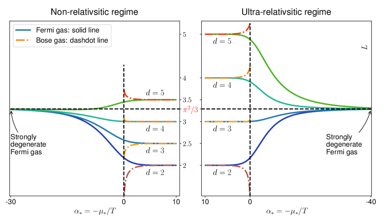
Figure 1: The Lorenz number

5 Concluding remarks

Guided by the viewpoint that observer is the key to bridge the gap between thermodynamics and relativity[39], the prior work presented a new collision model for relativistic Boltzmann equation and obtained a near equilibrium distribution function which is best used for studying transport phenomena in stationary spacetimes. The advantage of this distribution is illustrated by particle number transport where the effect of relativistic gravitational field is quite apparent. In this study, further examples are given to test the effectiveness of the distribution. The covariant transport equations for all the primary variables in the framework of relativistic kinetic theory are derived, surprisingly, the best interpretation of the results is rooted in Onsager theory for non-equilibrium processes. More concretely, both particle number flow and the internal energy flow are proportional to the thermodynamic forces, which, are identified as the generalized gradients of Massieu parameters. In this way, the kinetic coefficients are verified to obey the Onsager reciprocal relation which originally arose in non-relativistic statistical physics context.

The present work is built on top of relativistic kinetic theory and a specific, observer dependent collision model. The results are succinct and highly consistent with the conventional non-equilibrium thermodynamics. In addition, we proved the gravitational variant of the Wiedemann-Franz law and calculated the Lorenz number for neutral systems in gravitational field. Most notably, the Lorenz number for strongly degenerate Fermi gas takes a universal value $\pi^{2}/3$, which depends neither on the dimension and geometry of the spacetime, nor on the relativistic coldness. This result extends the Wiedemann-Franz law into the Wiedemann-Franz-Lorenz law [38].

It needs to be stressed that the present work considers only the transport equations for neutral relativistic systems subjecting to gravity. For astrophysical applications, the transport equations for charged relativistic systems subjecting to both gravitational and electromagnetic fields will be more appealing. Moreover, kinetic theory is not the only approach to non-equilibrium physics, some of the assumptions and models are well justified, but some approximations are applied for convenience and these must be checked against complementary statistical methods such as the stochastic processes, see, e.g. [40, 41, 42, 43, 44]. Nevertheless, we hope our preliminary treatment can be a stepping-stone in such areas.

Let us close this paper by adding the remark that, although we have chosen the stationary observer throughout this paper, the same construction should also work for other choices of observers. If other observers were considered, then the thermodynamic parameters for the system in detailed balance should get transformed in a way as discussed in [39]. Accordingly, the transport tensors should also acquire a transformation. Such transformations are not coordinate transformations but rather arise as the consequences of the choice of observers. This leaves us with an interesting question as to whether the form of the Onsager reciprocal relation and the Wiedemann-Franz law are observer independent. We hope to come back to this question in a later study.

Appendix A Corrections to the primary variables

We are free to choose any orthonormal basis $\{(e_{\hat{\alpha}})^{\mu}\}$, satisfying $\eta_{\hat{\alpha}\hat{\beta}}=g_{\mu\nu}(e_{\hat{\alpha}})^{\mu}(e_{\hat{\beta}})^{\nu}$, to in the tangent space at a given spacetime event, and in order to simplify the computation, it is convenient to fix the timelike leg such that $Z^{\mu}=(e_{\hat{0}})^{\mu}$. Then the projection tensor is simply given by

$$\Delta^{\mu\nu}=g^{\mu\nu}+Z^{\mu}Z^{\nu}=\delta^{\hat{a}\hat{b}}(e_{\hat{a}})^{\mu}(e_{\hat{b}})^{\nu}.$$

In this basis, the component of the momentum, $p^{\hat{\alpha}}=p^{\mu}(e^{\hat{\alpha}})_{\mu}$, can be parameterized by a real rapidity parameter $\vartheta$ and a spacelike unit vector $n^{\hat{a}}\in S^{d-1}$ as

$$p^{\hat{\alpha}} =m\left(\cosh\vartheta,~{}\sinh\vartheta\,n^{\hat{a}}\right).$$

The momentum space volume element then reduces to

$$\bm{\varpi} =\mathfrak{g}(m\sinh\vartheta)^{d-1}\mathrm{d}\vartheta\,\mathrm{d}\Omega_{d-1},$$

with $\mathrm{d}\Omega_{d-1}$ being the volume element of the $(d-1)$-dimensional unit sphere $S^{d-1}$. Therefore, the momentum space integral can be split into two parts, i.e. the integral over $\vartheta\in(0,\infty)$ and that over $S^{d-1}$. For the first part, we have introduced the function $J_{n,m}$ in eq.(9), and, for the second part, we note that

$$\int n^{\hat{a}}\mathrm{d}\Omega_{d-1}=0,\qquad\qquad\int n^{\hat{a}}n^{\hat{b}}\mathrm{d}\Omega_{d-1}=\frac{1}{d}\mathcal{A}_{d-1}\delta^{\hat{a}\hat{b}},$$

$$\int n^{\hat{a}}n^{\hat{b}}n^{\hat{c}}\mathrm{d}\Omega_{d-1}=0,\qquad\int n^{\hat{a}}n^{\hat{b}}n^{\hat{c}}n^{\hat{d}}\mathrm{d}\Omega_{d-1}=\frac{1}{d}\mathcal{A}_{d-1}\delta^{\hat{a}\hat{b}\hat{c}\hat{d}},$$

where $\mathcal{A}_{d-1}=\displaystyle\int\mathrm{d}\Omega_{d-1}$ is the area of a $(d-1)$-dimensional unit sphere, $\delta^{\hat{a}\hat{b}}$ is the Kronecker symbol and

$$\delta^{\hat{a}\hat{b}\hat{c}\hat{d}}\equiv\frac{1}{d+2}\left(\delta^{\hat{a}\hat{b}}\delta^{\hat{c}\hat{d}}+\delta^{\hat{a}\hat{c}}\delta^{\hat{b}\hat{d}}+\delta^{\hat{a}\hat{d}}\delta^{\hat{b}\hat{d}}\right),\qquad\delta^{\hat{a}\hat{b}\hat{c}\hat{d}}\,\delta_{\hat{c}\hat{d}}=\delta^{\hat{a}\hat{b}}.$$

The purpose of this appendix is to derive the expressions for $\delta N^{\mu}$, $\delta T^{\mu\nu}$ and $\delta S^{\mu}$ in terms of $(\alpha,\zeta,Z^{\mu})$, where, by definition,

$$N^{\mu} =\left[N^{(0)}\right]^{\mu}+\delta N^{\mu}=\int\bm{\varpi}p^{\mu}f^{(0)}+\int\bm{\varpi}p^{\mu}\delta f,$$

$$T^{\mu\nu} =\left[T^{(0)}\right]^{\mu\nu}+\delta T^{\mu\nu}=\int\bm{\varpi}p^{\mu}p^{\nu}f^{(0)}+\int\bm{\varpi}p^{\mu}p^{\nu}\delta f,$$

and

$$S^{\mu}=\left[S^{(0)}\right]^{\mu}+\delta S^{\mu},$$

with

$$S^{\mu}=-\int\bm{\varpi}p^{\mu}\left[f\log f-\varsigma^{-1}\left(1+\varsigma f\right)\log\left(1+\varsigma f\right)\right],$$

$$\left[S^{(0)}\right]^{\mu} =-\int\bm{\varpi}p^{\mu}\left[f^{(0)}\log f^{(0)}-\varsigma^{-1}\left(1+\varsigma f^{(0)}\right)\log\left(1+\varsigma f^{(0)}\right)\right],$$

and $f=f^{(0)}+\delta f$. Thinking of $\delta f$ as a small correction to $f^{(0)}$, one can easily get

$$\delta S^{\mu} =-\int\bm{\varpi}p^{\mu}\,\delta f\log\frac{f^{(0)}}{1+\varsigma f^{(0)}}=\alpha\,\delta N^{\mu}+\mathcal{B}_{\nu}\,\delta T^{\mu\nu}.$$

In order to outline the derivation of eq.(20), we need to recall that $\delta f$ is a combination of terms of orders $\mathcal{O}(\tau)$ and $\mathcal{O}(\tau^{2})$. Therefore, the correction terms to be evaluated should also be calculated up to the order $\mathcal{O}(\tau^{2})$. As intermediate results, let us list the following equations and identities,

$$\mathcal{D}_{\nu}f^{(0)}=\frac{1}{\beta}\frac{\partial f^{(0)}}{\partial\varepsilon}\left(\mathcal{D}_{\nu}\alpha+\varepsilon\,\mathcal{D}_{\nu}\beta\right),$$

$$\int\bm{\varpi}\,p^{\mu}f^{(0)}= \mathcal{\mathfrak{g}}m^{d}\mathcal{A}_{d-1}J_{d-1,1}\,Z^{\mu},$$

$$\int\bm{\varpi}\,p^{\mu}p^{\nu}f^{(0)}= \mathfrak{g}m^{d+1}\mathcal{A}_{d-1}\left(J_{d-1,2}\,Z^{\mu}Z^{\nu}+\frac{1}{d}J_{d+1,0}\,\Delta^{\mu\nu}\right),$$

$$\int\bm{\varpi}\,p^{\mu}p^{\nu}p^{\sigma}f^{(0)}= \mathfrak{g}m^{d+2}\mathcal{A}_{d-1}\left(J_{d-1,3}Z^{\mu}Z^{\nu}Z^{\sigma}+\frac{3}{d}J_{d+1,1}\Delta^{(\mu\nu}Z^{\sigma)}\right),$$

$$\Delta^{\alpha}{}_{\nu}\int\bm{\varpi}\,p^{\mu}p^{\nu}n^{\hat{a}}f^{(0)}= \mathfrak{g}m^{d+1}\frac{\mathcal{A}_{d-1}}{d}J_{d,1}Z^{\mu}(e^{\hat{a}})^{\alpha},$$

$$\Delta^{\alpha}{}_{\sigma}\int\bm{\varpi}\,p^{\mu}p^{\nu}p^{\sigma}n^{\hat{a}}f^{(0)}= \mathfrak{g}m^{d+2}\frac{\mathcal{A}_{d-1}}{d}\left[J_{d,2}\,Z^{\mu}Z^{\nu}(e^{\hat{a}})^{\alpha}+\frac{3}{d+2}J_{d+2,0}\,\Delta^{(\mu\nu}(e^{|\hat{a}|})^{\alpha)}\right].$$

The rest calculations are straightforward. At the order $\mathcal{O}(\tau)$, we have

$$\delta N^{\mu}\left[\mathcal{O}(\tau)\right]= -\frac{\tau}{m}\mathcal{D}_{\nu}\int\bm{\varpi}\,\frac{p^{\mu}p^{\nu}}{\cosh\vartheta}f^{(0)}$$

$$= -\tau\mathfrak{g}m^{d}\mathcal{A}_{d-1}\left(Z^{\mu}Z^{\nu}\mathcal{D}_{\nu}J_{d-1,1}+\frac{1}{d}\Delta^{\mu\nu}\mathcal{D}_{\nu}J_{d+1,-1}\right),$$

$$\delta T^{\mu\nu}\left[\mathcal{O}(\tau)\right]= -\frac{\tau}{m}\mathcal{D}_{\sigma}\int\bm{\varpi}\,\frac{p^{\mu}p^{\nu}p^{\sigma}}{\cosh\vartheta}f^{(0)}$$

$$= -\tau\mathfrak{g}m^{d+1}\mathcal{A}_{d-1}\left(Z^{\mu}Z^{\nu}Z^{\sigma}\mathcal{D}_{\sigma}J_{d-1,2}+\frac{3}{d}\Delta^{(\mu\nu}Z^{\sigma)}\mathcal{D}_{\sigma}J_{d+1,0}\right),$$

where

$$\mathcal{D}_{\sigma}J_{m,n}=\frac{\partial J_{m,n}}{\partial\alpha}\mathcal{D}_{\nu}\alpha+\frac{\partial J_{m,n}}{\partial\zeta}\mathcal{D}_{\nu}\zeta=-\mathcal{J}_{m,n}\mathcal{D}_{\sigma}\alpha-\mathcal{J}_{m,n+1}\mathcal{D}_{\sigma}\zeta.$$

Next, at the order $\mathcal{O}(\tau^{2})$, we have

$$\delta N^{\mu}\left[\mathcal{O}(\tau^{2})\right]= -\frac{\tau^{2}}{m}\Delta^{\alpha}{}_{\sigma}\nabla_{[\alpha}Z_{\beta]}\Delta^{\beta\nu}\mathcal{D}_{\nu}\int\bm{\varpi}\,\frac{p^{\mu}p^{\sigma}}{\cosh\vartheta}f^{(0)}$$

$$-\frac{\tau^{2}}{m}\Delta^{\alpha}{}_{\sigma}\nabla_{[\alpha}(e_{|\hat{a}|})_{\beta]}\Delta^{\beta\nu}\mathcal{D}_{\nu}\int\bm{\varpi}\,\frac{p^{\mu}p^{\sigma}n^{\hat{a}}\sinh\vartheta}{\cosh^{2}\vartheta}f^{(0)}$$

$$= -\tau^{2}\mathfrak{g}m^{d}\frac{\mathcal{A}_{d-1}}{d}\left(B^{\mu\nu}+Z^{\mu}\mathfrak{B}^{\nu}\right)\mathcal{D}_{\nu}J_{d+1,-1},$$

$$\delta T^{\mu\nu}\left[\mathcal{O}(\tau^{2})\right]= -\frac{\tau^{2}}{m}\Delta^{\alpha}{}_{\rho}\nabla_{[\alpha}Z_{\beta]}\Delta^{\beta\sigma}\mathcal{D}_{\sigma}\int\bm{\varpi}\,\frac{p^{\mu}p^{\nu}p^{\rho}}{\cosh\vartheta}f^{(0)}$$

$$-\frac{\tau^{2}}{m}\Delta^{\alpha}{}_{\rho}\nabla_{[\alpha}(e_{|\hat{a}|})_{\beta]}\Delta^{\beta\sigma}\mathcal{D}_{\sigma}\int\bm{\varpi}\,\frac{p^{\mu}p^{\nu}p^{\rho}n^{\hat{a}}\sinh\vartheta}{\cosh^{2}\vartheta}f^{(0)}$$

$$= -\tau^{2}\mathfrak{g}m^{d+1}\frac{\mathcal{A}_{d-1}}{d}\left(Z^{(\mu}B^{\nu)\sigma}+Z^{\mu}Z^{\nu}\mathfrak{B}^{\sigma}\right)\mathcal{D}_{\sigma}J_{d+1,0}$$

$$-\tau^{2}\mathfrak{g}m^{d+1}\frac{\mathcal{A}_{d-1}}{d(d+2)}\left(\Delta^{\mu\nu}\mathfrak{B}^{\sigma}+\mathfrak{B}^{\mu\nu\sigma}+\mathfrak{B}^{\nu\mu\sigma}\right)\mathcal{D}_{\sigma}J_{d+3,-2},$$

where $B_{\mu\nu}$ and $\mathfrak{B}^{\sigma}{}_{\mu\nu}$ are defined as in eqs.(18) and (19). Finally, summing up contributions of orders $\mathcal{O}(\tau)$ and $\mathcal{O}(\tau^{2})$ together and rearranging terms, we obtain the results listed in eq.(20).

Appendix B Lorenz number in the cases $\zeta\gg 1$ and $\zeta\ll 1$

The aim of this section is to simplify Lorenz number (35) in the limits $\zeta\gg 1$ and $\zeta\ll 1$. Therefore, we take $n=d+1$ and $m=-1,0,1$.

In terms of the variable $u=\zeta(\cosh\vartheta-1)$, we have

$$\cosh\vartheta=\dfrac{u}{\zeta}+1,\quad\sinh\vartheta=\sqrt{\frac{u^{2}}{\zeta^{2}}+2\frac{u}{\zeta}},\quad\mathrm{d}\vartheta=\frac{\mathrm{d}u}{\zeta\sinh\vartheta},$$

and the integral $J_{n,m}$ becomes

$$J_{n,m}=\frac{1}{\zeta}\int_{0}^{\infty}\frac{\left(\frac{u^{2}}{\zeta^{2}}+2\frac{u}{\zeta}\right)^{{n-1}\over{2}}\left(\frac{u}{\zeta}+1\right)^{m}}{\mathrm{e}^{\alpha_{*}+u}-\varsigma}\mathrm{d}u.$$

In the non-relativistic limit $\zeta\gg 1$, $J_{n,m}$ is approximately

$$J_{n,m} \approx\frac{1}{2}\left(\frac{2}{\zeta}\right)^{{n+1}\over{2}}\int_{0}^{\infty}\frac{u^{{n-1}\over{2}}\left(\frac{u}{\zeta}+1\right)^{m}\mathrm{d}\vartheta}{\mathrm{e}^{\alpha_{*}+u}-\varsigma}$$

$$\approx\frac{1}{2}\left(\frac{2}{\zeta}\right)^{{n+1}\over{2}}\bigg{[}\int_{0}^{\infty}\frac{u^{{n-1}\over{2}}\mathrm{d}\vartheta}{\mathrm{e}^{\alpha_{*}+u}-\varsigma}+\frac{m}{\zeta}\int_{0}^{\infty}\frac{u^{{n+1}\over{2}}\mathrm{d}\vartheta}{\mathrm{e}^{\alpha_{*}+u}-\varsigma}+\frac{m(m-1)}{2\zeta^{2}}\int_{0}^{\infty}\frac{u^{{n+3}\over{2}}\mathrm{d}\vartheta}{\mathrm{e}^{\alpha_{*}+u}-\varsigma}\bigg{]}$$

$$\approx\frac{1}{2}\left(\frac{2}{\zeta}\right)^{{n+1}\over{2}}\varsigma\bigg{[}\Gamma\left(\frac{n+1}{2}\right)\mathrm{Li}_{\frac{n+1}{2}}\left(\varsigma\mathrm{e}^{-\alpha_{*}}\right)$$

$$~{}~{}~{}~{}+\frac{m}{\zeta}\Gamma\left(\frac{n+3}{2}\right)\mathrm{Li}_{\frac{n+3}{2}}\left(\varsigma\mathrm{e}^{-\alpha_{*}}\right)+\frac{m(m-1)}{2\zeta^{2}}\Gamma\left(\frac{n+5}{2}\right)\mathrm{Li}_{\frac{n+5}{2}}\left(\varsigma\mathrm{e}^{-\alpha_{*}}\right)\bigg{]},$$

therefore, $\mathcal{J}_{n,m}=-\dfrac{\partial}{\partial\alpha}J_{n,m}=-\dfrac{\partial}{\partial\alpha_{*}}J_{n,m}$ becomes

$$\mathcal{J}_{n,m}\approx\, \frac{1}{2}\left(\frac{2}{\zeta}\right)^{\frac{n+1}{2}}\varsigma\bigg{[}\Gamma\left(\frac{n+1}{2}\right)\mathrm{Li}_{\frac{n-1}{2}}\left(\varsigma\mathrm{e}^{-\alpha_{*}}\right)$$

$$+\frac{m}{\zeta}\Gamma\left(\frac{n+3}{2}\right)\mathrm{Li}_{\frac{n+1}{2}}\left(\varsigma\mathrm{e}^{-\alpha_{*}}\right)+\frac{m(m-1)}{2\zeta^{2}}\Gamma\left(\frac{n+5}{2}\right)\mathrm{Li}_{\frac{n+3}{2}}\left(\varsigma\mathrm{e}^{-\alpha_{*}}\right)\bigg{]}.$$

The Lorenz number is then simplified to be

$$L\approx\frac{d+2}{2}\left[\frac{d+4}{2}\frac{\mathrm{Li}_{\frac{d+4}{2}}\left(\varsigma\mathrm{e}^{-\alpha_{*}}\right)}{\mathrm{Li}_{\frac{d}{2}}\left(\varsigma\mathrm{e}^{-\alpha_{*}}\right)}-\frac{d+2}{2}\frac{\mathrm{Li}_{\frac{d+2}{2}}\left(\varsigma\mathrm{e}^{-\alpha_{*}}\right)^{2}}{\mathrm{Li}_{\frac{d}{2}}\left(\varsigma\mathrm{e}^{-\alpha_{*}}\right)^{2}}\right].$$ (40)

On the other hand, in the ultra-relativistic limit $\zeta\ll 1$,

$$J_{n,m} \approx\left(\frac{1}{\zeta}\right)^{m+n}\int_{0}^{\infty}\frac{u^{m+n-1}\mathrm{d}\vartheta}{\mathrm{e}^{\alpha_{*}+u}-1}=\left(\frac{1}{\zeta}\right)^{m+n}\Gamma(m+n)\,\mathrm{Li}_{m+n}(\mathrm{e}^{-\alpha_{*}}).$$

In this case,

$$\mathcal{J}_{n,m}=-\frac{\partial}{\partial\alpha}J_{n,m}\approx\left(\frac{1}{\zeta}\right)^{m+n}\Gamma(m+n)\,\mathrm{Li}_{m+n-1}(\mathrm{e}^{-\alpha_{*}}),$$

and correspondingly,

$$L\approx d\left[(d+1)\frac{\mathrm{Li}_{d+1}\left(\varsigma\mathrm{e}^{-\alpha_{*}}\right)}{\mathrm{Li}_{d-1}\left(\varsigma\mathrm{e}^{-\alpha_{*}}\right)}-d\frac{\mathrm{Li}_{d}\left(\varsigma\mathrm{e}^{-\alpha_{*}}\right)^{2}}{\mathrm{Li}_{d-1}\left(\varsigma\mathrm{e}^{-\alpha_{*}}\right)^{2}}\right].$$ (41)

Finally, eqs.(40) and (41) can be summarized in the unified form (36).

Appendix C Universal $L$ for strongly degenerate Fermi gas

Here we outline the procedure for obtaining the universal result for the Lorenz number of strongly degenerate Fermi gas. We first introduce the variables $u=\zeta(\cosh\vartheta-1)$ and $u_{0}=-\alpha_{*}$. Then we can write

$$J_{n,m} =\int_{0}^{\infty}\frac{\sinh^{n}\vartheta\cosh^{m}\vartheta\mathrm{d}\vartheta}{\mathrm{e}^{\alpha+\zeta\cosh\vartheta}+1}=\int_{0}^{\infty}\frac{\mathrm{d}\varphi(u)}{\mathrm{e}^{u-u_{0}}+1},$$

where

$$\varphi(u)=\frac{1}{n+1}\sinh^{n+1}\left[\operatorname{arcosh}\left(\frac{u+\zeta}{\zeta}\right)\right]\mathcal{F}_{\frac{1-m}{2},\frac{n+1}{2}}\left[\operatorname{arcosh}\left(\frac{u+\zeta}{\zeta}\right)\right],$$

and $\mathcal{F}_{a,b}(\vartheta)$ is the following Gaussian hypergeometric function

$$\mathcal{F}_{a,b}(\vartheta)\equiv\,_{2}F_{1}\left(a,b;b+1;-\sinh^{2}\vartheta\right).$$

According to Sommerfeld’s lemma, the following integral can be approximately expressed as

$$\int_{0}^{\infty}\frac{\mathrm{d}\varphi(u)}{\mathrm{e}^{u-u_{0}}+1}\approx\varphi(u_{0})+\frac{\pi^{2}}{6}\varphi^{\prime\prime}(u_{0})+\cdots,$$

provided $\varphi(0)=0$, $\displaystyle\lim_{u\to\infty}\frac{\varphi(u)}{\mathrm{e}^{u-u_{0}}+1}=0$ and $u_{0}\gg 1$. Therefore, we have

$$J_{n,m}\approx\varphi(-\alpha_{*})+\frac{\pi^{2}}{6}\varphi^{\prime\prime}(-\alpha_{*}),$$

and further,

$$\mathcal{J}_{n,m}=-\frac{\partial}{\partial\alpha}J_{n,m}\approx\varphi^{\prime}(-\alpha_{*})+\frac{\pi^{2}}{6}\varphi^{\prime\prime\prime}(-\alpha_{*}),$$

where

$$\varphi^{\prime}(-\alpha_{*}) =\frac{1}{\zeta}\left(-\frac{\alpha}{\zeta}\right)^{m}\sinh^{n-1}\left[\operatorname{arcosh}\left(-\frac{\alpha}{\zeta}\right)\right],$$

$$\varphi^{\prime\prime\prime}(-\alpha_{*}) =\frac{\pi^{2}}{6}\frac{1}{\zeta^{3}}\bigg{\{}(m+n-1)(m+n-2)\left(-\frac{\alpha}{\zeta}\right)^{m+2}+m(m-1)\left(-\frac{\alpha}{\zeta}\right)^{m-2}$$

$$~{}~{}~{}~{}~{}~{}~{}~{}~{}~{}~{}~{}~{}-\left[2m(m+n-2)+n-1\right]\left(-\frac{\alpha}{\zeta}\right)^{m}\bigg{\}}\sinh^{n-5}\left[\operatorname{arcosh}\left(-\frac{\alpha}{\zeta}\right)\right].$$

Inserting the above approximate result for $\mathcal{J}_{n,m}$ into eq.(35) and making some further simplifications, we get the desired result (39).

Data Availability Statement

This work is purely theoretical and contains only analytic analysis. Hence there is no associated numeric data.

Declaration of competing interest

The authors declare no competing interest.