Multimodal Learning Without Labeled Multimodal Data:
Guarantees and Applications

Abstract

In many machine learning systems that jointly learn from multiple modalities, a core research question is to understand the nature of multimodal interactions: the emergence of new task-relevant information during learning from both modalities that was not present in either alone. We study this challenge of interaction quantification in a semi-supervised setting with only labeled unimodal data and naturally co-occurring multimodal data (e.g., unlabeled images and captions, video and corresponding audio) but when labeling them is time-consuming. Using a precise information-theoretic definition of interactions, our key contributions are the derivations of lower and upper bounds to quantify the amount of multimodal interactions in this semi-supervised setting. We propose two lower bounds based on the amount of shared information between modalities and the disagreement between separately trained unimodal classifiers, and derive an upper bound through connections to approximate algorithms for min-entropy couplings. We validate these estimated bounds and show how they accurately track true interactions. Finally, two semi-supervised multimodal applications are explored based on these theoretical results: (1) analyzing the relationship between multimodal performance and estimated interactions, and (2) self-supervised learning that embraces disagreement between modalities beyond agreement as is typically done.

1 Introduction

A core research question in multimodal learning is to understand the nature of multimodal interactions across modalities in the context of a task: the emergence of new task-relevant information during learning from both modalities that was not present in either modality alone [6, 65]. In settings where labeled multimodal data is abundant, the study of multimodal interactions has inspired advances in theoretical analysis [1, 43, 66, 84, 94] and representation learning [51, 76, 91, 104] in language and vision [2], multimedia [9], healthcare [53], and robotics [57]. In this paper, we study the problem of interaction quantification in a setting where there is only unlabeled multimodal data $\mathcal{D}_{M}=\{(x_{1},x_{2})\}$ but some labeled unimodal data $\mathcal{D}_{i}=\{(x_{i},y)\}$ collected separately for each modality. This multimodal semi-supervised paradigm is reminiscent of many real-world settings with the emergence of separate unimodal datasets like large-scale visual recognition [23] and text classification [96], as well as the collection of data in multimodal settings (e.g., unlabeled images and captions or video and audio [63, 87, 76, 107]) but when labeling them is time-consuming [47, 48].

Using a precise information-theoretic definition of interactions [10, 98], our key contributions are the derivations of lower and upper bounds to quantify the amount of multimodal interactions in this semi-supervised setting with only $\mathcal{D}_{i}$ and $\mathcal{D}_{M}$. We propose two lower bounds for interaction quantification: our first lower bound relates multimodal interactions with the amount of shared information between modalities, and our second lower bound introduces the concept of modality disagreement which quantifies the differences of classifiers trained separately on each modality. Finally, we propose an upper bound through connections to approximate algorithms for min-entropy couplings [16]. To validate our derivations, we experiment on large-scale synthetic and real-world datasets with varying amounts of interactions. In addition, these theoretical results naturally yield new algorithms for two applications involving semi-supervised multimodal data:

1. We first analyze the relationship between interaction estimates and downstream task performance when optimal multimodal classifiers are learned access to multimodal data. This analysis can help develop new guidelines for deciding when to collect and fuse labeled multimodal data.

2. As the result of our analysis, we further design a new family of self-supervised learning objectives that capture disagreement on unlabeled multimodal data, and show that this learns interactions beyond agreement conventionally used in the literature [76, 81, 107]. Our experiments show strong results on four datasets: relating cartoon images and captions [44], predicting expressions of humor and sarcasm from videos [14, 40], and reasoning about multi-party social interactions [105].

More importantly, these results shed light on the intriguing connections between disagreement, interactions, and performance. Our code is available at https://github.com/pliang279/PID.

2 Preliminaries

2.1 Definitions and setup

Let $\mathcal{X}_{i}$ and $\mathcal{Y}$ be finite sample spaces for features and labels. Define $\Delta$ to be the set of joint distributions over $(\mathcal{X}_{1},\mathcal{X}_{2},\mathcal{Y})$. We are concerned with features $X_{1},X_{2}$ (with support $\mathcal{X}_{i}$) and labels $Y$ (with support $\mathcal{Y}$) drawn from some distribution $p\in\Delta$. We denote the probability mass function by $p(x_{1},x_{2},y)$, where omitted parameters imply marginalization. In many real-world applications [63, 76, 81, 102, 107], we only have partial datasets from $p$ rather than the full distribution:

• Labeled unimodal data $\mathcal{D}_{1}=\{(x_{1},y):\mathcal{X}_{1}\times\mathcal{Y}\}$, $\mathcal{D}_{2}=\{(x_{2},y):\mathcal{X}_{2}\times\mathcal{Y}\}$.

• Unlabeled multimodal data $\mathcal{D}_{M}=\{(x_{1},x_{2}):\mathcal{X}_{1}\times\mathcal{X}_{2}\}$.

$\mathcal{D}_{1}$, $\mathcal{D}_{2}$ and $\mathcal{D}_{M}$ follow the pairwise marginals $p(x_{1},y)$, $p(x_{2},y)$ and $p(x_{1},x_{2})$. We define $\Delta_{p_{1,2}}=\{q\in\Delta:q(x_{i},y)=p(x_{i},y)\ \forall y\in\mathcal{Y},x_{i}\in\mathcal{X}_{i},i\in[2]\}$ as the set of joint distributions which agree with the labeled unimodal data $\mathcal{D}_{1}$ and $\mathcal{D}_{2}$, and $\Delta_{p_{1,2,12}}=\{r\in\Delta:r(x_{1},x_{2})=p(x_{1},x_{2}),r(x_{i},y)=p(x_{i},y)\}$ as the set of joint distributions which agree with all $\mathcal{D}_{1},\mathcal{D}_{2}$ and $\mathcal{D}_{M}$.

Despite partial observability, we often still want to understand the degree to which two modalities can interact to contribute new information not present in either modality alone, in order to inform our decisions on multimodal data collection and modeling [51, 60, 66, 104]. We now cover background towards a formal information-theoretic definition of interactions and their approximation.

2.2 Information theory, partial information decomposition, and synergy

Information theory formalizes the amount of information that a variable ($X_{1}$) provides about another ($X_{2}$), and is quantified by Shannon’s mutual information (MI) and conditional MI [80]:

$$I(X_{1};X_{2})=\int p(x_{1},x_{2})\log\frac{p(x_{1},x_{2})}{p(x_{1})p(x_{2})}d\bm{x},\quad I(X_{1};X_{2}|Y)=\int p(x_{1},x_{2}|y)\log\frac{p(x_{1},x_{2}|y)}{p(x_{1}|y)p(x_{2}|y)}d\bm{x}dy.$$

The MI of two random variables $X_{1}$ and $X_{2}$ measures the amount of information (in bits) obtained about $X_{1}$ by observing $X_{2}$, and by extension, conditional MI is the expected value of MI given the value of a third (e.g., $Y$). However, the extension of information theory to three or more variables to describe the synergy between two modalities for a task remains an open challenge. Among many proposed frameworks, Partial information decomposition (PID) [98] posits a decomposition of the total information $2$ variables $X_{1},X_{2}$ provide about a task $Y$ into 4 quantities: $I_{p}(\{X_{1},X_{2}\};Y)=R+U_{1}+U_{2}+S$ where $I_{p}(\{X_{1},X_{2}\};Y)$ is the MI between the joint random variable $(X_{1},X_{2})$ and $Y$, redundancy $R$ describes task-relevant information shared between $X_{1}$ and $X_{2}$, uniqueness $U_{1}$ and $U_{2}$ studies the task-relevant information present in only $X_{1}$ or $X_{2}$ respectively, and synergy $S$ investigates the emergence of new information only when both $X_{1}$ and $X_{2}$ are present [10, 38]:

Definition 1.

(Multimodal interactions) Given $X_{1}$, $X_{2}$, and a target $Y$, we define their redundant ($R$), unique ($U_{1}$ and $U_{2}$), and synergistic ($S$) interactions as:

$$R =\max_{q\in\Delta_{p_{1,2}}}I_{q}(X_{1};X_{2};Y),\quad U_{1}=\min_{q\in\Delta_{p_{1,2}}}I_{q}(X_{1};Y|X_{2}),\quad U_{2}=\min_{q\in\Delta_{p_{1,2}}}I_{q}(X_{2};Y|X_{1}),$$ (1)

$$S =I_{p}(\{X_{1},X_{2}\};Y)-\min_{q\in\Delta_{p_{1,2}}}I_{q}(\{X_{1},X_{2}\};Y),$$ (2)

where the notation $I_{p}(\cdot)$ and $I_{q}(\cdot)$ disambiguates mutual information (MI) under $p$ and $q$ respectively.

$I(X_{1};X_{2};Y)=I(X_{1};X_{2})-I(X_{1};X_{2}|Y)$ is a multivariate extension of information theory [8, 70]. Most importantly, $R$, $U_{1}$, and $U_{2}$ can be computed exactly using convex programming over distributions $q\in\Delta_{p_{1,2}}$ with access only to the marginals $p(x_{1},y)$ and $p(x_{2},y)$ by solving an equivalent max-entropy optimization problem $q^{*}=\operatorname*{arg\,max}_{q\in\Delta_{p_{1,2}}}H_{q}(Y|X_{1},X_{2})$ [10, 66]. This is a convex optimization problem with linear marginal-matching constraints (see Appendix A.2). This gives us an elegant interpretation that we need only labeled unimodal data in each feature from $\mathcal{D}_{1}$ and $\mathcal{D}_{2}$ to estimate redundant and unique interactions.

3 Estimating Synergy Without Multimodal Data

Unfortunately, $S$ is impossible to compute via equation (2) when we do not have access to the full joint distribution $p$, since the first term $I_{p}(X_{1},X_{2};Y)$ is unknown. Instead, we will aim to provide lower and upper bounds in the form $\underline{S}\leq S\leq\overline{S}$ which depend only on $\mathcal{D}_{1}$, $\mathcal{D}_{2}$, and $\mathcal{D}_{M}$.

3.1 Lower bounds on synergy

Our first insight is that while labeled multimodal data is unavailable, the output of unimodal classifiers may be compared against each other. Let $\delta_{\mathcal{Y}}=\{r\in\mathbb{R}_{+}^{|\mathcal{Y}|}\ |\ ||r||_{1}=1\}$ be the probability simplex over labels $\mathcal{Y}$. Consider the set of unimodal classifiers $\mathcal{F}_{i}\ni f_{i}:\mathcal{X}_{i}\rightarrow\delta_{\mathcal{Y}}$ and multimodal classifiers $\mathcal{F}_{M}\ni f_{M}:\mathcal{X}_{1}\times\mathcal{X}_{2}\rightarrow\delta_{\mathcal{Y}}$. The crux of our method is to establish a connection between modality disagreement and a lower bound on synergy.

Definition 2.

(Modality disagreement) Given $X_{1}$, $X_{2}$, and a target $Y$, as well as unimodal classifiers $f_{1}$ and $f_{2}$, we define modality disagreement as $\alpha(f_{1},f_{2})=\mathbb{E}_{p(x_{1},x_{2})}[d(f_{1},f_{2})]$ where $d:\mathcal{Y}\times\mathcal{Y}\rightarrow\mathbb{R}^{\geq 0}$ is a distance function in label space scoring the disagreement of $f_{1}$ and $f_{2}$’s predictions.

Quantifying modality disagreement gives rise to two types of synergy as illustrated in Figure 1: agreement synergy and disagreement synergy. As their names suggest, agreement synergy happens when two modalities agree in predicting the label and synergy arises within this agreeing information. On the other hand, disagreement synergy happens when two modalities disagree in predicting the label, and synergy arises due to disagreeing information.

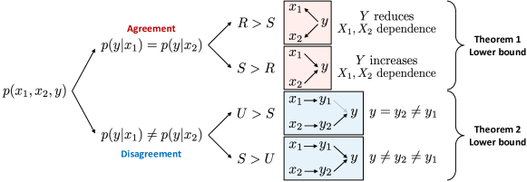
Figure 1: We estimate two types of synergy: (1) agreement synergy that arises as a result of $Y$ increasing the agreeing shared information between $X_{1}$ and $X_{2}$ (reminiscent of common cause structures as opposed to redundancy in common effect), and (2) disagreement synergy that emerges due to the disagreement between unimodal predictors resulting in a new prediction $y\neq y_{1}\neq y_{2}$ (rather than uniqueness where $y=y_{2}\neq y_{1}$).

Agreement synergy

We first consider the case when two modalities contain shared information that leads to agreement in predicting the outcome. In studying these situations, a driving force for estimating $S$ is the amount of shared information $I(X_{1};X_{2})$ between modalities, with the intuition that more shared information naturally leads to redundancy which gives less opportunity for new synergistic interactions. Mathematically, we formalize this by relating $S$ to $R$ [98],

$$S=R-I_{p}(X_{1};X_{2};Y)=R-I_{p}(X_{1};X_{2})+I_{p}(X_{1};X_{2}|Y).$$ (3)

implying that synergy exists when there is high redundancy and low (or even negative) three-way MI $I_{p}(X_{1};X_{2};Y)$ [7, 35]. By comparing the difference in $X_{1},X_{2}$ dependence with and without the task (i.e., $I_{p}(X_{1};X_{2})$ vs $I_{p}(X_{1};X_{2}|Y)$), $2$ cases naturally emerge (see top half of Figure 1):

1. $\mathbf{S>R}$: When both modalities do not share a lot of information as measured by low $I(X_{1};X_{2})$, but conditioning on $Y$ increases their dependence: $I(X_{1};X_{2}|Y)>I(X_{1};X_{2})$, then there is synergy between modalities when combining them for task $Y$. This setting is reminiscent of common cause structures. Examples of these distributions in the real world are multimodal question answering, where the image and question are less dependent (some questions like ‘what is the color of the car’ or ‘how many people are there’ can be asked for many images), but the answer (e.g., ‘blue car’) connects the two modalities, resulting in dependence given the label. As expected, $S=4.92,R=0.79$ for the VQA 2.0 dataset [37].

2. $\mathbf{R>S}$: Both modalities share a lot of information but conditioning on $Y$ reduces their dependence: $I(X_{1};X_{2})>I(X_{1};X_{2}|Y)$, which results in more redundant than synergistic information. This setting is reminiscent of common effect structures. A real-world example is in detecting sentiment from multimodal videos, where text and video are highly dependent since they are emitted by the same speaker, but the sentiment label explains away some of the dependencies between both modalities. Indeed, for multimodal sentiment analysis from text, video, and audio of monologue videos on MOSEI [59, 106], $R=0.26$ and $S=0.04$.

However, $I_{p}(X_{1};X_{2}|Y)$ cannot be computed without access to the full distribution $p$. In Theorem 1, we obtain a lower bound on $I_{p}(X_{1};X_{2}|Y)$, resulting in a lower bound $\underline{S}_{\textrm{agree}}$ for synergy.

Theorem 1.

(Lower-bound on synergy via redundancy) We can relate $S$ to $R$ as follows

$$\underline{S}_{\textrm{agree}}=R-I_{p}(X_{1};X_{2})+\min_{r\in\Delta_{p_{1,2,12}}}I_{r}(X_{1};X_{2}|Y)\leq S$$ (4)

We include the full proof in Appendix A.3, but note that $\min_{r\in\Delta_{p_{1,2,12}}}I_{r}(X_{1};X_{2}|Y)$ is equivalent to a max-entropy optimization problem solvable using convex programming. This implies that $\underline{S}_{\textrm{agree}}$ can be computed efficiently using only unimodal data $\mathcal{D}_{i}$ and unlabeled multimodal data $\mathcal{D}_{M}$.

Disagreement synergy

We now consider settings where two modalities disagree in predicting the outcome: suppose $y_{1}=\operatorname*{arg\,max}_{y}p(y|x_{1})$ is the most likely prediction from the first modality, $y_{2}=\operatorname*{arg\,max}_{y}p(y|x_{2})$ for the second modality, and $y=\operatorname*{arg\,max}_{y}p(y|x_{1},x_{2})$ the true multimodal prediction. During disagreement, there are again $2$ cases (see bottom half of Figure 1):

1. $\mathbf{U>S}$: Multimodal prediction $y=\operatorname*{arg\,max}_{y}p(y|x_{1},x_{2})$ is the same as one of the unimodal predictions (e.g., $y=y_{2}$), in which case unique information in modality $2$ leads to the outcome. A real-world dataset that we categorize in this case is MIMIC involving mortality and disease prediction from tabular patient data and time-series medical sensors [53] which primarily shows unique information in the tabular modality. The disagreement on MIMIC is high $\alpha=0.13$, but since disagreement is due to a lot of unique information, there is less synergy $S=0.01$.

2. $\mathbf{S>U}$: Multimodal prediction $y$ is different from both $y_{1}$ and $y_{2}$, then both modalities interact synergistically to give rise to a final outcome different from both disagreeing unimodal predictions. This type of joint distribution is indicative of real-world examples such as predicting sarcasm from language and speech - the presence of sarcasm is typically detected due to a contradiction between what is expressed in language and speech, as we observe from the experiments on MUStARD [14] where $S=0.44$ and $\alpha=0.12$ are both relatively large.

We formalize these intuitions via Theorem 2, yielding a lower bound $\underline{S}_{\textrm{disagree}}$ based on disagreement minus the maximum unique information in both modalities:

Theorem 2.

(Lower-bound on synergy via disagreement, informal) We can relate synergy $S$ and uniqueness $U$ to modality disagreement $\alpha(f_{1},f_{2})$ of optimal unimodal classifiers $f_{1},f_{2}$ as follows:

$$\underline{S}_{\textrm{disagree}}=\alpha(f_{1},f_{2})\cdot c-\max(U_{1},U_{2})\leq S$$ (5)

for some constant $c$ depending on the label dimension $|\mathcal{Y}|$ and choice of label distance function $d$.

Theorem 2 implies that if there is substantial disagreement $\alpha(f_{1},f_{2})$ between unimodal classifiers, it must be due to the presence of unique or synergistic information. If uniqueness is small, then disagreement must be accounted for by synergy, thereby yielding a lower bound $\underline{S}_{\textrm{disagree}}$. Note that the notion of optimality in unimodal classifiers is important: poorly-trained unimodal classifiers could show high disagreement but would be uninformative about true interactions. We include the formal version of the theorem based on Bayes’ optimality and a full proof in Appendix A.4.

Hence, agreement and disagreement synergy yield separate lower bounds $\underline{S}_{\textrm{agree}}$ and $\underline{S}_{\textrm{disagree}}$. Note that these bounds always hold, so we could take $\underline{S}=\max\{\underline{S}_{\textrm{agree}},\underline{S}_{\textrm{disagree}}\}$.

3.2 Upper bound on synergy

While the lower bounds tell us the least amount of synergy possible in a distribution, we also want to obtain an upper bound on the possible synergy, which together with the above lower bounds sandwich $S$. By definition, $S=I_{p}(\{X_{1},X_{2}\};Y)-\max_{q\in\Delta_{p_{1,2}}}I_{q}(\{X_{1},X_{2}\};Y)$. Thus, upper bounding synergy is the same as maximizing the MI $I_{p}(X_{1},X_{2};Y)$, which can be rewritten as

$$\max_{r\in\Delta_{p_{1,2,12}}}I_{r}(\{X_{1},X_{2}\};Y) =\max_{r\in\Delta_{p_{1,2,12}}}\left\{H_{r}(X_{1},X_{2})+H_{r}(Y)-H_{r}(X_{1},X_{2},Y)\right\}$$ (6)

$$=H_{p}(X_{1},X_{2})+H_{p}(Y)-\min_{r\in\Delta_{p_{1,2,12}}}H_{r}(X_{1},X_{2},Y),$$ (7)

where the second line follows from the definition of $\Delta_{p_{1,2,12}}$. Since the first two terms are constant, an upper bound on $S$ requires us to look amongst all multimodal distributions $r\in\Delta$ which match the unimodal $\mathcal{D}_{i}$ and unlabeled multimodal data $\mathcal{D}_{M}$, and find the one with minimum entropy.

Theorem 3.

Solving $r^{*}=\operatorname*{arg\,min}_{r\in\Delta_{p_{1,2,12}}}H_{r}(X_{1},X_{2},Y)$ is NP-hard, even for a fixed $|\mathcal{Y}|\geq 4$.

Theorem 3 suggests we cannot tractably find a joint distribution which tightly upper bounds synergy when the feature spaces are large. Thus, our proposed upper bound $\overline{S}$ is based on a lower bound on $\min_{r\in\Delta_{p_{1,2,12}}}H_{r}(X_{1},X_{2},Y)$, which yields

Theorem 4.

(Upper-bound on synergy)

$$S\leq H_{p}(X_{1},X_{2})+H_{p}(Y)-\min_{r\in\Delta_{p_{12,y}}}H_{r}(X_{1},X_{2},Y)-\max_{q\in\Delta_{p_{1,2}}}I_{q}(\{X_{1},X_{2}\};Y)=\overline{S}$$ (8)

where $\Delta_{p_{12,y}}=\{r\in\Delta:r(x_{1},x_{2})=p(x_{1},x_{2}),r(y)=p(y)\}$. The second optimization problem is solved with convex optimization. The first is the classic min-entropy coupling over $(X_{1},X_{2})$ and $Y$, which is still NP-hard but admits good approximations [16, 17, 55, 78, 19, 20]. Proofs of Theorem 3, 4, and approximations for min-entropy couplings are deferred to Appendix A.5 and A.6.

4 Experiments

We design comprehensive experiments to validate these estimated bounds and show new relationships between disagreement, multimodal interactions, and performance, before describing two applications in (1) estimating optimal multimodal performance without multimodal data to prioritize the collection and fusion data sources, and (2) a new disagreement-based self-supervised learning method.

4.1 Verifying predicted guarantees and analysis of multimodal distributions

Synthetic bitwise datasets: We enumerate joint distributions over $\mathcal{X}_{1},\mathcal{X}_{2},\mathcal{Y}\in\{0,1\}$ by sampling $100,000$ vectors in the 8-dimensional probability simplex and assigning them to each $p(x_{1},x_{2},y)$. Using these distributions, we estimate $\hat{p}(y|x_{1})$ and $\hat{p}(y|x_{2})$ to compute disagreement and the marginals $\hat{p}(x_{1},y)$, $\hat{p}(x_{2},y)$, and $\hat{p}(x_{1},x_{2})$ to estimate the lower and upper bounds.

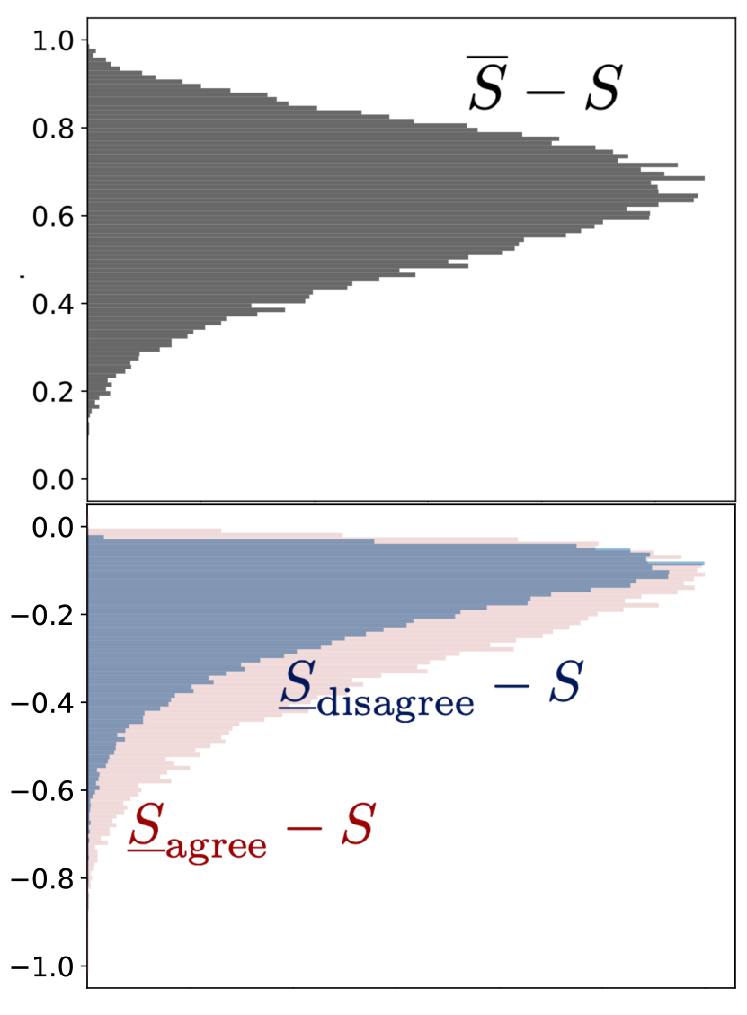
Figure 2: Our two lower bounds $\underline{S}_{\textrm{agree}}$ and $\underline{S}_{\textrm{disagree}}$ track actual synergy $S$ from below, and the upper bound $\overline{S}$ tracks $S$ from above. We find that $\underline{S}_{\textrm{agree}},\underline{S}_{\textrm{disagree}}$ tend to approximate $S$ better than $\overline{S}$.

Large real-world multimodal datasets: We also use the large collection of real-world datasets in MultiBench [61]: (1) MOSI: video-based sentiment analysis [103], (2) MOSEI: video-based sentiment and emotion analysis [106], (3) MUStARD: video-based sarcasm detection [14], (5) MIMIC: mortality and disease prediction from tabular patient data and medical sensors [53], and (6) ENRICO: classification of mobile user interfaces and screenshots [58]. While the previous bitwise datasets with small and discrete support yield exact lower and upper bounds, this new setting with high-dimensional continuous modalities requires the approximation of disagreement and information-theoretic quantities: we train unimodal neural network classifiers $\hat{f}_{\theta}(y|x_{1})$ and $\hat{f}_{\theta}(y|x_{2})$ to estimate disagreement, and we cluster representations of $X_{i}$ to approximate the continuous modalities by discrete distributions with finite support to compute lower and upper bounds. We summarize the following regarding the utility of each bound (see details in Appendix B):

1. Overall trends: For the $100,000$ bitwise distributions, we compute $S$, the true value of synergy assuming oracle knowledge of the full multimodal distribution, and compute $\underline{S}_{\textrm{agree}}-S$, $\underline{S}_{\textrm{disagree}}-S$, and $S-\overline{S}$ for each point. Plotting these points as a histogram in Figure 2, we find that the two lower bounds track actual synergy from below ($\underline{S}_{\textrm{agree}}-S$ and $\underline{S}_{\textrm{disagree}}-S$ approaching $0$ from below), and the upper bound tracks synergy from above ($S-\overline{S}$ approaching $0$ from above). The two lower bounds are quite tight, as we see that for many points $\underline{S}_{\textrm{agree}}-S$ and $\underline{S}_{\textrm{disagree}}-S$ are approaching close to $0$, with an average gap of $0.18$. The disagreement bound seems to be tighter empirically than the agreement bound: for half the points, $\underline{S}_{\textrm{disagree}}$ is within $0.14$ and $\underline{S}_{\textrm{agree}}$ is within $0.2$ of $S$. For the upper bound, there is an average gap of $0.62$. However, it performs especially well on high synergy data. When $S>0.6$, the average gap is $0.24$, with more than half of the points within $0.25$ of $S$.

Table 1: We compute lower and upper bounds on $S$ without labeled multimodal data and compare them to the true $S$ assuming knowledge of the full joint distribution $p$: the bounds track $S$ well on MUStARD and MIMIC.

	MOSEI	UR-FUNNY	MOSI	MUStARD	MIMIC	ENRICO
$\overline{S}$	$0.97$	$0.97$	$0.92$	$0.79$	$0.41$	$2.09$
$S$	$0.03$	$0.18$	$0.24$	$0.44$	$0.02$	$0.34$
$\underline{S}_{\textrm{agree}}$	$0$	$0$	$0.01$	$0.04$	$0$	$0.01$
$\underline{S}_{\textrm{disagree}}$	$0.01$	$0.01$	$0.03$	$0.11$	$-0.12$	$-0.55$

On real-world MultiBench datasets, we show the estimated bounds and actual $S$ (assuming knowledge of full $p$) in Table 1. The lower and upper bounds track true $S$: as estimated $\underline{S}_{\textrm{agree}}$ and $\underline{S}_{\textrm{disagree}}$ increases from MOSEI to UR-FUNNY to MOSI to MUStARD, true $S$ also increases. For datasets like MIMIC with disagreement but high uniqueness, $\underline{S}_{\textrm{disagree}}$ can be negative, but we can rely on $\underline{S}_{\textrm{agree}}$ to give a tight estimate on low synergy. Unfortunately, our bounds do not track synergy well on ENRICO. We believe this is because ENRICO displays all interactions: $R=0.73,U_{1}=0.38,U_{2}=0.53,S=0.34$, which makes it difficult to distinguish between $R$ and $S$ using $\underline{S}_{\textrm{agree}}$ or $U$ and $S$ using $\underline{S}_{\textrm{disagree}}$ since no interaction dominates over others, and $\overline{S}$ is also quite loose relative to the lower bounds. Given these general observations, we now carefully analyze the relationships between interactions, agreement, and disagreement.

$x_{1}$	$x_{2}$	$y$	$p$
$0$	$0$	$0$	$0$
$0$	$0$	$1$	$0.05$
$0$	$1$	$0$	$0.03$
$0$	$1$	$1$	$0.28$
$1$	$0$	$0$	$0.53$
$1$	$0$	$1$	$0.03$
$1$	$1$	$0$	$0.01$
$1$	$1$	$1$	$0.06$

(a) Disagreement XOR

$x_{1}$	$x_{2}$	$y$	$p$
$0$	$0$	$0$	$0.25$
$0$	$1$	$1$	$0.25$
$1$	$0$	$1$	$0.25$
$1$	$1$	$0$	$0.25$

(b) Agreement XOR

$x_{1}$	$x_{2}$	$y$	$p$
$0$	$0$	$0$	$0.25$
$0$	$1$	$0$	$0.25$
$1$	$0$	$1$	$0.25$
$1$	$1$	$1$	$0.25$

(c) $y=x_{1}$

$x_{1}$	$x_{2}$	$y$	$p$
$0$	$0$	$0$	$0.5$
$1$	$1$	$1$	$0.5$

(d) $y=x_{1}=x_{2}$

Table 2: Four representative examples: (a) disagreement XOR has high disagreement and high synergy, (b) agreement XOR has no disagreement and high synergy, (c) $y=x_{1}$ has high disagreement and uniqueness but no synergy, and (d) $y=x_{1}=x_{2}$ has all agreement and redundancy but no synergy.

2. The relationship between redundancy and synergy: In Table 2(b) we show the classic agreement XOR distribution where $X_{1}$ and $X_{2}$ are independent, but $Y=1$ sets $X_{1}\neq X_{2}$ to increase their dependence. $I(X_{1};X_{2};Y)$ is negative, and $\underline{S}_{\textrm{agree}}=1\leq 1=S$ is tight. On the other hand, Table 2(d) is an extreme example where the probability mass is distributed uniformly only when $y=x_{1}=x_{2}$ and $0$ elsewhere. As a result, $X_{1}$ is always equal to $X_{2}$ (perfect dependence), and yet $Y$ perfectly explains away the dependence between $X_{1}$ and $X_{2}$ so $I(X_{1};X_{2}|Y)=0$: $\underline{S}_{\textrm{agree}}=0\leq 0=S$. A real-world example is multimodal sentiment analysis from text, video, and audio on MOSEI, $R=0.26$ and $S=0.03$, and as expected the lower bound is small $\underline{S}_{\textrm{agree}}=0\leq 0.03=S$ (Table 1).

3. The relationship between disagreement and synergy: In Table 2(a) we show an example called disagreement XOR. There is maximum disagreement between marginals $p(y|x_{1})$ and $p(y|x_{2})$: the likelihood for $y$ is high when $y$ is the opposite bit as $x_{1}$, but reversed for $x_{2}$. Given both $x_{1}$ and $x_{2}$: $y$ seems to take a ‘disagreement’ XOR of the individual marginals, i.e. $p(y|x_{1},x_{2})=\operatorname*{arg\,max}_{y}p(y|x_{1})\ \textrm{XOR}\ \operatorname*{arg\,max}_{y}p(y|x_{2})$, which indicates synergy (note that an exact XOR would imply perfect agreement and high synergy). The actual disagreement is $0.15$, synergy is $0.16$, and uniqueness is $0.02$, indicating a very strong lower bound $\underline{S}_{\textrm{disagree}}=0.14\leq 0.16=S$. A real-world equivalent dataset is MUStARD, where the presence of sarcasm is often due to a contradiction between what is expressed in language and speech, so disagreement $\alpha=0.12$ is the highest out of all the video datasets, giving a lower bound $\underline{S}_{\textrm{disagree}}=0.11\leq 0.44=S$.

On the contrary, the lower bound is low when all disagreement is explained by uniqueness (e.g., $y=x_{1}$, Table 2(c)), which results in $\underline{S}_{\textrm{disagree}}=0\leq 0=S$ ($\alpha$ and $U$ cancel each other out). A real-world equivalent is MIMIC: from Table 1, disagreement is high $\alpha=0.13$ due to unique information $U_{1}=0.25$, so the lower bound informs us about the lack of synergy $\underline{S}_{\textrm{disagree}}=-0.12\leq 0.02=S$. Finally, the lower bound is loose when there is synergy without disagreement, such as agreement XOR ($y=x_{1}\textrm{ XOR }x_{2}$, Table 2(b)) where the marginals $p(y|x_{i})$ are both uniform, but there is full synergy: $\underline{S}_{\textrm{disagree}}=0\leq 1=S$. Real-world datasets which fall into agreement synergy include UR-FUNNY where there is low disagreement in predicting humor $\alpha=0.03$, and relatively high synergy $S=0.18$, which results in a loose lower bound $\underline{S}_{\textrm{disagree}}=0.01\leq 0.18=S$.

4. On upper bounds for synergy: Finally, we find that the upper bound for MUStARD is quite close to real synergy, $\overline{S}=0.79\geq 0.44=S$. On MIMIC, the upper bound is the lowest $\overline{S}=0.41$, matching the lowest $S=0.02$. Some of the other examples in Table 1 show bounds that are quite weak. This could be because (i) there indeed exists high synergy distributions that match $\mathcal{D}_{i}$ and $\mathcal{D}_{M}$, but these are rare in the real world, or (ii) our approximation used in Theorem 4 is mathematically loose. We leave these as open directions for future work.

Table 3: Estimated bounds $(\underline{P}_{\textrm{acc}}(f_{M}^{*}),\overline{P}_{\textrm{acc}}(f_{M}^{*}))$ on optimal multimodal performance in comparison with the best unimodal performance $P_{\textrm{acc}}(f_{i})$, best simple fusion $P_{\textrm{acc}}(f_{M\textrm{simple}})$, and best complex fusion $P_{\textrm{acc}}(f_{M\textrm{complex}})$.

	MOSEI	UR-FUNNY	MOSI	MUStARD	MIMIC	ENRICO
$\overline{P}_{\textrm{acc}}(f_{M}^{*})$	$1.07$	$1.21$	$1.29$	$1.63$	$1.27$	$0.88$
$P_{\textrm{acc}}(f_{M\textrm{complex}})$	$0.88$	$0.77$	$0.86$	$0.79$	$0.92$	$0.51$
$P_{\textrm{acc}}(f_{M\textrm{simple}})$	$0.85$	$0.76$	$0.84$	$0.74$	$0.92$	$0.49$
$P_{\textrm{acc}}(f_{i})$	$0.82$	$0.74$	$0.83$	$0.74$	$0.92$	$0.47$
$\underline{P}_{\textrm{acc}}(f_{M}^{*})$	$0.52$	$0.58$	$0.62$	$0.78$	$0.76$	$0.48$

4.2 Application 1: Estimating multimodal performance for multimodal fusion

Now that we have validated the accuracy of these lower and upper bounds, we can apply them towards estimating multimodal performance without labeled multimodal data. This serves as a strong signal for deciding (1) whether to collect paired and labeled data from a second modality, and (2) whether one should use complex fusion techniques on collected multimodal data.

Method: Our approach for answering these two questions is as follows: given $\mathcal{D}_{1}$, $\mathcal{D}_{2}$, and $\mathcal{D}_{M}$, we can estimate synergistic information based on our derived lower and upper bounds $\underline{S}$ and $\overline{S}$. Together with redundant and unique information which can be computed exactly, we will use the total information to estimate the performance of multimodal models trained optimally on the full multimodal distribution. Formally, we estimate optimal performance via a result from Feder and Merhav [29] and Fano’s inequality [27], which together yield tight bounds of performance as a function of total information $I_{p}(\{X_{1},X_{2}\};Y)$.

Theorem 5.

Let $P_{\textrm{acc}}(f_{M}^{*})=\mathbb{E}_{p}\left[\mathbf{1}\left[f_{M}^{*}(x_{1},x_{2})=y\right]\right]$ denote the accuracy of the Bayes’ optimal multimodal model $f_{M}^{*}$ (i.e., $P_{\textrm{acc}}(f_{M}^{*})\geq P_{\textrm{acc}}(f^{\prime}_{M})$ for all $f^{\prime}_{M}\in\mathcal{F}_{M}$). We have that

$$2^{I_{p}(\{X_{1},X_{2}\};Y)-H(Y)}\leq P_{\textrm{acc}}(f_{M}^{*})\leq\frac{I_{p}(\{X_{1},X_{2}\};Y)+1}{\log|\mathcal{Y}|},$$ (9)

where we can plug in $R+U_{1},U_{2}+\underline{S}\leq I_{p}(\{X_{1},X_{2}\};Y)\leq R+U_{1},U_{2}+\overline{S}$ to obtain lower $\underline{P}_{\textrm{acc}}(f_{M}^{*})$ and upper $\overline{P}_{\textrm{acc}}(f_{M}^{*})$ bounds on optimal multimodal performance (refer to Appendix C for full proof). Finally, we summarize estimated multimodal performance as the average $\hat{P}_{M}=(\underline{P}_{\textrm{acc}}(f_{M}^{*})+\overline{P}_{\textrm{acc}}(f_{M}^{*}))/2$. A high $\hat{P}_{M}$ suggests the presence of important joint information from both modalities (not present in each) which could boost accuracy, so it is worthwhile to collect the full distribution $p$ and explore multimodal fusion [65] to learn joint information over unimodal methods.

Results: For each MultiBench dataset, we implement a suite of unimodal and multimodel models spanning simple and complex fusion. Unimodal models are trained and evaluated separately on each modality. Simple fusion includes ensembling by taking an additive or majority vote between unimodal models [42]. Complex fusion is designed to learn higher-order interactions as exemplified by bilinear pooling [32], multiplicative interactions [51], tensor fusion [104, 46, 60, 68], and cross-modal self-attention [90, 100]. See Appendix C for models and training details. We include unimodal, simple and complex multimodal performance, as well as estimated lower and upper bounds on optimal multimodal performance in Table 3.

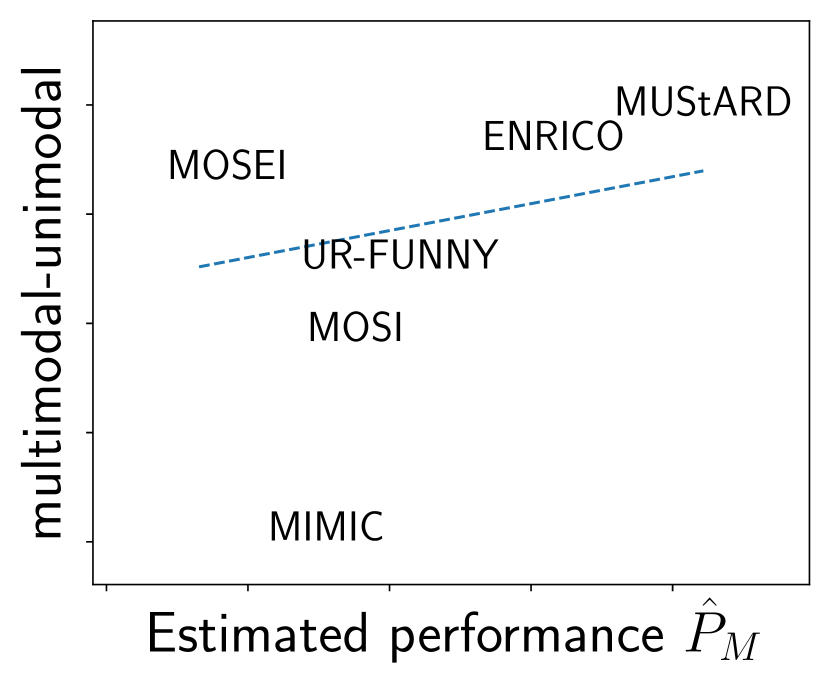
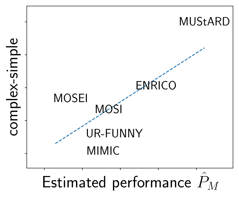
Figure 3: Datasets with higher estimated multimodal performance $\hat{P}_{M}$ tend to show improvements from unimodal to multimodal (left) and from simple to complex multimodal fusion (right).

RQ1: Should I collect multimodal data? We compare estimated performance $\hat{P}_{M}$ with the actual difference between unimodal and best multimodal performance in Figure 3 (left). Higher estimated $\hat{P}_{M}$ correlates with a larger gain from unimodal to multimodal. MUStARD and ENRICO show the most opportunity for multimodal modeling, but MIMIC shows less improvement.

RQ2: Should I investigate multimodal fusion? From Table 3, synergistic datasets like MUStARD and ENRICO show best reported multimodal performance only slightly above the estimated lower bound, indicating more work to be done in multimodal fusion. For datasets with less synergy like MOSEI and MIMIC, the best multimodal performance is much higher than the estimated lower bound, indicating that existing fusion methods may already be quite optimal. We compare $\hat{P}_{M}$ with the performance gap between complex and simple fusion methods in Figure 3 (right). We again observe trends between higher $\hat{P}_{M}$ and improvements with complex fusion, with large gains on MUStARD and ENRICO. We expect new methods to further improve the state-of-the-art on these datasets due to their generally high interaction values and low multimodal performance relative to estimated lower bound $\underline{P}_{\textrm{acc}}(f_{M}^{*})$.

4.3 Application 2: Self-supervised multimodal learning via disagreement

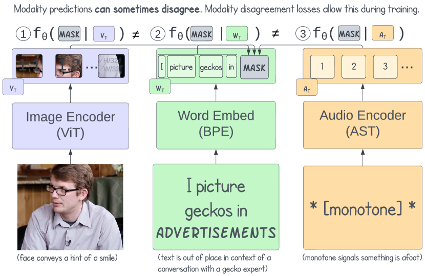
Figure 4: Masked predictions do not always agree across modalities, as shown in this example from the Social-IQ dataset [105]. Adding a slack term enabling pre-training with modality disagreement yields strong performance improvement over baselines.

Finally, we highlight an application of our analysis towards self-supervised pre-training, which is generally performed by encouraging agreement as a pre-training signal on large-scale unlabeled data [76, 81] before supervised fine-tuning [72]. However, our results suggest that there are regimes where disagreement can lead to synergy that may otherwise be ignored when only training for agreement. We therefore design a new family of self-supervised learning objectives that capture disagreement on unlabeled multimodal data.

Method: We build upon masked prediction that is popular in self-supervised pre-training: given multimodal data of the form $(x_{1},x_{2})\sim p(x_{1},x_{2})$ (e.g., $x_{1}=$ caption and $x_{2}=$ image), first mask out some words ($x_{1}^{\prime}$) before using the remaining words ($x_{1}\textbackslash x_{1}^{\prime}$) to predict the masked words via learning $f_{\theta}(x_{1}^{\prime}|x_{1}\textbackslash x_{1}^{\prime})$, as well as the image $x_{2}$ to predict the masked words via learning $f_{\theta}(x_{1}^{\prime}|x_{2})$ [81, 107]. In other words, maximizing agreement between $f_{\theta}(x_{1}^{\prime}|x_{1}\textbackslash x_{1}^{\prime})$ and $f_{\theta}(x_{1}^{\prime}|x_{2})$ in predicting $x_{1}^{\prime}$:

$$\mathcal{L}_{\textrm{agree}}=d(f_{\theta}(x_{1}^{\prime}|x_{1}\textbackslash x_{1}^{\prime}),x_{1}^{\prime})+d(f_{\theta}(x_{1}^{\prime}|x_{2}),x_{1}^{\prime})$$ (10)

for a distance $d$ such as cross-entropy loss for discrete word tokens. To account for disagreement, we allow predictions on the masked tokens $x_{1}^{\prime}$ from two different modalities $i,j$ to disagree by a slack variable $\lambda_{ij}$. We modify the objective such that each term only incurs a loss penalty if each distance $d(x,y)$ is larger than $\lambda$ as measured by a margin distance $d_{\lambda}(x,y)=\max(0,d(x,y)-\lambda)$:

$$\mathcal{L}_{\textrm{disagree}}=\mathcal{L}_{\textrm{agree}}+\sum_{1\leq i<j\leq 2}d_{\lambda_{ij}}(f_{\theta}(x_{1}^{\prime}|x_{i}),f_{\theta}(x_{1}^{\prime}|x_{j}))$$ (11)

These $\lambda$ terms are hyperparameters, quantifying the amount of disagreement we tolerate between each pair of modalities during cross-modal masked pretraining ($\lambda=0$ recovers full agreement). We show this visually in Figure 4 by applying it to masked pre-training on text, video, and audio using MERLOT Reserve [107], and also apply it to FLAVA [81] for images and text experiments (see extensions to $3$ modalities and details in Appendix D).

Setup: We choose four settings with natural disagreement: (1) UR-FUNNY: humor detection from $16,000$ TED talk videos [40], (2) MUsTARD: $690$ videos for sarcasm detection from TV shows [14], (3) Social IQ: $1,250$ multi-party videos testing social intelligence knowledge [105], and (4) Cartoon: matching $704$ cartoon images and captions [44].

Table 4: Allowing for disagreement during self-supervised masked pre-training yields performance improvements on these datasets. Over $10$ runs, improvements that are statistically significant are shown in bold ($p<0.05$).

	Social-IQ	UR-FUNNY	MUStARD	Cartoon
FLAVA [81], MERLOT Reserve [107]	$70.6\pm 0.6$	$80.0\pm 0.7$	$77.4\pm 0.8$	$38.6\pm 0.6$
+ disagreement	$\mathbf{71.1\pm 0.5}$	$\mathbf{80.7\pm 0.5}$	$\mathbf{78.1\pm 1.1}$	$39.3\pm 0.5$

Results: From Table 4, allowing for disagreement yields improvements on these datasets, with those on Social IQ, UR-FUNNY, MUStARD being statistically significant (p-value $<0.05$ over $10$ runs). By analyzing the value of $\lambda$ resulting in the best validation performance through hyperparameter search, we can analyze when disagreement helps for which datasets, datapoints, and modalities. On a dataset level, we find that disagreement helps for video/audio and video/text, improving accuracy by up to 0.6% but hurts for text/audio, decreasing the accuracy by up to 1%. This is in line with intuition, where spoken text is transcribed directly from audio for these monologue and dialog videos, but video can have vastly different information. In addition, we find more disagreement between text/audio for Social IQ, which we believe is because it comes from natural videos while the others are scripted TV shows with more agreement between speakers and transcripts.

We further analyze individual datapoints with disagreement. On UR-FUNNY, the moments when the camera jumps from the speaker to their presentation slides are followed by an increase in agreement since the video aligns better with the speech. In MUStARD, we observe disagreement between vision and text when the speaker’s face expresses the sarcastic nature of a phrase. This changes the meaning of the phrase, which cannot be inferred from text only, and leads to synergy. We include more qualitative examples including those on the Cartoon captioning dataset in Appendix D.

5 Related Work

Multivariate information theory: The extension of information theory to $3$ or more variables [97, 33, 85, 70, 86, 34] remains on open problem. Partial information decomposition (PID) [98] was proposed as a potential solution that satisfies several appealing properties [10, 38, 95, 98]. Today, PID has primarily found applications in cryptography [69, 50], neuroscience [74], physics [30], complex systems [82], and biology [18], but its application towards machine learning, in particular multimodality, is an exciting but untapped research direction. To the best of our knowledge, our work is the first to provide formal estimates of synergy in the context of unlabeled or unpaired multimodal data which is common in today’s self-supervised paradigm [64, 76, 81, 107].

Understanding multimodal models: Information theory is useful for understanding co-training [12, 5, 15], multi-view learning [89, 92, 88, 84], and feature selection [101], where redundancy is an important concept. Prior research has also studied multimodal models via additive or non-additive interactions [31, 83, 43], gradient-based approaches [93], or visualization tools [67]. This goal of quantifying and modeling multimodal interactions [66] has also motivated many successful learning algorithms, such as contrastive learning [54, 76], agreement and alignment [24, 63], factorized representations [91], as well as tensors and multiplicative interactions [104, 60, 51].

Disagreement-based learning has been used to estimate performance from unlabeled data [4, 52], active learning [21, 39], and guiding exploration in reinforcement learning [73, 79]. In multimodal learning, however, approaches have been primarily based on encouraging agreement in prediction [12, 24, 28, 84] or feature space [76, 72] in order to capture shared information. Our work has arrived at similar conclusions regarding the benefits of disagreement-based learning, albeit from different mathematical motivations and applications.

6 Conclusion

We proposed estimators of multimodal interactions when observing only labeled unimodal data and some unlabeled multimodal data, a general setting that encompasses many real-world constraints involving partially observable modalities, limited labels, and privacy concerns. Our key results draw new connections between multimodal interactions, the disagreement of unimodal classifiers, and min-entropy couplings. Future work should investigate more applications of multivariate information theory in designing self-supervised models, predicting multimodal performance, and other tasks involving feature interactions such as privacy-preserving and fair representation learning.

Appendix

Broader Impact

Multimodal semi-supervised models are ubiquitous in a range of real-world applications with only labeled unimodal data and naturally co-occurring multimodal data (e.g., unlabeled images and captions, video and corresponding audio) but when labeling them is time-consuming. This paper is our attempt at formalizing the learning setting of multimodal semi-supervised learning, allowing us to derive bounds on the information existing in multimodal semi-supervised datasets and what can be learned by models trained on these datasets. We do not foresee any negative broad impacts of our theoretical results, but we do note the following concerns regarding the potential empirical applications of these theoretical results in real-world multimodal datasets:

Biases: We acknowledge risks of potential biases surrounding gender, race, and ethnicity in large-scale multimodal datasets [13, 62], especially those collected in a semi-supervised setting with unlabeled and unfiltered images and captions [11]. Formalizing the types of bias in multimodal datasets and mitigating them is an important direction for future work.

Privacy: When making predictions from multimodal datasets with recorded human behaviors and medical data, there might be privacy risks of participants. Following best practices in maintaining the privacy and safety of these datasets, (1) these datasets have only been collected from public data that are consented for public release (creative commons license and following fair use guidelines of YouTube) [14, 40, 106], or collected from hospitals under strict IRB and restricted access guidelines [53], and (2) have been rigorously de-identified in accordance with Health Insurance Portability and Accountability Act such that all possible personal and protected information has been removed from the dataset [53]. Finally, we only use these datasets for research purposes and emphasize that any multimodal models trained to perform prediction should only be used for scientific study and should not in any way be used for real-world harm.

Appendix A Detailed proofs

A.1 Information decomposition

Partial information decomposition (PID) [98] decomposes of the total information 2 variables provide about a task $I(\{X_{1},X_{2}\};Y)$ into 4 quantities: redundancy $R$ between $X_{1}$ and $X_{2}$, unique information $U_{1}$ in $X_{1}$ and $U_{2}$ in $X_{2}$, and synergy $S$. Williams and Beer [98], who first proposed PIDs, showed that they should satisfy the following consistency equations:

$$R+U_{1} =I(X_{1};Y),$$ (12)

$$R+U_{2} =I(X_{2};Y),$$ (13)

$$U_{1}+S =I(X_{1};Y|X_{2}),$$ (14)

$$U_{2}+S =I(X_{2};Y|X_{1}),$$ (15)

$$R-S =I(X_{1};X_{2};Y).$$ (16)

We choose the PID definition by Bertschinger et al. [10], where redundancy, uniqueness, and synergy are defined by the solution to the following optimization problems:

$$R =\max_{q\in\Delta_{p}}I_{q}(X_{1};X_{2};Y)$$ (17)

$$U_{1} =\min_{q\in\Delta_{p}}I_{q}(X_{1};Y|X_{2})$$ (18)

$$U_{2} =\min_{q\in\Delta_{p}}I_{q}(X_{2};Y|X_{1})$$ (19)

$$S =I_{p}(\{X_{1},X_{2}\};Y)-\min_{q\in\Delta_{p}}I_{q}(\{X_{1},X_{2}\};Y)$$ (20)

where $\Delta_{p}=\{q\in\Delta:q(x_{i},y)=p(x_{i},y)\ \forall y,x_{i},i\in\{1,2\}\}$, $\Delta$ is the set of all joint distributions over $X_{1},X_{2},Y$, and the notation $I_{p}(\cdot)$ and $I_{q}(\cdot)$ disambiguates MI under joint distributions $p$ and $q$ respectively. The key difference in this definition of PID lies in optimizing $q\in\Delta_{p}$ to satisfy the marginals $q(x_{i},y)=p(x_{i},y)$, but relaxing the coupling between $x_{1}$ and $x_{2}$: $q(x_{1},x_{2})$ need not be equal to $p(x_{1},x_{2})$. The intuition behind this is that one should be able to infer redundancy and uniqueness given only access to separate marginals $p(x_{1},y)$ and $p(x_{2},y)$, and therefore they should only depend on $q\in\Delta_{p}$ which match these marginals. Synergy, however, requires knowing the coupling $p(x_{1},x_{2})$, and this is reflected in equation (20) depending on the full $p$ distribution.

A.2 Computing $q^{*}$, redundancy, and uniqueness

According to Bertschinger et al. [10], it suffices to solve for $q$ using the following max-entropy optimization problem $q^{*}=\operatorname*{arg\,max}_{q\in\Delta_{p}}H_{q}(Y|X_{1},X_{2})$, the same $q^{*}$ equivalently solves any of the remaining problems defined for redundancy, uniqueness, and synergy. This is a concave maximization problem with linear constraints. When $\mathcal{X}_{i}$ and $\mathcal{Y}$ are small and discrete, we can represent all valid distributions $q(x_{1},x_{2},y)$ as a set of tensors $Q$ of shape $|\mathcal{X}_{1}|\times|\mathcal{X}_{2}|\times|\mathcal{Y}|$ with each entry representing $Q[i,j,k]=p(X_{1}=i,X_{2}=j,Y=k)$. The problem then boils down to optimizing over valid tensors $Q\in\Delta_{p}$ that match the marginals $p(x_{i},y)$ for the objective function $H_{q}(Y|X_{1},X_{2})$. We rewrite conditional entropy as a KL-divergence [36], $H_{q}(Y|X_{1},X_{2})=\log|\mathcal{Y}|-KL(q||\tilde{q})$, where $\tilde{q}$ is an auxiliary product density of $q(x_{1},x_{2})\cdot\frac{1}{|\mathcal{Y}|}$ enforced using linear constraints: $\tilde{q}(x_{1},x_{2},y)=q(x_{1},x_{2})/|\mathcal{Y}|$. The KL-divergence objective is recognized as convex, allowing the use of conic solvers such as SCS [71], ECOS [25], and MOSEK [3].

Finally, optimizing over $Q\in\Delta_{p}$ that match the marginals can also be enforced through linear constraints: the 3D-tensor $Q$ summed over the second dimension gives $q(x_{1},y)$ and summed over the first dimension gives $q(x_{2},y)$, yielding the final optimization problem:

$$\operatorname*{arg\,max}_{Q,\tilde{Q}}KL(Q||\tilde{Q}),\quad\textrm{s.t.}\quad \tilde{Q}(x_{1},x_{2},y)=Q(x_{1},x_{2})/|\mathcal{Y}|,$$ (21)

$$\sum_{x_{2}}Q=p(x_{1},y),\sum_{x_{1}}Q=p(x_{2},y),Q\geq 0,\sum_{x_{1},x_{2},y}Q=1.$$ (22)

After solving this optimization problem, plugging $q^{*}$ into (17)-(19) yields the desired estimators for redundancy and uniqueness: $R=I_{q^{*}}(X_{1};X_{2};Y),U_{1}=I_{q^{*}}(X_{1};Y|X_{2}),U_{2}=I_{q^{*}}(X_{2};Y|X_{1})$, and more importantly, can be inferred from access to only labeled unimodal data $p(x_{1},y)$ and $p(x_{2},y)$. Unfortunately, $S$ is impossible to compute via equation (20) when we do not have access to the full joint distribution $p$, since the first term $I_{p}(X_{1},X_{2};Y)$ is unknown. Instead, we will aim to provide lower and upper bounds in the form $\underline{S}\leq S\leq\overline{S}$ so that we can have a minimum and maximum estimate on what synergy could be. Crucially, $\underline{S}$ and $\overline{S}$ should depend only on $\mathcal{D}_{1}$, $\mathcal{D}_{2}$, and $\mathcal{D}_{M}$ in the multimodal semi-supervised setting.

A.3 Lower bound on synergy via redundancy (Theorem 1)

We first restate Theorem 1 from the main text to obtain our first lower bound $\underline{S}_{\textrm{agree}}$ linking synergy to redundancy:

Theorem 6.

(Lower-bound on synergy via redundancy, same as Theorem 1) We can relate $S$ to $R$ as follows

$$\underline{S}_{\textrm{agree}}=R-I_{p}(X_{1};X_{2})+\min_{r\in\Delta_{p_{1,2,12}}}I_{r}(X_{1};X_{2}|Y)\leq S$$ (23)

where $\Delta_{p_{1,2,12}}=\{r\in\Delta:r(x_{1},x_{2})=p(x_{1},x_{2}),r(x_{i},y)=p(x_{i},y)\}$. $\min_{r\in\Delta_{p_{1,2,12}}}I_{r}(X_{1};X_{2}|Y)$ is a max-entropy convex optimization problem which can be solved exactly using linear programming.

Proof.

By consistency equation (16) $S=R-I_{p}(X_{1};X_{2};Y)=R-I_{p}(X_{1};X_{2})+I_{p}(X_{1};X_{2}|Y)$. This means that lower bounding the synergy is the same as obtaining a lower bound on the mutual information $I_{p}(X_{1},X_{2}|Y)$, since $R$ and $I_{p}(X_{1};X_{2})$ can be computed exactly based on $p(x_{1},y)$, $p(x_{2},y)$, and $p(x_{1},x_{2})$. To lower bound $I_{p}(X_{1},X_{2}|Y)$, we consider minimizing it subject to the marginal constraints with $p$, which gives

$$\min_{r\in\Delta_{p_{1,2,12}}}I_{r}(X_{1};X_{2}|Y) =\min_{r\in\Delta_{p_{1,2,12}}}H_{r}(X_{1})-I_{r}(X_{1};Y)-H_{r}(X_{1}|X_{2},Y)$$ (24)

$$=H_{p}(X_{1})-I_{p}(X_{1};Y)-\max_{r\in\Delta_{p_{1,12}}}H_{r}(X_{1}|X_{2},Y)$$ (25)

where in the last line the $p_{2}$ constraint is removed since $H_{r}(X_{1}|X_{2},Y)$ is fixed with respect to $p(x_{2},y)$. To solve $\max_{r\in\Delta_{p_{1,12}}}H_{r}(X_{1}|X_{2},Y)$, we observe that it is also a concave maximization problem with linear constraints. When $\mathcal{X}_{i}$ and $\mathcal{Y}$ are small and discrete, we can represent all valid distributions $r(x_{1},x_{2},y)$ as a set of tensors $R$ of shape $|\mathcal{X}_{1}|\times|\mathcal{X}_{2}|\times|\mathcal{Y}|$ with each entry representing $R[i,j,k]=p(X_{1}=i,X_{2}=j,Y=k)$. The problem then boils down to optimizing over valid tensors $R\in\Delta_{p_{1,12}}$ that match the marginals $p(x_{1},y)$ and $p(x_{1},x_{2})$. Given a tensor $R$ representing $r$, our objective is the concave function $H_{r}(X_{1}|X_{2},Y)$ which we rewrite as a KL-divergence $\log|\mathcal{X}_{1}|-KL(r||\tilde{r})$ using an auxiliary distribution $\tilde{r}=r(x_{2},y)\cdot\frac{1}{|\mathcal{X}_{1}|}$ and solve it exactly using convex programming with linear constraints:

$$\operatorname*{arg\,max}_{R,\tilde{R}}KL(R||\tilde{R}),\quad\textrm{s.t.}\quad \tilde{R}(x_{1},x_{2},y)=R(x_{2},y)/|\mathcal{Y}|,$$ (26)

$$\sum_{x_{2}}R=p(x_{1},y),\sum_{y}R=p(x_{1},x_{2}),R\geq 0,\sum_{x_{1},x_{2},y}R=1.$$ (27)

with marginal constraints $R\in\Delta_{p_{1,12}}$ enforced through linear constraints on tensor $R$. Plugging the optimized $r^{*}$ into (23) yields the desired lower bound $\underline{S}_{\textrm{agree}}=R-I_{p}(X_{1};X_{2})+I_{r^{*}}(X_{1};X_{2}|Y)$. ∎

A.4 Lower bound on synergy via disagreement (Theorem 2)

We first restate some notation and definitions from the main text for completeness. The key insight behind Theorem 2, a relationship between disagreement and synergy, is that while labeled multimodal data is unavailable, the output of unimodal classifiers may be compared against each other. Let $\delta_{\mathcal{Y}}=\{r\in\mathbb{R}_{+}^{|\mathcal{Y}|}\ |\ ||r||_{1}=1\}$ be the probability simplex over labels $\mathcal{Y}$. Consider the set of unimodal classifiers $\mathcal{F}_{i}\ni f_{i}:\mathcal{X}_{i}\rightarrow\delta_{\mathcal{Y}}$ and multimodal classifiers $\mathcal{F}_{M}\ni f_{M}:\mathcal{X}_{1}\times\mathcal{X}_{2}\rightarrow\delta_{\mathcal{Y}}$.

Definition 3.

(Unimodal and multimodal loss) The loss of a given unimodal classifier $f_{i}\in\mathcal{F}_{i}$ is given by $L(f_{i})=\mathbb{E}_{p(x_{i},y)}\left[\ell(f_{i}(x_{i}),y)\right]$ for a loss function over the label space $\ell:\mathcal{Y}\times\mathcal{Y}\rightarrow\mathbb{R}^{\geq 0}$. We denote the same for multimodal classifier $f_{M}\in\mathcal{F}_{M}$, with a slight abuse of notation $L(f_{M})=\mathbb{E}_{p(x_{1},x_{2},y)}\left[\ell(f_{M}(x_{1},x_{2}),y)\right]$ for a loss function over the label space $\ell$.

Definition 4.

(Unimodal and multimodal accuracy) The accuracy of a given unimodal classifier $f_{i}\in\mathcal{F}_{i}$ is given by $P_{\textrm{acc}}(f_{i})=\mathbb{E}_{p}\left[\mathbf{1}\left[f_{i}(x_{i})=y\right]\right]$. We denote the same for multimodal classifier $f_{M}\in\mathcal{F}_{M}$, with a slight abuse of notation $P_{\textrm{acc}}(f_{M})=\mathbb{E}_{p}\left[\mathbf{1}\left[f_{M}(x_{1},x_{2})=y\right]\right]$.

An unimodal classifier $f_{i}^{*}$ is Bayes-optimal (or simply optimal) with respect to a loss function $L$ if $L(f_{i}^{*})\leq L(f^{\prime}_{i})$ for all $f^{\prime}_{i}\in\mathcal{F}_{i}$. Similarly, a multimodal classifier $f_{M}^{*}$ is optimal with respect to loss $L$ if $L(f_{M}^{*})\leq L(f^{\prime}_{M})$ for all $f^{\prime}_{M}\in\mathcal{F}_{M}$.

Bayes optimality can also be defined with respect to accuracy, if $P_{\textrm{acc}}(f_{i}^{*})\geq P_{\textrm{acc}}(f^{\prime}_{i})$ for all $f^{\prime}_{i}\in\mathcal{F}_{i}$ for unimodal classifiers, or if $P_{\textrm{acc}}(f_{M}^{*})\geq P_{\textrm{acc}}(f^{\prime}_{M})$ for all $f^{\prime}_{M}\in\mathcal{F}_{M}$ for multimodal classifiers.

The crux of our method is to establish a connection between modality disagreement and a lower bound on synergy.

Definition 5.

(Modality disagreement) Given $X_{1}$, $X_{2}$, and a target $Y$, as well as unimodal classifiers $f_{1}$ and $f_{2}$, we define modality disagreement as $\alpha(f_{1},f_{2})=\mathbb{E}_{p(x_{1},x_{2})}[d(f_{1},f_{2})]$ where $d:\mathcal{Y}\times\mathcal{Y}\rightarrow\mathbb{R}^{\geq 0}$ is a distance function in label space scoring the disagreement of $f_{1}$ and $f_{2}$’s predictions,

where the distance function $d$ must satisfy some common distance properties, following Sridharan and Kakade [84]:

Assumption 1.

(Relaxed triangle inequality) For the distance function $d:\mathcal{Y}\times\mathcal{Y}\rightarrow\mathbb{R}^{\geq 0}$ in label space scoring the disagreement of $f_{1}$ and $f_{2}$’s predictions, there exists $c_{d}\geq 1$ such that

$$\forall\hat{y}_{1},\hat{y}_{2},\hat{y}_{3}\in\hat{\mathcal{Y}},\quad d(\hat{y}_{1},\hat{y}_{2})\leq c_{d}\left(d(\hat{y}_{1},\hat{y}_{3})+d(\hat{y}_{3},\hat{y}_{2})\right).$$ (28)

Assumption 2.

(Inverse Lipschitz condition) For the function $d$, it holds that for all $f$,

$$\mathbb{E}[d(f(x_{1},x_{2}),f^{*}(x_{1},x_{2}))]\leq|L(f)-L(f^{*})|$$ (29)

where $f^{*}$ is the Bayes optimal multimodal classifier with respect to loss $L$, and

$$\mathbb{E}[d(f_{i}(x_{i}),f_{i}^{*}(x_{i}))]\leq|L(f_{i})-L(f_{i}^{*})|$$ (30)

where $f_{i}^{*}$ is the Bayes optimal unimodal classifier with respect to loss $L$.

Assumption 3.

(Classifier optimality) For any unimodal classifiers $f_{1},f_{2}$ in comparison to the Bayes’ optimal unimodal classifiers $f_{1}^{*},f_{2}^{*}$, there exists constants $\epsilon_{1},\epsilon_{2}>0$ such that

$$|L(f_{1})-L(f_{1}^{*})|^{2}\leq\epsilon_{1},|L(f_{2})-L(f_{2}^{*})|^{2}\leq\epsilon_{2}$$ (31)

We now restate Theorem 2 from the main text obtaining $\underline{S}_{\textrm{disagree}}$, our second lower bound on synergy linking synergy to disagreement:

Theorem 7.

(Lower-bound on synergy via disagreement, same as Theorem 2) We can relate synergy $S$ and uniqueness $U$ to modality disagreement $\alpha(f_{1},f_{2})$ of optimal unimodal classifiers $f_{1},f_{2}$ as follows:

$$\underline{S}_{\textrm{disagree}}=\alpha(f_{1},f_{2})\cdot c-\max(U_{1},U_{2})\leq S$$ (32)

for some constant $c$ depending on the label dimension $|\mathcal{Y}|$ and choice of label distance function $d$.

Theorem 7 implies that if there is substantial disagreement between the unimodal classifiers $f_{1}$ and $f_{2}$, it must be due to the presence of unique or synergistic information. If uniqueness is small, then disagreement must be accounted for by the presence of synergy, which yields a lower bound.

Proof.

The first part of the proof is due to an intermediate result by Sridharan and Kakade [84], which studies how multi-view agreement can help train better multiview classifiers. We restate the key proof ideas here for completeness. The first step is to relate $I_{p}(X_{2};Y|X_{1})$ to $|L(f_{1}^{*})-L(f^{*})|^{2}$, the difference in errors between the Bayes’ optimal unimodal classifier $f_{1}^{*}$ with the Bayes’ optimal multimodal classifier $f^{*}$ for some appropriate loss function $L$ on the label space:

$$|L(f_{1}^{*})-L(f^{*})|^{2} =|\mathbb{E}_{X}\mathbb{E}_{Y|X_{1},X_{2}}\ell(f^{*}(x_{1},x_{2}),y)-\mathbb{E}_{X}\mathbb{E}_{Y|X_{1}}\ell(f^{*}(x_{1},x_{2}),y)|^{2}$$ (33)

$$\leq|\mathbb{E}_{Y|X_{1},X_{2}}\ell(f^{*}(x_{1},x_{2}),y)-\mathbb{E}_{Y|X_{1}}\ell(f^{*}(x_{1},x_{2}),y)|^{2}$$ (34)

$$\leq\textrm{KL}(p(y|x_{1},x_{2}),p(y|x_{1}))$$ (35)

$$\leq\mathbb{E}_{X}\textrm{KL}(p(y|x_{1},x_{2}),p(y|x_{1}))$$ (36)

$$=I_{p}(X_{2};Y|X_{1}),$$ (37)

where we used Pinsker’s inequality in (35) and Jensen’s inequality in (36). Symmetrically, $|L(f_{2}^{*})-L(f^{*})|^{2}\leq I_{p}(X_{1};Y|X_{2})$, and via the triangle inequality through the Bayes’ optimal multimodal classifier $f^{*}$ and the inverse Lipschitz condition we obtain

$$\mathbb{E}_{p(x_{1},x_{2})}[d(f_{1}^{*},f_{2}^{*})] \leq\mathbb{E}_{p(x_{1},x_{2})}[d(f_{1}^{*},f^{*})]+\mathbb{E}_{p(x_{1},x_{2})}[d(f^{*},f_{2}^{*})]$$ (38)

$$\leq|L(f_{1}^{*})-L(f^{*})|^{2}+|L(f_{2}^{*})-L(f^{*})|^{2}$$ (39)

$$\leq I_{p}(X_{2};Y|X_{1})+I_{p}(X_{1};Y|X_{2}).$$ (40)

Next, we relate disagreement $\alpha(f_{1},f_{2})$ to $I_{p}(X_{2};Y|X_{1})$ and $I_{p}(X_{1};Y|X_{2})$ via the triangle inequality through the Bayes’ optimal unimodal classifiers $f_{1}^{*}$ and $f_{2}^{*}$:

$$\alpha(f_{1},f_{2}) =\mathbb{E}_{p(x_{1},x_{2})}[d(f_{1},f_{2})]$$ (41)

$$\leq c_{d}\left(\mathbb{E}_{p(x_{1},x_{2})}[d(f_{1},f_{1}^{*})]+\mathbb{E}_{p(x_{1},x_{2})}[d(f_{1}^{*},f_{2}^{*})]+\mathbb{E}_{p(x_{1},x_{2})}[d(f_{2}^{*},f_{2})]\right)$$ (42)

$$\leq c_{d}\left(\epsilon_{1}^{\prime}+I_{p}(X_{2};Y|X_{1})+I_{p}(X_{1};Y|X_{2})+\epsilon_{2}^{\prime}\right)$$ (43)

$$\leq 2c_{d}(\max(I_{p}(X_{1};Y|X_{2}),I_{p}(X_{2};Y|X_{1}))+\max(\epsilon_{1}^{\prime},\epsilon_{2}^{\prime}))$$ (44)

where used classifier optimality assumption for unimodal classifiers $f_{1},f_{2}$ in (43). Finally, we use consistency equations of PID relating $U$ and $S$ in (14)-(15): to complete the proof:

$$\alpha(f_{1},f_{2}) \leq 2c_{d}(\max(I_{p}(X_{1};Y|X_{2}),I_{p}(X_{2};Y|X_{1}))+\max(\epsilon_{1}^{\prime},\epsilon_{2}^{\prime}))$$ (45)

$$=2c_{d}(\max(U_{1}+S,U_{2}+S)+\max(\epsilon_{1}^{\prime},\epsilon_{2}^{\prime}))$$ (46)

$$=2c_{d}(S+\max(U_{1},U_{2})+\max(\epsilon_{1}^{\prime},\epsilon_{2}^{\prime})),$$ (47)

In practice, setting $f_{1}$ and $f_{2}$ as neural network function approximators that can achieve the Bayes’ optimal risk [45] results in $\max(\epsilon_{1}^{\prime},\epsilon_{2}^{\prime})=0$, and rearranging gives us the desired inequality. ∎

A.5 Proof of NP-hardness (Theorem 3)

Our proof is based on a reduction from the restricted timetable problem, a well-known scheduling problem closely related to constrained edge coloring in bipartite graphs. Our proof description proceeds along 4 steps.

1. Description of our problem.

2. How the minimum entropy objective can engineer “classification” problems using a technique from Kovačević et al. [56].

3. Description of the RTT problem of Even et al. [26], how to visualize RTT as a bipartite edge coloring problem, and a simple variant we call $Q$-RTT which RTT reduces to.

4. Polynomial reduction of $Q$-RTT to our problem.

A.5.1 Formal description of our problem

Recall that our problem was

$$\min_{r\in\Delta_{p_{1,2,12}}}H_{r}(X_{1},X_{2},Y)$$

where $\Delta_{p_{1,2,12}}=\{r\in\Delta:r(x_{1},x_{2})=p(x_{1},x_{2}),r(x_{i},y)=p(x_{i},y)\}$. Our goal is to find the minimum-entropy distribution over $\mathcal{X}_{1}\times\mathcal{X}_{2}\times\mathcal{Y}$ where the pairwise marginals over $(X_{1},X_{2})$, $(X_{1},Y)$ and $(X_{2},Y)$ are specified as part of the problem. Observe that this description is symmetrical, $X_{i}$ and $Y$ could be swapped without loss of generality.

A.5.2 Warm up: using the min-entropy objective to mimic multiclass classification

We first note the strong similarity of our min-entropy problem to the classic min-entropy coupling problem in two variables. There where the goal is to find the min-entropy joint distribution over $\mathcal{X}\times\mathcal{Y}$ given fixed marginal distributions of $p(x)$ and $p(y)$. This was shown to be an NP-hard problem which has found many practical applications in recent years. An approximate solution up to $1$ bit can be found in polynomial time (and is in fact the same approximation we give to our problem). Our NP-hardness proof involves has a similar flavor as [56], which is based on a reduction from the classic subset sum problem, exploiting the min-entropy objective to enforce discrete choices.

Subset sum

There are $d$ items with value $c_{1}\dots c_{d}\geq 0$, which we assume WLOG to be normalized such that $\sum_{i}^{d}c_{i}=1$. Our target sum is $0\leq T\leq 1$. The goal is to find if some subset $\mathcal{S}\subseteq[d]$ exists such that $\sum_{i\in\mathcal{S}}c_{i}=T$.

Reduction from subset sum to min-entropy coupling [56]

Let $\mathcal{X}$ be the $d$ items and $\mathcal{Y}$ be binary, indicating whether the item was chosen. Our joint distribution is of size $|\mathcal{X}|\times|\mathcal{Y}|$. We set the following constraints on marginals.

1. $p(x_{i})=c_{i}$ for all $i$, (row constraints)

2. $p(\text{include})=T$, $p(\text{omit})=1-T$, (column constraints)

Constraints (i) split the value of each item additively into nonnegative components to be included and not included from our chosen subset, while (ii) enforces that the items included sum to $T$. Observe that the min-entropy objective $H(X,Y)=H(Y|X)+H(X)$, which is solely dependent on $H(Y|X)$ since $H(X)$ is a constant given marginal constraints on $X$. Thus, $H(Y|X)$ is nonnegative and is only equal to 0 if and only if $Y$ is deterministic given $X$, i.e., $r(x_{i},\text{include})=0$ or $r(x_{i},\text{omit})=0$. If our subset sum problem has a solution, then this instantiation of the min-entropy coupling problem would return a deterministic solution with $H(Y|X)=0$, which in turn corresponds to a solution in subset sum. Conversely, if subset sum has no solution, then our min-entropy coupling problem is either infeasible OR gives solutions where $H(Y|X)>0$ strictly, i.e., $Y|X$ is non-deterministic, which we can detect and report.

Relationship to our problem

Observe that our joint entropy objective may be decomposed

$$H_{r}(X_{1},X_{2},Y)=H_{r}(Y|X_{1},X_{2})+H_{r}(X_{1},X_{2}).$$

Given that $p(x_{1},x_{2})$ is fixed under $\Delta_{p_{1,2,12}}$, our objective is equivalent to minimizing $H_{r}(Y|X_{1},X_{2})$. Similar to before, we know that $H_{r}(Y|X_{1},X_{2})$ is nonnegative and equal to zero if and only if $Y$ is deterministic given $(X_{1},X_{2})$.

Intuitively, we can use $\mathcal{X}_{1},\mathcal{X}_{2}$ to represent vertices in a bipartite graph, such that $(X_{1},X_{2})$ are edges (which may or may not exist), and $\mathcal{Y}$ as colors for the edges. Then, the marginal constraints for $p(x_{1},x_{2})$ could be used alongside the min-entropy objective to ensure that each edge has exactly one color. The marginal constraints $p(x_{1},y)$ and $p(x_{2},y)$ tell us (roughly speaking) the number of edges of each color that is adjacent to vertices in $\mathcal{X}_{1}$ and $\mathcal{X}_{2}$.

However, this insight alone is not enough; first, edge coloring problems in bipartite graphs (e.g., colorings in regular bipartite graphs) can be solved in polynomial time, so we need a more difficult problem. Second, we need an appropriate choice of marginals for $p(x_{i},y)$ that does not immediately ‘reveal’ the solution. Our proof uses a reduction from the restricted timetable problem, one of the most primitive scheduling problems available (and closely related to edge coloring or multicommodity network flow).

A.5.3 Restricted Timetable Problem (RTT)

The restricted timetable (RTT) problem was introduced by Even et al. [26], and has to do with how to schedule teachers to classes they must teach. It comprises the following

• A collection of $\{T_{1},\dots,T_{n}\}$, where $T_{i}\subseteq[3]$. These represent $n$ teachers, each of which is available for the hours given in $T_{i}$.

• $m$ students, each of which is available at any of the $3$ hours

• An binary matrix $\{0,1\}^{n\times m}$. $R_{ij}=1$ if teacher $i$ is required to teach class $j$, and $0$ otherwise. Since $R_{ij}$ is binary, each class is taught by a teacher at most once.

• Each teacher is tight, i.e., $|T_{i}|=\sum_{j=1}^{m}R_{ij}$. That is, every teacher must teach whenever they are available.

Suppose there are exactly 3 hours a day. The problem is to determine if there exists a meeting function

$$f:[n]\times[m]\times[3]\rightarrow\{0,1\},$$

where our goal is to have $f(i,j,h)=1$ if and only if teacher $i$ teaches class $j$ at the $h$-th hour. We require the following conditions in our meeting function:

1. $f(i,j,h)=1\implies h\in T_{i}$. This implies that teachers are only teaching in the hours they are available.

2. $\sum_{h\in[3]}f(i,j,h)=R_{ij}$ for all $i\in[n],j\in[m]$. This ensures that every class gets the teaching they are required, as specified by $R$.

3. $\sum_{i\in[n]}f(i,j,h)\leq 1$ for all $j\in[m]$ and $h\in[3]$. This ensures no class is taught by more than one teachers at once.

4. $\sum_{j\in[m]}f(i,j,h)\leq 1$ for all $i\in[n]$ and $h\in[3]$. This ensures no teacher is teaching more than one class simultaneously.

Even et al. [26] showed that RTT is NP-hard via a clever reduction from 3-SAT. Our strategy is to reduce RTT to our problem.

(a) Valid coloring

(b) Invalid: class 1 used repeated color (blue)

(c) Invalid: teacher 1 used repeated color (green)

(d) Invalid: teacher 2 used invalid color (green)

Figure 5: Examples of valid and invalid colorings. Left vertices are teachers 1, 2, 3. Right vertices are classes 1, 2. The colors red, green, blue are for hours 1, 2, 3 respectively, color of teacher vertices are the hours where the teachers are available (by definition of RTT, the number of distinct colors per teacher vertex is equal to its degree). The color of an edge (red, green or blue) says that a teacher is assigned to that class at that hour. Figure 5(a) shows a valid coloring (or timetabling), since (i) all edges are colored, (ii) no edge of the same colors are adjacent, and (iii) edges adjacent to teachers correspond to the vertex’s color. Figures 5(b), 5(c), 5(d) are invalid colorings because of same-colored edges being adjacent, or teacher vertex colors differing to adjacent edges.

Viewing RTT through the lens of bipartite edge coloring

RTT can be visualized as a variant of constrained edge coloring in bipartite graphs (Figure 5). The teachers and classes are the two different sets of vertices, while $R$ gives the adjacency structure. There are 3 colors available, corresponding to hours in a day. The task is to color the edges of the graph with these $3$ colors such that

1. No two edges of the same color are adjacent. This ensures students and classes are at most teaching/taking one session at any given hour (condition 3 and 4)

2. Edges adjacent to teacher $i$ are only allowed colors in $T_{i}$. This ensures teachers are only teaching in available hours (condition 1)

If every edge is colored while obeying the above conditions, then it follows from the tightness of teachers (in the definition of RTT) that every class is assigned their required lessons (condition 2). The decision version of the problem is to return if such a coloring is possible.

Time Constrained RTT ($Q$-RTT)

A variant of RTT that will be useful is when we impose restrictions on the number of classes being taught at any each hour. We call this $Q$-RTT, where $Q=(q_{1},q_{2},q_{3})\in\mathbb{Z}^{3}$. $Q$-RTT returns true if, in addition to the usual RTT conditions, we require the meeting function to satisfy

$$\sum_{i\in[n],j\in[m]}f(i,j,h)=q_{h}.$$

That is, the total number of hours taught by teachers in hour $h$ is exactly $q_{h}$. From the perspective of edge coloring, $Q$-RTT simply imposes an additional restriction on the total number of edges of each color, i.e., there are $q_{k}$ edges of color $k$ for each $k\in[3]$.

Obviously, RTT can be Cook reduced to $Q$-RTT: since there are only $3$ hours and a total of $g=\sum_{i\in[n],j\in[m]}R_{ij}$ total lessons to be taught, there are at most $\mathcal{O}(g^{2})$ ways of splitting the required number of lessons up amongst the 3 hours. Thus, we can solve RTT by making at most $\mathcal{O}(g^{2})$ calls to $Q$-RTT. This is polynomial in the size of RTT, and we conclude $Q$-RTT is NP-hard.

A.5.4 Reduction of $Q$-RTT to our problem

We will reduce $Q$-RTT to our problem. Let $\alpha=1/\left(\sum_{i,j}R_{ij}+3m\right)$, where $1/\alpha$ should be seen as a normalizing constant given by the number of edges in a bipartite graph. One should think of $\alpha$ as an indicator of the boolean TRUE and $0$ as FALSE. We use the following construction

1. Let $\mathcal{X}_{1}=[n]\cup\mathcal{Z}$, where $\mathcal{Z}=\{Z_{1},Z_{2},Z_{3}\}$. From a bipartite graph interpretation, these form one set of vertices that we will match to classes. $Z_{1},Z_{2},Z_{3}$ are “holding rooms”, one for each of the 3 hours. Holding rooms are like teachers whose classes can be assigned in order to pass the time. They will not fulfill any constraints on $R$, but they can accommodate multiple classes at once. We will explain the importance of these holding rooms later.

2. Let $\mathcal{X}_{2}=[m]$. These form the other set of vertices, one for each class.

3. Let $\mathcal{Y}=[3]\cup\{0\}$. 1, 2, and 3 are the 3 distinct hours, corresponding to edge colors. 0 is a special “null” color which will only be used when coloring edges adjacent to the holding rooms.

4. Let $p(i,j,\cdot)=\alpha\cdot R_{ij}$ and $p(i,j)=\alpha$ for all $i\in\mathcal{Z}$, $j\in[m]$. Essentially, there is an edge between a teacher and class if $R$ dictates it. There are also always edges from every holding room to each class.

5. For $i\in[n]$, set $p(i,\cdot,h)=\alpha$ if $h\in T_{i}$, $0$ otherwise. For $Z_{i}\in\mathcal{Z}$, we set

   $$p(Z_{i},\cdot,h)=\begin{cases}\alpha\cdot q_{i}\quad&h=0\\ \alpha\cdot(m-q_{i})\quad&h=i\\ 0\quad&\text{otherwise}\end{cases}$$

   In order words, at hour $h$, when a class is not assigned to some teacher (which would to contribute to $q_{h}$), they must be placed in holding room $Z_{h}$.

6. Let $p(\cdot,j,h)=\alpha$ for $h\in[3]$, and $p(\cdot,j,h)=\alpha\cdot\sum_{i\in[n]}R_{i,j}$. The former constraint means that for each of the 3 hours, the class must be taking some lesson with a teacher OR in the holding room. The second constraint assigns the special “null” value to the holding rooms which were not used by that class.

(a) Valid coloring

(b) Invalid: class 1 used repeated color (blue)

(c) Invalid: teacher 1 used repeated color (green)

(d) Invalid: teacher 2 used invalid color (green)

Figure 6: Examples of valid and invalid colorings when holding rooms are included. For simplicity, we illustrate all constraints except those on $Q$. Left vertices are teachers 1, 2, 3 and holding rooms $Z_{1},Z_{2},Z_{3}$. Right vertices are classes 1, 2. The colors red, green, blue are for hours 1, 2, 3 respectively, color of teacher vertices are the hours where the teachers are available (by definition of RTT, the number of distinct colors per teacher vertex is equal to its degree). Border color of holding room vertices are the hour that the holding room is available. The color of an edge (red, green or blue) says that a teacher (or holding room) is assigned to that class at that hour. Gray edges are the “null” color, meaning that that waiting room is not used by that class. Figure 6(a) shows a valid coloring (or timetabling), since all edges are colored, no edge of the same colors are adjacent (other than the gray ones), and edges adjacent to teachers correspond to the vertex’s color. Figures 6(b), 6(c), 6(d) are invalid colorings because of non-gray edges being adjacent, or teacher vertices being adjacent to colors different from itself.

A solution to our construction with 0 conditional entropy implies a valid solution to $Q$-RTT

Suppose that our construction returns a distribution $r$ such that every entry $r(x_{1},x_{2},y)$ is either $\alpha$ or $0$. We claim that the meeting function $f(i,j,h)=1$ if $r(i,j,h)=\alpha$ and $0$ otherwise solves $Q$-RTT.

• Teachers are only teaching in the hours they are available, because of our marginal constraint on $p(i,\cdot,h)$.

• Every class gets the teaching they need. This follows from the fact that teachers are tight and the marginal constraint $p(i,\cdot,h)$, which forces teachers to be teaching whenever they can. The students are getting the lessons from the right teachers because of the marginal constraint on $p(i,j,\cdot)$, since teachers who are not supposed to teach a class have those marginal values set to $0$.

• No class is taught by more than one teacher at once. This follows from marginal constraint $p(\cdot,j,h)$. For each of the hours, a class is with either a single teacher or the holding room.

• No teacher is teaching more than one class simultaneously. This holds again from our marginal constraint on $p(i,\cdot,h)$.

• Lastly, the total number of lessons (not in holding rooms) held in each hour is $q_{h}$ as required by $Q$-RTT. To see why, we consider each color (hour). Each color (excluding the null color) is used exactly $m$ times by virtue of $p(\cdot,j,h)$. Some of these are in holding rooms, other are with teachers. The former (over all classes) is given by $m-q_{h}$ because of our constraint on $p(i,\cdot,h)$, which means that exactly $q_{h}$ lessons in hour $h$ as required.

A valid solution to $Q$-RTT implies a solution to our construction with 0 conditional entropy

Given a solution to $Q$-RTT, we recover a candidate solution to our construction in a natural way. If teacher $i$ is teaching class $j$ in hour $h$, then color edge $ij$ with color $h$, i.e., $r(i,j,h)=\alpha$ and $r(i,j,h^{\prime})=0$ if $h^{\prime}\neq h$. Since in RTT each teacher and class can be assigned one lesson per hour at most, there will be no clashes with this assignment. For all other $i\in[3],j\in[m]$ where $R_{ij}=0$, we assign $r(i,j,\cdot)=0$. Now, we will also need to assign students to holding rooms. For $h\in[3]$, we set $r(Z_{h},j,h)=\alpha$ if class $j$ was not assigned to any teacher in hour $h$. If class $j$ was assigned some teacher in hour $h$, then $r(Z_{h},j,0)=\alpha$, i.e., we give it the special null color. All other entries are given a value of $0$. We can verify

• $r$ is a valid probability distribution. The nonnegativity of $r$ follows from the fact that $\alpha>0$ strictly. We need to check that $r$ sums to $1$. We break this down into two cases based on whether the first argument of $r$ is some $Z_{h}$ or $i$. In Case 1, we have

  $$\sum_{i\in[n],h\in[3]\cup\{0\},j\in[m]}r(i,j,h)= \sum_{i\in[n],h\in[3],j\in[m]}r(i,j,h)$$

  $$= \alpha\cdot\sum_{i\in[n],j\in[m]}R_{ij},$$

  where the first line follows from the fact that we never color a teacher-class edge with the null color, and the second line is because every class gets its teaching requirements satisfied. In Case 2, we know that by definition every class is matched to every holding room and assigned either the null color or that room’s color, hence

  $$\sum_{i\in\{Z_{1},Z_{2},Z_{3}\},h\in[3]\cup\{0\},j\in[m]}r(i,j,h)= 3m$$

  Summing them up, we have $\alpha\cdot\left(3m+\sum_{i\in[n],j\in[m]}R_{ij}\right)=1$ (by our definition of $\alpha$.

• This $r$ distribution has only entries in $\alpha$ or $0$. This follows by definition.

• This $r$ distribution has minimum conditional entropy. For a fixed $i,j$, $r(i,j,\cdot)$ is either $\alpha$ or $0$. That is, $Y$ is deterministic given $X_{1},X_{2}$, hence $H(Y|X_{1},X_{2})=0$.

• All 3 marginal constraints in our construction are obeyed. We check them in turn.

  • Marginal constraint $r(i,j)=p(i,j)$. When $i\in[3]$: (i) when $R_{ij}=1$ exactly one time $h$ is assigned to teacher $i$ and class $j$, hence $r(i,j)=\alpha=p(i,j)$ as required, (ii)when $R_{ij}=0$ as specified. Now when $i\in\{Z_{1},Z_{2},Z_{3}\}$, we have $r(i,j,\cdot)=\alpha=p(i,j)$ since every holding room is either assigned it’s color to a class, or assigned the special null color.

  • Marginal constraint $r(i,h)=p(i,h)$. When $i\in[3]$, this follows directly from tightness. Similarly, when $i\in\{Z_{1},Z_{2},Z_{3}\}$, we have by definition of $Q$-RTT the assignments to holding rooms equal to $m-q_{h}$ for hour $h$, and consequently, $q_{h}$ null colors adjacent to $Z_{h}$ as required.

  • Marginal constraint $r(j,h)=p(j,h)$. For every $h\in[3]$, the class is assigned either to a teacher or a holding room, so this is equal to $\alpha$ as required. For $h=0$, i.e., the null color, this is used exactly $\sum_{i\in[n]}R_{ij}$ times (since these were the number hours that were not assigned to teachers), as required, making its marginal $\sum_{i\in[n]}R_{ij}$ and $r(j,h)=\alpha\cdot\sum_{i\in[n]}R_{ij}$ as required.

Thus, if RTT returns TRUE, our construction will also return a solution with entries in $\{0,\alpha\}$, and vice versa.

Corollary

The decision problem of whether there exists a distribution in $r\in\Delta_{p_{1,2,12}}$ such that $H(Y|X_{1},X_{2})=0$ is NP-complete. This follows because the problem is in NP since checking if $Y$ is deterministic (i.e., $H(Y|X_{1},X_{2})=0$) can be done in polynomial time, while NP-hardness follows from the same argument as above.

A.6 Upper bound on synergy (Theorem 4)

We begin by restating Theorem 4 from the main text:

Theorem 8.

(Upper-bound on synergy, same as Theorem 4).

$$S\leq H_{p}(X_{1},X_{2})+H_{p}(Y)-\min_{r\in\Delta_{p_{12,y}}}H_{r}(X_{1},X_{2},Y)-\max_{q\in\Delta_{p_{1,2}}}I_{q}(\{X_{1},X_{2}\};Y)=\overline{S}$$ (48)

where $\Delta_{p_{12,y}}=\{r\in\Delta:r(x_{1},x_{2})=p(x_{1},x_{2}),r(y)=p(y)\}$.

Proof.

Recall that this upper bound boils down to finding $\max_{r\in\Delta_{p_{1,2,12}}}I_{r}(\{X_{1},X_{2}\};Y)$. We have

$$\max_{r\in\Delta_{p_{1,2,12}}}I_{r}(\{X_{1},X_{2}\};Y) =\max_{r\in\Delta_{p_{1,2,12}}}\left\{H_{r}(X_{1},X_{2})+H_{r}(Y)-H_{r}(X_{1},X_{2},Y)\right\}$$ (49)

$$=H_{p}(X_{1},X_{2})+H_{p}(Y)-\min_{r\in\Delta_{p_{1,2,12}}}H_{r}(X_{1},X_{2},Y),$$ (50)

$$\leq H_{p}(X_{1},X_{2})+H_{p}(Y)-\min_{r\in\Delta_{p_{12,y}}}H_{r}(X_{1},X_{2},Y)$$ (51)

where the first two lines are by definition. The last line follows since $\Delta_{p_{12,y}}$ is a superset of $r\in\Delta_{p_{1,2,12}}$, which implies that minimizing over it would yield a a no larger objective. ∎

In practice, we use the slightly tighter bound which maximizes over all the pairwise marginals,

$$\max_{r\in\Delta_{p_{1,2,12}}}I_{r}(X_{1},X_{2};Y) \leq H_{p}(X_{1},X_{2})+H_{p}(Y)-\max\begin{Bmatrix}\min_{r\in\Delta_{p_{12,y}}}H_{r}(X_{1},X_{2},Y)\\ \min_{r\in\Delta_{p_{1,x_{2}}}}H_{r}(X_{1},X_{2},Y)\\ \min_{r\in\Delta_{p_{2,x_{1}}}}H_{r}(X_{1},X_{2},Y)\end{Bmatrix}.$$ (52)

Estimating $\overline{S}$ using min-entropy couplings

We only show how to compute $\min_{r\in\Delta_{p_{12,y}}}H_{r}(X_{1},X_{2},Y)$, since the other variants can be computed in the same manner via symmetry. We recognize that by treating $(X_{1},X_{2})=X$ as a single variable, we recover the classic min-entropy coupling over $X$ and $Y$, which is still NP-hard but admits good approximations [16, 17, 55, 78, 19, 20].

There are many methods to estimate such a coupling, for example Kocaoglu et al. [55] give a greedy algorithm running in linear-logarithmic time, which was further proven by Rossi [78], Compton [19] to be a 1-bit approximation of the minimum coupling . Another line of work was by [17], which constructs an appropriate coupling and shows that it is optimal to 1-bit to a lower bound $H(p(x_{1},x_{2})\wedge p(y))$, where $\wedge$ is the greatest-lower-bound operator, which they showed in [16] can be computed in linear-logarithmic time. We very briefly describe this method; more details may be found in [17, 16] directly.

Remark

A very recent paper by Compton et al. [20] show that one can get an approximation tighter than 1-bit. We leave the incorporation of these more advanced methods as future work.

Without loss of generality, suppose that $\mathcal{X}$ and $\mathcal{Y}$ are ordered and indexed such that $p(x)$ and $p(y)$ are sorted in non-increasing order of the marginal constraints, i.e., $p(X=x_{i})\geq p(X=x_{j})$ for all $i\leq j$. We also assume WLOG that the supports of $X$ and $Y$ are of the same size $n$, if they are not, then pad the smaller one with dummy values and introduce marginals that constrain these values to never occur (and set $n$ accordingly if needed). For simplicity, we will just refer to $p_{i}$ and $q_{j}$ for the distributions of $p(X=x_{i})$ and $p(Y=y_{j})$ respectively.

Given $2$ distributions $p,q$ we say that $p$ is majorized by $q$, written as $p\preceq q$ if and only if

$$\sum_{i=1}^{k}p_{i}\leq\sum_{i=1}^{k}q_{i}\qquad\text{for all }k\in 1\dots n$$ (53)

As Cicalese and Vaccaro [16] point out, there is a strong link between majorization and Schur-convex functions; in particular, if $p\preceq q$, then we have $H(p)\geq H(q)$. Indeed, if we treat $\succeq$ as a partial order and consider the set

$$\mathcal{P}^{n}=\left\{p=(p_{1},\dots,p_{n}):p_{i}\in[0,1],\sum_{i}^{n}p_{i}=1,p_{i}\geq p_{i+1}\right\}$$

as the set of finite (ordered) distributions with support size $n$ with non-increasing probabilities, then we obtain a lattice with a unique greatest lower bound $(\wedge)$ and least upper bound $(\vee)$. Then, Cicalese and Vaccaro [16] show that that $p\wedge q$ can be computed recursively as $p\wedge q=\alpha(p,q)=(a_{1},\dots,a_{n})$ where

$$a_{i}=\min\{\sum_{j=1}^{i}p_{j},\sum_{j=1}^{i}q_{j}\}+\sum_{j=1}^{i-1}a_{j-1}$$

It was shown by Cicalese et al. [17] that any coupling satisfying the marginal constraints given by $p$ and $q$, i.e.,

$$M\in C(p,q)=\left\{M=m_{ij}:\sum_{j}m_{ij}=p_{i},\sum_{i}m_{ij}=p_{j}\right\}$$

has entropy $H(M)\geq H(p\wedge q)$. In particular, this includes the min-entropy one. Since we only need the optimal value of such a coupling and not the actual coupling per-se, we can use plug the value of $H(p\wedge q)$ into the minimization term (51), which yields an upper bound for $\max_{r\in\Delta_{p_{1,2,12}}}I_{r}(\{X_{1},X_{2}\};Y)$, which would form an upper bound on $\overline{S}$ itself.

Appendix B Experimental Details

B.1 Verifying lower and upper bounds

Synthetically generated datasets: To test our derived bounds on synthetic data, We randomly sampled $100,000$ distributions of $\{X_{1},X_{2},Y\}$ to calculate their bounds and compare with their actual synergy values. We set $X_{1},X_{2}$, and $Y$ as random binary values, so each distribution can be represented as a size $8$ vector of randomly sampled entries that sum up to $1$.

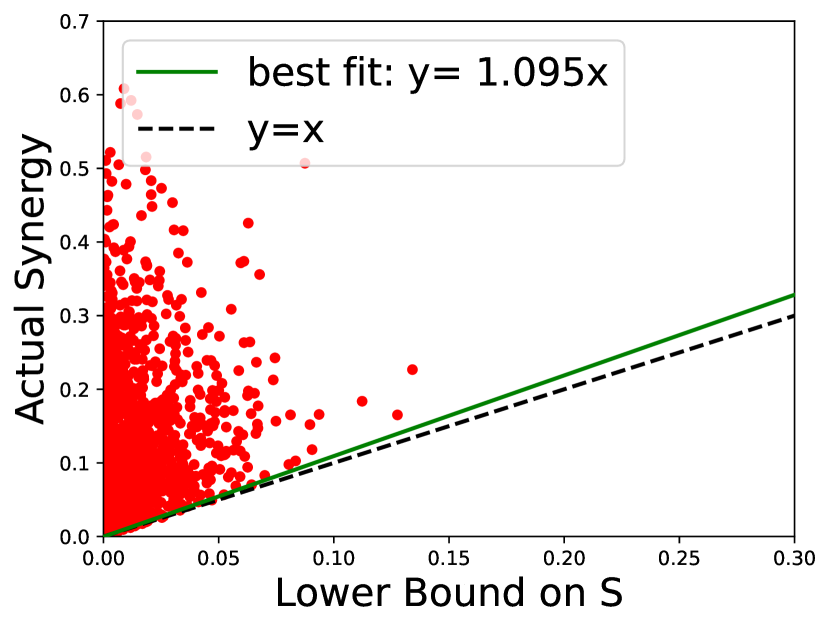
(a) $S$ vs $\underline{S}_{\textrm{agree}}$

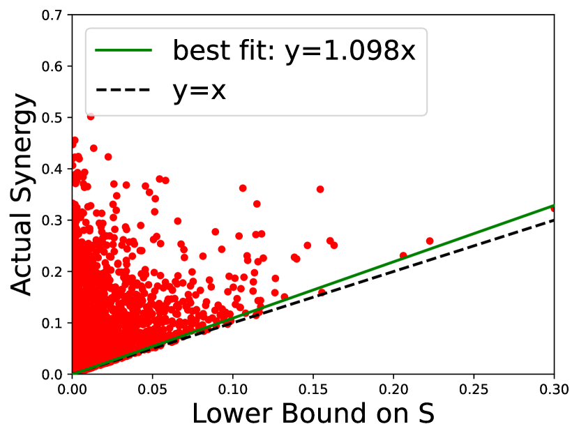
(b) $S$ vs $\underline{S}_{\textrm{disagree}}$

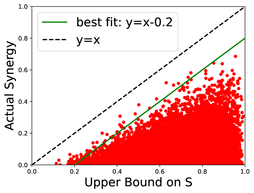
(c) $S$ vs $\overline{S}$

Figure 7: Plots of actual synergy against our estimated (a) lower bound on disagreement synergy, (b) lower bound on agreement synergy, and (c) upper bound. The bounds closely track true synergy, which we show via three lines of best fit that almost exactly track true synergy: $y=1.095x$, $y=1.098x$, and $y=x-0.2$.

Results: We calculated the lower bound via redundancy, lower bound via disagreement, and upper bound of all distributions and plotted them with actual synergy value (Figure 7). We define a distribution to be on the boundary if its lower/upper bound is within $10\%$ difference from its actual synergy value. We conducted the least mean-square-error fitting on these distributions close to the boundary. We plot actual synergy against $\underline{S}_{\textrm{agree}}$ in Figure 7 (left), and find that it again tracks a lower bound of synergy. In fact, we can do better and fit a linear trend $y=1.095x$ on the distributions along the margin (RMSE $=0.0013$).

We also plot actual synergy against computed $\underline{S}_{\textrm{disagree}}$ in Figure 7 (middle). As expected, the lower bound closely tracks actual synergy. Similarly, we can again fit a linear model on the points along the boundary, obtaining $y=1.098x$ with a RMSE of $0.0075$ (see this line in Figure 7 (middle)).

Finally, we plot actual synergy against estimated $\overline{S}$ in Figure 7 (right). Again, we find that the upper bound consistently tracks the highest attainable synergy - we can fit a single constant $y=x-0.2$ to obtain an RMSE of $0.0022$ (see this line in Figure 7 (right)). This implies that our bound enables both accurate comparative analysis of relative synergy across different datasets, and precise estimation of absolute synergy.

Real-world datasets: We also use the large collection of real-world datasets in MultiBench [61]: (1) MOSI: video-based sentiment analysis [103], (2) MOSEI: video-based sentiment and emotion analysis [106], (3) MUStARD: video-based sarcasm detection [14], (5) MIMIC: mortality and disease prediction from tabular patient data and medical sensors [53], and (6) ENRICO: classification of mobile user interfaces and screenshots [58]. While the previous bitwise datasets with small and discrete support yield exact lower and upper bounds, this new setting with high-dimensional continuous modalities requires the approximation of disagreement and information-theoretic quantities: we train unimodal neural network classifiers $\hat{f}_{\theta}(y|x_{1})$ and $\hat{f}_{\theta}(y|x_{2})$ to estimate disagreement, and we cluster representations of $X_{i}$ to approximate the continuous modalities by discrete distributions with finite support to compute lower and upper bounds.

Implementation details: We first apply PCA to reduce the dimension of multimodal data. For the test split, we use unsupervised clustering to generate $20$ clusters. We obtain a clustered version of the original dataset $\mathcal{D}=\{(x_{1},x_{2},y)\}$ as $\mathcal{D}_{\text{cluster}}=\{(c_{1},c_{2},y)\}$ where $c_{i}\in\{1,\dots,20\}$ is the ID of the cluster that $x_{i}$ belongs to. In our experiments, where $\mathcal{Y}$ is typically a classification task, we set the unimodal classifiers $f_{1}=\hat{p}(y|x_{1})$ and $f_{2}=\hat{p}(y|x_{2})$ as the Bayes optimal classifiers for multiclass classification tasks.

For classification, $\mathcal{Y}$ is the set of $k$-dimensional 1-hot vectors. Given two logits $\hat{y}_{1},\hat{y}_{2}$ obtained from $x_{1},x_{2}$ respectively, define $d(\hat{y}_{1},\hat{y}_{2})=\left(\hat{y}_{1}-\hat{y}_{2}\right)^{2}$. We have that $c_{d}=1$, and $\epsilon_{1}=|L(f_{1})-L(f_{1}^{*})|^{2}=0$ and $\epsilon_{2}=|L(f_{2})-L(f_{2}^{*})|^{2}=0$ for well-trained neural network unimodal classifiers $f_{1}$ and $f_{2}$ for Theorem 2. For datasets with $3$ modalities, we perform the experiments separately for each of the $3$ modality pairs, before taking an average over the $3$ modality pairs. Extending the definitions of redundancy, uniqueness, and synergy, as well as our derived bounds on synergy for 3 or more modalities is an important open question for future work.

B.2 Relationships between agreement, disagreement, and interactions

1. The relationship between redundancy and synergy: We give some example distributions to analyze when the lower bound based on redundancy $\underline{S}_{\textrm{agree}}$ is high or low. The bound is high for distributions where $X_{1}$ and $X_{2}$ are independent, but $Y=1$ sets $X_{1}\neq X_{2}$ to increase their dependence (i.e., agreement XOR distribution in Table 2(b)). Since $X_{1}$ and $X_{2}$ are independent but become dependent given $Y$, $I(X_{1};X_{2};Y)$ is negative, and the bound is tight $\underline{S}_{\textrm{agree}}=1\leq 1=S$. Visual Question Answering 2.0 [37] falls under this category, with $S=4.92,R=0.79$, where the image and question are independent (some questions like ‘what is the color of the object’ or ‘how many people are there’ can be asked for many images), but the answer connects the two modalities, resulting in dependence given the label. As expected, the estimated lower bound for agreement synergy: $\underline{S}_{\textrm{agree}}=4.03\leq 4.92=S$.

Conversely, the bound is low for Table 2(d) with the probability mass distributed uniformly only when $y=x_{1}=x_{2}$ and $0$ elsewhere. As a result, $X_{1}$ is always equal to $X_{2}$ (perfect dependence), and yet $Y$ perfectly explains away the dependence between $X_{1}$ and $X_{2}$ so $I(X_{1};X_{2}|Y)=0$: $\underline{S}_{\textrm{agree}}=0\leq 0=S$. Note that this is an example of perfect redundancy and zero synergy - for an example with synergy, refer back to disagreement XOR in Table 2(a) - due to disagreement there is non-zero $I(X_{1};X_{2})$ but the label explains some of the relationships between $X_{1}$ and $X_{2}$ so $I(X_{1};X_{2}|Y)<I(X_{1};X_{2})$: $\underline{S}_{\textrm{agree}}=-0.3\leq 1=S$. A real-world example is multimodal sentiment analysis from text, video, and audio of monologue videos on MOSEI, $R=0.26$ and $S=0.04$, and as expected the lower bound is small $\underline{S}_{\textrm{agree}}=0.01\leq 0.04=S$.

2. The relationship between disagreement and synergy: To give an intuition of the relationship between disagreement, uniqueness, and synergy, we use one illustrative example shown in Table 2(a), which we call disagreement XOR. We observe that there is maximum disagreement between marginals $p(y|x_{1})$ and $p(y|x_{2})$: the likelihood for $y$ is high when $y$ is the same bit as $x_{1}$, but reversed for $x_{2}$. Given both $x_{1}$ and $x_{2}$: $y$ seems to take a ‘disagreement’ XOR of the individual marginals, i.e. $p(y|x_{1},x_{2})=p(y|x_{1})\ \textrm{XOR}\ p(y|x_{2})$, which indicates synergy (note that an exact XOR would imply perfect agreement and high synergy). The actual disagreement is $0.15$, synergy is $0.16$, and uniqueness is $0.02$, indicating a very strong lower bound $\underline{S}_{\textrm{disagree}}=0.13\leq 0.16=S$. A real-world equivalent dataset is MUStARD for sarcasm detection from video, audio, and text [14], where the presence of sarcasm is often due to a contradiction between what is expressed in language and speech, so disagreement $\alpha=0.12$ is the highest out of all the video datasets, giving a lower bound $\underline{S}_{\textrm{disagree}}=0.11\leq 0.44=S$.

On the contrary, the lower bound is low when all disagreement is explained by uniqueness (e.g., $y=x_{1}$, Table 2(c)), which results in $\underline{S}_{\textrm{disagree}}=0\leq 0=S$ ($\alpha$ and $U$ cancel each other out). A real-world equivalent is MIMIC involving mortality and disease prediction from tabular patient data and time-series medical sensors [53]. Disagreement is high $\alpha=0.13$ due to unique information $U_{1}=0.25$, so the lower bound informs us about the lack of synergy $\underline{S}_{\textrm{disagree}}=-0.12\leq 0.02=S$.

Finally, the lower bound is loose when there is synergy without disagreement, such as agreement XOR ($y=x_{1}\textrm{ XOR }x_{2}$, Table 2(b)) where the marginals $p(y|x_{i})$ are both uniform, but there is full synergy: $\underline{S}_{\textrm{disagree}}=0\leq 1=S$. Real-world datasets which fall into agreement synergy include UR-FUNNY where there is low disagreement in predicting humor $\alpha=0.03$, and relatively high synergy $S=0.18$, which results in a loose lower bound $\underline{S}_{\textrm{disagree}}=0.01\leq 0.18=S$.

Figure 8: Comparing the qualities of the bounds when there is agreement and disagreement synergy. During agreement synergy, $\underline{S}_{\textrm{agree}}$ is tight, $\underline{S}_{\textrm{disagree}}$ is loose, and $\overline{S}$ is tight. For disagreement synergy, $\underline{S}_{\textrm{agree}}$ is loose, $\underline{S}_{\textrm{disagree}}$ is tight, and $\overline{S}$ is loose with respect to true $S$.

3. On upper bounds for synergy: We also run experiments to obtain estimated upper bounds on synthetic and MultiBench datasets. The quality of the upper bound shows some intriguing relationships with that of lower bounds. For distributions with perfect agreement synergy such as $y=x_{1}\textrm{ XOR }x_{2}$ (Table 2(b)), $\overline{S}=1\geq 1=S$ is really close to true synergy, $\underline{S}_{\textrm{agree}}=1\leq 1=S$ is also tight, but $\underline{S}_{\textrm{disagree}}=0\leq 1=S$ is loose. For distributions with disagreement synergy (Table 2(a)), $\overline{S}=0.52\geq 0.13=S$ far exceeds actual synergy, $\underline{S}_{\textrm{agree}}=-0.3\leq 1=S$ is much lower than actual synergy, but $\underline{S}_{\textrm{disagree}}=0.13\leq 0.16=S$ is tight (see relationships in Figure 8).

Finally, while some upper bounds (e.g., MUStARD, MIMIC) are close to true $S$, some of the other examples in Table 1 show bounds that are quite weak. This could be because (i) there indeed exists high synergy distributions that match $\mathcal{D}_{i}$ and $\mathcal{D}_{M}$, but these are rare in the real world, or (ii) our approximation used in Theorem 4 is mathematically loose. We leave these as open directions for future work.

Table 5: We show the full list of computed lower and upper bounds on $S$ without labeled multimodal data and compare them to the true $S$ assuming knowledge of the full joint distribution $p$: the bounds track $S$ well on MUStARD and MIMIC, and also show general trends on the other datasets except ENRICO where estimating synergy is difficult. V = video, T = text, A = audio modalities.

	MOSEI${}_{\text{V+T}}$	MOSEI${}_{\text{V+A}}$	MOSEI${}_{\text{A+T}}$	UR-FUNNY${}_{\text{V+T}}$	UR-FUNNY${}_{\text{V+A}}$	UR-FUNNY${}_{\text{A+T}}$
$\overline{S}$	$0.96$	$0.98$	$0.97$	$0.96$	$0.96$	$0.99$
$S$	$0.04$	$0.03$	$0.03$	$0.21$	$0.24$	$0.08$
$\underline{S}_{\textrm{agree}}$	$0.01$	$0.0$	$0.0$	$0.0$	$0.0$	$0.0$
$\underline{S}_{\textrm{disagree}}$	$0.01$	$0.01$	$0.0$	$0.0$	$0.0$	$0.01$

	MOSI${}_{\text{V,T}}$	MOSI${}_{\text{V,A}}$	MOSI${}_{\text{A,T}}$	MUStARD${}_{\text{V,T}}$	MUStARD${}_{\text{V,A}}$	MUStARD${}_{\text{A,T}}$	MIMIC	ENRICO
$\overline{S}$	$0.92$	$0.92$	$0.93$	$0.79$	$0.78$	$0.79$	$0.41$	$2.09$
$S$	$0.31$	$0.28$	$0.14$	$0.49$	$0.31$	$0.51$	$0.02$	$1.02$
$\underline{S}_{\textrm{agree}}$	$0.01$	$0.01$	$0.0$	$0.04$	$0.01$	$0.06$	$0.0$	$0.01$
$\underline{S}_{\textrm{disagree}}$	$0.03$	$0.03$	$0.02$	$0.07$	$0.06$	$0.11$	$-0.12$	$-0.55$

Appendix C Application 1: Estimating multimodal performance for fusion

Formally, we estimate performance via a combination of Feder and Merhav [29] and Fano’s inequality [27] together yield tight bounds of performance as a function of total information $I_{p}(\{X_{1},X_{2}\};Y)$. We restate Theorem 5 from the main text:

Theorem 9.

Let $P_{\textrm{acc}}(f_{M}^{*})=\mathbb{E}_{p}\left[\mathbf{1}\left[f_{M}^{*}(x_{1},x_{2})=y\right]\right]$ denote the accuracy of the Bayes’ optimal multimodal model $f_{M}^{*}$ (i.e., $P_{\textrm{acc}}(f_{M}^{*})\geq P_{\textrm{acc}}(f^{\prime}_{M})$ for all $f^{\prime}_{M}\in\mathcal{F}_{M}$). We have that

$$2^{I_{p}(\{X_{1},X_{2}\};Y)-H(Y)}\leq P_{\textrm{acc}}(f_{M}^{*})\leq\frac{I_{p}(\{X_{1},X_{2}\};Y)+1}{\log|\mathcal{Y}|},$$ (54)

where we can plug in $R+U_{1},U_{2}+\underline{S}\leq I_{p}(\{X_{1},X_{2}\};Y)\leq R+U_{1},U_{2}+\overline{S}$ to obtain lower $\underline{P}_{\textrm{acc}}(f_{M}^{*})$ and upper $\overline{P}_{\textrm{acc}}(f_{M}^{*})$ bounds on optimal multimodal performance.

Proof.

We use the bound from Feder and Merhav [29], where we define the Bayes’ optimal classifier $f_{M}^{*}$ is the one where given $x_{1},x_{2}$ outputs $y$ such that $p(Y=y|x_{1},x_{2})$ is maximized over all $y\in\mathcal{Y}$. The probability that this classifier succeeds is $\max_{y}p(Y=y|x_{1},x_{2})$, which is $2^{-H_{\infty}(Y|X_{1}=x_{1},X_{2}=x_{2}))}$ where $-H_{\infty}(Y|X_{1},X_{2})$ is the min-entropy of the random variable $Y$ conditioned on $X_{1},X_{2}$. Over all inputs $(x_{1},x_{2})$, the probability of accuracy is

$$P_{\textrm{acc}}(f_{M}^{*}) =\mathbb{E}_{x_{1},x_{2}}\left[2^{-H_{\infty}(Y|X_{1}=x_{1},X_{2}=x_{2}))}\right]\geq 2^{-\mathbb{E}_{x_{1},x_{2}}\left[H_{\infty}(Y|X_{1}=x_{1},X_{2}=x_{2}))\right]}$$ (55)

$$\geq 2^{-\mathbb{E}_{x_{1},x_{2}}\left[H_{p}(Y|X_{1}=x_{1},X_{2}=x_{2}))\right]}\geq 2^{-H_{p}(Y|X_{1},X_{2})}=2^{I_{p}(\{X_{1},X_{2}\};Y)-H(Y)}.$$ (56)

The upper bound is based on Fano’s inequality [27]. Starting with $H_{p}(Y|X_{1},X_{2})\leq H(P_{\textrm{err}})+P_{\textrm{err}}(\log|\mathcal{Y}|-1)$ and assuming that $Y$ is uniform over $|\mathcal{Y}|$, we rearrange the inequality to obtain

$$P_{\textrm{acc}}(f_{M}^{*})\leq\frac{H(Y)-H_{p}(Y|X_{1},X_{2})+\log 2}{\log|\mathcal{Y}|}=\frac{I_{p}(\{X_{1},X_{2}\};Y)+1}{\log|\mathcal{Y}|}.$$ (57)

∎

Finally, we summarize estimated multimodal performance as the average between estimated lower and upper bounds on performance: $\hat{P}_{M}=(\underline{P}_{\textrm{acc}}(f_{M}^{*})+\overline{P}_{\textrm{acc}}(f_{M}^{*}))/2$.

Table 6: Full list of best unimodal performance $P_{\textrm{acc}}(f_{i})$, best simple fusion $P_{\textrm{acc}}(f_{M\textrm{simple}})$, and best complex fusion $P_{\textrm{acc}}(f_{M\textrm{complex}})$ as obtained from the most recent state-of-the-art models. We also include our estimated bounds $(\underline{P}_{\textrm{acc}}(f_{M}^{*}),\overline{P}_{\textrm{acc}}(f_{M}^{*}))$ on optimal multimodal performance.

	MOSEI	UR-FUNNY	MOSI	MUStARD	MIMIC	ENRICO
$\overline{P}_{\textrm{acc}}(f_{M}^{*})$	$1.07$	$1.21$	$1.29$	$1.63$	$1.27$	$0.88$
$P_{\textrm{acc}}(f_{M\textrm{complex}})$	$0.88$ [49]	$0.77$ [41]	$0.86$ [49]	$0.79$ [41]	$0.92$ [61]	$0.51$ [61]
$P_{\textrm{acc}}(f_{M\textrm{simple}})$	$0.85$ [77]	$0.76$ [41]	$0.84$ [77]	$0.74$ [75]	$0.92$ [61]	$0.49$ [61]
$P_{\textrm{acc}}(f_{i})$	$0.82$ [22]	$0.74$ [41]	$0.83$ [99]	$0.74$ [41]	$0.92$ [61]	$0.47$ [61]
$\underline{P}_{\textrm{acc}}(f_{M}^{*})$	$0.52$	$0.58$	$0.62$	$0.78$	$0.76$	$0.48$

Unimodal and multimodal performance: Table 6 summarizes all final performance results for each dataset, spanning unimodal models and simple or complex multimodal fusion paradigms, where each type of model is represented by the most recent state-of-the-art method found in the literature.

Appendix D Application 2: Self-supervised multimodal learning via disagreement

D.1 Training procedure

We continuously pretrain MERLOT Reserve Base on the datasets before finetuning. The continuous pretraining procedure is similar to Contrastive Span Training, with the difference that we add extra loss terms that correspond to modality disagreement. The pretraining procedure of MERLOT Reserve minimizes a sum of 3 component losses,

$$\mathcal{L}=\mathcal{L_{\text{text}}}+\mathcal{L_{\text{audio}}}+\mathcal{L_{\text{frame}}}$$

where each of the component losses is a contrastive objective. Each of the objectives aims to match an independent encoding of masked tokens of the corresponding modality with the output of a Joint Encoder, which takes as input the other modalities and, possibly, unmasked tokens of the target modality.

We modify the procedure by adding disagreement losses between modalities to the objective. This is done by replacing the tokens of a modality with padding tokens before passing them to the Joint Encoder, and then calculating the disagreement between representations obtained when replacing different modalities. For example, $\mathcal{L}_{\text{frame}}$ uses a representation of video frames found by passing audio and text into the Joint Encoder. Excluding one of the modalities and passing the other one into the Encoder separately leads to two different representations, $\mathbb{\hat{f}_{t}}$ for prediction using only text and $\mathbb{\hat{f}_{a}}$ for prediction using only audio. The distance between the representations is added to the loss. Thus, the modified component loss is

$$\mathcal{L}_{\text{disagreement, frame}}=\mathcal{L}_{\text{frame}}+d_{\lambda_{\text{text, audio}}}(\mathbb{\hat{f}_{t}},\mathbb{\hat{f}_{a}})$$

where $d_{\lambda_{\text{text, audio}}}(\mathbb{x},\mathbb{y})=\max(0,d(\mathbb{x},\mathbb{y})-\lambda_{\text{text, audio}})$, and $d(\mathbb{x},\mathbb{y})$ is the cosine difference:

$$d(\mathbb{x},\mathbb{y})=1-\frac{\mathbb{x}\cdot\mathbb{y}}{|\mathbb{x}||\mathbb{y}|}$$

Similarly, we modify the other component losses by removing one modality at a time, and obtain the new training objective

$$\mathcal{L}_{\text{disagreement}}=\mathcal{L_{\text{disagreement, text}}}+\mathcal{L_{\text{disagreement, audio}}}+\mathcal{L_{\text{disagreement, frame}}}$$

D.2 Training details

We continuously pretrain and then finetune a pretrained MERLOT Reserve Base model on the datasets with a batch size of 8. During pretraining, we train the model for 960 steps with a learning rate of 0.0001, and no warm-up steps, and use the defaults for other hyperparameters. For every dataset, we fix two of $\{\lambda_{\text{text, audio}},\lambda_{\text{vision, audio}},\lambda_{\text{text, vision}}\}$ to be $+\infty$ and change the third one, which characterizes the most meaningful disagreement. This allows us to reduce the number of masked modalities required from 3 to 2 and thus reduce the memory overhead of the method. For Social-IQ, we set $\lambda_{\text{text, vision}}$ to be 0. For UR-FUNNY, we set $\lambda_{\text{text, vision}}$ to be 0.5. For MUStARD, we set $\lambda_{\text{vision, audio}}$ to be 0. All training is done on TPU v2-8 accelerators, with continuous pretraining taking 30 minutes and using up to $9$GB of memory.

D.3 Dataset level analysis

We visualize the impact of pairwise modality disagreement on model performance by fixing two modalities $M_{1},M_{2}$ and a threshold $t$, and setting the modality pair-specific disagreement slack terms $\lambda$ according to the rule

$$\lambda_{a,b}=\begin{cases}t,&a=M_{1},b=M_{2}\\ +\infty,&\text{else}\end{cases}$$

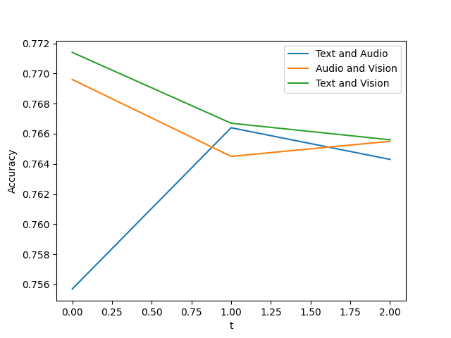
Figure 9: Impact of modality disagreement on model performance. Lower $t$ means we train with higher disagreement between modalities: we find that disagreement between text and vision, as well as audio and vision, are more helpful during self-supervised masking with performance improvements, whereas disagreement between text and audio is less suitable and can even hurt performance.

This allows us to isolate $d_{\lambda_{M_{1},M_{2}}}$ while ensuring that the other disagreement loss terms are 0. We also modify the algorithm to subtract $d_{\lambda_{M_{1},M_{2}}}$ from the loss rather than adding it (see Section D.5). By decreasing $t$, we encourage higher disagreement between the target modalities. In Figure 9, we plot the relationship between model accuracy and $t$ for the MUStARD dataset to visualize how pairwise disagreement between modalities impacts model performance.

D.4 Datapoint level analysis

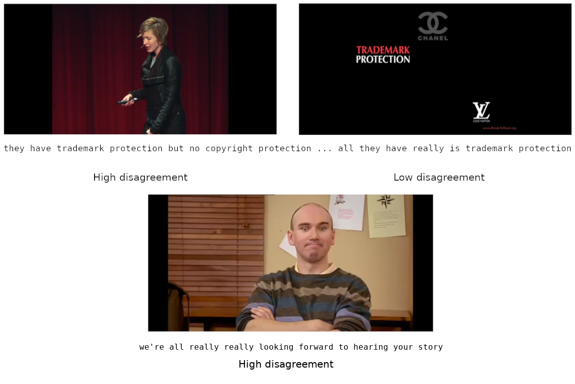
Figure 10: Examples of disagreement due to uniqueness (up) and synergy (down)

After continuously pretraining the model, we fix a pair of modalities (text and video) and find the disagreement in these modalities for each datapoint. We show examples of disagreement due to uniqueness and synergy in Figure 10. The first example shows a speaker using descriptive slides, leading to less unique information being present in the text and higher agreement between modalities. In the second example, the facial expression of the person shown does not match the text being spoken, indicating sarcasm and leading to disagreement synergy.

D.5 Alternative training procedure

We also explore an alternative training procedure, which involves subtracting the disagreements $d_{\lambda_{a,b}}$ from the loss rather than adding them. This achieves the opposite effect of pushing modalities further away from each other if they disagree significantly. The reasoning behind this is that in some settings, such as sarcasm prediction in MUStARD, we expect modalities not just to disagree, but to store contradicting information, and disagreement between them should be encouraged. However, we find that the results obtained using this method are not as good as the ones obtained using the procedure outlined in Section D.1.

References

- Aghajanyan et al. [2023] Armen Aghajanyan, Lili Yu, Alexis Conneau, Wei-Ning Hsu, Karen Hambardzumyan, Susan Zhang, Stephen Roller, Naman Goyal, Omer Levy, and Luke Zettlemoyer. Scaling laws for generative mixed-modal language models. arXiv preprint arXiv:2301.03728, 2023.
- Antol et al. [2015] Stanislaw Antol, Aishwarya Agrawal, Jiasen Lu, Margaret Mitchell, Dhruv Batra, C Lawrence Zitnick, and Devi Parikh. Vqa: Visual question answering. In Proceedings of the IEEE international conference on computer vision, pages 2425–2433, 2015.
- ApS [2022] MOSEK ApS. MOSEK Optimizer API for Python 10.0.34, 2022. URL https://docs.mosek.com/latest/pythonapi/index.html.
- Baek et al. [2022] Christina Baek, Yiding Jiang, Aditi Raghunathan, and J Zico Kolter. Agreement-on-the-line: Predicting the performance of neural networks under distribution shift. Advances in Neural Information Processing Systems, 35:19274–19289, 2022.
- Balcan et al. [2004] Maria-Florina Balcan, Avrim Blum, and Ke Yang. Co-training and expansion: Towards bridging theory and practice. Advances in neural information processing systems, 17, 2004.
- Baltrušaitis et al. [2018] Tadas Baltrušaitis, Chaitanya Ahuja, and Louis-Philippe Morency. Multimodal machine learning: A survey and taxonomy. IEEE transactions on pattern analysis and machine intelligence, 41(2):423–443, 2018.
- Baron and Kenny [1986] Reuben M Baron and David A Kenny. The moderator–mediator variable distinction in social psychological research: Conceptual, strategic, and statistical considerations. Journal of personality and social psychology, 51(6):1173, 1986.
- Bell [2003] Anthony J Bell. The co-information lattice. In Proceedings of the fifth international workshop on independent component analysis and blind signal separation: ICA, volume 2003, 2003.
- Bengio and Bourlard [2005] Samy Bengio and Hervé Bourlard. Machine learning for multimodal interaction. Springer, 2005.
- Bertschinger et al. [2014] Nils Bertschinger, Johannes Rauh, Eckehard Olbrich, Jürgen Jost, and Nihat Ay. Quantifying unique information. Entropy, 2014.
- Birhane et al. [2021] Abeba Birhane, Vinay Uday Prabhu, and Emmanuel Kahembwe. Multimodal datasets: misogyny, pornography, and malignant stereotypes. arXiv preprint arXiv:2110.01963, 2021.
- Blum and Mitchell [1998] Avrim Blum and Tom Mitchell. Combining labeled and unlabeled data with co-training. In Proceedings of the eleventh annual conference on Computational learning theory, pages 92–100, 1998.
- Bolukbasi et al. [2016] Tolga Bolukbasi, Kai-Wei Chang, James Y Zou, Venkatesh Saligrama, and Adam T Kalai. Man is to computer programmer as woman is to homemaker? debiasing word embeddings. Advances in neural information processing systems, 29, 2016.
- Castro et al. [2019] Santiago Castro, Devamanyu Hazarika, Verónica Pérez-Rosas, Roger Zimmermann, Rada Mihalcea, and Soujanya Poria. Towards multimodal sarcasm detection (an _obviously_ perfect paper). In ACL, pages 4619–4629, 2019.
- Christoudias et al. [2008] C Mario Christoudias, Raquel Urtasun, and Trevor Darrell. Multi-view learning in the presence of view disagreement. In Proceedings of the Twenty-Fourth Conference on Uncertainty in Artificial Intelligence, 2008.
- Cicalese and Vaccaro [2002] Ferdinando Cicalese and Ugo Vaccaro. Supermodularity and subadditivity properties of the entropy on the majorization lattice. IEEE Transactions on Information Theory, 48(4):933–938, 2002.
- Cicalese et al. [2017] Ferdinando Cicalese, Luisa Gargano, and Ugo Vaccaro. How to find a joint probability distribution of minimum entropy (almost) given the marginals. In 2017 IEEE International Symposium on Information Theory (ISIT), pages 2173–2177. IEEE, 2017.
- Colenbier et al. [2020] Nigel Colenbier, Frederik Van de Steen, Lucina Q Uddin, Russell A Poldrack, Vince D Calhoun, and Daniele Marinazzo. Disambiguating the role of blood flow and global signal with partial information decomposition. Neuroimage, 213:116699, 2020.
- Compton [2022] Spencer Compton. A tighter approximation guarantee for greedy minimum entropy coupling. In 2022 IEEE International Symposium on Information Theory (ISIT), pages 168–173. IEEE, 2022.
- Compton et al. [2023] Spencer Compton, Dmitriy Katz, Benjamin Qi, Kristjan Greenewald, and Murat Kocaoglu. Minimum-entropy coupling approximation guarantees beyond the majorization barrier. In International Conference on Artificial Intelligence and Statistics, pages 10445–10469. PMLR, 2023.
- Cortes et al. [2019] Corinna Cortes, Giulia DeSalvo, Mehryar Mohri, Ningshan Zhang, and Claudio Gentile. Active learning with disagreement graphs. In International Conference on Machine Learning, pages 1379–1387. PMLR, 2019.
- Delbrouck et al. [2020] Jean-Benoit Delbrouck, Noé Tits, Mathilde Brousmiche, and Stéphane Dupont. A transformer-based joint-encoding for emotion recognition and sentiment analysis. In Second Grand-Challenge and Workshop on Multimodal Language (Challenge-HML), pages 1–7, Seattle, USA, July 2020. Association for Computational Linguistics. doi: 10.18653/v1/2020.challengehml-1.1. URL https://aclanthology.org/2020.challengehml-1.1.
- Deng et al. [2009] Jia Deng, Wei Dong, Richard Socher, Li-Jia Li, Kai Li, and Li Fei-Fei. Imagenet: A large-scale hierarchical image database. In 2009 IEEE conference on computer vision and pattern recognition, pages 248–255. Ieee, 2009.
- Ding et al. [2022] Daisy Yi Ding, Shuangning Li, Balasubramanian Narasimhan, and Robert Tibshirani. Cooperative learning for multiview analysis. Proceedings of the National Academy of Sciences, 119(38):e2202113119, 2022.
- Domahidi et al. [2013] Alexander Domahidi, Eric Chu, and Stephen Boyd. Ecos: An socp solver for embedded systems. In 2013 European Control Conference (ECC), pages 3071–3076. IEEE, 2013.
- Even et al. [1975] Shimon Even, Alon Itai, and Adi Shamir. On the complexity of time table and multi-commodity flow problems. In 16th annual symposium on foundations of computer science (sfcs 1975), pages 184–193. IEEE, 1975.
- Fano [1968] Robert M Fano. Transmission of information: a statistical theory of communications. Mit Press, 1968.
- Farquhar et al. [2005] Jason Farquhar, David Hardoon, Hongying Meng, John Shawe-Taylor, and Sandor Szedmak. Two view learning: Svm-2k, theory and practice. NeurIPS, 18, 2005.
- Feder and Merhav [1994] Meir Feder and Neri Merhav. Relations between entropy and error probability. IEEE Transactions on Information theory, 40(1):259–266, 1994.
- Flecker et al. [2011] Benjamin Flecker, Wesley Alford, John M Beggs, Paul L Williams, and Randall D Beer. Partial information decomposition as a spatiotemporal filter. Chaos: An Interdisciplinary Journal of Nonlinear Science, 2011.
- Friedman and Popescu [2008] Jerome H Friedman and Bogdan E Popescu. Predictive learning via rule ensembles. The annals of applied statistics, 2(3):916–954, 2008.
- Fukui et al. [2016] Akira Fukui, Dong Huk Park, Daylen Yang, Anna Rohrbach, Trevor Darrell, and Marcus Rohrbach. Multimodal compact bilinear pooling for visual question answering and visual grounding. In Conference on Empirical Methods in Natural Language Processing. ACL, 2016.
- Garner [1962] Wendell R Garner. Uncertainty and structure as psychological concepts. 1962.
- Gawne and Richmond [1993] Timothy J Gawne and Barry J Richmond. How independent are the messages carried by adjacent inferior temporal cortical neurons? Journal of Neuroscience, 13(7):2758–2771, 1993.
- Ghassami and Kiyavash [2017] AmirEmad Ghassami and Negar Kiyavash. Interaction information for causal inference: The case of directed triangle. In 2017 IEEE International Symposium on Information Theory (ISIT), pages 1326–1330. IEEE, 2017.
- Globerson and Jaakkola [2007] Amir Globerson and Tommi Jaakkola. Approximate inference using conditional entropy decompositions. In Artificial Intelligence and Statistics, pages 131–138. PMLR, 2007.
- Goyal et al. [2017] Yash Goyal, Tejas Khot, Douglas Summers-Stay, Dhruv Batra, and Devi Parikh. Making the v in vqa matter: Elevating the role of image understanding in visual question answering. In Proceedings of the IEEE Conference on Computer Vision and Pattern Recognition, pages 6904–6913, 2017.
- Griffith and Koch [2014] Virgil Griffith and Christof Koch. Quantifying synergistic mutual information. In Guided self-organization: inception, pages 159–190. Springer, 2014.
- Hanneke et al. [2014] Steve Hanneke et al. Theory of disagreement-based active learning. Foundations and Trends® in Machine Learning, 7(2-3):131–309, 2014.
- Hasan et al. [2019] Md Kamrul Hasan, Wasifur Rahman, AmirAli Bagher Zadeh, Jianyuan Zhong, Md Iftekhar Tanveer, Louis-Philippe Morency, and Mohammed Ehsan Hoque. Ur-funny: A multimodal language dataset for understanding humor. In Proceedings of the 2019 Conference on Empirical Methods in Natural Language Processing and the 9th International Joint Conference on Natural Language Processing (EMNLP-IJCNLP), pages 2046–2056, 2019.
- Hasan et al. [2021] Md Kamrul Hasan, Sangwu Lee, Wasifur Rahman, Amir Zadeh, Rada Mihalcea, Louis-Philippe Morency, and Ehsan Hoque. Humor knowledge enriched transformer for understanding multimodal humor. Proceedings of the AAAI Conference on Artificial Intelligence, 35(14):12972–12980, May 2021. doi: 10.1609/aaai.v35i14.17534. URL https://ojs.aaai.org/index.php/AAAI/article/view/17534.
- Hastie and Tibshirani [1987] Trevor Hastie and Robert Tibshirani. Generalized additive models: some applications. Journal of the American Statistical Association, 1987.
- Hessel and Lee [2020] Jack Hessel and Lillian Lee. Does my multimodal model learn cross-modal interactions? it’s harder to tell than you might think! In EMNLP, 2020.
- Hessel et al. [2022] Jack Hessel, Ana Marasović, Jena D Hwang, Lillian Lee, Jeff Da, Rowan Zellers, Robert Mankoff, and Yejin Choi. Do androids laugh at electric sheep? humor" understanding" benchmarks from the new yorker caption contest. arXiv preprint arXiv:2209.06293, 2022.
- Hornik et al. [1989] Kurt Hornik, Maxwell Stinchcombe, and Halbert White. Multilayer feedforward networks are universal approximators. Neural networks, 2(5):359–366, 1989.
- Hou et al. [2019] Ming Hou, Jiajia Tang, Jianhai Zhang, Wanzeng Kong, and Qibin Zhao. Deep multimodal multilinear fusion with high-order polynomial pooling. Advances in Neural Information Processing Systems, 32:12136–12145, 2019.
- Hsu et al. [2018] Tzu-Ming Harry Hsu, Wei-Hung Weng, Willie Boag, Matthew McDermott, and Peter Szolovits. Unsupervised multimodal representation learning across medical images and reports. arXiv preprint arXiv:1811.08615, 2018.
- Hu et al. [2019] Di Hu, Feiping Nie, and Xuelong Li. Deep multimodal clustering for unsupervised audiovisual learning. In Proceedings of the IEEE/CVF Conference on Computer Vision and Pattern Recognition, pages 9248–9257, 2019.
- Hu et al. [2022] Guimin Hu, Ting-En Lin, Yi Zhao, Guangming Lu, Yuchuan Wu, and Yongbin Li. UniMSE: Towards unified multimodal sentiment analysis and emotion recognition. In Proceedings of the 2022 Conference on Empirical Methods in Natural Language Processing, pages 7837–7851, Abu Dhabi, United Arab Emirates, December 2022. Association for Computational Linguistics. URL https://aclanthology.org/2022.emnlp-main.534.
- James et al. [2018] Ryan G James, Jeffrey Emenheiser, and James P Crutchfield. Unique information and secret key agreement. Entropy, 21(1):12, 2018.
- Jayakumar et al. [2020] Siddhant M. Jayakumar, Wojciech M. Czarnecki, Jacob Menick, Jonathan Schwarz, Jack Rae, Simon Osindero, Yee Whye Teh, Tim Harley, and Razvan Pascanu. Multiplicative interactions and where to find them. In International Conference on Learning Representations, 2020.
- Jiang et al. [2022] Yiding Jiang, Vaishnavh Nagarajan, Christina Baek, and J Zico Kolter. Assessing generalization of sgd via disagreement. In International Conference on Learning Representations, 2022.
- Johnson et al. [2016] Alistair EW Johnson, Tom J Pollard, Lu Shen, Li-wei H Lehman, Mengling Feng, Mohammad Ghassemi, Benjamin Moody, Peter Szolovits, Leo Anthony Celi, and Roger G Mark. Mimic-iii, a freely accessible critical care database. Scientific data, 3(1):1–9, 2016.
- Kim et al. [2021] Wonjae Kim, Bokyung Son, and Ildoo Kim. Vilt: Vision-and-language transformer without convolution or region supervision. In International Conference on Machine Learning, pages 5583–5594. PMLR, 2021.
- Kocaoglu et al. [2017] Murat Kocaoglu, Alexandros Dimakis, Sriram Vishwanath, and Babak Hassibi. Entropic causal inference. In Proceedings of the AAAI Conference on Artificial Intelligence, volume 31, 2017.
- Kovačević et al. [2015] Mladen Kovačević, Ivan Stanojević, and Vojin Šenk. On the entropy of couplings. Information and Computation, 242:369–382, 2015.
- Lee et al. [2019] Michelle A Lee, Yuke Zhu, Krishnan Srinivasan, Parth Shah, Silvio Savarese, Li Fei-Fei, Animesh Garg, and Jeannette Bohg. Making sense of vision and touch: Self-supervised learning of multimodal representations for contact-rich tasks. In 2019 International Conference on Robotics and Automation (ICRA), pages 8943–8950. IEEE, 2019.
- Leiva et al. [2020] Luis A Leiva, Asutosh Hota, and Antti Oulasvirta. Enrico: A dataset for topic modeling of mobile ui designs. In 22nd International Conference on Human-Computer Interaction with Mobile Devices and Services, pages 1–4, 2020.
- [59] Paul Pu Liang, Ruslan Salakhutdinov, and Louis-Philippe Morency. Computational modeling of human multimodal language: The mosei dataset and interpretable dynamic fusion.
- Liang et al. [2019] Paul Pu Liang, Zhun Liu, Yao-Hung Hubert Tsai, Qibin Zhao, Ruslan Salakhutdinov, and Louis-Philippe Morency. Learning representations from imperfect time series data via tensor rank regularization. In ACL, 2019.
- Liang et al. [2021a] Paul Pu Liang, Yiwei Lyu, Xiang Fan, Zetian Wu, Yun Cheng, Jason Wu, Leslie Yufan Chen, Peter Wu, Michelle A Lee, Yuke Zhu, et al. Multibench: Multiscale benchmarks for multimodal representation learning. In Thirty-fifth Conference on Neural Information Processing Systems Datasets and Benchmarks Track (Round 1), 2021a.
- Liang et al. [2021b] Paul Pu Liang, Chiyu Wu, Louis-Philippe Morency, and Ruslan Salakhutdinov. Towards understanding and mitigating social biases in language models. In International Conference on Machine Learning, pages 6565–6576. PMLR, 2021b.
- Liang et al. [2021c] Paul Pu Liang, Peter Wu, Liu Ziyin, Louis-Philippe Morency, and Ruslan Salakhutdinov. Cross-modal generalization: Learning in low resource modalities via meta-alignment. In Proceedings of the 29th ACM International Conference on Multimedia, pages 2680–2689, 2021c.
- Liang et al. [2022a] Paul Pu Liang, Yiwei Lyu, Xiang Fan, Shengtong Mo, Dani Yogatama, Louis-Philippe Morency, and Ruslan Salakhutdinov. Highmmt: Towards modality and task generalization for high-modality representation learning. arXiv preprint arXiv:2203.01311, 2022a.
- Liang et al. [2022b] Paul Pu Liang, Amir Zadeh, and Louis-Philippe Morency. Foundations and recent trends in multimodal machine learning: Principles, challenges, and open questions. arXiv preprint arXiv:2209.03430, 2022b.
- Liang et al. [2023a] Paul Pu Liang, Yun Cheng, Xiang Fan, Chun Kai Ling, Suzanne Nie, Richard Chen, Zihao Deng, Faisal Mahmood, Ruslan Salakhutdinov, and Louis-Philippe Morency. Quantifying & modeling feature interactions: An information decomposition framework. arXiv preprint arXiv:2302.12247, 2023a.
- Liang et al. [2023b] Paul Pu Liang, Yiwei Lyu, Gunjan Chhablani, Nihal Jain, Zihao Deng, Xingbo Wang, Louis-Philippe Morency, and Ruslan Salakhutdinov. Multiviz: Towards visualizing and understanding multimodal models. In International Conference on Learning Representations, 2023b. URL https://openreview.net/forum?id=i2_TvOFmEml.
- Liu et al. [2018] Zhun Liu, Ying Shen, Varun Bharadhwaj Lakshminarasimhan, Paul Pu Liang, AmirAli Bagher Zadeh, and Louis-Philippe Morency. Efficient low-rank multimodal fusion with modality-specific factors. In Proceedings of the 56th Annual Meeting of the Association for Computational Linguistics (Volume 1: Long Papers), pages 2247–2256, 2018.
- Maurer and Wolf [1999] Ueli M Maurer and Stefan Wolf. Unconditionally secure key agreement and the intrinsic conditional information. IEEE Transactions on Information Theory, 45(2):499–514, 1999.
- McGill [1954] William McGill. Multivariate information transmission. Transactions of the IRE Professional Group on Information Theory, 4(4):93–111, 1954.
- O’Donoghue et al. [2016] Brendan O’Donoghue, Eric Chu, Neal Parikh, and Stephen Boyd. Conic optimization via operator splitting and homogeneous self-dual embedding. Journal of Optimization Theory and Applications, June 2016.
- Oord et al. [2018] Aaron van den Oord, Yazhe Li, and Oriol Vinyals. Representation learning with contrastive predictive coding. arXiv preprint arXiv:1807.03748, 2018.
- Pathak et al. [2019] Deepak Pathak, Dhiraj Gandhi, and Abhinav Gupta. Self-supervised exploration via disagreement. In International conference on machine learning, pages 5062–5071. PMLR, 2019.
- Pica et al. [2017] Giuseppe Pica, Eugenio Piasini, Houman Safaai, Caroline Runyan, Christopher Harvey, Mathew Diamond, Christoph Kayser, Tommaso Fellin, and Stefano Panzeri. Quantifying how much sensory information in a neural code is relevant for behavior. Advances in Neural Information Processing Systems, 30, 2017.
- Pramanick et al. [2021] Shraman Pramanick, Aniket Basu Roy, and Vishal M. Patel. Multimodal learning using optimal transport for sarcasm and humor detection. 2022 IEEE/CVF Winter Conference on Applications of Computer Vision (WACV), pages 546–556, 2021.
- Radford et al. [2021] Alec Radford, Jong Wook Kim, Chris Hallacy, Aditya Ramesh, Gabriel Goh, Sandhini Agarwal, Girish Sastry, Amanda Askell, Pamela Mishkin, Jack Clark, et al. Learning transferable visual models from natural language supervision. In International Conference on Machine Learning, pages 8748–8763. PMLR, 2021.
- Rahman et al. [2020] Wasifur Rahman, Md Kamrul Hasan, Sangwu Lee, AmirAli Bagher Zadeh, Chengfeng Mao, Louis-Philippe Morency, and Ehsan Hoque. Integrating multimodal information in large pretrained transformers. In Proceedings of the 58th Annual Meeting of the Association for Computational Linguistics, pages 2359–2369, Online, July 2020. Association for Computational Linguistics. doi: 10.18653/v1/2020.acl-main.214. URL https://aclanthology.org/2020.acl-main.214.
- Rossi [2019] Massimiliano Rossi. Greedy additive approximation algorithms for minimum-entropy coupling problem. In 2019 IEEE International Symposium on Information Theory (ISIT), pages 1127–1131. IEEE, 2019.
- Sekar et al. [2020] Ramanan Sekar, Oleh Rybkin, Kostas Daniilidis, Pieter Abbeel, Danijar Hafner, and Deepak Pathak. Planning to explore via self-supervised world models. In International Conference on Machine Learning, pages 8583–8592. PMLR, 2020.
- Shannon [1948] Claude Elwood Shannon. A mathematical theory of communication. The Bell system technical journal, 27(3):379–423, 1948.
- Singh et al. [2022] Amanpreet Singh, Ronghang Hu, Vedanuj Goswami, Guillaume Couairon, Wojciech Galuba, Marcus Rohrbach, and Douwe Kiela. Flava: A foundational language and vision alignment model. In Proceedings of the IEEE/CVF Conference on Computer Vision and Pattern Recognition, pages 15638–15650, 2022.
- Sootla et al. [2017] Sten Sootla, Dirk Oliver Theis, and Raul Vicente. Analyzing information distribution in complex systems. Entropy, 19(12):636, 2017.
- Sorokina et al. [2008] Daria Sorokina, Rich Caruana, Mirek Riedewald, and Daniel Fink. Detecting statistical interactions with additive groves of trees. In Proceedings of the 25th international conference on Machine learning, pages 1000–1007, 2008.
- Sridharan and Kakade [2008] Karthik Sridharan and Sham M Kakade. An information theoretic framework for multi-view learning. In Conference on Learning Theory, 2008.
- Studenỳ and Vejnarová [1998] Milan Studenỳ and Jirina Vejnarová. The multiinformation function as a tool for measuring stochastic dependence. In Learning in graphical models, pages 261–297. Springer, 1998.
- Te Sun [1980] Han Te Sun. Multiple mutual informations and multiple interactions in frequency data. Inf. Control, 46:26–45, 1980.
- Tian et al. [2020a] Yonglong Tian, Dilip Krishnan, and Phillip Isola. Contrastive multiview coding. In Computer Vision–ECCV 2020: 16th European Conference, Glasgow, UK, August 23–28, 2020, Proceedings, Part XI 16, pages 776–794. Springer, 2020a.
- Tian et al. [2020b] Yonglong Tian, Chen Sun, Ben Poole, Dilip Krishnan, Cordelia Schmid, and Phillip Isola. What makes for good views for contrastive learning? Advances in Neural Information Processing Systems, 33, 2020b.
- Tosh et al. [2021] Christopher Tosh, Akshay Krishnamurthy, and Daniel Hsu. Contrastive learning, multi-view redundancy, and linear models. In Algorithmic Learning Theory, pages 1179–1206. PMLR, 2021.
- Tsai et al. [2019a] Yao-Hung Hubert Tsai, Shaojie Bai, Paul Pu Liang, J Zico Kolter, Louis-Philippe Morency, and Ruslan Salakhutdinov. Multimodal transformer for unaligned multimodal language sequences. In Proceedings of the 57th Annual Meeting of the Association for Computational Linguistics, pages 6558–6569, 2019a.
- Tsai et al. [2019b] Yao-Hung Hubert Tsai, Paul Pu Liang, Amir Zadeh, Louis-Philippe Morency, and Ruslan Salakhutdinov. Learning factorized multimodal representations. In International Conference on Learning Representations, 2019b.
- Tsai et al. [2020] Yao-Hung Hubert Tsai, Yue Wu, Ruslan Salakhutdinov, and Louis-Philippe Morency. Self-supervised learning from a multi-view perspective. In International Conference on Learning Representations, 2020.
- Tsang et al. [2018] Michael Tsang, Dehua Cheng, and Yan Liu. Detecting statistical interactions from neural network weights. In International Conference on Learning Representations, 2018.
- Tsang et al. [2019] Michael Tsang, Dehua Cheng, Hanpeng Liu, Xue Feng, Eric Zhou, and Yan Liu. Feature interaction interpretability: A case for explaining ad-recommendation systems via neural interaction detection. In International Conference on Learning Representations, 2019.
- Venkatesh and Schamberg [2022] Praveen Venkatesh and Gabriel Schamberg. Partial information decomposition via deficiency for multivariate gaussians. In 2022 IEEE International Symposium on Information Theory (ISIT), pages 2892–2897. IEEE, 2022.
- Wang et al. [2018] Alex Wang, Amanpreet Singh, Julian Michael, Felix Hill, Omer Levy, and Samuel R Bowman. Glue: A multi-task benchmark and analysis platform for natural language understanding. arXiv preprint arXiv:1804.07461, 2018.
- Watanabe [1960] Satosi Watanabe. Information theoretical analysis of multivariate correlation. IBM Journal of research and development, 1960.
- Williams and Beer [2010] Paul L Williams and Randall D Beer. Nonnegative decomposition of multivariate information. arXiv preprint arXiv:1004.2515, 2010.
- Yang et al. [2020] Kaicheng Yang, Hua Xu, and Kai Gao. Cm-bert: Cross-modal bert for text-audio sentiment analysis. In Proceedings of the 28th ACM International Conference on Multimedia, MM ’20, page 521–528, New York, NY, USA, 2020. Association for Computing Machinery. ISBN 9781450379885. doi: 10.1145/3394171.3413690. URL https://doi.org/10.1145/3394171.3413690.
- Yao and Wan [2020] Shaowei Yao and Xiaojun Wan. Multimodal transformer for multimodal machine translation. In Proceedings of the 58th Annual Meeting of the Association for Computational Linguistics, Online, July 2020. Association for Computational Linguistics. doi: 10.18653/v1/2020.acl-main.400. URL https://www.aclweb.org/anthology/2020.acl-main.400.
- Yu and Liu [2003] Lei Yu and Huan Liu. Efficiently handling feature redundancy in high-dimensional data. In Proceedings of the ninth ACM SIGKDD international conference on Knowledge discovery and data mining, 2003.
- Yu and Liu [2004] Lei Yu and Huan Liu. Efficient feature selection via analysis of relevance and redundancy. The Journal of Machine Learning Research, 5:1205–1224, 2004.
- Zadeh et al. [2016] Amir Zadeh, Rowan Zellers, Eli Pincus, and Louis-Philippe Morency. Mosi: multimodal corpus of sentiment intensity and subjectivity analysis in online opinion videos. arXiv preprint arXiv:1606.06259, 2016.
- Zadeh et al. [2017] Amir Zadeh, Minghai Chen, Soujanya Poria, Erik Cambria, and Louis-Philippe Morency. Tensor fusion network for multimodal sentiment analysis. In Proceedings of the 2017 Conference on Empirical Methods in Natural Language Processing, pages 1103–1114, 2017.
- Zadeh et al. [2019] Amir Zadeh, Michael Chan, Paul Pu Liang, Edmund Tong, and Louis-Philippe Morency. Social-iq: A question answering benchmark for artificial social intelligence. In Proceedings of the IEEE/CVF Conference on Computer Vision and Pattern Recognition, pages 8807–8817, 2019.
- Zadeh et al. [2018] AmirAli Bagher Zadeh, Paul Pu Liang, Soujanya Poria, Erik Cambria, and Louis-Philippe Morency. Multimodal language analysis in the wild: Cmu-mosei dataset and interpretable dynamic fusion graph. In Proceedings of the 56th Annual Meeting of the Association for Computational Linguistics (Volume 1: Long Papers), pages 2236–2246, 2018.
- Zellers et al. [2022] Rowan Zellers, Jiasen Lu, Ximing Lu, Youngjae Yu, Yanpeng Zhao, Mohammadreza Salehi, Aditya Kusupati, Jack Hessel, Ali Farhadi, and Yejin Choi. Merlot reserve: Neural script knowledge through vision and language and sound. In Proceedings of the IEEE/CVF Conference on Computer Vision and Pattern Recognition, pages 16375–16387, 2022.