ContriMix: Unsupervised disentanglement of content and attribute for domain generalization in microscopy image analysis

Abstract

Domain generalization is critical for real-world applications of machine learning to microscopy images, including histopathology and fluorescence imaging. Artifacts in these modalities arise through a complex combination of factors relating to tissue collection and laboratory processing, as well as factors intrinsic to patient samples. In fluorescence imaging, these artifacts stem from variations across experimental batches. The complexity and subtlety of these artifacts make the enumeration of data domains intractable. Therefore, augmentation-based methods of domain generalization that require domain identifiers and manual fine-tuning are inadequate in this setting. To overcome this challenge, we introduce ContriMix, a domain generalization technique that learns to generate synthetic images by disentangling and permuting the biological content (”content”) and technical variations (”attributes”) in microscopy images. ContriMix does not rely on domain identifiers or handcrafted augmentations and makes no assumptions about the input characteristics of images. We assess the performance of ContriMix on two pathology datasets dealing with patch classification and Whole Slide Image label prediction tasks respectively (Camelyon17-WILDS and RCC subtyping), and one fluorescence microscopy dataset (RxRx1-WILDS). Without any access to domain identifiers at train or test time, ContriMix performs similar or better than current state-of-the-art methods in all these datasets, motivating its usage for microscopy image analysis in real-world settings where domain information is hard to come by. The code for ContriMix can be found at https://gitlab.com/huutan86/contrimix.

1 Introduction

1.1 Machine learning in microscopy image analysis

Diseases are often studied by sampling biopsies or surgical tissue specimens. Microscopic examination is used to establish a diagnosis, estimate disease severity, and identify relevant clinical features for treatment [43, 26, 9]. Microscopy slides are increasingly being imaged in their entirety via slide scanning, generating digital whole slide images (WSIs). While WSIs provide a wealth of information about a specimen to trained readers (e.g., pathologists), the images themselves are enormous. Each WSI contains up to millions of cells and can be gigapixels in scale, making an exhaustive quantitative manual analysis of WSIs nearly impossible. However, machine learning (ML) is well suited for the quantitative study of these extremely large WSIs. ML is often trained on smaller regions of a WSI, called ‘patches’, manually annotated by pathologists. These models vary in their approaches. While some models generate predictions on smaller image patches within a single WSI and then aggregate these predictions at the WSI level, others provide WSI-level labels using an end-to-end framework such as multiple instance learning [44, 3, 4, 8, 2, 14, 5].

1.2 Domain generalization in microscopy image analysis

While the application of ML to WSIs in microscopy image analysis is promising, this strategy comes with its challenges. One such hurdle is the issue of domain generalization. In histopathology, this issue arises due to the differences in tissue processing steps [36]. In high-throughput screening, despite efforts to control experimental variables like temperature, humidity, and reagent concentration, technical artifacts that arise from differences among batches still confound the measurements. This variability ultimately contributes to batch effects [35], where spurious differences in these images confound the models; adversely affecting their generalization performance and their ability to be deployed in real-world applications.

Pretext tasks based on self-supervised learning (such as image rotation prediction) or histopathology-specific tasks like magnification prediction or Hematoxylin channel prediction [18], contrastive learning [6], or student-teacher training [21] report improvements in domain generalization along with data efficiency by learning domain-invariant representations. Other techniques involve aligning representations internal to the model to that of the test data in an unsupervised manner [22, 45]. Drawbacks of these techniques include relying on the presence of large sources of unlabeled data and limitations around the transferability of representations from pre-training data to downstream tasks [41].

1.3 Color augmentation/normalization methods to address batch effects

1.3.1 Traditional methods

Generic image augmentation such as LISA [48] and MixUp [50] can be used to address the effect by directly mixing in the original image space during training. CutMix [49] is another popular augmentation method that generates synthetic images by copying part of an image and pasting it onto another. However, the resulting images are often not realistic and hard to interpret.
To improve the realism of synthetic images, several methods rely on the extraction of the color vectors from the input image such as the Targeted Augmentation method [10]. One of the earliest approaches that estimate the stain vector was proposed by Ruilfrok et al. [33]. It estimates the stain vector from raw pixels that are singly stained. The identification of singly-stained pixels is challenging in practice and often limits the applicability of the method. To address this problem, Macenko et al. [25] suggested an alternative solution by estimating the stain vectors using Singular Value Decomposition (SVD) in the Optical Density space. Vahadane et al. [40] solved the problem with sparse Non-Negative Matrix Factorization imposing a physically plausible constraint to the solution. Reinhard et al. [32] used template-matching to match the color spectrum of the source image to that of the reference image using the mean and the variance of the color distributions. However, this method requires the selection of a template reference patch preferably from trained experts. The expressiveness of the synthetic images is limited by the formulation of these approaches, which generally assume a fixed number of dominant colors, which can lead to generalization issues.

1.3.2 Deep-learning based methods

Recent advances in deep learning have fueled the development of novel methods to solve this problem without having to select a reference patch. One set of approaches aims to learn domain-invariant features. Salehi et al. [34] leveraged the pix2pix framework [13] to learn a transform that relies on the context in the grayscale image to perform virtual H&E staining. This method aims to learn domain invariant information instead of trying to capture the characteristics of each domain. Similarly, Tellez et al. [39] suggested that stain invariant feature can be learned by trying to reconstruct the original images from heavily color-augmented images under grayscale and HSV transforms.
Another set of approaches uses deep learning to learn the attributes of each domain. The first method is StainGAN [37] which is an extension of cycleGAN [51] to learn one-to-one mapping between the domains. This approach eliminates the need for an expert to pick a reference template. StainNet [16] uses distillation learning to train a smaller network to mimic the performance of StainGAN while producing high-throughput color transfer. StainCUT [30] uses contrastive learning for unpaired image translation [29] to learn an encoder that can extract the content from the input image and a decoder that synthesizes domain-specific features. One limitation of these methods is that they only allow style transfer of one stain to another. Multiple training sessions are needed for each pair of domains when there is more than one domain available. To address this limitation, HistAuGAN[42] leverages the DRIT++ framework [20] to learn a one-to-many mapping based on disentangling the content (domain invariant component) stored in each image from the attribute of the domain. This method needs domain identifiers in training to disentangle content from attributes. Thus, it requires retraining when adding data from a new domain (with a different domain index), making it challenging to scale. While HistAuGAN can be used for stain augmentation, it cannot be used for stain normalization without a domain identifier. Recently, Bao et al. [1] introduced the Context Vision Transformer framework that includes a context inference network during the training. Once trained, this network can be used to extract the attribute of the domain, directly from the test sample during inference. While this approach allows Context Vision Transformer to be used in both stain augmentation and stain normalization, training it still requires the knowledge of domain identifiers of the samples. Hence, this method cannot be trained with unlabeled data.

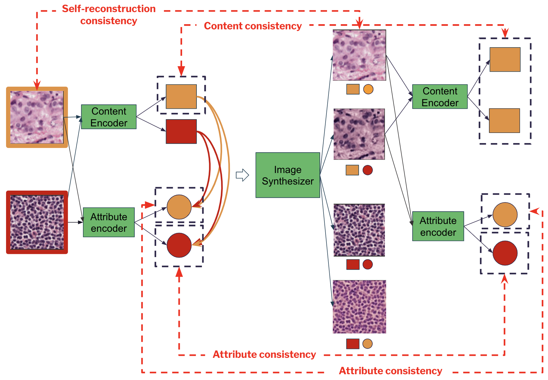
Figure 1: Overview of ContriMix algorithm. Content and attribute tensors are extracted from a batch of images, permuted across samples, and used to generate synthetic images. During training, these images are then passed to the encoders for a second time to extract the content and attributes used in loss calculation. No domain identifiers are used to disentangle between content and attribute.

1.4 ContriMix

We introduce a technique for domain generalization that makes minimal assumptions about the data or its mapping to discrete domains, which we term “ContriMix”. ContriMix is an unsupervised, learnable method to disentangle biological content from incidental attributes for each image.

We design ContriMix keeping the following properties in mind:

1. The method is fully unsupervised, and does not assume the domain of the data. Therefore, it can take advantage of a large body of unlabeled data. The fact that ContriMix does not need domain identifiers during training makes it suitable for applications where either domain-related metadata is not present or multiple types of domains exist whose relative importance is unclear beforehand. The property allows ContriMix to accommodate the fact that variation across samples can be continuous and not just across specific domains, and the dataset can be a mixture of many domains.

2. ContriMix encoders is domain-independent. Only a single model is needed even in the presence of multiple domains. Data from new domains can be introduced and a pretrained ContriMix model can extract attributes from them and use them to generate synthetic images.

3. It is robust to artifacts in whole-slide imaging and allows successful image translation under scanning artifacts, pathologist markers, red blood cells, and other sources of variation.

4. It captures both inter- and intra-domain variation within each domain by operating at patch level instead of coarser levels (e.g., at the whole slide image, collection site, or digitization method levels). To our knowledge, most other deep learning methods define the domain set at a very high and often coarse scale like hospitals and scanners. Therefore, they are not designed to capture finer variation within each domain, such as differences in stain intensity within samples from the same hospital, or differences in tissue thickness due to natural variation in pre-analytic processing.

5. No prior knowledge of the staining or imaging conditions is needed. This requirement allows the use of ContriMix not only in histopathology but also in other modalities like fluorescence and histochemistry imaging.

We conduct experiments to demonstrate the effectiveness of ContriMix for domain generalization in two histopathology datasets, Camelyon17-WILDS [17] and RCC subtyping [31], where it outperforms other state-of-the-art methods. We also perform ablation experiments to understand the hyperparameters and learned representations of ContriMix. Lastly, we demonstrate the effectiveness of ContriMix in a fluorescence microscopy dataset (RxRx1) [38] where ContriMix achieves state-of-the-art results, indicating its applicability in a variety of medical imaging datasets. We make our source code and trained ContriMix encoders available for reproducibility, and pseudo-code is shared in the Appendix.

2 ContriMix algorithm

2.1 Overview

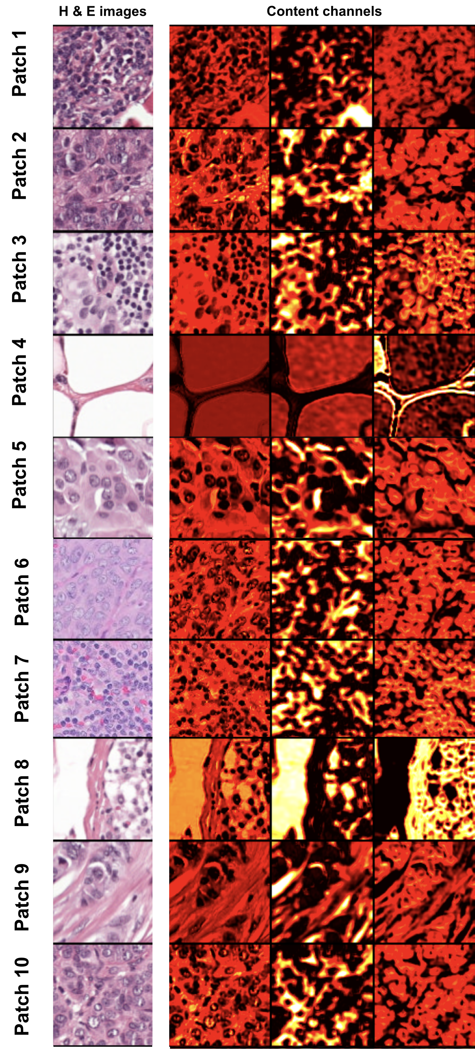
Figure 1: Additional examples of content channel visualizations that were used in the content tensor qualitative study

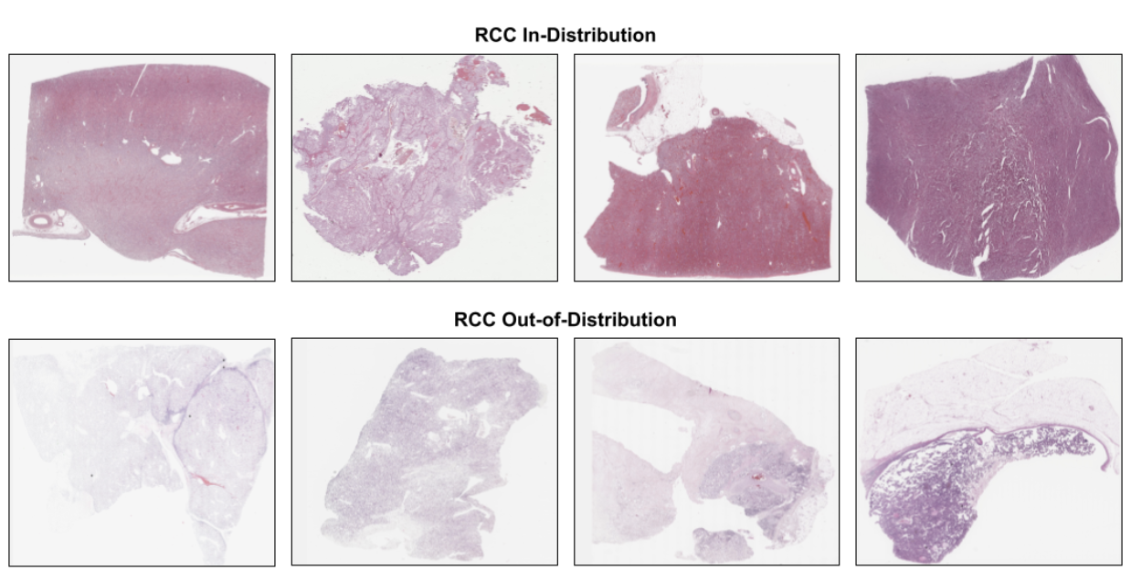
Figure 2: Examples of in-distribution (ID) and out-of-distribution (OOD) WSIs from the RCC cancer subtyping datasets. The first row shows ID TCGA WSIs, while the second row shows WSIs procured from a different lab site and scanner. We can see the variations in tissue preparation and scanning which lead to significant visual differences.

ContriMix solves the problem of unsupervised disentanglement of content and attributes by leveraging synthetic images that have similar content but different attributes. To accomplish this, content and attribute tensors are extracted from input images as shown in Fig. 1. These tensors are then mixed to generate synthetic images. These synthetic images, together with the original images, will be passed again to the content encoder $E^{c}$ and attribute encoder $E^{a}$ to extract output tensors. These output tensors are used in the ContriMix loss to update the weights of the encoders. Example synthetic images generated by ContriMix are shown in Fig. 2.

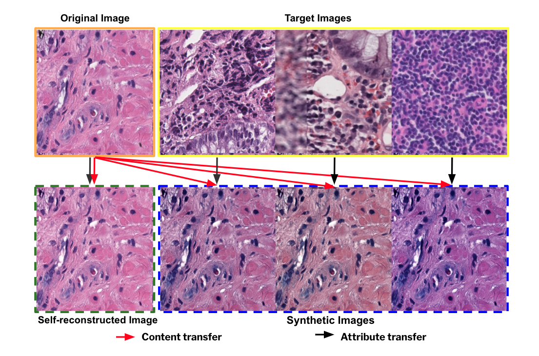
Figure 2: Synthetic images generated by ContriMix on histopathology images. We extract the content from the original image (top-left) and combine it with the attributes of the target images (top-right) to generate the synthetic images (bottom-right). We also use the attribute of the original image with the content of the original image to generate the self-reconstructed image (bottom-left). When extracting the attributes from the target images, any image artifact (e.g., blur) (3rd column, top-row) is ignored by the model.

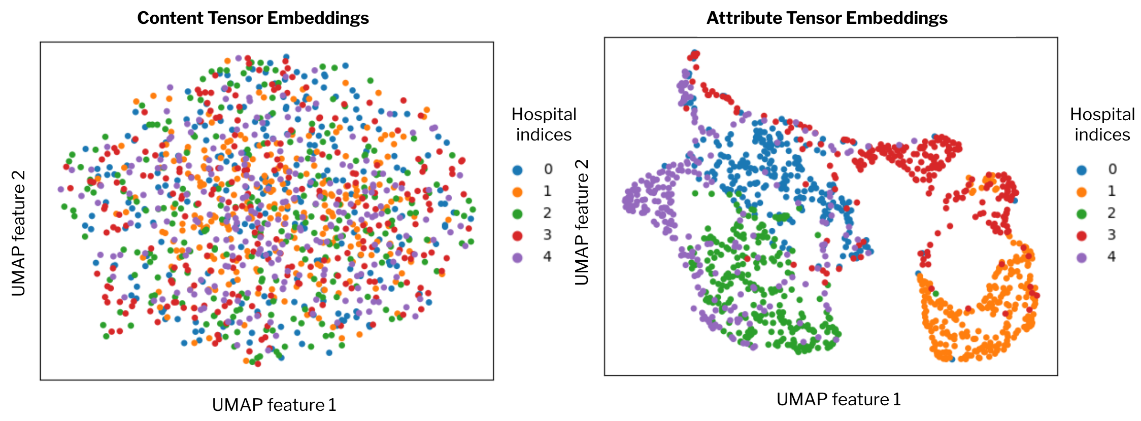
Figure 3: UMAP plot for ContriMix content (left) and attribute (right) tensors colored by different centers for images in Camelyon17-WILDS. The attribute encoder captures the differences across centers without needing any explicit domain supervision, while the content encoder learns center-invariant features.

Let $B=\{x_{1},x_{2},...,x_{N}\}$ denote a set of $N$ training samples in the minibatch with $x_{i}\in\mathbb{R}^{H\times W\times C}$. Here, $H,W,C$ are the height, width, and number of channels, respectively. Let $z^{c}_{i}=E^{c}(x_{i})\in\mathbb{R}^{H\times W\times L}$ and $z^{a}_{i}=E^{a}(x_{i})\in\mathbb{R}^{L\times C}$, be the extracted content and attribute tensors. $L$ is the number of attributes. The image generator $G$ takes both content and attribute tensors as inputs and returns a synthetic image $x^{s}_{i}=G(z^{c}_{i},z^{a}_{i})\in\mathbb{R}^{H\times W\times C}$.

To generate synthetic images, the content tensors of each training sample $z^{c}_{i}$ are combined with $M$ other attribute tensors selected from other samples ${z^{a}_{i1},z^{a}_{i2},...z^{a}_{iM}}$ within the same training mini-batch (or from an external set of samples) to generate synthetic images $x^{s}_{im}=G(z^{c}_{i},z^{a}_{im})$ for $m=1,..,M$. Self-reconstruction images $G(z^{c}_{i},z^{a}_{i})$ are also generated and used in the loss calculation.

ContriMix losses are summarized in (Fig. 1). The ContriMix loss includes

$$\begin{split}L_{ContriMix}=&\lambda_{s}L_{self-recon.}+\lambda_{a}L_{attr.}+\\ &\lambda_{c}L_{cont.},\end{split}$$ (1)

where $L_{attr.},L_{cont.},$ and $L_{self-recon.}$ are the attribute consistency loss, content consistency loss, and the self-reconstruction loss, respectively. $\lambda_{s},\lambda_{a},\lambda_{c}$ are weights of the self-reconstructed consistency loss, attribute consistency loss, and the content consistency loss, satisfying $\lambda_{s}+\lambda_{a}+\lambda_{c}=1$.

• Content consistency loss $L_{cont.}$

  $$L_{cont.}=\frac{1}{NM}\sum_{x_{i}\in B}\sum_{m=1}^{M}{\|E^{c}(x_{i})-E^{c}[G(z^{c},z^{a}_{im})]\|}_{1},$$ (2)

  where we have dropped the summation over the minibatches for brevity. ${\|.\|}_{1}$ denotes the $l_{1}$-norm. This term encourages the consistency between the content extracted from the original image $E^{c}(x^{i})$ and the content extracted from synthetic images $E^{c}[G(z^{c},z^{a}_{im})]$.

• Attribute consistency loss $L_{attr.}$

  $$L_{attr.}=\frac{1}{NM}\sum_{x_{i}\in B}\sum_{m=1}^{M}{\|E^{a}(x_{im})-E^{a}[G(z^{c},z^{a}_{im})]\|}_{1}.$$ (3)

  This term requires the attributes extracted from synthetic images $E^{a}[G(z^{c},z^{a}_{im})]$ to be similar to the attribute tensors that were used to generate the synthetic images $E^{a}(x_{im})$.

• Self-reconstructed consistency loss $L_{self-recon.}$: encourages the self-reconstructed images to be similar to the original images by minimizing the $l_{1}$-norm of their difference.

  $$L_{self-recons.}=\frac{1}{NM}\sum_{x_{i}\in B}{\|x_{i}-G(z^{c}_{i},z^{a}_{i})]\|}_{1}.$$ (4)

3 Experimental setup and results

3.1 Datasets

The Camelyon17-WILDS dataset is a subset of the broader Camelyon17 dataset. It contains 450,000 H&E stained lymph-node scans from 5 hospitals. The objective is to classify medical images of size 96 x 96 pixels as either containing tumor or normal tissue. The training dataset consists of patches from the first 3 hospitals, while the validation and test datasets consist of samples from the 4^th and 5^th hospitals, respectively, considered as out-of-distribution. Due to high variability in test set performance across different seeds, the average test accuracy is reported, along with standard deviation over 10 random seeds.

For WSI-level prediction, we use the problem of prediction of cancer subtypes in renal cell carcinoma (RCC) within The Cancer Genome Atlas (TCGA) [46]. TCGA-RCC has 948 WSIs with three histologic subtypes: 158 WSIs with chromophobe RCC (KICH), 504 WSIs belonging to clear cell RCC (KIRC), and 286 to papillary RCC (KIRP). For the OOD dataset, we use WSIs acquired from an independent laboratory. These WSIs have been acquired with different image processing and laboratory techniques, leading to notable differences in staining appearance and visual characteristics. Some example images highlighting this contrast with TCGA have been shared in the Supplementary section. The class-wise distribution for the OOD dataset is as follows: 46 KICH, 254 KIRC, and 134 KIRP WSIs.

The RxRx1-WILDS dataset [17] contains 3-channel $256\times 256$ fluorescent images of 4 cultured cell lines (HUVEC, RPE, HepG2, and U2OS) from 51 siRNA-treated batches (domains). They are split into training (33), OOD validation (4), and OOD test (14). Each batch contains the same type of cell. The task associated with this dataset is to predict the treatment label out of 1,139 classes for each image.

3.2 Implementation details

For the Camelyon17-WILDS and RxRx1-WILDS datasets, we train ContriMix on the training splits provided in [17]. The baseline performance is borrowed from the WILDS leaderboard. The evaluation methodology is consistent with the one used by prior methods on the respective datasets. We use the same DenseNet architectures used by baseline methods for the backbone in WILDS experiments. The AdamW [23] optimizer with a learning rate of 10^-4 is used. For ContriMix content and attribute encoders, we take inspiration from DRIT++[19], modifying the architecture to eliminate the need for domain discriminators since ContriMix does not need domain identifiers in the data. A dot product operation between the content and the attribute tensors is used as the image generator. We discuss the reason for this decision in the Supplementary Section.

For RCC cancer subtype prediction, we use the Deep Attention Multiple Instance Learning (AB-MIL) [12] as a baseline. Synthetic patches are generated via ContriMix, with the same architectures for encoders and generators as above, and passed along with the original patches to the MIL model. To simulate the scenario of not having access to the OOD dataset at the time of training, we restrict our comparisons with methods that do not require access to domain identifiers or test image data at train time. Consequently, we compare ContriMix with non-deep learning, stain vector-based modified implementation of Macenko method [24] (referred to as ‘StainAug’ in table 2) that uses non-negative least squares for the decomposition [11], and Supervised Contrastive MIL (SC-MIL) [15], which has been shown to improve OOD performance on MIL datasets. All MIL models were trained on non-overlapping patches of size 224 x 224 pixels at a resolution of 1 micron per pixel, with a total of 800k patches extracted approximately. Bag sizes were varied from 24 to 1500, and batch sizes were between 8 and 32. An Imagenet-pretrained ShuffleNet was used as the feature extractor. Augmentations applied included flips, center crops, HSV transforms, and probabilistic grayscaling; the values were kept consistent across all techniques. SC-MIL training was done with a temperature value of 1 [15]. An Adam optimizer with a learning rate of 10^-4 was used for all models.

All training was done on Quadro RTX 8000 GPUs using PyTorch v1.11 and CUDA 10.2. The training time was 12 GPU hours for Camelyon17-WILDS, 96 GPU hours for RxRx1-WILDS, and 16 GPU hours for RCC subtyping.

For hyperparameters used in training, we refer the reader to the code repository.

3.3 Comparison of predictive performance

We compare ContriMix with various methods, and results are presented in Tables 1, 2, and 3. We borrowed the performance numbers from the WILDS leaderboard, selecting only the best-performing methods that did not deviate from the official submission guidelines, sharing the same backbone architecture. For Camelyon17-WILDS and RxRx1-WILDS, the results are aggregated over 10 and 3 seeds, respectively.

ContriMix outperforms other methods in Camelyon17-WILDS in terms of both average accuracy and standard deviation on the test set. With RxRx1-WILDS, ContriMix outperforms the baseline ERM, ARM-BN, and LISA. We emphasize that the SOTA for RxRx1-WILDS is the IID representation method [47] with 23.9 (0.3) OOD val accuracy and 39.2 (0.2) test accuracy. However, that method requires adding an ArcFace [7] loss to the backbone losses to maximize the class separability. To benchmark ContriMix, we compare it with only those methods that use the cross-entropy loss.

For RCC subtyping, exhaustive sampling of patches was done at inference time, and majority vote across bags was used as the WSI level prediction to compute the macro-average F1 score and macro-average 1-vs-rest AUROC. While SC-MIL has the best performance on the ID test set, AB-MIL with ContriMix has the best performance on the OOD test set, highlighting the effectiveness of using ContriMix in the MIL framework.

Table 1: Comparison of predictive performance on Camelyon17-WILDS. The mean and standard deviation (in parenthesis) from 10 random seeds are reported. Only the top-5 methods from the WILDS leaderboard are shown in this table.

# Method	OOD Val Acc. (%)	Test Acc. (%)
ERM	85.8 (1.9)	70.8 (7.2)
IRMX (PAIR Opt)	84.3 (1.6)	74.0 (7.2)
LISA	81.8 (1.4)	77.1 (6.9)
ERM w/ targeted aug	92.7 (0.7)	92.1 (3.1)
ContriMix	91.9 (0.6)	94.6 (1.2)

Table 2: Comparison of predictive performance on RCC subtyping. Mean and standard deviation (in parenthesis) were computed via bootstrapping over 1000 runs on the test set.

# Method	ID Test F1	ID Test AUROC	OOD Test F1	OOD Test AUROC
AB-MIL	87.80 (2.29)	97.78 (0.61)	74.85 (2.42)	91.75 (1.61)
AB-MIL+StainAug	87.46 (2.28)	97.83 (0.68)	72.83 (2.34)	94.59 (1.19)
SC-MIL	90.91 (1.98)	98.07 (0.40)	77.83 (2.39)	95.03 (1.09)
AB-MIL+ContriMix	89.10 (2.12)	97.69 (0.70)	81.23 (2.32)	95.59 (1.27)

Table 3: Comparison of predictive performance on RxRx1-WILDS. The mean and standard deviation (in parenthesis) from 3 random seeds are reported.

# Method	OOD Val Acc. (%)	Test Acc. (%)
ERM	19.4 (0.2)	29.9 (0.4)
ARM-BN	20.9 (0.2)	31.2 (0.1)
LISA	20.1 (0.4)	31.9 (1.0)
ContriMix	23.6 (0.9)	35.0 (0.5)

3.4 Qualitative evaluation of synthetic images

We conducted an expert evaluation of the synthetic images generated by ContriMix. Eighty synthetic image patches were randomly selected and shared with a board-certified pathologist, with the following question -

‘Please evaluate the quality of the synthetic images. Please label the quality as ’NOT SATISFACTORY’ if the synthetic image includes any artifact that was not present in the original image, or changes any biological details in the original image.’

Example images are given in figure 2 with more examples shared in the Supplementary section. The expert feedback is summarized as follows - ‘All the synthetic images are free of artifacts or changes that would hinder pathologic interpretation.’

Figure 4 shows some examples of robust image translation with ContriMix for some corner cases. The source, target, and translated images are shown in the top, middle, and bottom rows, respectively. In the left column, the histology ink is present and shows up in green in the target image. ContriMix was able to correctly extract the color of the target image and use it to transfer the color of the source image without carrying over the effect of the artifact or the histology ink. This ability comes from the fact that ContriMix uses different content channels to capture different biologically relevant substances. The next two columns show another example when there are outlier substances available in the source images but not the target images, such as histology ink (middle column) and red blood cells (right column). The translated images showed not only the correct translation of substances available in both images but also the retention of the colors of the outlier substances. We hypothesize that the colors of these outlier substances come from the biases that the ContriMix attribute encoder learned from training. The values of these biases may have been used for these substances in image translation. This ability offers ContriMix an advantage over the traditional methods that require stain vector extraction such as the Macenko method [25], as discussed in section 1.3.1.

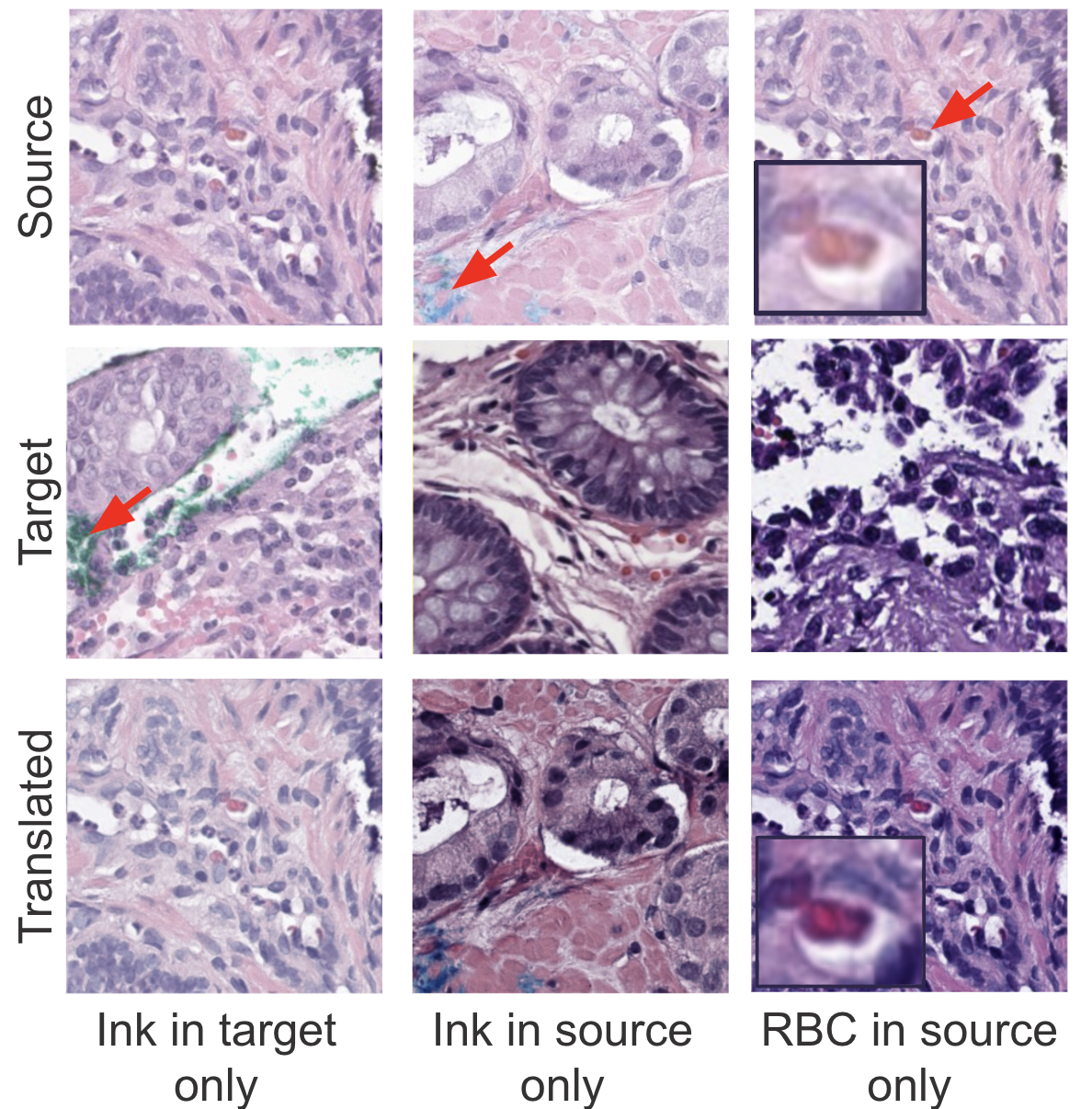
Figure 4: Examples of ‘corner cases’ of image translation successfully performed by ContriMix in when certain artifacts are present only in target image such as histology ink (left column). The middle and right columns show examples of patches that contain artifacts only available in source images not in target images, such as red blood cells and histology ink, respectively. The insets show a zoom-in image of RBCs.

4 Ablation studies

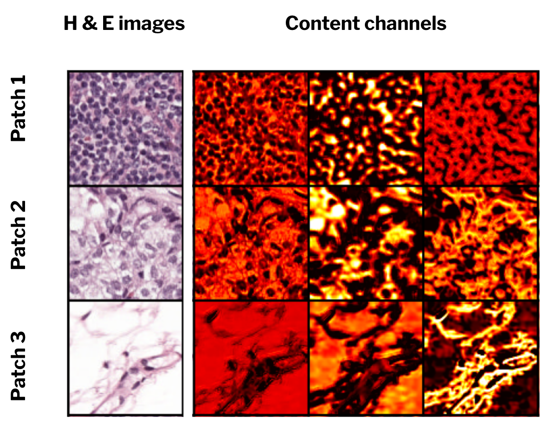
Figure 5: Content channels of ContriMix for three different input images. The left most column contains the original images. The next three columns show three different content channels. ContriMix learns to encode biological information in different channels. Table 5 outlines the biological details in the channels.

Table 4: Ablation experiments for the number of mixes. The mean and standard deviation (in parenthesis) from 10 random seeds are reported.

# Mixes	OOD Val Acc. (%)	Test Acc. (%)
1	92.0 (0.7)	92.4 (3.0)
2	92.2 (0.9)	90.8 (6.1)
3	91.8 (1.1)	93.9 (1.7)
4	91.9 (0.6)	94.6 (1.2)
5	92.4 (0.8)	93.2 (2.3)

4.1 Content tensors

Another qualitative study is conducted to understand what the content channels are learning by visualizing the content channels for 100 patches. These content maps are shared with a board-certified pathologist, who is asked to ascertain a) whether any biological details are being encoded in each channel and b) if yes, what concept(s) they correspond to. An example is shown in Fig. 5, which has 3 rows, one for each image. The left most column shows the original images. The next 3 columns show the extracted content maps. Additional content channels are shared in the Supplementary section. According to the evaluation, different content channels appear to learn various kinds of details, which are tabulated in table 5. No annotations were used in training to teach the model to identify these structures specifically.

Table 5: Expert evaluation of ContriMix content channels and the biological details learned by them.

Content channel	Biological details
1	Cytoplasm, background, connecting tissue
2	Acellular area (Lumen, blood vessel, background)
3	Nuclei, adipose tissue

4.2 Attribute tensors

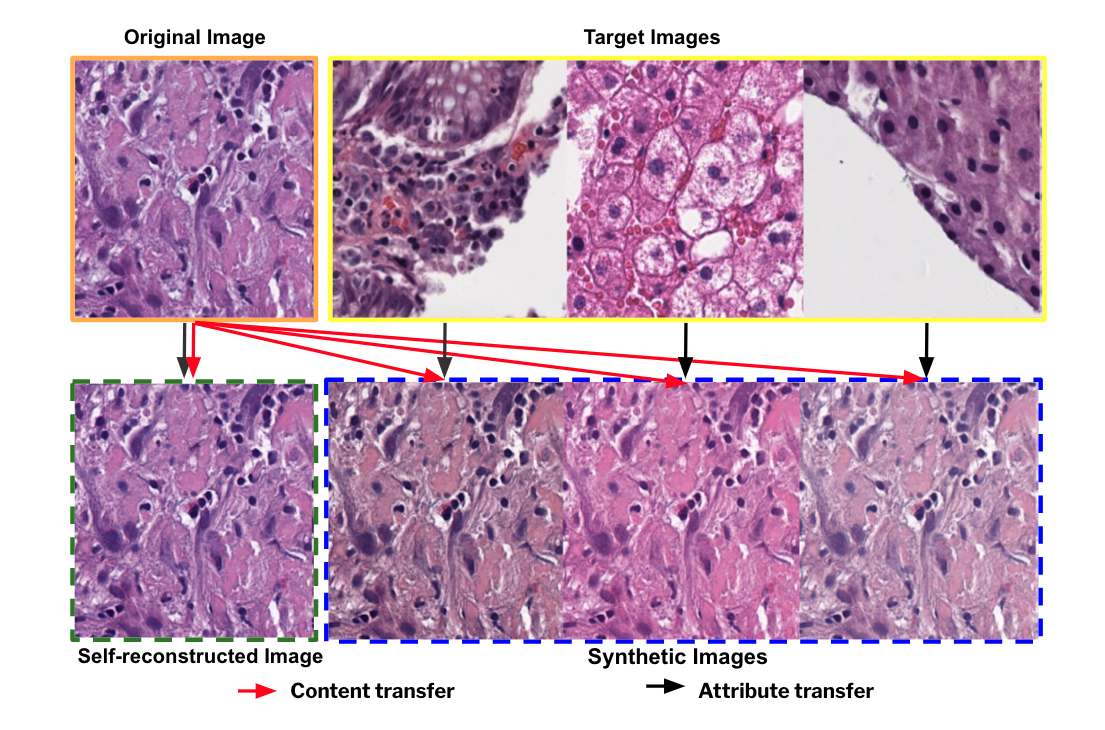
Figure 3: Different examples of synthetic images generated by ContriMix, which were used in the qualitative evaluation study. ContriMix attribute tensors learn to ignore artifacts (e.g.- marker ink, black spots) while the content tensors preserve relevant information without introducing hallucinations. Apart from artifacts, ContriMix is able to account for the presence of background pixels in the input images.

To understand the representations learned by the ContriMix encoder, we pass the content and attribute tensors of 7,200 images of Camelyon17-WILDS extracted by ContriMix to UMAP [27] for dimensionality reduction. Figure 3 shows that the attribute tensors contain the differences across patches from different centers (domains), while the content encoder learns center-invariant features. This happens without having any access to domain supervision during training.

4.3 Number of mixes

Here, we investigate different numbers of mixes (combination of content and attribute tensors to get a synthetic image) $M$, ranging from 1 to 5, with all other hyperparameters fixed. The results in Table 4 indicate that increasing the number of mixes beyond a certain limit (in this case, 4) on Camelyon17-WILDS dataset has no significant effect on the model performance. This finding enables us to use a lower number of mixes and larger batch size at training time.

4.4 Random vs. targeted mixing

The default method of attribute selection for mixing in ContriMix is random over the minibatch. The mixing algorithm does not consider the domain identifiers when selecting an attribute to combine with the content from an image. We ran an experiment to investigate the effect of targeted mixing as opposed to random mixing. In targeted mixing, the domain identifiers of the attributes and content are mutually exclusive. For example, if the content is from domain 1, the attribute can only be chosen from images in domain 2 or 3. Table 6 shows the comparison of random vs targeted mixing on Camelyon17-WILDS dataset. The number of mixes $M$ for this experiment was 4. The experiments are run on 10 random seeds. All other hyper-parameters are the same. Even though there exists a domain imbalance ratio of approximately 1:3 across the training domains, unsupervised random mixing still performs on par with targeted mixing. More experimentation might be required to discover the imbalance level beyond which targeted mixing begins to be more effective. We leave this to future efforts.

Table 6: Ablation experiments for random mixing vs. targeted mixing. The mean and standard deviation (in parenthesis) from 10 random seeds are reported.

Mixing method	OOD Val Acc.(%)	Test Acc.(%)
Random mixing	91.9 (0.6)	94.6 (1.2)
Targeted mixing	91.9 (0.8)	93.7 (1.3)

4.5 Diversity of training domains

The train set of Camelyon17-WILDS contains data from 3 different domains. In this ablation, we remove data belonging to different training domains and study the impact of this on ContriMix. This serves to simulate the real-world setting where we are starved of domain-diverse data. We choose to keep the centers with the least number of samples in the train set - for training with one center, we keep only center 0, while for training with two centers, we keep centers 0 and 3. While there is a drop in performance (7), ContriMix with one center is still able to outperform most methods trained on 3 centers, as seen in Table 1. The results indicate that ContriMix is better able to utilize the intra-dataset variations even in the presence of a single domain.

Table 7: Ablation experiments for number of training centers. We study the impact of dropping entire domains on ContriMix. The mean and standard deviation (in parenthesis) from 10 random seeds are reported.

# Train Centers	OOD Val Acc.(%)	Test Acc.(%)
3	91.9 (0.6)	94.6 (1.2)
2	87.2 (1.3)	88.8 (1.8)
1	85.6 (1.4)	86.9 (4.0)

4.6 Number of attributes

In these experiments, we vary the number of attributes $L$ to study the effect of additional representational capacity in the ContriMix model. The results are reported in Table 8. Increasing the number of attributes helps the model learn until a certain point, beyond which performance starts to saturate.

Table 8: Ablation experiments for varying the number of attributes . The mean and standard deviation (in parenthesis) from 10 random seeds are reported.

# Attributes	OOD Val Acc.(%)	Test Acc.(%)
3	92.1 (1.1)	92.8 (2.2)
5	92.4 (0.9)	93.8 (1.1)
7	91.9 (0.6)	93.1 (0.9)
9	92.7 (1.0)	94.1 (1.4)
11	92.5 (0.8)	93.4 (2.5)
13	92.0 (1.3)	94.1 (1.3)

5 Limitations

Currently, there is no systematic way to determine the optimum number of content and attribute channels for training ContriMix. A larger than necessary number of attributes may lead to an encoding of redundant information, leading to marginal gains in terms of representing true data diversity. In the datasets we experimented with, a simple hyper-parameter search sufficed to generate realistic synthetic images and improve downstream performance, however running this on other image modalities like immunochemistry may yield different results.

6 Conclusion

We introduce ContriMix, a domain generalization technique that does not rely on the presence of domain identifiers. ContriMix generates synthetic images by permuting content and attributes within a set of images. ContriMix achieves comparable or better performance than SOTA methods on three datasets (two from histopathology and one from fluorescence microscopy) without needing domain identifiers during training or testing. Ablation studies indicate the effectiveness of ContriMix for 1) encoding biologically useful information in the content channels, 2) producing domain-invariant representations without needing domain identifiers, and 3) producing competitive results even when trained on data diversity-starved regimes. Thus, ContriMix is a promising technique for domain generalization in microscopy images, with the potential to improve existing digital pathology workflows.

Supplementary Material

1 Using other augmentations with ContriMix

ContriMix can be combined with other augmentations to build a strong augmentation pipeline and further increase the diversity of images for training. We give examples of the augmentations used in Table 9.

Table 9: Augmentations used in ContriMix

Types	Examples
Geometrical transforms	Random flip/rotate, Crop
Resolution / contrast change	Blur, Contrast enhance
Synthetic image generation	CutMix, MixUp, CutOut
Noise, image corruption	Adding noise, color jitter
Normalization	Channel normalization

2 The use of dot product for image generator

In all of our experiments, we use a dot product for the image generator $G$. This is inspired by the physics of histochemistry/fluorescence image formation, since we want to establish a connection between the physically grounded signals and the content and attribute tensors used in ContriMix.

For the histopathology datasets, following the derivation in [33], the optical density can be written as $OD=-log(I/I_{o})=CM$. Here, $C$ is a concentration matrix with each row containing the stain concentration at each pixel. $M$ is a stain vector matrix where rows are the color vectors. $I$ is the raw intensity image obtained from the camera, $I_{o}$ is the background intensity. One can associate content tensor $z^{c}$ and the attribute tensor $z^{a}$ extracted by ContriMix with the stain concentration $C$ and the stain vector matrix $M$ respectively in the optical density equation. Moreover, this model also suggests that a tensor dot product can be used for the image generator $G(z^{c},z^{a})=z^{c}\cdot z^{a}$.

Similarly, with the RxRx1-WILDS fluorescence dataset, the measured intensity can be written as $I=CM$ [28] where $C$ is the concentration (abundance) of the flourophores and $M$ contains the fingerprint of florophores. Hence, the concentration $C$ can be associated with the content tensor $z^{c}$ in ContriMix while the fingerprint can be associated with the the attributes $z^{a}$. Again, a simple dot product operation can be used for the image generator $G$.

3 ContriMix pseudocode

The simplified ContriMix pseudocode (PyTorch-style):

# N: Size of the minibatch
# L: Number of attributes
# M: Number of mixings per image
# E_c: Content encoder
# E_a: Attribute encoder
# G: Image generator
# lambda_s: Self-reconstruction loss weight
# lambda_a: Attribute consistency loss weight
# lambda_c: Content consistency loss weight


# Load a batch with N samples
for b in loader:
    target_idxs = torch.randint(0, N, size=(N, M))
    zc = E_c(b)
    za = E_a(b)

    l1_loss = torch.nn.L1Loss()
    b_sr = G(zc, za)  #Batch self-reconstruction

    sr_loss = l1_loss(b_sr, b) #Self-reconstruction loss

    attr_cons_losses = [l1_loss(E_a(b_sr), z_a)]  #Attribute consistency losses

    cont_cons_losses = [l1_loss(E_c(b_sr), z_c)]  #Content consistency losses

    for mix_idx in range(M):
        za_tgt = za[target_idxs[:, mix_idx]]  #Target attribute for mixing

        b_ct = G(zc, za_target)  # Synthetic image
        attr_cons_losses.append(l1_loss(E_a(b_ct), za_target))
        cont_cons_losses.append(l1_loss(E_c(b_ct), zc))

    # Avergage over the mixing dimension
    attr_loss = torch.mean(torch.stack(attr_cons_losses, dim=0))
    cont_loss = torch.mean(torch.stack(cont_cons_losses, dim=0))


    # Loss
    loss = lambda_s * self_recon_loss + lambda_a * attr_loss + lambda_c * cont_loss

    # Optimization step
    loss.backward()
    optimizer.step()

References

- Bao and Karaletsos [2023] Yujia Bao and Theofanis Karaletsos. Contextual vision transformers for robust representation learning. arXiv preprint arXiv:2305.19402, 2023.
- Bosch et al. [2021] Jaime Bosch, Chuhan Chung, Oscar M Carrasco-Zevallos, Stephen A Harrison, Manal F Abdelmalek, Mitchell L Shiffman, Don C Rockey, Zahil Shanis, Dinkar Juyal, Harsha Pokkalla, et al. A machine learning approach to liver histological evaluation predicts clinically significant portal hypertension in nash cirrhosis. Hepatology, 74(6):3146–3160, 2021.
- Bulten et al. [2020] Wouter Bulten, Hans Pinckaers, Hester van Boven, Robert Vink, Thomas de Bel, Bram van Ginneken, Jeroen van der Laak, Christina Hulsbergen-van de Kaa, and Geert Litjens. Automated deep-learning system for gleason grading of prostate cancer using biopsies: a diagnostic study. The Lancet Oncology, 21(2):233–241, 2020.
- Campanella et al. [2019] Gabriele Campanella, Matthew G Hanna, Luke Geneslaw, Allen Miraflor, Vitor Werneck Krauss Silva, Klaus J Busam, Edi Brogi, Victor E Reuter, David S Klimstra, and Thomas J Fuchs. Clinical-grade computational pathology using weakly supervised deep learning on whole slide images. Nature medicine, 25(8):1301–1309, 2019.
- Chen et al. [2022] Richard J. Chen, Chengkuan Chen, Yicong Li, Tiffany Y. Chen, Andrew D. Trister, Rahul G. Krishnan, and Faisal Mahmood. Scaling vision transformers to gigapixel images via hierarchical self-supervised learning. In Proceedings of the IEEE/CVF Conference on Computer Vision and Pattern Recognition (CVPR), pages 16144–16155, 2022.
- Chen et al. [2020] Ting Chen, Simon Kornblith, Mohammad Norouzi, and Geoffrey Hinton. A simple framework for contrastive learning of visual representations. In Proceedings of the 37th International Conference on Machine Learning. JMLR.org, 2020.
- Deng et al. [2019] Jiankang Deng, Jia Guo, Niannan Xue, and Stefanos Zafeiriou. Arcface: Additive angular margin loss for deep face recognition. In Proceedings of the IEEE/CVF conference on computer vision and pattern recognition, pages 4690–4699, 2019.
- Diao et al. [2021] James A Diao, Jason K Wang, Wan Fung Chui, Victoria Mountain, Sai Chowdary Gullapally, Ramprakash Srinivasan, Richard N Mitchell, Benjamin Glass, Sara Hoffman, Sudha K Rao, et al. Human-interpretable image features derived from densely mapped cancer pathology slides predict diverse molecular phenotypes. Nature communications, 12(1):1–15, 2021.
- Ehteshami Bejnordi et al. [2017] Babak Ehteshami Bejnordi, Mitko Veta, Paul Johannes van Diest, Bram van Ginneken, Nico Karssemeijer, Geert Litjens, Jeroen A. W. M. van der Laak, , and the CAMELYON16 Consortium. Diagnostic Assessment of Deep Learning Algorithms for Detection of Lymph Node Metastases in Women With Breast Cancer. JAMA, 318(22):2199–2210, 2017.
- [10] Irena Gao, Shiori Sagawa, Pang Wei Koh, Tatsunori Hashimoto, and Percy Liang. Out-of-distribution robustness via targeted augmentations. In NeurIPS 2022 Workshop on Distribution Shifts: Connecting Methods and Applications.
- Gullapally et al. [2023] Sai Chowdary Gullapally, Yibo Zhang, Nitin Kumar Mittal, Deeksha Kartik, Sandhya Srinivasan, Kevin Rose, Daniel Shenker, Dinkar Juyal, Harshith Padigela, Raymond Biju, Victor Minden, Chirag Maheshwari, Marc Thibault, Zvi Goldstein, Luke Novak, Nidhi Chandra, Justin Lee, Aaditya Prakash, Chintan Shah, John Abel, Darren Fahy, Amaro Taylor-Weiner, and Anand Sampat. Synthetic domain-targeted augmentation (s-dota) improves model generalization in digital pathology, 2023.
- Ilse et al. [2018] Maximilian Ilse, Jakub Tomczak, and Max Welling. Attention-based deep multiple instance learning. In International conference on machine learning, pages 2127–2136. PMLR, 2018.
- Isola et al. [2017] Phillip Isola, Jun-Yan Zhu, Tinghui Zhou, and Alexei A Efros. Image-to-image translation with conditional adversarial networks. In Proceedings of the IEEE conference on computer vision and pattern recognition, pages 1125–1134, 2017.
- Javed et al. [2022] Syed Ashar Javed, Dinkar Juyal, Harshith Padigela, Amaro Taylor-Weiner, Limin Yu, and aaditya prakash. Additive MIL: Intrinsically interpretable multiple instance learning for pathology. In Advances in Neural Information Processing Systems, 2022.
- Juyal et al. [2023] Dinkar Juyal, Siddhant Shingi, Syed Ashar Javed, Harshith Padigela, Chintan Shah, Anand Sampat, Archit Khosla, John Abel, and Amaro Taylor-Weiner. Sc-mil: Supervised contrastive multiple instance learning for imbalanced classification in pathology, 2023.
- Kang et al. [2021] Hongtao Kang, Die Luo, Weihua Feng, Shaoqun Zeng, Tingwei Quan, Junbo Hu, and Xiuli Liu. Stainnet: a fast and robust stain normalization network. Frontiers in Medicine, 8:746307, 2021.
- Koh et al. [2021] Pang Wei Koh, Shiori Sagawa, Henrik Marklund, Sang Michael Xie, Marvin Zhang, Akshay Balsubramani, Weihua Hu, Michihiro Yasunaga, Richard Lanas Phillips, Irena Gao, et al. Wilds: A benchmark of in-the-wild distribution shifts. In International Conference on Machine Learning, pages 5637–5664. PMLR, 2021.
- Koohbanani et al. [2021] Navid Alemi Koohbanani, Balagopal Unnikrishnan, Syed Ali Khurram, Pavitra Krishnaswamy, and Nasir Rajpoot. Self-path: Self-supervision for classification of pathology images with limited annotations. IEEE Transactions on Medical Imaging, 40(10):2845–2856, 2021.
- Lee et al. [2020a] Hsin-Ying Lee, Hung-Yu Tseng, Qi Mao, Jia-Bin Huang, Yu-Ding Lu, Maneesh Singh, and Ming-Hsuan Yang. Drit++: Diverse image-to-image translation via disentangled representations. Int. J. Comput. Vision, 128(10–11):2402–2417, 2020a.
- Lee et al. [2020b] Hsin-Ying Lee, Hung-Yu Tseng, Qi Mao, Jia-Bin Huang, Yu-Ding Lu, Maneesh Singh, and Ming-Hsuan Yang. Drit++: Diverse image-to-image translation via disentangled representations. International Journal of Computer Vision, 128:2402–2417, 2020b.
- Li et al. [2022] Jin Li, Deepta Rajan, Chintan Shah, Dinkar Juyal, Shreya Chakraborty, Chandan Akiti, Filip Kos, Janani Iyer, Anand Sampat, and Ali Behrooz. Self-training of machine learning models for liver histopathology: Generalization under clinical shifts, 2022.
- Li et al. [2018] Yanghao Li, Naiyan Wang, Jianping Shi, Xiaodi Hou, and Jiaying Liu. Adaptive batch normalization for practical domain adaptation. Pattern Recognition, 80:109–117, 2018.
- Loshchilov and Hutter [2017] Ilya Loshchilov and Frank Hutter. Decoupled weight decay regularization. arXiv preprint arXiv:1711.05101, 2017.
- Macenko et al. [2009a] Marc Macenko, Marc Niethammer, J. S. Marron, David Borland, John T. Woosley, Xiaojun Guan, Charles Schmitt, and Nancy E. Thomas. A method for normalizing histology slides for quantitative analysis. In 2009 IEEE International Symposium on Biomedical Imaging: From Nano to Macro, pages 1107–1110, 2009a.
- Macenko et al. [2009b] Marc Macenko, Marc Niethammer, James S Marron, David Borland, John T Woosley, Xiaojun Guan, Charles Schmitt, and Nancy E Thomas. A method for normalizing histology slides for quantitative analysis. In 2009 IEEE international symposium on biomedical imaging: from nano to macro, pages 1107–1110. IEEE, 2009b.
- Madabhushi and Lee [2016] Anant Madabhushi and George Lee. Image analysis and machine learning in digital pathology: Challenges and opportunities. Medical Image Analysis, 33:170–175, 2016. 20th anniversary of the Medical Image Analysis journal (MedIA).
- McInnes et al. [2018] Leland McInnes, John Healy, and James Melville. Umap: Uniform manifold approximation and projection for dimension reduction. arXiv preprint arXiv:1802.03426, 2018.
- Orth et al. [2018] Antony Orth, Richik N Ghosh, Emma R Wilson, Timothy Doughney, Hannah Brown, Philipp Reineck, Jeremy G Thompson, and Brant C Gibson. Super-multiplexed fluorescence microscopy via photostability contrast. Biomedical optics express, 9(7):2943–2954, 2018.
- Park et al. [2020] Taesung Park, Alexei A Efros, Richard Zhang, and Jun-Yan Zhu. Contrastive learning for unpaired image-to-image translation. In Computer Vision–ECCV 2020: 16th European Conference, Glasgow, UK, August 23–28, 2020, Proceedings, Part IX 16, pages 319–345. Springer, 2020.
- Pérez et al. [2022] José Carlos Gutiérrez Pérez, Daniel Otero Baguer, and Peter Maass. Staincut: Stain normalization with contrastive learning. Journal of Imaging, 8(7), 2022.
- Prasad et al. [2006] Srinivasa R. Prasad, Peter A. Humphrey, Jay R. Catena, Vamsi R. Narra, John R. Srigley, Arthur D. Cortez, Neal C. Dalrymple, and Kedar N. Chintapalli. Common and uncommon histologic subtypes of renal cell carcinoma: Imaging spectrum with pathologic correlation. RadioGraphics, 26(6):1795–1806, 2006. PMID: 17102051.
- Reinhard et al. [2001] Erik Reinhard, Michael Adhikhmin, Bruce Gooch, and Peter Shirley. Color transfer between images. IEEE Computer graphics and applications, 21(5):34–41, 2001.
- Ruifrok et al. [2001] Arnout C Ruifrok, Dennis A Johnston, et al. Quantification of histochemical staining by color deconvolution. Analytical and quantitative cytology and histology, 23(4):291–299, 2001.
- Salehi and Chalechale [2020] Pegah Salehi and Abdolah Chalechale. Pix2pix-based stain-to-stain translation: A solution for robust stain normalization in histopathology images analysis. In 2020 International Conference on Machine Vision and Image Processing (MVIP), pages 1–7. IEEE, 2020.
- Schmitt et al. [2021] Max Schmitt, Roman Christoph Maron, Achim Hekler, Albrecht Stenzinger, Axel Hauschild, Michael Weichenthal, Markus Tiemann, Dieter Krahl, Heinz Kutzner, Jochen Sven Utikal, et al. Hidden variables in deep learning digital pathology and their potential to cause batch effects: prediction model study. Journal of medical Internet research, 23(2):e23436, 2021.
- Schömig-Markiefka et al. [2021] Birgid Schömig-Markiefka, Alexey Pryalukhin, Wolfgang Hulla, Andrey Bychkov, Junya Fukuoka, Anant Madabhushi, Viktor Achter, Lech Nieroda, Reinhard Büttner, Alexander Quaas, et al. Quality control stress test for deep learning-based diagnostic model in digital pathology. Modern Pathology, 34(12):2098–2108, 2021.
- Shaban et al. [2019] M Tarek Shaban, Christoph Baur, Nassir Navab, and Shadi Albarqouni. Staingan: Stain style transfer for digital histological images. In 2019 Ieee 16th international symposium on biomedical imaging (Isbi 2019), pages 953–956. IEEE, 2019.
- Taylor et al. [2019] J. Taylor, B. Earnshaw, B. Mabey, M. Victors, and J. Yosinski. Rxrx1: An image set for cellular morphological variation across many experimental batches. In International Conference on Learning Representations (ICLR), 2019.
- Tellez et al. [2019] David Tellez, Geert Litjens, Péter Bándi, Wouter Bulten, John-Melle Bokhorst, Francesco Ciompi, and Jeroen Van Der Laak. Quantifying the effects of data augmentation and stain color normalization in convolutional neural networks for computational pathology. Medical image analysis, 58:101544, 2019.
- Vahadane et al. [2016] Abhishek Vahadane, Tingying Peng, Amit Sethi, Shadi Albarqouni, Lichao Wang, Maximilian Baust, Katja Steiger, Anna Melissa Schlitter, Irene Esposito, and Nassir Navab. Structure-preserving color normalization and sparse stain separation for histological images. IEEE transactions on medical imaging, 35(8):1962–1971, 2016.
- Voigt et al. [2023] Benjamin Voigt, Oliver Fischer, Bruno Schilling, Christian Krumnow, and Christian Herta. Investigation of semi- and self-supervised learning methods in the histopathological domain. J. Pathol. Inform., 14(100305):100305, 2023.
- Wagner et al. [2021] Sophia J Wagner, Nadieh Khalili, Raghav Sharma, Melanie Boxberg, Carsten Marr, Walter de Back, and Tingying Peng. Structure-preserving multi-domain stain color augmentation using style-transfer with disentangled representations. In Medical Image Computing and Computer Assisted Intervention–MICCAI 2021: 24th International Conference, Strasbourg, France, September 27–October 1, 2021, Proceedings, Part VIII 24, pages 257–266. Springer, 2021.
- Walk [2009] Eric E Walk. The role of pathologists in the era of personalized medicine. Archives of pathology & laboratory medicine, 133(4):605–610, 2009.
- Wang et al. [2016] Dayong Wang, Aditya Khosla, Rishab Gargeya, Humayun Irshad, and Andrew H Beck. Deep learning for identifying metastatic breast cancer. arXiv preprint arXiv:1606.05718, 2016.
- Wang et al. [2021] Dequan Wang, Evan Shelhamer, Shaoteng Liu, Bruno Olshausen, and Trevor Darrell. Tent: Fully test-time adaptation by entropy minimization. In ICLR, 2021.
- Weinstein et al. [2013] John N Weinstein, Eric A Collisson, Gordon B Mills, Kenna R Shaw, Brad A Ozenberger, Kyle Ellrott, Ilya Shmulevich, Chris Sander, and Joshua M Stuart. The cancer genome atlas pan-cancer analysis project. Nature genetics, 45(10):1113–1120, 2013.
- Wu et al. [2022] Jiqing Wu, Inti Zlobec, Maxime Lafarge, Yukun He, and Viktor H Koelzer. Towards iid representation learning and its application on biomedical data. arXiv preprint arXiv:2203.00332, 2022.
- Yao et al. [2022] Huaxiu Yao, Yu Wang, Sai Li, Linjun Zhang, Weixin Liang, James Zou, and Chelsea Finn. Improving out-of-distribution robustness via selective augmentation. In International Conference on Machine Learning, pages 25407–25437. PMLR, 2022.
- Yun et al. [2019] Sangdoo Yun, Dongyoon Han, Seong Joon Oh, Sanghyuk Chun, Junsuk Choe, and Youngjoon Yoo. Cutmix: Regularization strategy to train strong classifiers with localizable features. In Proceedings of the IEEE/CVF international conference on computer vision, pages 6023–6032, 2019.
- Zhang et al. [2017] Hongyi Zhang, Moustapha Cisse, Yann N Dauphin, and David Lopez-Paz. mixup: Beyond empirical risk minimization. arXiv preprint arXiv:1710.09412, 2017.
- Zhu et al. [2017] Jun-Yan Zhu, Taesung Park, Phillip Isola, and Alexei A. Efros. Unpaired image-to-image translation using cycle-consistent adversarial networks. 2017 IEEE International Conference on Computer Vision (ICCV), pages 2242–2251, 2017.