Analysing the Robustness of NSGA-II under Noise

Abstract

Runtime analysis has produced many results on the efficiency of simple evolutionary algorithms like the (1+1) EA, and its analogue called GSEMO in evolutionary multiobjective optimisation (EMO). Recently, the first runtime analyses of the famous and highly cited EMO algorithm NSGA-II have emerged, demonstrating that practical algorithms with thousands of applications can be rigorously analysed. However, these results only show that NSGA-II has the same performance guarantees as GSEMO and it is unclear how and when NSGA-II can outperform GSEMO.

We study this question in noisy optimisation and consider a noise model that adds large amounts of posterior noise to all objectives with some constant probability $p$ per evaluation. We show that GSEMO fails badly on every noisy fitness function as it tends to remove large parts of the population indiscriminately. In contrast, NSGA-II is able to handle the noise efficiently on LeadingOnesTrailingZeroes when $p<1/2$, as the algorithm is able to preserve useful search points even in the presence of noise. We identify a phase transition at $p=1/2$ where the expected time to cover the Pareto front changes from polynomial to exponential. To our knowledge, this is the first proof that NSGA-II can outperform GSEMO and the first runtime analysis of NSGA-II in noisy optimisation.

1 Introduction

Decision making is ubiquitous in everyday life, and often can be formalised as an optimisation problem. In many situations, one may want to examine the trade-off between compromises before making a decision. Sometimes these compromises cannot be accurately evaluated, i. e. due to a lack of available information when a decision has to be made. These two critical but practical settings correspond to the areas Multi-Objective Optimisation (MOO) and Optimisation under Uncertainty (OUU), respectively, which have been studied in both Economics, Operational Research, and Computer Science [4, 7, 29, 33, 34, 43, 47, 51].

MMO is an area where evolutionary multi-objective (EMO) algorithms have shown to be among the most efficient optimisation techniques [50]. Particularly, the Non-dominated Sorting Genetic Algorithm (NSGA-II) is a highly influential framework to build algorithms for MMO, and the original paper [18] is one of the most highly cited papers in evolutionary computation and beyond.

Recently, NSGA-II was analysed by rigorous mathematical means using runtime analysis. In a nutshell, runtime analysis studies the performance guarantees and drawbacks of randomised search heuristics, like Evolutionary Algorithms (EAs), from a Computer Science perspective [35]. The basic approach is to bound the expectation of the random running time $T$ (number of iterations or function evaluations) of a given algorithm on a problem until a global optimum is found in case of a single objective. Extending this to MMO, $T$ is the time to find and cover the whole Pareto front. The algorithm is said to be efficient if this expectation is polynomial in the problem size, and it is inefficient if the expectation is exponential.

Runtime analyses have led to a better understanding of the capabilities and limitations of EAs, for example concerning the advantages of population diversity [15], the benefits of using crossover [21, 49, 10, 41], or the robustness of populations in stochastic optimisation [13, 32, 39, 45]. It can give advice on how to set algorithmic parameters; it was used to identify phase transitions between efficient and inefficient running times for parameters of common selection operators [38], the offspring population size in comma strategies [48] or the mutation rate for difficult monotone pseudo-Boolean functions [23, 42]. Runtime analysis has also inspired novel designs for EAs with practical impacts, e. g. choosing mutation rates from a heavy-tailed distribution to escape from local optima [24], parent selection in steady-state EAs [9], selection in non-elitist populations with power-law ranking [11], or choosing mutation rates adaptively throughout the run [22, 40, 46].

Runtime analyses in MOO started out with the simple SEMO algorithm and the global SEMO (GSEMO) [37, 31]. Both algorithms keep non-dominated solutions in the population. If a new offspring $x$ is created that is not dominated by the current population, it is added to the population and all search points that are weakly dominated by $x$ are removed. Despite its simplicity, it was shown to be effective in AI applications, e. g. [44], where it is called PO(R)SS.

The first theoretical runtime analysis of NSGA-II (without crossover) was performed by Zheng et al. [54]. They showed that NSGA-II covers the whole Pareto front for test functions LOTZ and OMM (see Section 2) in expected $O(\mu n^{2})$ and $O(\mu n\log n)$ function evaluations, respectively, where $\mu$ is the population size and $n$ is the problem size (number of bits). These results require a population of size $\mu\geq 4(n+1)$, hence the best upper bounds are $O(n^{3})$ and $O(n^{2}\log n)$, respectively, that also apply to (G)SEMO [37, 31].

This breakthrough result spawned several very recent papers and already led to several new insights and proposals for improved algorithm designs. Bian and Qian [5] proposed a new parent selection mechanism called stochastic tournament selection and showed that NSGA-II equipped with this operator covers the Pareto front of LOTZ in expected time $O(n^{2})$. Zheng and Doerr [52] proposed to re-compute the crowding distance during the selection process and proved (using LOTZ as a test case) that this improved the spread of individuals on the Pareto front. Doerr and Qu [25] proposed to use heavy-tailed mutations in NSGA-II and quantified the speedup on multimodal test problems. Doerr and Qu [27] and Dang et al. [16] independently demonstrated the advantages of crossover in NSGA-II. In terms of limitations, Zheng and Doerr [53] investigated the inefficiency of NSGA-II for more than two objectives and Doerr and Qu [26] gave lower bounds for the running time of NSGA-II.

Despite these rapidly emerging research works, one important research question remains open. So far all comparisons of NSGA-II with GSEMO show that NSGA-II has the same performance guarantees as GSEMO. Even though NSGA-II is a much more complex algorithm, we do not have an example where NSGA-II was proven to outperform the simple GSEMO algorithm; thus we have not yet unveiled the full potential of NSGA-II.

Here we provide such an example from noisy optimisation.

Our contribution: We show that NSGA-II can drastically outperform GSEMO on a noisy LeadingOnesTrailingZeroes test function. To this end, we introduce a deliberately simple posterior noise model called the $(\delta,p)$-Bernoulli noise model, in which a fixed noise $\delta\in\mathbb{R}$ is added to the fitness in all objectives and in each evaluation with some noise probability $p$. When $\delta$ is positive and sufficiently large, for maximisation problems every noisy solution always dominates every noise-free solution. In this setting, we prove in Theorem 3 that it is difficult for GSEMO to grow its population hence the algorithm is highly inefficient under noise on arbitrary noisy fitness functions. In contrast, for the noise model with a constant $p<1/2$, we show in Theorem 8 that NSGA-II is efficient on the noisy LeadingOnesTrailingZeroes function, if its population size is sufficiently large. This result can be easily extended to other functions. The reason for this performance gap is that NSGA-II keeps dominated solutions in its population while GSEMO immediately removes them. We also prove in Theorem 10 that the behaviour of NSGA-II without crossover dramatically changes for the noise probability slightly above $1/2$, i. e. it suddenly becomes inefficient. Our theoretical results are complemented with empirical results on both the Bernoulli noise model and an additive Gaussian noise, which confirm the advantageous robustness of NSGA-II over GSEMO. As far as we know, this is the first proof that NSGA-II can outperform GSEMO, and the first runtime analysis of NSGA-II under uncertainty.

2 Preliminaries

By $\log(\cdot)$ we denote the logarithm of base 2. $\mathbb{R}$, $\mathbb{Z}$ and $\mathbb{N}$ are the sets of real, integer and natural numbers respectively. For $n\in\mathbb{N}$, define $[n]:=\{1,\dots,n\}$ and $[n]_{0}\coloneqq[n]\cup\{0\}$. We use $\vec{1}$ to denote the all-ones vector $\vec{1}:=(1,\dots,1)$. For a bit string $x:=(x_{1},\dots,x_{n})\in\{0,1\}^{n}$, we use $|x|_{1}$ to denote its number of $1$-bits, i. e. $|x|_{1}=\sum_{i=1}^{n}x_{i}$, and similarly $|x|_{0}$ to denotes its number of zeroes, i. e. $|x|_{0}=\sum_{i=1}^{n}(1-x_{i})=n-|x|_{1}$. We use standard asymptotic notation with symbols $O,\Omega,o$ [8].

This paper focuses on the multi-objective optimisation in a discrete setting, specifically the maximisation of a $d$-objective function $f(x):=(f_{1}(x),\dots,f_{d}(x))$ where $f_{i}\colon\{0,1\}^{n}\rightarrow\mathbb{Z}$ for each $i\in[d]$. We define $f_{\min}:=\min\{f_{i}(x)\mid i\in[d],x\in\{0,1\}^{n}\}$, and $f_{\max}:=\max\{f_{i}(x)\mid i\in[d],x\in\{0,1\}^{n}\}$.

Definition 1.

Consider a $d$-objective function $f$:

• For $x,y\in\{0,1\}^{n}$, we say $x$ weakly dominates $y$ written as $x\succeq y$ (or $y\preceq x$) if $f_{i}(x)\geq f_{i}(y)$ for all $i\in[d]$; $x$ dominates $y$ written as $x\succ y$ (or $y\prec x$) if one inequality is strict.

• A set of points which covers all possible fitness values not dominated by any other points in $f$ is called Pareto front. A single point from the Pareto front is called Pareto optimal.

The weakly-dominance and dominance relations are transitive, e. g. $x\succ y\wedge y\succ z$ implies $x\succ z$. When $d=2$, the function is referred as bi-objective. Two basic bi-objective functions studied in theory of evolutionary computation are LeadingOnesTrailingZeroes and OneMinMax, which can be shortly written as LOTZ and OMM respectively. In $\textsc{LOTZ}(x)\coloneqq(\textsc{LO}(x),\textsc{TZ}(x))$ we count the number $\textsc{LO}(x)$ of leading ones in $x$ (the length of the longest prefix containing only ones) and the number $\textsc{TZ}(x)$ of trailing zeros in $x$ (the length of the longest suffix containing only zeros). OMM minimises and maximises the number of ones: $\textsc{OMM}(x):=(|x|_{1},|x|_{0})$.

1 Initialize $P_{0}\sim\operatorname{Unif}((\{0,1\}^{n})^{\mu})$

2 Partition $P_{0}$ into layers $F^{1}_{0},F^{2}_{0},\dots$ of non-dominated fitnesses, then for each layer $F^{i}_{0}$ compute the crowding distance $\textsc{cDist}(x,F^{i}_{0})$ for each $x\in F^{i}_{0}$

3 for $t:=0\to\infty$ do

4       Initialize $Q_{t}:=\emptyset$

5       for $i:=1\to\mu/2$ do

6             Sample $p_{1}$ and $p_{2}$, each by a binary tournament

7             Sample $u\sim\operatorname{Unif}([0,1])$

8             if $u<p_{c}$ then

9                  Create $s_{1},s_{2}$ by crossover on $p_{1},p_{2}$

10            else

11                  Create $s_{1},s_{2}$ as exact copies of $p_{1},p_{2}$

12            Create $s^{\prime}_{1}$ by bitwise mutation on $s_{1}$ with rate $1/n$

13             Create $s^{\prime}_{2}$ by bitwise mutation on $s_{2}$ with rate $1/n$

14             Update $Q_{t}:=Q_{t}\cup\{s^{\prime}_{1},s^{\prime}_{2}\}$

15            

16      Set $R_{t}:=P_{t}\cup Q_{t}$

17       Partition $R_{t}$ into layers $F^{1}_{t+1},F^{2}_{t+1},\dots$ of non-dominated fitnesses, then for each layer $F^{i}_{t+1}$ compute $\textsc{cDist}(x,F^{i}_{t+1})$ for each $x\in F^{i}_{t+1}$

18       Sort $R_{t}$ lexicographically by $(1/i,\textsc{cDist}(x,F^{i}_{t+1}))$

19       Create the next population $P_{t+1}:=(R[1],\dots,R[\mu])$

20      

Algorithm 1 (NSGA-II Algorithm [18]).

NSGA-II [18, 17] is summarised in Algorithm 1 for bitwise mutation. In each generation, a population $Q_{t}$ of $\mu$ new offspring search points are created through binary tournament, crossover and mutation. The binary tournament in line 1 uses the same criteria as the sorting procedure in line 1 which will be detailed below. The crossover is only applied with some probability $p_{c}\in(0,1)$ to produce two solutions $s_{1},s_{2}$. Otherwise $s_{1},s_{2}$ are the exact copies of the winners of the tournaments. The bitwise mutation on $s_{1},s_{2}$ creates two offspring by flipping each bit of the input independently with probability $1/n$. Our positive result for NSGA-II (Theorem 8) holds for arbitrary crossover operators as it only relies on steps without crossover. To simplify the analysis, we assume that the tournaments for parent selection are performed independently and with replacement.

During the survival selection, the parent and offspring populations $P_{t}$ and $Q_{t}$ are joined into $R_{t}$, and then partitioned into layers $F^{1}_{t+1},F^{2}_{t+1},\dots$ by the non-dominated sorting algorithm [18]. The layer $F^{1}_{t+1}$ consists of all non-dominated points, and $F^{i}_{t+1}$ for $i>1$ only contains points that are dominated by those from $F^{1}_{t+1},\dots,F^{i-1}_{t+1}$. In each layer, the crowding distance is computed for each search point, then the points of $R_{t}$ are sorted with respect to the indices of the layer that they belong to as the primary criterion, and then with the computed crowding distances as the secondary criterion. Only the $\mu$ best solutions of $R_{t}$ form the next population.

Let $M:=(x_{1},x_{2},\dots,x_{|M|})$ be a multi-set of search points. The crowding distance $\textsc{cDist}(x_{i},M)$ of $x_{i}$ with respect to $M$ is computed as follows. At first sort $M$ as $M=(x_{k_{1}},\dots,x_{k_{|{M}|}})$ with respect to each objective $k\in[d]$ separately. Then

$$\textsc{cDist}(x_{i},M) :=\sum_{k=1}^{d}\textsc{cDist}_{k}(x_{i},M),\text{ where }$$ (1)

$$\textsc{cDist}_{k}(x_{k_{i}},M) \!:=\!\begin{cases}\infty\;&\text{if }i\in\{1,|M|\},\\ \frac{f_{k}\left(x_{k_{i-1}}\right)-f_{k}\left(x_{k_{i+1}}\right)}{f_{k}\left(x_{k_{1}}\right)-f_{k}\left(x_{k_{M}}\right)}&\text{otherwise.}\end{cases}\!\!\!\!$$ (2)

The first and last ranked individuals are always assigned an infinite crowding distance. The remaining individuals are then assigned the differences between the values of $f_{k}$ of those ranked directly above and below the search point and normalized by the difference between $f_{k}$ of the first and last ranked.

The GSEMO algorithm is shown in Algorithm 2. Starting from one randomly generated solution, in each generation a new search point $s^{\prime}$ is created by crossover, with some probability $p_{c}\in(0,1)$, and bitwise mutation with parameter $1/n$ afterwards where parents are selected uniformly at random. If $s^{\prime}$ is not dominated by any solutions of the current population $P_{t}$ then it is added to the population, and those weakly dominated by $s^{\prime}$ are removed from the population. The population size $|P_{t}|$ is unrestricted for GSEMO.

1 Initialize $P_{0}:=\{s\}$ where $s\sim\operatorname{Unif}(\{0,1\}^{n})$

2 for $t:=0\to\infty$ do

3       Sample $p_{1}\sim\operatorname{Unif}(P_{t})$

4       Sample $u\sim\operatorname{Unif}([0,1])$

5       if $u<p_{c}$ then

6             Sample $p_{2}\sim\operatorname{Unif}(P_{t})$

7             Create $s$ by crossover between $p_{1}$ and $p_{2}$

8      else

9             Create $s$ as a copy of $p_{1}$

10      Create $s^{\prime}$ by bitwise mutation on $s$ with rate $1/n$

11       if $s^{\prime}$ is not dominated by any individual in $P_{t}$ then

12             Create the next population $P_{t+1}:=P_{t}\cup\{s\}$

13             Remove all $x\in P_{t+1}$ weakly dominated by $s^{\prime}$

14            

15      

Algorithm 2 (GSEMO Algorithm).

Note that GSEMO and NSGA-II are invariant under a translation of the objective function, that is, they behave identically on $f$ and on $f+\vec{c}$ where $\vec{c}$ is a fixed vector.

3 The Posterior Bernoulli Noise Model

Since our aim is to demonstrate that NSGA-II is more robust to noise than GSEMO, we choose the simplest possible noise model under which the desired effects are evident. Our noise model is inspired by concurrent work [36]. Noise can either be present or absent, the strength of the noise is fixed, and noise is applied to all objectives uniformly. Using a simple noise model facilitates a theoretical analysis and simplifies the presentation. We will discuss possible extensions to more realistic noise models, and we will consider one further noise model (posterior Gaussian noise) in our empirical evaluation (Section 7).

In our posterior noise model, instead of optimising the real fitness $f$, the algorithm only has access to a noisy fitness function, denoted as $\tilde{f}$ that may return fitness values obscured by noise.

(This is different to prior noise [12, 14, 28], in which the search point is altered before the fitness evaluation.) In our noise model the fitness is altered by a fixed additive term $\delta\in\mathbb{R}$ in all objectives, with some probability $p>0$. We refer to $|\delta|$ as the noise strength, and $p$ as the noise probability or frequency.

Definition 2.

Given a noise strength $\delta\in\mathbb{R}$ and a noise probability $p\in[0,1]$, the noisy optimisation of a $d$-objective fitness function $f$ under the $(\delta,p)$-Bernoulli noise model has $\tilde{f}$ defined as

$$\tilde{f}(x):=\begin{cases}f(x)+\delta\cdot\vec{1}&\text{with probability }p,\\ f(x)&\text{otherwise.}\end{cases}$$

When $\tilde{f}(x)=f(x)+\delta\cdot\vec{1}$ we call $x$ a noisy search point and otherwise we call it noise-free. Note that the expected fitness vector of any search point $x$ is

$$\mathrm{E}\left[\tilde{f}(x)\right]=f(x)+p\delta\cdot\vec{1}$$

and hence optimising $f$ is equivalent to optimising the expectation of $\tilde{f}$; in other words, this is equivalent to stochastic optimisation [7]. When $p\in\{0,1\}$ the noisy function $\tilde{f}$ is deterministic and equal to $f$ apart from a possible translation by $\delta$ in all objectives, thus NSGA-II and GSEMO will behave the same as operating on $f$.

Since we aim to study the robustness of these original algorithms, we refrain from noise reduction techniques like re-sampling [2, 45, 6].

We assume that noise is drawn independently for all search points in a generation. This reflects a setting where noise is generated from an external source, e. g. disturbances when evaluating the fitness. We assume however that in each generation the noisy fitness values of evaluated individuals are stored temporarily for that generation. So, if the fitness of an individual is queried multiple times in the same generation, the noisy fitness value from the first evaluation in that generation is returned.

Now we obtain a specific noise model by setting $\delta>f_{\max}-f_{\min}$. In this case, noise boosts the fitness of a search point in an extreme way; its fitness immediately strictly dominates that of every noise-free search point. For all $\delta>f_{\max}-f_{\min}$ NSGA-II (or GSEMO) behaves identically on the noise model $(\delta,p)$ as on $(-\delta,1-p)$, because in the latter model the roles of noisy and noise-free search points are swapped and the fitness is translated by $-\delta\cdot\vec{1}$. The latter model corresponds to a setting where noise may destroy the fitness of a search point. This scenario is closely related to practice when optimising problems with constraints that are typically met, but where noise may violate constraints and this incurs a large penalty.

4 GSEMO Struggles With Noise

We show that noise is hugely detrimental for SEMO and GSEMO. Since both algorithms reject all search points that are weakly dominated by a new offspring, if the offspring falsely appears to dominate good quality search points, the latter are being lost straight away. The following analysis shows that, for sufficiently large noise strengths $\delta$, there is a good chance that creating a noisy offspring will remove a fraction of the population, irrespective of the fitness of population members. This makes it impossible to grow the population to a size necessary to cover the Pareto front of a function.

Theorem 3.

Consider GSEMO on an arbitrary fitness function $f$ with noise strength $\delta>f_{\max}-f_{\min}$ and noise probability $0<p<1$. For any functions $t(n),\alpha(n)\in\mathbb{N}$, starting with an arbitrary initial population of size at most $\lceil p\alpha(n)\rceil$, the probability of the population reaching a size of at least $\alpha(n)$ in the first $t(n)$ generations is at most $t(n)\cdot(1-p/2)^{\lfloor(1-p)\alpha(n)\rfloor-1}$ and the expected number of generations is at least $(1-p/2)^{-\lfloor(1-p)\alpha(n)\rfloor+1}$.

Proof.

Let $\mu_{t}\leq\alpha(n)-1$ denote the population size at time $t$. We call a step $t+1$ shrinking if $\mu_{t+1}\leq\lceil p\alpha(n)\rceil+1$. Since GSEMO only adds at most one search point to the population, the condition $\mu_{t}\leq\lceil p\alpha(n)\rceil$ implies a shrinking step since $\mu_{t+1}\leq\mu_{t}+1\leq\lceil p\alpha(n)\rceil+1$. Hence we assume $\mu_{t}\geq\lceil p\alpha(n)\rceil+1$ in the following. A sufficient condition for a shrinking step is to create a noisy offspring and to evaluate at most $\lceil p\alpha(n)\rceil$ parents as noisy. Since the noisy offspring dominates all noise-free search points and GSEMO removes these from the population, only noisy parents may survive. The probability of the offspring being noisy is $p$. Conditional on this event, each of the $\mu_{t}$ search points in the population survives with probability $p$, independently from one another. Then the number of survivors is given by a binomial distribution $\mathrm{Bin}(\mu_{t},p)$. We have

$$\Pr\left(\mathrm{Bin}(\mu_{t},p)\leq\lceil p\alpha(n)\rceil\right)\geq\Pr\left(\mathrm{Bin}(\mu_{t},p)\leq\lceil p\mu_{t}\rceil\right)\geq 1/2$$

since the median of the binomial distribution is at most $\lceil p\mu_{t}\rceil$.

Thus, a shrinking step occurs with probability at least $p/2$. If $\mu_{t}\leq\lceil p\alpha(n)\rceil+1$, the population can only grow to $\alpha(n)$ if there is a sequence of $\alpha(n)-(\lceil p\alpha(n)\rceil+1)=\alpha(n)+\lfloor-p\alpha(n)\rfloor-1=\lfloor(1-p)\alpha(n)\rfloor-1$ steps that are all not shrinking. The probability of such a sequence is at most $(1-p/2)^{\lfloor(1-p)\alpha(n)\rfloor-1}$. If a shrinking step occurs, the population size drops to at most $\lceil p\alpha(n)\rceil+1$ and we can re-iterate the argument. Taking a union bound over the first $t(n)$ steps proves the first claim. Noticing that each attempt to reach a population size of at least $\alpha(n)$ requires at least one evaluation, the expected number of evaluations is bounded by the expectation of a geometric random variable with parameter $(1-p/2)^{\lfloor(1-p)\alpha(n)\rfloor-1}$, which is $(1-p/2)^{-\lfloor(1-p)\alpha(n)\rfloor+1}$. ∎

Processes where the current state shows a multiplicative expected decrease, plus some additive term, were recently analysed in [20]. The expected change of the state was described as negative multiplicative drift with an additive disturbance. Lower bounds are given on the expected time to reach some target value $M$. However, these bounds are linear in $M$, whereas the bounds from Theorem 3 are exponential in the target $\alpha(n)$.

Theorem 3 shows that, if $\alpha(n)$ is chosen as the size of the smallest Pareto set, it takes GSEMO exponential expected time in $\alpha(n)$ to reach a population that covers the whole Pareto front.

Theorem 4.

Consider GSEMO on an arbitrary fitness function $f$ for which every Pareto set has size at least $\alpha(n)$. Then, for every constant $p\in(0,1)$, in the $(f_{\max}-f_{\min}+1,p)$-Bernoulli noise model, the expected time for GSEMO to cover the whole Pareto front is $2^{\Omega(\alpha(n))}$.

Since all Pareto sets of well-known multiobjective test functions have size at least $n+1$, we get the following.

Corollary 5.

For every constant $p\in(0,1)$, in the $(n+1,p)$-Bernoulli noise model the expected time for GSEMO on LeadingOnesTrailingZeroes or OneMinMax to cover the whole Pareto set is $2^{\Omega(n)}$.

We are confident that the arguments in this section extend to other posterior noise models, e. g. adding Gaussian posterior noise. If the noise strength is not too small, there is a good chance that the offspring might be sampled with large positive noise, and then population members with a negative noise contribution may be dominated and be removed as argued above.

Note, however, that to achieve domination, the offspring must be at least as good as a population member in all objectives. In our Bernoulli noise model, we add the same noise of $\delta$ to all objectives. If noise is determined independently for each objective and a value of $\delta$ is added with probability $p$, the offspring is guaranteed to dominate every noise-free population member if noise is applied in all dimensions. For $d$ dimensions, the probability of this event is $p^{d}$. If $d$ and $p$ are both constant, this is only a constant-factor difference, and thus if adding noise uniformly to all objectives yields an exponential lower bound from Theorem 3, the same holds when adding noise independently for each objective.

5 NSGA-II is Robust to Noise if $p<\frac{1}{2}$

For NSGA-II with the Bernoulli noise model, when $\delta$ is sufficiently large, noisy search points do not interfere with the dynamics of non-dominated layers containing noise-free points, i. e. in the calculation of the crowding distances. This is captured by the following concepts, which are illustrated in Figure 1.

Definition 6.

Let $C\in\mathbb{Z},D\in\mathbb{N}_{0}$ be some integers, and let $f(x):=(f_{1}(x),f_{2}(x))$ be a discrete bi-objective function.

• A point $x\in\{0,1\}^{n}$ is called a $(C,D)$-point if $f_{1}(x)=C+\ell\wedge f_{2}(x)=C+m$ for some $\ell,m\in[D]_{0}$.

• A point $x\in\{0,1\}^{n}$ is $(C,D)$-superior if it dominates all $(C,D)$-points, i. e. $f_{1}(x)>C+D\wedge f_{2}(x)>C+D$.

• A multi-set $P$ of points of $f$ is called $(C,D)$-separable if it only contains $(C,D)$-points and $(C,D)$-superior points.

Figure 1: Illustration of $(C,D)$-separable multi-sets. Only the two shaded areas contain search points.

To show that NSGA-II can optimise a function and cover a Pareto front, one has to prove that the progress made so far by the optimisation process is maintained and that Pareto optimal solutions are not being lost in future generations [16, 25, 54]. Such arguments were first used by [54] and later on in [5, 25, 16]. In [16] these arguments were extracted and summarised in a lemma [16, Lemma 7]. We adapt the lemma to our case as follows.

Lemma 7.

Consider two consecutive generations $t$ and $t+1$ of the NSGA-II maximising a bi-objective function $f(x):=(f_{1}(x),f_{2}(x))$ where $f_{i}(x)\colon\{0,1\}^{n}\rightarrow\mathbb{Z}$ for each $i\in\{1,2\}$, and two numbers $C\in\mathbb{Z},D\in\mathbb{N}_{0}$ such that $R_{t}$ (i. e. the joint parent and offspring population) is $(C,D)$-separable. Then we have:

• Any layer $F_{t}^{i}$ composed of only $(C,D)$-points has at most ${4(D+1)}$ individuals with positive crowding distances. The same result holds for layers $F_{t+1}^{i}$ that only have $(C,D)$-points.

• If $R_{t}$ has at most $S$ $(C,D)$-superior points for some $S\in\mathbb{N}_{0}$ and the population size $\mu$ satisfies $\mu\geq 4(D+1)+S$, then the following result holds. If there is a $(C,D)$-point $x\in P_{t}$, then there must exist a $(C,D)$-point $y\in P_{t+1}$ with either $f(y)=f(x)$ or $y\succ x$.

Proof.

The layers of $R_{t}$ (the union of parents and offspring) are separated between those containing $(C,D)$-points and those having the superior ones. The layers of $(C,D)$-superior points are higher ranked (have a lower index) than $(C,D)$-points.

(i) It suffices to prove the result for $F_{t+1}^{i}$ with only $(C,D)$-points of $R_{t}$ then it also holds for the same type of layers in $P_{t},P_{t+1}$ because these populations are sub-multi-sets of $R_{t}$. The remaining proof arguments for (i) are identical to those in the proof of result (i) of Lemma 7 in [16], with their $F_{t}^{1}$ being replaced by our $F_{t+1}^{i}$. Thus we omit it here and refer to [16, Lemma 7] for details.

We note one insight from the proof for later use. The proof shows that for each fitness vector $(a,b)$ of the layer there is at least a point with a positive crowding distance.

(ii) Let $i^{*}$ be the smallest integer such that the layer $F^{i^{*}}_{t+1}$ of $R_{t}$ contains only $(C,D)$-points, i. e. the layers $F^{j}_{t+1}$ with $j<i^{*}$ only contain $(C,D)$-superior-points. The condition on $R_{t}$ means that $\sum_{j<i^{*}}|F_{t+1}^{j}|\leq S$, thus it follows from (i) and $\mu\geq 4(D+1)+S$ that $P_{t+1}$ will contain all search points from $F_{t+1}^{i^{*}}$ with positive crowding distance, in addition to the $(C,D)$-superior points of $R_{t}$.

We have the following cases for the $(C,D)$-point $x$:

Case 1: If none of the $(C,D)$-points of $R_{t}$ dominates $x$, then clearly $x\in F_{t+1}^{i^{*}}$. As remarked at the end of the proof of (i), there must exist a $y\in F_{t+1}^{i^{*}}$ with a positive crowding distance and with $f(y)=f(x)$. Thus $y$ will be kept in $P_{t+1}$.

Case 2: If some of the $(C,D)$-points of $R_{t}$ dominate $x$, then let $y$ be such a point. We may assume that $y$ is not dominated by any other point of $R_{t}$ because if there is a $y^{\prime}\in R_{t}$ dominating $y$, we can choose $y^{\prime}$ instead of $y$ and iterate this argument until a non-dominated point is found. This implies that $y\in F_{t+1}^{i^{*}}$ and as in the previous case, there exists a $y^{\prime}\in F_{t+1}^{i^{*}}$ with a positive crowding distance and with $f(y^{\prime})=f(y)$. Thus $y^{\prime}$ will be kept in $P_{t+1}$ and we have $y^{\prime}\succ x$. ∎

Now we use Lemma 7 to show that NSGA-II can find the Pareto front of LOTZ efficiently when the noise probability is at most a constant less than $1/2$. Roughly speaking, the result shows that with a sufficiently large population, a sub-population of NSGA-II can still evolve its noise-free search points, thus noise has a minimal effect on the optimisation process. For example, $\mu\geq 9(n+1)$ meets the condition for all noisy LOTZ functions with $p\leq 1/4\wedge\delta>n$ or $p\geq 3/4\wedge\delta<-n$. We will use this setting later in our experiments.

Theorem 8.

Consider the $(\delta,p)$-model with noise strength $\delta>n$ and constant noise probability $p\in\left(0,\frac{1}{2(1+c)}\right)$ for some constant ${c>0}$. Then NSGA-II with population size $\mu\geq\frac{4(n+1)}{1-2(1+c)p}$ and $p_{c}\leq 1-2^{-o(n)}$ finds and covers the whole Pareto front of noisy LOTZ in $\mathcal{O}\left(n^{2}/(1-p_{c})\right)$ expected generations and $\mathcal{O}\left(\mu n^{2}/(1-p_{c})\right)$ expected fitness evaluations. The result also holds for the $(-\delta,1-p)$-model using the same conditions.

Proof.

For $\delta>n$, the noise model guarantees that all noisy solutions dominate all noise-free solutions, thus the populations $P_{t},Q_{t}$ and $R_{t}$ are typically $(0,n)$-separable with the superior points being the noisy ones. Lemma 7 (i) with $C=0,D=n$ then implies that there are no more than $4(n+1)$ individuals with positive crowding distances in every layer $F_{t}^{i}$, or $F_{t+1}^{i}$ of noise-free individuals.

Furthermore, in each generation of the algorithm, the expected number of parents in $P_{t}$ that are noise-free after re-evaluation is $(1-p)\mu$, thus by an additive Chernoff bound [19, Theorem 1.10.7], the probability of having at least $(1-(1+c)p)\mu$ noise-free parents and conversely at most $(1+c)p\mu$ noisy ones is at least $1-e^{-2c^{2}p^{2}\mu}=1-e^{-\Omega(n)}$. Similarly, during the evaluation of the offspring $Q_{t}$, with probability $1-e^{-\Omega(n)}$, there are at least $(1-(1+c)p)\mu$ noise-free solutions and at most $(1+c)p\mu$ noisy ones. If either one of these two conditions does not occur during a generation, we refer to this as a bad event. The probability of a bad event is at most $2e^{-\Omega(n)}=e^{-\Omega(n)}$. Given the rarity of bad events, we apply the typical run method with the restart argument, see Chapter 5.6 of [35]. We therefore divide the run of the algorithm into two phases, each phase is associated with a goal. The phases last for at most $T_{1}$ and $T_{2}$ generations respectively, and have the failure probability of at most $p_{1}$ and $p_{2}$ respectively. A failure means that a bad event happens during the random length of a phase. As that the following analysis works for any initial population, such a failure is no worse than restarting the analysis on the resulting population. Under this assumption, the expected number of generations until the Pareto front is covered is at most $(\mathrm{E}\left[T_{1}\right]+\mathrm{E}\left[T_{2}\right])/(1-p_{1}-p_{2})$.

Phase 1: Create a first Pareto optimal solution.

Define $i:=\max\{\textsc{LO}(x)+\textsc{TZ}(x)\mid x\in P_{t}\}$ and note that all Pareto optimal solutions $x$ have $\textsc{LO}(x)+\textsc{TZ}(x)=n$. Thus, the phase is completed once $i=n$. We now consider a point $y\in P_{t}$ so that $\textsc{LO}(y)+\textsc{TZ}(y)=i$ and $y$ has positive crowding distance, to give a lower bound for the probability of increasing $i$ in a generation.

During a binary tournament, the probability of selecting $y$ as the first competitor is $1/\mu$. The probability of the other competitor being a noise-free solution with zero crowding distance is bounded from below as follows. There are at least $(1-(1+c)p)\mu$ noise-free parents in $P_{t}$, and each noise-free layer has at most $4(n+1)$ individuals with positive crowding distances. Thus, the sought probability is at least $(1-(1+c)p)\left(1-\frac{4(n+1)}{\mu}\right)\geq(1-(1+c)p)\left(1-\frac{4}{4/(1-2(1+c)p)}\right)=\Omega(1)$. So, even when $y$ is noise-free the probability of it winning the tournament is at least $2\cdot\Omega(1)\cdot(1/\mu)=\Omega(1/\mu)$ where the factor $2$ accounts for the exchangeable roles of the competitors.

To create an offspring $z$ that dominates $y$ with $\textsc{LO}(z)+\textsc{TZ}(z)\geq i+1$ it suffices to select $y$ as a parent, to skip crossover and to flip one specific bit of $y$ during mutation, while keeping the other bits unchanged (this mutation has probability $1/n\cdot(1-1/n)^{n-1}\geq 1/(en)$). These events occur with probability $s_{i}:=(1-p_{c})(1/en)\cdot\Omega(1/\mu)=\Omega((1-p_{c})/(\mu n))$. During $\mu/2$ offspring productions, the probability of creating such a solution $z$ is $1-(1-s_{i})^{\mu/2}\geq\frac{s_{i}\mu/2}{s_{i}\mu/2+1}=\frac{s_{i}\mu}{s_{i}\mu+2}$, where the inequality follows from [3, Lemma 6].

During survival selection, since we have at most $(1+c)p\mu$ noisy solutions in $P_{t}$ and $Q_{t}$, respectively, there are at most $2(1+c)p\mu$ noisy solutions in $R_{t}=P_{t}\cup Q_{t}$. As the population size $\mu$ satisfies $\mu\geq 2(1+c)p\mu+4(n+1)$, Lemma 7 (ii) with $C=0,D=n,S=2(1+c)p\mu$ first implies that even when no such $z$ individual is created an individual with the same fitness as $y$ always survives to the next generation $P_{t+1}$; in other words, $i$ cannot decrease. Second, when one individual $z$ is created, regardless of whether it is evaluated with noise or not, $z$, or an individual weakly dominating it, survives.

So the expected number of generations of this phase is at most:

$$\mathrm{E}\left[T_{1}\right]\leq\sum_{i=0}^{n-1}\left(1+\frac{2}{s_{i}\mu}\right)=n+\frac{2}{\mu}\sum_{i=0}^{n-1}\mathcal{O}\left(\frac{\mu n}{1-p_{c}}\right)=\mathcal{O}\left(\frac{n^{2}}{1-p_{c}}\right).$$

The failure probability of the phase is bounded from above by the law of total probability and union bounds as $p_{1}\leq\sum_{t=1}^{\infty}\Pr\left(T_{1}=t\right)\cdot te^{-\Omega(n)}=e^{-\Omega(n)}\mathrm{E}\left[T_{1}\right]=o(1)$ since $1-p_{c}=2^{-o(n)}$.

Phase 2: Cover the whole Pareto front.

Now that the population $P_{t}$ contains Pareto-optimal individuals, while the whole Pareto front has not been covered, the population contains a Pareto-optimal individual $y$ with positive crowding distance such that one of the fitness vectors $(\textsc{LO}(y)-1,\textsc{TZ}(y)+1)$ or $(\textsc{LO}(y)+1,\textsc{TZ}(y)-1)$ is not yet present in $f(P_{t})$.

As argued for Phase 1, the probability that during one offspring production, the sequence of operations selection, crossover, and mutation produces an offspring $z$ with a missing fitness vector is at least $s_{i}^{\prime}\coloneqq\Omega((1-p_{c})/(\mu n))$. Again with $\mu/2$ trials, the probability of creating $z$ per generation is $1-(1-s_{i}^{\prime})^{\mu/2}\geq s_{i}^{\prime}\mu/(s_{i}^{\prime}\mu+2)$.

During the survival selection, we again use Lemma 7 (ii) with the same parameters to argue that Pareto optimal fitness vectors will never be removed entirely from the population. There can be at most $n$ missing Pareto optimal fitness vectors to cover, thus the expected number of generations to complete this phase is at most

$$\mathrm{E}\left[T_{2}\right]\leq\sum_{i=1}^{n}\left(1+\frac{2}{s_{i}^{\prime}\mu}\right)=\sum_{i=1}^{n}\left(1+\frac{2}{\mu}\cdot\mathcal{O}\left(\frac{\mu n}{1-p_{c}}\right)\right)=\mathcal{O}\left(\frac{n^{2}}{1-p_{c}}\right).$$

and by a similar argument as in the other phase, we also have $p_{2}=o(1)$ given $1-p_{c}=2^{-o(n)}$.

The total expected number of generations until the Pareto front is covered is bounded from above by $(\mathrm{E}\left[T_{1}\right]+\mathrm{E}\left[T_{2}\right])/(1-p_{1}-p_{2})={\mathcal{O}\left(n^{2}/(1-p_{c})\right)/(1-o(1))}=\mathcal{O}\left(n^{2}/(1-p_{c})\right)$. The bound on the expected number of evaluations follows from the fact that the number of solutions evaluated in each generation is $2\mu=O(\mu)$. ∎

Our analysis can be easily extended to show similar results for other functions. For instance, the expected time to cover the Pareto front of noisy OMM in the same noise model is at most $\mathcal{O}\left(\mu n\log{n}/(1-p_{c})\right)$.

Theorem 9.

Consider the $(\delta,p)$-model with noise strength $\delta>n$ and constant noise probability $p\in\left(0,\frac{1}{2(1+c)}\right)$ for some constant ${c>0}$. Then NSGA-II with population size $\mu\geq\frac{4(n+1)}{1-2(1+c)p}$ and $p_{c}\leq 1-2^{-o(n)}$ covers the whole Pareto front of the noisy OMM function in $\mathcal{O}\left(\frac{n\log{n}}{1-p_{c}}\right)$ expected generations and $\mathcal{O}\left(\frac{\mu n\log{n}}{1-p_{c}}\right)$ expected fitness evaluations. The result also holds for the $(-\delta,1-p)$-model using the same conditions.

Proof.

We follow the same approach as in the proof of Theorem 8, by using the typical run method with the restarting argument, and define the bad events the same way. That is, a bad event occurs in generation $t$ either if more than $(1+c)p\mu$ parents in $P_{t}$ are re-evaluated with noise, or if more than $(1+c)p\mu$ offspring individuals in $Q_{t}$ are evaluated with noise, thus the probability of such an event is at most $2e^{-\Omega(n)}=e^{-\Omega(n)}$. Since any search point is Pareto optimal for OMM, we only have a single phase of covering the Pareto front. Like LOTZ, the noisy OMM function is also $(0,n)$-separable, thus the conditions to apply Lemma 7 (i) are all fulfilled given the same setting for $\mu$.

If the Pareto front is not covered entirely, then there must exist search points $z\notin P_{t}$ next to a search point $y\in P_{t}$ with a positive crowding distance, i. e. $||z|_{1}-|y|_{1}|=1\wedge||z|_{0}-|y|_{0}|=1$. (These events are equivalent for 0-1 strings of equal length.) Let $|y|_{1}=i$ thus $|y|_{0}=n-i$, and we will focus on the case $|z|_{1}=|y|_{1}+1=i+1\wedge|z|_{0}=|y|_{0}-1=n-i-1$ as the reasoning is symmetric in the other case of $|z|_{1}=|y|_{1}-1\wedge|z|_{0}=|y|_{0}+1$. Similar to the argument for LOTZ, with probability $\Omega(1/\mu)$, $y$ is selected as a parent and with probability $1-p_{c}$ it creates an offspring by mutation only. To create such a point $z$ by mutation, it suffices to flip one of the $n-i$ $0$-bits of $y$ to $1$ while keeping the rest of the bits unchanged, and this happens with probability $\frac{n-i}{n}\left(1-\frac{1}{n}\right)^{n-1}=\Omega({\frac{n-i}{n}})$. So, the probability that a search point $z$ is created during one offspring production is $s_{i}:=\Omega(\frac{(1-p_{c})(n-i)}{\mu n})$. With $\mu/2$ offspring productions, the chance of creating a solution $z$ is $1-(1-s_{i})^{\mu/2}\geq\frac{s_{i}\mu/2}{s_{i}\mu/2+1}=\frac{s_{i}\mu}{s_{i}\mu+2}$.

Once a point $z$ is created, then by Lemma 7 (ii), similarly to the case of LOTZ, a search point with fitness $f(z)$ is always kept in the population. Thus, starting from $y$, the expected number of generations to cover fitness vectors $(i+1,n-i-1),(i+2,n-i-2),\dots,(n,0)$, if they do not yet exist in the population, is at most

$$\sum_{k=i}^{n-1}\left(1+\frac{2}{\mu s_{i}}\right)\leq\sum_{k=0}^{n-1}\left(1+\mathcal{O}\left(\frac{2n}{(1-p_{c})(n-i)}\right)\right)=\mathcal{O}\left(\frac{n\log{n}}{1-p_{c}}\right).$$

By symmetry, the same bound holds to cover the fitness vectors $(i-1,n-i+1),(i-2,n-i+2),\dots,(0,n)$. So, the expected number of generations to cover the whole front is no more than $\mathrm{E}\left[T\right]=\mathcal{O}\left(\frac{n\log{n}}{1-p_{c}}\right)$, and the failure probability of the phase is at most $\sum_{t=1}^{\infty}\Pr\left(T=t\right)\cdot te^{-\Omega(n)}=e^{-\Omega(n)}\mathrm{E}\left[T\right]=o(1)$ given $1-p_{c}=2^{-o(n)}$. Thus, the expected runtime of the algorithm is at most $\mathcal{O}\left(\frac{n\log{n}}{1-p_{c}}\right)\cdot\frac{1}{1-o(1)}=\mathcal{O}\left(\frac{n\log{n}}{1-p_{c}}\right)$ generations, or, equivalently, at most $\mathcal{O}\left(\frac{\mu n\log{n}}{1-p_{c}}\right)$ fitness evaluations since only $2\mu$ evaluations are required per generation. ∎

6 Phase Transition for NSGA-II at $p=\frac{1}{2}$

We have seen that, when $\delta>n$, with an appropriate scaling of the population size NSGA-II can handle any constant noise probability $p$ approaching $1/2$ from below. Our result from Theorem 8 does not cover the case $p>1/2$ because when approaching $1/2$ from above, the progress of optimisation has to rely on having a sufficient number of good individuals that are evaluated with noise. The dynamic of the algorithm is therefore different, in fact, the next theorem shows that a noise probability around $p>1/2$ leads to poor results on LOTZ. For the sake of simplicity, we omit crossover and leave an analysis including crossover for future work.

Theorem 10.

Consider the NSGA-II with population size $\mu\in[n+1,\infty)\cap O(n)$ and crossover turned off ($p_{c}=0$) on the noisy LOTZ function with the $(\delta,p)$-noise model. If $\delta>n$ and $p$ is a constant such that $1/2<p<10/19$ then NSGA-II requires $e^{\Omega(n)}$ generations with overwhelming probability to cover the whole Pareto front.

The analysis will show that the number of Pareto-optimal individuals is bounded with overwhelming probability. We first give a bound on the probability of creating a Pareto-optimal individual.

Lemma 11.

Let $F:=\{1^{i}0^{n-i}\mid i\in[n]_{0}\}$ be the Pareto set of LOTZ and consider a standard bit mutation creating $y$ from $x$. Then

$$\Pr\left(y\in F\right)\leq\begin{cases}1/e+3/n&\text{ if $x\in F$}\\ 3/n&\text{ otherwise.}\end{cases}$$

Proof.

We assume $n\geq 3$ as otherwise the claimed probability bound is at least $1$, which is trivial. Starting from a parent $x=1^{i}0^{n-i}\in F$, an offspring in $F$ is created if $x$ is cloned, or if it is mutated into another search point $1^{j}0^{n-j}$ with $j\neq i$. We have $\Pr\left(y=x\right)=(1-1/n)^{n}\leq 1/e$ and $\Pr\left(y=1^{j}0^{n-j}\right)\leq n^{-|i-j|}$ for all $j\in[n]_{0}\setminus\{i\}$ since (depending on whether $j<i$ or $j>i$) either the last $|i-j|$ 1-bits or the first $|i-j|$ 0-bits in $x$ must be flipped. The sum of all probabilities is at most

$$\frac{1}{e}+\sum_{d=1}^{\infty}2n^{-d}=\frac{1}{e}+2\cdot\frac{1/n}{1-1/n}\leq\frac{1}{e}+\frac{3}{n}$$

where the last step used $1/(n-1)\leq 3/(2n)$ for $n\geq 3$.

Now assume $x\notin F$. If the Hamming distance to the closest point in $F$ is at least 2, at least two specific bits must be flipped to create a specific offspring $1^{j}0^{n-j}\in F$. This has probability at most $1/n^{2}$. Taking a union bound over $n+1$ possible values of $j$ yields a probability bound of $(n+1)/n^{2}\leq 2/n$. If $x$ has Hamming distance 1 to some search point $1^{i}0^{n-i}\in F$, it either has a single 0-bit among bits $\{1,\dots,i-1\}$ bits (and an all-zeros suffix) or a single 1-bit among bits $\{i+2,\dots,n\}$ bits (and an all-ones prefix). (Bit positions $i$ and $i+1$ are excluded as otherwise $x\in F$.) In the former case, if the 0-bit is at position $i-1$, $x$ has Hamming distance 1 to both $1^{i}0^{n-i}$ and $1^{i-2}0^{n-i+2}$ and Hamming distance at least 2 to all other search points in $F$. If the 0-bit is at some smaller index, $x$ has Hamming distance at least 2 to all search points in $F\setminus\{1^{i}0^{n-i}\}$. The case of a single 1-bit is symmetric. Hence there are always at most two search points at Hamming distance 1 in $F$, and each one is reached with probability at most $1/n$. To reach any other point in $F$, two bits must be flipped. Taking a union bound over all probabilities yields a probability bound of $2/n+n\cdot 1/n^{2}=3/n$ in this case. ∎

Now we prove Theorem 10.

Proof of Theorem 10.

Recall that, owing to $\delta>n$, all noisy individuals dominate all noise-free ones. The Pareto set of LOTZ is $F:=\{1^{i}0^{n-i}\mid i\in[n]_{0}\}$. We use variables $X_{t}:=|P_{t}\cap F|$ to denote the number of individuals on $F$ in generation $t$. The Pareto front can only be found if $X_{t}\geq|F|=n+1$. It is easy to see that the initial population at time $0$ will have $X_{t}<n+1$ with probability at least $1-e^{-\Omega(n)}$, and we assume that this happens. Since crossover is turned off, in each generation the $\mu$ offspring are created independently by the binary tournament selection, followed by bitwise mutation.

We first find an upper bound $p_{\mathrm{tour}}$ on the probability that an individual in $F$ is returned by an application of tournament selection. A necessary event is to sample at least one of the two competitors from $F$. Each competitor is sampled from $F$ with probability $X_{t}/\mu$. By a union bound, the probability of at least one competitor being from $F$ is at most $2X_{t}/\mu$. Thus, $p_{\mathrm{tour}}\leq 2X_{t}/\mu$.

Starting from a parent $x=1^{i}0^{n-i}\in F$, the probability of the offspring also being in $F$ is at most $1/e+3/n$ by Lemma 11. From a parent $x\notin F$, the probability of creating an offspring on $F$ is at most $3/n$ by Lemma 11. Together, the probability of a parent selection followed by mutation creating a search point in $F$ is at most

$$p_{\mathrm{tour}}(1/e+3/n)+3/n\leq\frac{p_{\mathrm{tour}}}{e}+\frac{6}{n}\eqqcolon q.$$

Let $Y_{t}\coloneqq|Q_{t}\cap F|$ be the number of Pareto optimal points in the offspring population, then $Y_{t}$ can be bounded by a binomial distribution, $Y_{t}\preceq\operatorname{Bin}(\mu,q)$. As $\mu=O(n)$, we have $\mathrm{E}\left[Y_{t}\right]\leq 2X_{t}/e+O(1)$. We analyse the distribution of $X_{t+1}$ and consider two cases:

Case 1: $n/4\leq X_{t}\leq n$. For any constant $\delta\in(0,9e/20-1)$ and a sufficiently large $n$, by a Chernoff bound it holds that

$$\Pr\left(Y_{t}\geq 9X_{t}/10\mid X_{t}\geq n/4\right) \leq\Pr\left(Y_{t}\geq(1+\delta)\left(2X_{t}/e+O(1)\right)\right)$$

$$\leq e^{-2\delta^{2}X_{t}/(3e)-\delta^{2}O(1)}=e^{-\Omega(n)}.$$

Thus the probability of creating more than $9X_{t}/10$ offspring on $F$ is exponentially small. Additionally, since $p$ is a constant below $10/19$ and above $1/2$ by two applications of Chernoff bounds we have the following. The probability of having more than $(10/19)(X_{t}+Y_{t})$ noisy individuals on $F$ is $e^{-\Omega(X_{t}+Y_{t})}=e^{-\Omega(n)}$. The probability of having less than $\mu$ noisy individuals among the $2\mu$ individuals in $R_{t}$ is $e^{-\Omega(\mu)}=e^{-\Omega(n)}$. Since the survival selection only keeps the $\mu$ best among the $2\mu$ individuals, if the latter event does not occur then none of the noise-free individuals will survive to the next generation. Thus, when none of the three events occur, i. e. with a probability of at least $1-e^{-\Omega(n)}$ by a union bound, $X_{t+1}\leq(10/19)(X_{t}+Y_{t})<(10/19)(X_{t}+9X_{t}/10)=X_{t}$. In other words,

$$\Pr\left(X_{t+1}\geq X_{t}\right)=e^{-\Omega(n)}.$$

Case 2: $0\leq X_{t}<n/4$. Since $\mathrm{E}\left[Y_{t}\right]\leq 2X_{t}/e+O(1)\leq n/(2e)+O(1)\eqqcolon m$, we have $\Pr\left(Y_{t}\geq 2m\right)\leq e^{-m/3}=e^{-\Omega(n)}$. This implies $X_{t}+Y_{t}\leq n/4+n/e+O(1)\leq n$ (for $n$ large enough) with probability $1-e^{-\Omega(n)}$. If this happens then $X_{t+1}\leq n$.

Combining these two cases gives that to reach $X_{t}\geq n+1$, an event must occur that has probability $e^{-\Omega(n)}$. The expected time until such an event occurs is $e^{\Omega(n)}$, thus NSGA-II requires at least $e^{\Omega(n)}$ generations in expectation. ∎

7 Experiments

To complement the theoretical results, experiments were conducted to compare the robustness of NSGA-II with GSEMO on LeadingOnesTrailingZeroes and OneMinMax. We considered two noise models, the first is the $(\delta,p)$-Bernoulli noise model using $\delta\coloneqq n+1$ and various noise probabilities $p\in\{2^{-2},2^{-3},\dots,2^{-6}\}\cup\{0.4,0.5,0.6\}\cup\{1-2^{-5},1-2^{-4},1-2^{-3},1-2^{-2}\}$ to cover noise probabilities close to $0,1/2$, and $1$ respectively. In the second model, to investigate in how far our results translate to more general noise models, we consider posterior Gaussian noise as in [30]. The noisy fitness of a search point $x$ is defined as follows, $\operatorname{\mathcal{N}}(0,\sigma^{2})$ denoting the normal distribution with mean $0$ and standard deviation $\sigma$:

$$\tilde{f}(x):=f(x)+\vec{1}\cdot\delta\text{ where }\delta\sim\operatorname{\mathcal{N}}(0,\sigma^{2}).$$

A Gaussian noise is always added to the fitness after evaluation (to all objectives), that is, there is no noise probability in this model. For $\sigma=n$ there is a constant probability of $\tilde{f}(x)\succ\tilde{f}(y)$ for any two search points $x,y$, irrespective of their true fitness. Hence we vary the standard deviation as $\sigma:=n\cdot q$ where $q\in\{2^{0},2^{-1},2^{-3},2^{-4}\}$.

We used problem size $n\in\{20,30,40\}$, $p_{c}=0.9$ and one-point crossover. For NSGA-II, the population size is set to $\mu=9(n+1)$. For each experiment, 50 runs were performed. In each run, the algorithm is stopped either when the whole Pareto front is covered and then the number of iterations is recorded, or when the number of fitness evaluations exceeded $10n^{3}$.

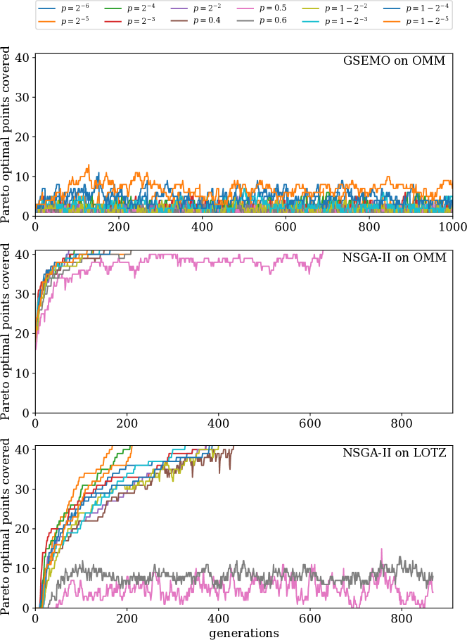
Figure 2: Number of Pareto optimal points covered per generation by GSEMO and NSGA-II on LOTZ, OMM with $n=40$ under the Bernoulli-$(n+1,p)$ noise model in single runs.

As predicted by our results from Section 4, GSEMO failed to cover the Pareto front of both functions within the time limit in all experiments. The first plot of Figure 2 shows the number of different points on the Pareto front of OMM being covered by GSEMO over time for single run on the Bernoulli noise model. This number never exceeds 16, which is below $40\%$ of the size of the Pareto front. This is for the easier function OMM; on LOTZ the maximum value was 4, that is, less than 10% of the front size (plot is omitted for lack of space). The same issue is also evident in the last plot of the figure for NSGA-II on LOTZ with the noise probabilities $p=0.5$ and $p=0.6$. The success rate (fraction of runs covering the Pareto front) was always 100% for NSGA-II in all settings, except for $p\in\{0.5,0.6\}$ on LOTZ, where it was 0%. This is aligned with our theoretical prediction (Theorem 10) there is a phase transition at $p=1/2$ for NSGA-II. Note that in the experiments $p_{c}=0.9$ and Theorem 10 is for $p_{c}=0$ and only claims the negative effect for $p<10/19$ which is below $0.6$. The empirical results thus suggest that the findings extend beyond the setting from Theorem 10.

	LOTZ			OMM
$p$	$n=20$	$n=30$	$n=40$	$n=20$	$n=30$	$n=40$
$2^{-6}$	24090	84051	202822	12346	35982	79927
$2^{-5}$	23317	93687	208128	10273	36706	85786
$2^{-4}$	24919	92294	218483	12987	41440	82101
$2^{-3}$	27898	93297	212550	12686	37987	80848
$2^{-2}$	31856	109701	273906	14684	37235	93562
$0.4$	34212	119540	313298	16041	48848	89887
$0.5$	80301	270145	640453	29160	95859	215240
$0.6$	80301	270145	640453	18604	50826	121581
$1-2^{-2}$	35230	156015	470869	14194	51884	99495
$1-2^{-3}$	29274	102933	221579	14948	43529	97910
$1-2^{-4}$	28350	89008	236429	12572	37402	93341
$1-2^{-5}$	25692	85917	216972	11705	39881	88440

Table 1: Average running time of NSGA-II on LOTZ and OMM under the $(n+1,p)$-Bernoulli noise model. Runs were stopped after $10n^{3}$ evaluations. The success rate was always 100%, except for the shaded cells, where it was 0%.

	LOTZ			OMM
$\sigma$	$n=20$	$n=30$	$n=40$	$n=20$	$n=30$	$n=40$
$n\cdot 2^{-4}$	100%	100%	100%	100%	100%	100%
$n\cdot 2^{-3}$	100%	100%	96%	100%	100%	70%
$n\cdot 2^{-2}$	65%	7%	10%	40%	7%	4%
$n\cdot 2^{-1}$	0%	0%	0%	0%	0%	0%
$n\cdot 2^{0}$	0%	0%	0%	0%	0%	0%

Table 2: Average success rate of NSGA-II on LOTZ and OMM under the Gaussian noise model.

Table 2 shows the average number of fitness evaluations when running NSGA-II on LOTZ, under the Bernoulli noise model. We see that the average running time increases as $p$ approaches $1/2$ and that it decreases when approaching $p=0$ or $1$. With the Gaussian noise model, NSGA-II is only able to cover the Pareto front of the noisy functions when the standard deviation of the noise is small, i. e. $\sigma\in\{n\cdot 2^{-4},n\cdot 2^{-3}\}$. Table 2 shows the success rate of NSGA-II under Gaussian noise. While NSGA-II is effective for small Gaussian noise, it starts to fail when the standard deviation is increased.

8 Conclusions

We have given a first example on which NSGA-II provably outperforms GSEMO and performed a first theoretical runtime analysis of EMO algorithms in stochastic optimisation. While GSEMO is very sensitive to noise, NSGA-II can cope well with noise, even when the noise strength is so large that we have domination between noisy and noise-free search points. This holds when the population size is large enough to enable useful search points to survive and when the noise probability is less than $1/2$. However, for noise probabilities slightly larger than $1/2$, even NSGA-II requires exponential expected runtime, thus it experiences a phase transition at $p=1/2$.

There are many open questions for future work. What if noise is applied to all objectives independently? Can theoretical results be shown for other noise models like Gaussian posterior noise? What mechanisms can prevent noise from disrupting NSGA-II?

References

- [1]
- Akimoto et al. [2015] Youhei Akimoto, Sandra Astete-Morales, and Olivier Teytaud. 2015. Analysis of Runtime of Optimization Algorithms for Noisy Functions over Discrete Codomains. Theoretical Computer Science 605 (2015), 42–50.
- Badkobeh et al. [2015] Golnaz Badkobeh, Per Kristian Lehre, and Dirk Sudholt. 2015. Black-box Complexity of Parallel Search with Distributed Populations. In Proceedings of the Foundations of Genetic Algorithms (FOGA’15). ACM Press, 3–15.
- Ben-Tal et al. [2009] Aharon Ben-Tal, Laurent El Ghaoui, and Arkadi Nemirovski. 2009. Robust Optimization. Princeton University Press.
- Bian and Qian [2022] Chao Bian and Chao Qian. 2022. Better Running Time of the Non-dominated Sorting Genetic Algorithm II (NSGA-II) by Using Stochastic Tournament Selection. In Proceedings of the International Conference on Parallel Problem Solving from Nature (PPSN ’22) (LNCS, Vol. 13399). Springer, 428–441.
- Bian et al. [2021] Chao Bian, Chao Qian, Yang Yu, and Ke Tang. 2021. On the Robustness of Median Sampling in Noisy Evolutionary Optimization. Science China Information Sciences 64, 5 (2021).
- Birge and Louveaux [2011] John R. Birge and Francois Louveaux. 2011. Introduction to Stochastic Programming. Springer.
- Cormen et al. [2009] Thomas H. Cormen, Charles E. Leiserson, Ronald L. Rivest, and Clifford Stein. 2009. Introduction to Algorithms (3rd ed.). The MIT Press.
- Corus et al. [2021] Dogan Corus, Andrei Lissovoi, Pietro S. Oliveto, and Carsten Witt. 2021. On Steady-State Evolutionary Algorithms and Selective Pressure: Why Inverse Rank-Based Allocation of Reproductive Trials Is Best. ACM Transactions on Evolutionary Learning and Optimization 1, 1 (2021), 1–38.
- Corus and Oliveto [2018] Dogan Corus and Pietro S. Oliveto. 2018. Standard Steady State Genetic Algorithms Can Hillclimb Faster Than Mutation-Only Evolutionary Algorithms. IEEE Transactions on Evolutionary Computation 22, 5 (2018), 720–732.
- Dang et al. [2022] Duc-Cuong Dang, Anton V. Eremeev, Per Kristian Lehre, and Xiaoyu Qin. 2022. Fast Non-elitist Evolutionary Algorithms With Power-Law Ranking Selection. In Proceedings of the Genetic and Evolutionary Computation Conference (GECCO ’22). ACM Press, 1372–1380.
- Dang and Lehre [2014] Duc-Cuong Dang and Per Kristian Lehre. 2014. Evolution under Partial Information. In Proceedings of the Genetic and Evolutionary Computation Conference GECCO ’14. ACM Press, 1359–1366.
- Dang and Lehre [2015] Duc-Cuong Dang and Per Kristian Lehre. 2015. Efficient Optimisation of Noisy Fitness Functions with Population-based Evolutionary Algorithms. In Proceedings of the Foundations of Genetic Algorithms (FOGA ’15). ACM Press, 62–68.
- Dang and Lehre [2016] Duc-Cuong Dang and Per Kristian Lehre. 2016. Runtime Analysis of Non-elitist Populations: From Classical Optimisation to Partial Information. Algorithmica 75, 3 (2016), 428–461.
- Dang et al. [2017] Duc-Cuong Dang, Tobias Friedrich, Timo Kötzing, Martin S. Krejca, Per Kristian Lehre, Pietro S. Oliveto, Dirk Sudholt, and Andrew M. Sutton. 2017. Escaping Local Optima Using Crossover with Emergent Diversity. IEEE Transactions on Evolutionary Computation 22 (2017), 484–497. Issue 3.
- Dang et al. [2023] Duc-Cuong Dang, Andre Opris, Bahare Salehi, and Dirk Sudholt. 2023. A Proof that Using Crossover Can Guarantee Exponential Speed-Ups in Evolutionary Multi-Objective Optimisation. In Proceedings of the AAAI Conference on Artificial Intelligence, AAAI 2023. AAAI Press, to appear, preprint available at http://arxiv.org/abs/2301.13687.
- Deb [2011] Kalyanmoy Deb. 2011. NSGA-II Source Code in C, version 1.1.6. https://www.egr.msu.edu/~kdeb/codes/nsga2/nsga2-gnuplot-v1.1.6.tar.gz. Accessed: 2022-08-15.
- Deb et al. [2002] Kalyanmoy Deb, Amrit Pratap, Sameer Agarwal, and T. Meyarivan. 2002. A Fast and Elitist Multiobjective Genetic Algorithm: NSGA-II. IEEE Transactions on Evolutionary Computation 6, 2 (2002), 182–197.
- Doerr [2020] Benjamin Doerr. 2020. Probabilistic Tools for the Analysis of Randomized Optimization Heuristics. In Theory of Evolutionary Computation: Recent Developments in Discrete Optimization, Benjamin Doerr and Frank Neumann (Eds.). Springer, 1–87.
- Doerr [2021] Benjamin Doerr. 2021. Lower Bounds for Non-elitist Evolutionary Algorithms via Negative Multiplicative Drift. Evolutionary Computation 29, 2 (06 2021), 305–329.
- Doerr et al. [2015] Benjamin Doerr, Carola Doerr, and Franziska Ebel. 2015. From Black-Box Complexity to Designing New Genetic Algorithms. Theoretical Computer Science 567 (2015), 87–104.
- Doerr et al. [2019] Benjamin Doerr, Christian Gießen, Carsten Witt, and Jing Yang. 2019. The (1+) Evolutionary Algorithm with Self-Adjusting Mutation Rate. Algorithmica 81, 2 (2019), 593–631.
- Doerr et al. [2013] Benjamin Doerr, Thomas Jansen, Dirk Sudholt, Carola Winzen, and Christine Zarges. 2013. Mutation Rate Matters Even When Optimizing Monotonic Functions. Evolutionary Computation 21, 1 (2013), 1–21.
- Doerr et al. [2017] Benjamin Doerr, Huu Phuoc Le, Régis Makhmara, and Ta Duy Nguyen. 2017. Fast Genetic Algorithms. In Proceedings of the Genetic and Evolutionary Computation Conference (GECCO ’17). ACM Press, 777–784.
- Doerr and Qu [2022] Benjamin Doerr and Zhongdi Qu. 2022. A First Runtime Analysis of the NSGA-II on a Multimodal Problem. In Proceedings of the International Conference on Parallel Problem Solving from Nature (PPSN ’22) (LNCS, Vol. 13399). Springer, 399–412.
- Doerr and Qu [2023a] Benjamin Doerr and Zhongdi Qu. 2023a. From Understanding the Population Dynamics of the NSGA-II to the First Proven Lower Bounds. In Proceedings of the AAAI Conference on Artificial Intelligence, AAAI 2023. AAAI Press, to appear, preprint available at https://arxiv.org/abs/2209.13974.
- Doerr and Qu [2023b] Benjamin Doerr and Zhongdi Qu. 2023b. Runtime Analysis for the NSGA-II: Provable Speed-Ups From Crossover. In Proceedings of the AAAI Conference on Artificial Intelligence, AAAI 2023. AAAI Press, to appear, preprint available at https://arxiv.org/abs/2208.08759.
- Droste [2004] Stefan Droste. 2004. Analysis of the (1+1) EA for a Noisy OneMax. In Proceedings of the Genetic and Evolutionary Computation Conference (GECCO ’04). Springer, 1088–1099.
- Forman and Selly [2001] Ernest H Forman and Mary Ann Selly. 2001. Decision by Objectives: How to Convince Others That You are Right. World Scientific Publishing.
- Friedrich et al. [2017] Tobias Friedrich, Timo Kötzing, Martin S. Krejca, and Andrew M. Sutton. 2017. The Compact Genetic Algorithm is Efficient Under Extreme Gaussian Noise. IEEE Transactions on Evolutionary Computation 21, 3 (2017), 477–490.
- Giel and Lehre [2010] Oliver Giel and Per Kristian Lehre. 2010. On the Effect of Populations in Evolutionary Multi-Objective Optimisation. Evolutionary Computation 18, 3 (2010), 335–356.
- Gießen and Kötzing [2016] Christian Gießen and Timo Kötzing. 2016. Robustness of Populations in Stochastic Environments. Algorithmica 75, 3 (2016), 462–489.
- Goh and Tan [2007] Chi Keong Goh and Kay Chen Tan. 2007. An Investigation on Noisy Environments in Evolutionary Multiobjective Optimization. IEEE Transactions on Evolutionary Computation 11, 3 (2007), 354–381.
- Hughes [2001] Evan J. Hughes. 2001. Evolutionary Multi-objective Ranking with Uncertainty and Noise. In Proceedings of the First International Conference on Evolutionary Multi-Criterion Optimization (EMO 2001) (LNCS, Vol. 1993). Springer, 329–343.
- Jansen [2013] Thomas Jansen. 2013. Analyzing Evolutionary Algorithms - The Computer Science Perspective. Springer.
- Jorritsma et al. [2023] Joost Jorritsma, Johannes Lengler, and Dirk Sudholt. 2023. Comma Selection Outperform Plus Selection on OneMax with Randomly Planted Optima. In Proceedings of the Genetic and Evolutionary Computation Conference (GECCO ’23). ACM Press, to appear.
- Laumanns et al. [2004] Marco Laumanns, Lothar Thiele, and Eckart Zitzler. 2004. Running Time Analysis of Multiobjective Evolutionary Algorithms on Pseudo-Boolean Functions. IEEE Transactions on Evolutionary Computation 8, 2 (2004), 170–182.
- Lehre [2011] Per Kristian Lehre. 2011. Negative Drift in Populations. In Proceedings of the International Conference on Parallel Problem Solving from Nature (PPSN ’10) (LNCS, Vol. 6238). Springer, 244–253.
- Lehre and Qin [2021] Per Kristian Lehre and Xiaoyu Qin. 2021. More Precise Runtime Analyses of Non-elitist EAs in Uncertain Environments. In Proceedings of the Genetic and Evolutionary Computation Conference (GECCO ’21). ACM, 1160–1168.
- Lehre and Qin [2022] Per Kristian Lehre and Xiaoyu Qin. 2022. Self-Adaptation via Multi-Objectivisation: A Theoretical Study. In Proceedings of the Genetic and Evolutionary Computation Conference (GECCO ’22). ACM, 1417–1425.
- Lengler [2020] Johannes Lengler. 2020. A General Dichotomy of Evolutionary Algorithms on Monotone Functions. IEEE Transactions on Evolutionary Computation 24, 6 (2020), 995–1009.
- Lengler and Steger [2018] Johannes Lengler and Angelika Steger. 2018. Drift Analysis and Evolutionary Algorithms Revisited. Combinatorics, Probability and Computing 27, 4 (2018), 643–666.
- Llorà and Goldberg [2003] Xavier Llorà and David E. Goldberg. 2003. Bounding the Effect of Noise in Multiobjective Learning Classifier Systems. Evolutionary Computation 11, 3 (2003), 278–297.
- Qian et al. [2020] Chao Qian, Chao Bian, and Chao Feng. 2020. Subset Selection by Pareto Optimization with Recombination. In Proceedings of the AAAI Conference on Artificial Intelligence, AAAI 2020. AAAI Press, 2408–2415.
- Qian et al. [2021] Chao Qian, Chao Bian, Yang Yu, Ke Tang, and Xin Yao. 2021. Analysis of Noisy Evolutionary Optimization When Sampling Fails. Algorithmica 83, 4 (2021), 940–975.
- Qin and Lehre [2022] Xiaoyu Qin and Per Kristian Lehre. 2022. Self-Adaptation via Multi-objectivisation: An Empirical Study. In Proceedings of the International Conference on Parallel Problem Solving from Nature (PPSN ’22) (LNCS, Vol. 13398). Springer, 308–323.
- Ravi et al. [1993] R. Ravi, Madhav V. Marathe, S. S. Ravi, Daniel J. Rosenkrantz, and Harry B. Hunt III. 1993. Many Birds With One Stone: Multi-Objective Approximation Algorithms. In Proceedings of the Annual ACM Symposium on Theory of Computing (STOC ’93). ACM Press, 438–447.
- Rowe and Sudholt [2014] Jonathan E. Rowe and Dirk Sudholt. 2014. The choice of the offspring population size in the (1,) evolutionary algorithm. Theoretical Computer Science 545 (2014), 20–38.
- Sudholt [2017] Dirk Sudholt. 2017. How Crossover Speeds Up Building-Block Assembly in Genetic Algorithms. Evolutionary Computation 25, 2 (2017), 237–274.
- Tan et al. [2005] Kay Chen Tan, Eik Fun Khor, and Tong Heng Lee. 2005. Multiobjective Evolutionary Algorithms and Applications. Springer.
- Teich [2001] Jürgen Teich. 2001. Pareto-Front Exploration with Uncertain Objectives. In Proceedings of the First International Conference on Evolutionary Multi-Criterion Optimization (EMO 2001) (LNCS, Vol. 1993). Springer, 314–328.
- Zheng and Doerr [2022a] Weijie Zheng and Benjamin Doerr. 2022a. Better Approximation Guarantees for the NSGA-II by Using the Current Crowding Distance. In Proceedings of the Genetic and Evolutionary Computation Conference (GECCO ’22). ACM Press, 611–619.
- Zheng and Doerr [2022b] Weijie Zheng and Benjamin Doerr. 2022b. Runtime Analysis for the NSGA-II: Proving, Quantifying, and Explaining the Inefficiency For Many Objectives. https://arxiv.org/abs/2211.13084
- Zheng et al. [2022] Weijie Zheng, Yufei Liu, and Benjamin Doerr. 2022. A First Mathematical Runtime Analysis of the Non-dominated Sorting Genetic Algorithm II (NSGA-II). In Proceedings of the AAAI Conference on Artificial Intelligence, AAAI 2022. AAAI Press, 10408–10416.