TESS and CHEOPS Discover Two Warm Sub-Neptunes Transiting the Bright K-dwarf HD 15906

Abstract

We report the discovery of two warm sub-Neptunes transiting the bright (G = 9.5 mag) K-dwarf HD 15906 (TOI 461, TIC 4646810). This star was observed by the Transiting Exoplanet Survey Satellite (TESS) in sectors 4 and 31, revealing two small transiting planets. The inner planet, HD 15906 b, was detected with an unambiguous period but the outer planet, HD 15906 c, showed only two transits separated by $\sim$ 734 days, leading to 36 possible values of its period. We performed follow-up observations with the CHaracterising ExOPlanet Satellite (CHEOPS) to confirm the true period of HD 15906 c and improve the radius precision of the two planets. From TESS, CHEOPS and additional ground-based photometry, we find that HD 15906 b has a radius of 2.24 $\pm$ 0.08 R_⊕ and a period of 10.924709 $\pm$ 0.000032 days, whilst HD 15906 c has a radius of 2.93${}^{+0.07}_{-0.06}$ R_⊕ and a period of 21.583298${}^{+0.000052}_{-0.000055}$ days. Assuming zero bond albedo and full day-night heat redistribution, the inner and outer planet have equilibrium temperatures of 668 $\pm$ 13 K and 532 $\pm$ 10 K, respectively. The HD 15906 system has become one of only six multiplanet systems with two warm ($\lesssim$ 700 K) sub-Neptune sized planets transiting a bright star (G $\leq$ 10 mag). It is an excellent target for detailed characterisation studies to constrain the composition of sub-Neptune planets and test theories of planet formation and evolution.

1 Introduction

Exoplanet population studies have shown that small planets between the size of Earth and Neptune (so-called super-Earths and sub-Neptunes) are the most ubiquitous in our galaxy (Fressin et al., 2013; Kunimoto & Matthews, 2020). However, there is a statistically significant drop in the occurrence rate of close-in planets (orbital period $\lesssim$ 100 days) with radii between 1.5 and 2.0 R_⊕ (Fulton et al., 2017; Fulton & Petigura, 2018; Van Eylen et al., 2018). One theory is that this radius gap represents a transition between predominantly rocky planets and planets with extended H/He envelopes. There are several possible explanations for how this could arise, including gas-poor formation (Lee et al., 2014; Lee & Chiang, 2016; Lopez & Rice, 2018; Lee et al., 2022), core-powered mass loss (Ginzburg et al., 2018; Gupta & Schlichting, 2019, 2020) and photoevaporation (Owen & Wu, 2013, 2017; Lopez & Rice, 2018). More recently, Luque & Pallé (2022) studied small planets transiting M-dwarfs and found that the radius gap might actually be a density gap separating rocky and water-rich planets. To test these theories we need small, well-characterised planets spanning a range of equilibrium temperatures, T${}_{\text{eq}}$.

Warm (defined in this paper as T${}_{\text{eq}}\lesssim$ 700 K) sub-Neptunes transiting bright stars are particularly interesting targets for detailed characterisation studies. These planets are amenable to observations to, for example, precisely measure their radii and masses and probe their atmospheres (e.g., Kreidberg et al., 2014; Benneke et al., 2019; Tsiaras et al., 2019; Delrez et al., 2021; Scarsdale et al., 2021; Wilson et al., 2022; Orell-Miquel et al., 2022). From measurements of a planet’s mass and radius, the bulk density can be calculated and its internal composition inferred. This can help distinguish between different formation mechanisms for small planets (Bean et al., 2021). Furthermore, since warm planets are less affected by radiation from their host star, they can retain their primordial atmospheres. Observations of these atmospheres and measurements of the carbon-to-oxygen ratio could therefore reveal their formation history (Öberg et al., 2011; Madhusudhan et al., 2014). Multiplanet systems are especially powerful because they allow us to study planets that formed from a common protoplanetary disc, leading to additional constraints on formation and evolution models (e.g., Lissauer et al., 2011; Fang & Margot, 2012; Weiss et al., 2018; Van Eylen et al., 2019; Weiss et al., 2022).

The Transiting Exoplanet Survey Satellite (TESS; Ricker et al., 2015) is an all-sky transit survey searching for exoplanets around some of the brightest and closest stars. Since its launch in 2018, it has discovered a plethora of planets orbiting bright stars, including many super-Earth and sub-Neptune planets (e.g., Gandolfi et al., 2018; Vanderburg et al., 2019; Plavchan et al., 2020; Teske et al., 2020; Leleu et al., 2021; Serrano et al., 2022a). However, due to the nature of its observing strategy, TESS is limited in its ability to discover long-period exoplanets. During its two-year primary mission, TESS observed the majority of the sky for $\sim$ 27 consecutive days. This means that planets with periods longer than $\sim$ 27 days, and some planets with periods between $\sim$ 13 - 27 days, would only have been observed to transit once, if at all. These single transit detections are known as “monotransits” and their orbital periods are unknown, although the shape of the transit allows the period to be constrained (e.g., Wang et al., 2015; Osborn et al., 2016). In its extended mission, TESS reobserved the sky approximately two years after the first observation and, as predicted by simulations (Cooke et al., 2019; Cooke et al., 2020; Cooke et al., 2021), a large fraction of primary mission monotransits were observed to transit a second time. The result was a sample of “duotransits” - planetary candidates with two observed transits separated by a large gap, typically two years. From the two non-consecutive transits, the period of the planet remains unknown, but there now exists a discrete set of allowed period aliases. These aliases can be calculated according to $P_{n}=T_{\text{diff}}/n$, where $T_{\text{diff}}$ is the time between the two transit events and $n\in$ {1, 2, … , $n_{\text{max}}$}. The maximum value, $n_{\text{max}}$, is dictated by the non-detection of a third transit in the TESS data.

Both monotransits and duotransits are the observational signatures of long-period planets (P $\gtrsim$ 20 days). However, follow-up photometric or spectroscopic observations are required to recover their true periods. The follow-up of monotransits requires a blind survey approach (e.g., Gill et al., 2020; Villanueva et al., 2021; Ulmer-Moll et al., 2022), whereas the period aliases of a duotransit allow more targeted follow-up observations (e.g., Ulmer-Moll et al., 2022; Grieves et al., 2022). So far, the majority of these follow-up efforts have focused on giant planets, partly because their deeper transits facilitate ground-based observations. It’s vital that we also pursue follow-up of shallow duotransits to expand the sample of small, long-period planets, including warm sub-Neptunes.

The CHaracterising ExOPlanet Satellite (CHEOPS; Benz et al., 2021) is an ESA mission dedicated to the follow-up of known exoplanets. The effective aperture diameter of CHEOPS ($\sim$ 30 cm) is about three times larger than that of TESS ($\sim$ 10 cm), allowing it to achieve a higher per-transit signal-to-noise ratio (SNR; e.g., Bonfanti et al., 2021). Furthermore, CHEOPS performs targeted photometric observations to observe multiple transits of a planet without the need for continuous monitoring. CHEOPS is therefore very well-suited to the follow-up of small, long-period planets from TESS. We have a dedicated CHEOPS Guaranteed Time Observing (GTO) programme to recover the periods of TESS duotransits, focusing on small planets that cannot be observed from the ground. We select most of our targets from the TESS Objects of Interest (TOI) Catalog (Guerrero et al., 2021) and from our specialised duotransit pipeline (Tuson & Queloz, 2022). Through our CHEOPS programme, we have recovered the periods of two duotransits in the TOI 2076 system (Osborn et al., 2022), one duotransit in the HIP 9618 system (Osborn et al., 2023), one duotransit in the TOI 5678 system (Ulmer-Moll et al., 2023) and one duotransit in the HD 22946 system (Garai et al., 2023).

In this paper, we report the discovery of two warm sub-Neptunes transiting the bright (G = 9.5 mag) K-dwarf HD 15906 (TOI 461, TIC 4646810). This paper is organised as follows. In Section 2, we provide details of the photometric and spectroscopic observations used in our analyses. In Section 3, we describe our characterisation of the host star and in Section 4 we describe the analyses of the system. Section 5 presents the results of our analyses and in Section 6 we validate the two planets. Finally, in Section 7, we present a discussion of our findings and outlook for future observations.

2 Observations

2.1 TESS Photometry

HD 15906 was observed by TESS (camera 1, CCD 1) at two-minute cadence in sector 4 (18 October to 15 November 2018) and sector 31 (21 October to 19 November 2020). During both sectors, the instrument suffered from operational anomalies causing interruptions in data collection. In sector 4, no data was collected between 1418.5 and 1421.2 (BJD - 2457000) due to an instrument shutdown and sector 31 ended $\sim$ 2 days earlier than scheduled due to a star tracker anomaly. No more TESS observations are scheduled before the end of Cycle 6 (01 October 2024).

The TESS observations were reduced and analysed by the Science Processing Operations Center (SPOC; Jenkins et al., 2010a, 2016) at the NASA Ames Research Center. We downloaded the lightcurve files, created by SPOC pipeline version 5.0.20-20201120, from the Mikulski Archive for Space Telescopes (MAST) portal. These files include a Simple Aperture Photometry (SAP; Twicken et al., 2010; Morris et al., 2020) lightcurve and a Presearch Data Conditioning Simple Aperture Photometry (PDCSAP; Stumpe et al., 2012; Stumpe et al., 2014; Smith et al., 2012) lightcurve that has been corrected for instrumental systematics. For our analysis, we used the PDCSAP lightcurves. Following the advice in the TESS Archive Manual, we rejected all data points of lesser quality using the binary digits 1, 2, 3, 4, 5, 6, 8, 10, 13 and 15. We then rejected outliers from the lightcurve by calculating the mean absolute deviation (MAD) of the data from the median smoothed lightcurve and rejecting data greater than 5 x MAD away from the smoothed dataset. We repeated this process until no more outliers remained and the resulting TESS lightcurve is shown in Figure 1.

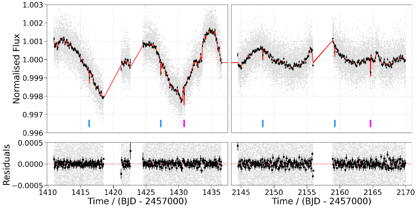
Figure 1: TESS PDCSAP lightcurve from sector 4 (left) and sector 31 (right). The 2 minute cadence data (grey) has been binned to 120 minutes (black squares) to guide the eye. The red line is the median model from the global photometric fit, described in Section 4.2, and the red shaded region (difficult to see on this scale) is the 1$\sigma$ uncertainty on the model. The blue and pink markers indicate the mid-transit times of the inner and outer planet, respectively. The lower panels show the residuals of the median model.

From the sector 4 data alone, the transiting planet search (TPS; Jenkins, 2002; Jenkins et al., 2010b, 2020) performed by the SPOC pipeline identified a single planet candidate. This planet candidate was announced as TOI 461.01 in February 2019 with an epoch of 1416.3 (BJD - 2457000) and a period of 14.5 days. When the sector 31 data became available, we performed a by-eye search of the lightcurve and realised that TOI 461.01 was actually a combination of two planetary signals. There was one multi-transiting planet candidate, with an epoch of 1416.3 (BJD - 2457000) and a period of 10.9 days, and one duotransit - a planet candidate with one transit in sector 4 and one transit in sector 31, separated by $T_{\text{diff}}\sim$ 733.8 days. When a multi-sector TPS was performed by SPOC in May 2021, it correctly identified the multi-transiting planet candidate and the ephemeris of TOI 461.01 was updated accordingly. This planet candidate passed all of the SPOC vetting tests (Twicken et al., 2018; Li et al., 2019), including the difference image centroid test, the odd-even depth test and the ghost diagnostic test, and the source of the transit signal was localised within 6.0 $\pm$ 4.2″ of HD 15906. The duotransit did not receive a TOI designation.

The TESS data contains four transits of the inner planet candidate (TOI 461.01, hereafter called HD 15906 b) and two transits of the outer planet candidate (hereafter called HD 15906 c). From the TESS data alone, the orbital period of the outer planet candidate was ambiguous. There existed a discrete set of 36 allowed period aliases, in the range 20.4 - 733.8 days (see Section 4.1), and follow-up observations were therefore required to recover the correct period.

2.2 CHEOPS Photometry

To recover the period of the outer planet candidate, we observed HD 15906 through the CHEOPS GTO programme CH_PR110048 ("Duos - Recovering long period duo-transiting planets"). Our observing strategy was informed by our analysis of the TESS data (see Section 4.1). We scheduled CHEOPS observations of the 13 highest probability period aliases ($P$ $<$ 31 days), giving highest priority to the four most probable period aliases ($P$ $<$ 22.5 days). The first and second CHEOPS visits did not reveal a transit and ruled out six period aliases in total. The third CHEOPS visit revealed a transit and uniquely confirmed a period of $\sim$ 21.6 days for HD 15906 c. A fourth CHEOPS visit, scheduled before the period had been confirmed, did not reveal a transit. We scheduled one additional observation of both HD 15906 b and c to improve radius precision and search for possible transit timing variations (TTVs). For all of our CHEOPS observations, we used an exposure time of 60 seconds with no on-board image stacking, resulting in a final lightcurve cadence of 60 seconds. A summary of our six CHEOPS observations is presented in Table 1.

Table 1: CHEOPS observations of HD 15906. See Section 4.2.1 for a description of the detrending terms.

Visit	File Key	Start Time [UTC]	Dur. / hrs	Eff. / %	Planet	Transit Observed?	Detrending Terms
1	CH_PR110048_TG005901_V0200	2021-09-21 12:41:29	8.10	71	c	no	bg, t, cos($\phi$)
2	CH_PR110048_TG006201_V0200	2021-09-29 20:02:09	8.10	74	c	no	x, y
3	CH_PR110048_TG005301_V0200	2021-09-30 19:07:09	8.10	73	c	yes	bg, x, y, t, cos(3$\phi$)
4	CH_PR110048_TG005101_V0200	2021-10-03 01:25:29	7.99	74	c	no	bg, y, t, cos(3$\phi$)
5	CH_PR110048_TG009901_V0200	2021-10-10 02:48:09	9.27	86	b	yes	bg, x, y, t, cos(2$\phi$), sin(3$\phi$)
6	CH_PR110048_TG009801_V0200	2021-11-12 22:11:30	8.39	74	c	yes	bg, y, t

Due to the fact CHEOPS is in a low-Earth orbit, with an orbital period $\sim$ 98.7 minutes, our observations suffer from interruptions caused by high levels of stray light (from the illuminated Earth limb), occultations of the target by the Earth and passage of the satellite through the South Atlantic Anomaly (SAA; Benz et al., 2021). These interruptions result in gaps in the CHEOPS lightcurves, reducing the observing efficiency (time spent collecting data divided by the duration of the visit). The efficiencies of our six visits are included in Table 1 and the inset of Figure 2 shows examples of the lightcurve gaps.

For each of our CHEOPS visits, sub-array images and lightcurves were produced by the Data Reduction Pipeline (DRP 13.1.0; Hoyer et al., 2020). The sub-array images are circular, with a diameter of 200 pixels ($\sim$ 200″), and are centred on the target star. They are calibrated and corrected for effects such as cosmic ray hits, smear trails caused by nearby stars and variations in background flux. From these images, the DRP uses aperture photometry to produce four lightcurves using circular apertures of different sizes. The DEFAULT, RINF and RSUP apertures are predefined with radii 25, 22.5 and 30 pixels respectively. The OPTIMAL aperture is selected per visit to minimise the effect of instrumental noise and contamination from nearby stars. We downloaded the CHEOPS sub-array images and DRP lightcurves from the Data & Analysis Center for Exoplanets (DACE; Buchschacher et al., 2015). Alongside the time, flux and flux error, the DRP lightcurves include a set of detrending vectors that can be used to model instrumental trends in the lightcurve. This includes the background flux, the smearing and contamination from nearby stars, the x and y centroid position of the target star and the roll angle of the satellite. CHEOPS rolls around its pointing direction once per orbit, to maintain thermal stability, and every data point has an associated roll angle between 0 and 360 degrees.

We also extracted our own lightcurves from the CHEOPS sub-array images using point-spread function (PSF) photometry. This technique is complementary to the aperture photometry performed by the DRP. We used the PSF Imagette Photometric Extraction (PIPE) package (see description in Deline et al., 2022), which was developed specifically for CHEOPS data. PIPE photometry is less sensitive to contamination from nearby stars and the effects of smear trails are removed before extracting the flux (Serrano et al., 2022b). The PIPE lightcurves contain the time, flux and flux error, as well as the same detrending vectors as the DRP lightcurves, with the exception of smearing and contamination.

We performed preliminary transit fits of the DRP and PIPE lightcurves using pycheops (Maxted et al., 2021) and found that the planet parameters obtained in each case were fully compatible. We then compared the photometric precision of the DRP and PIPE lightcurves for each CHEOPS visit. Firstly, we performed iterative outlier clipping as described in Section 2.1. Then, we calculated the MAD of each clipped lightcurve, see Table 2. We found that for four of the six visits, including all three transit observations, the PIPE lightcurve had the lowest MAD. In the other two visits, the MAD of the PIPE lightcurve was comparable to the lowest value. We therefore chose to use the PIPE photometry for our analysis.

Table 2: Mean absolute deviation (MAD) of the clipped CHEOPS lightcurves. The lightcurve with the lowest MAD for each visit is in bold.

Visit	MAD / ppm
	DEFAULT	OPTIMAL	RINF	RSUP	PIPE
1	228.8	239.8	225.2	239.2	231.3
2	210.2	275.5	220.4	221.8	208.2
3	291.9	346.0	348.4	326.3	217.4
4	236.5	289.9	258.3	260.3	247.4
5	230.3	348.9	235.3	279.8	223.6
6	211.4	237.1	227.6	214.2	209.5

To prepare the PIPE lightcurves for our analysis, we performed a series of cuts to the data. Firstly, we rejected all flagged data. PIPE assigns flags to data of lesser quality, for example due to outliers in centroid position or a large number of bad pixels in the frame. Next, we performed a cut to remove data with high background flux. Some of the CHEOPS lightcurves showed sharp spikes in the target’s flux immediately before and/or after the data gaps (see an example in the inset of Figure 2). These spikes coincide with the target star approaching the illuminated Earth limb, causing high levels of scattered light and an increase in the background flux. This can be seen in Figure 2, where we have plotted the background flux against the angle between the instrument’s line of sight (LOS) and the Earth limb for all six CHEOPS visits. Notice that not all of the observations with a small angle have a high background flux; it is only when the star approaches the Earth’s day side that there is a significant increase in scattered light. We removed all data with background flux $>$ 10 000 e^-pix^-1 because this adequately reduced the spikes in the lightcurves whilst retaining as much data as possible. After the background cut, we removed remaining outliers from the lightcurves using the same iterative MAD clipping described in Section 2.1. In total, these three cuts rejected 42/346 ($\sim$ 12%), 33/358 ($\sim$ 9%), 36/356 ($\sim$ 10%), 47/353 ($\sim$ 13%), 43/476 ($\sim$ 9%) and 31/375 ($\sim$ 8%) data points from each respective CHEOPS visit.

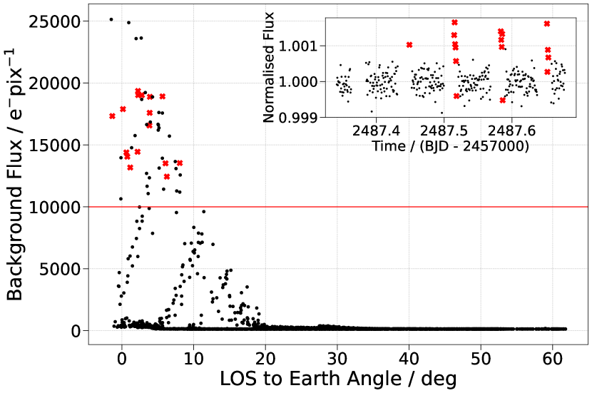
Figure 2: Background flux versus angle between the instrument’s line of sight (LOS) and the Earth limb for non-flagged data from all six CHEOPS observations. The red horizontal line represents our background cut of 10 000 e^-pix^-1 and the red crosses correspond to the data removed from CHEOPS visit 2. Inset: CHEOPS lightcurve from visit 2. Only non-flagged data is plotted and the points shown as red crosses were removed by the background cut.

Following these steps, the PIPE photometry still contained trends correlated with instrumental parameters such as background flux, centroid position and roll angle. Rather than pre-detrending the data, we chose to fit a joint transit and detrending model, see Section 4.2.

2.3 LCOGT Photometry

We conducted ground-based photometric follow-up observations of HD 15906 as part of the TESS Follow-up Observing Program (TFOP; Collins, 2019) Sub Group 1.

We used the TESS Transit Finder, a customised version of the Tapir software package (Jensen, 2013), to schedule our transit observations. We observed full predicted transit windows of HD 15906 b in Pan-STARRS $z$-short band using the Las Cumbres Observatory Global Telescope (LCOGT; Brown et al., 2013) 1.0 m network nodes at Siding Spring Observatory and McDonald Observatory on 27 August 2021 and 1 November 2021, respectively. See Table 3 for a summary of these observations. The 1.0 m telescopes are equipped with 4096 $\times$ 4096 SINISTRO cameras having an image scale of 0.389″pix^-1, resulting in a 26′ $\times$ 26′ field of view. We used an exposure time of 30 seconds and, with the full frame readout time of $\sim$ 30 seconds, the final image cadence was $\sim$ 60 seconds. The images were calibrated with the standard LCOGT BANZAI pipeline (McCully et al., 2018). The telescopes were intentionally defocused in an attempt to improve photometric precision, resulting in a typical HD 15906 full width half maximum (FWHM) of 6.5″. Differential photometric data were extracted using AstroImageJ (Collins et al., 2017). We used a circular photometric aperture with radius 9.3″ to exclude all flux from the nearest known Gaia Data Release 3 stars (Gaia DR3; Gaia Collaboration et al., 2016, 2022). A transit-like event was detected in both LCOGT lightcurves and they were included in the analysis described in Section 4.2.

Table 3: LCOGT observations of HD 15906 b. See Section 4.2.2 for a description of the detrending terms.

Visit	Observatory	Start Time [UTC]	Dur. / hrs	Detrending Terms
1	Siding Spring	2021-08-27 13:47:07	5.7	airmass, FWHM
2	McDonald	2021-11-01 03:36:18	3.8	airmass, FWHM

2.4 WASP Photometry

HD 15906 was observed 38 740 times by the Wide Angle Search for Planets at the South African Astronomical Observatory (WASP-South; Pollacco et al., 2006) between 19 August 2008 and 19 December 2014. The photometry was extracted and detrended for systematic effects following the methods described in Collier Cameron et al. (2006). Based upon a visual inspection of the lightcurve, we removed data with a normalised flux greater than 1.07 or less than 0.93 and we removed data with a relative flux error greater than 0.03. These cuts removed 5 231/38 740 ($\sim$ 14%) data points and the resulting lightcurve is shown in Figure 3. With an average flux error of $\sim$ 9 ppt, we do not detect the transits of HD 15906 b or c in the WASP data. Furthermore, there were no additional transits detected in the lightcurve. Thanks to the long baseline, the WASP photometry is used to estimate the stellar rotation period (see Section 3.3).

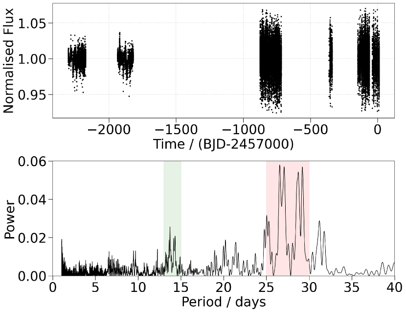
Figure 3: Archival WASP photometry. Upper: Normalised WASP lightcurve spanning more than 6 years. Lower: GLS periodogram of the WASP lightcurve. The strongest peaks are in the range 25-30 days (red highlight), followed by 13-15 days (green highlight).

2.5 HARPS Spectroscopy

The High Accuracy Radial velocity Planet Searcher (HARPS; Mayor et al., 2003) is a high-resolution (R = 115 000) fibre-fed spectrograph installed on the 3.6 m telescope at the European Southern Observatory (ESO) in La Silla, Chile. It has been operational since 2003 and the optical fibres were upgraded in 2015, leading to an offset in the measured radial velocities (RVs) (Lo Curto et al., 2015).

HARPS observed HD 15906 18 times between 3 November 2003 and 9 February 2018. There were 15 observations taken before the fibre upgrade and 3 observations taken after the upgrade. The exposure times of the observations ranged from 358 to 900 seconds and the average SNR at 550 nm was 53.7. The data spans $\sim$ 5212 days, with an average separation of $\sim$ 307 days between each observation. The HARPS spectra are publicly available on the ESO Science Archive Facility.

For our analysis of the HD 15906 system, we used the RVs presented in Trifonov et al. (2020). Specifically, we used the columns ‘RV_mlc_nzp’ and ‘e_RV_mlc_nzp’ for the RV and RV error, respectively. These RVs were extracted by the SpEctrum Radial Velocity AnaLyser (SERVAL; Zechmeister et al., 2018) pipeline, where the extraction was done independently before and after the fibre upgrade and a correction was made for the nightly zero-point. The data have a root mean square (RMS) of 10.70 ms^-1 and the average RV uncertainty is 1.51 ms^-1. We present these RVs in Table 4.

Table 4: HARPS and FIES RVs of HD 15906.

Time / BJD	RV / ms-1	RV Error / ms-1	Instrument
2452946.74714	-2.799	2.005	HARPS
2453315.66562	10.217	1.243	HARPS
2453316.79132	3.188	2.672	HARPS
2453321.79052	-7.562	1.354	HARPS
2454390.73395	-3.929	1.621	HARPS
2454438.60542	10.151	1.369	HARPS
2454752.74485	11.626	1.375	HARPS
2455217.57723	4.607	1.662	HARPS
2455491.79108	15.727	1.631	HARPS
2455876.61897	-9.996	1.475	HARPS
2456161.82258	-0.028	1.137	HARPS
2456169.84113	-11.997	1.422	HARPS
2456233.78781	-10.516	1.116	HARPS
2456271.65665	-1.351	1.135	HARPS
2456309.54995	0.427	1.614	HARPS
2457349.78566	-29.043	2.260	HARPS
2457354.71407	11.282	1.051	HARPS
2458158.55270	-5.683	1.121	HARPS
2458742.62217	2.65	4.90	FIES
2458745.71138	0.00	5.32	FIES
2458751.64001	-8.37	14.61	FIES
2458753.70368	-13.85	4.65	FIES
2458757.57125	11.98	4.64	FIES
2458765.57899	3.41	3.27	FIES
2458768.66127	-3.25	5.16	FIES

2.6 FIES Spectroscopy

As part of TFOP, we observed HD 15906 seven times using the FIbre-fed Échelle Spectrograph (FIES; Telting et al., 2014) at the Nordic Optical Telescope (NOT; Djupvik & Andersen, 2010) between 15 September 2019 and 12 October 2019. For each observation, we used the high-resolution fibre (R $\sim$ 67 000) and an exposure time of 1800 seconds. We extracted the spectra and derived multi-order RVs following Buchhave et al. (2010). The SNR per resolution element at 550 nm ranges between 20 and 105 with a median of 97. The RMS of the RV data is 7.88 ms^-1 and the average uncertainty is 6.08 ms^-1. These FIES RVs are included in Table 4.

3 Stellar Characterisation

3.1 Atmospheric Properties

As described in Section 2.5, HD 15906 was observed by HARPS 18 times between 2003 and 2018, with 15 observations made before the 2015 fibre upgrade. We retrieved the 15 pre-upgrade HARPS spectra from the ESO Science Archive Facility and co-added them to create a single master spectrum. This was used to perform the following spectroscopic analyses.

We performed an equivalent width (EW) analysis using ARES+MOOG to derive the stellar atmospheric parameters ($T_{\mathrm{eff}}$, $\log g$, microturbulence, [Fe/H]). We followed the same methodology described in Santos et al. (2013); Sousa (2014); Sousa et al. (2021). We used the latest version of ARES (Sousa et al., 2007, 2015) to measure the EWs of the iron lines in the master HARPS spectrum. We used a minimisation process to find ionisation and excitation equilibrium and converge to the best set of spectroscopic parameters. The iron abundances were computed using a grid of Kurucz model atmospheres (Kurucz, 1993) and the radiative transfer code MOOG (Sneden, 1973). We also derived a more accurate trigonometric surface gravity using recent Gaia data following the same procedure as described in Sousa et al. (2021). The quoted errors for $T_{\mathrm{eff}}$, $\log g$ and [Fe/H] are “accuracy” errors, that is they have been corrected for systematics following the discussion presented in Section 3.1 of Sousa et al. (2011). The final spectroscopic parameters and their errors are included in Table 5 and we find that HD 15906 is a K-dwarf.

We also performed an independent spectral synthesis with SME version 5.2.2 (Spectroscopy Made Easy; Valenti & Piskunov, 1996; Piskunov & Valenti, 2017). A detailed description of the modelling can be found in Persson et al. (2018). We used the ATLAS12 stellar atmosphere grid (Kurucz, 2013) and atomic and molecular line data from VALD (Vienna Atomic Line Database; Ryabchikova et al., 2015). The macro- and micro-turbulent velocities were held fixed to 1.5 kms^-1 and 0.5 kms^-1, respectively. The resulting $T_{\mathrm{eff}}$, $\log g$ and abundances were in excellent agreement with the ARES+MOOG analysis. We additionally derived the projected rotational velocity, $v\sin i_{\star}$ = 2.7 $\pm$ 0.7 kms^-1.

Table 5: Stellar properties of HD 15906.

HD 15906
Alternative Identifiers
TOI	461
TIC	4646810
TYC	5282-297-1
2MASS	J02330530-1021062
Gaia DR3	5175239363214344960
Parameter	Value	Source
Astrometric Properties
RA (J2016; hh:mm:ss.ss)	02:33:05.09	1
Dec (J2016; dd:mm:ss.ss)	-10:21:07.89	1
$\mu_{\alpha}$ / mas yr-1	-172.92 $\pm$ 0.02	1
$\mu_{\delta}$ / mas yr-1	-92.22 $\pm$ 0.02	1
RV / kms-1	-3.64 $\pm$ 0.25	1
Parallax / mas	21.834 $\pm$ 0.019	1*
Distance / pc	45.80 $\pm$ 0.04	6; inverse parallax
U / kms-1	37.87 $\pm$ 0.20	6
V / kms-1	9.56 $\pm$ 0.01	6
W / kms-1	-17.25 $\pm$ 0.35	6
Photometric Properties
G / mag	9.484 $\pm$ 0.003	1
GBP / mag	9.999 $\pm$ 0.003	1
GRP / mag	8.817 $\pm$ 0.004	1
TESS / mag	8.872 $\pm$ 0.006	2
V / mag	9.76 $\pm$ 0.03	3
B / mag	10.79 $\pm$ 0.06	3
J / mag	8.035 $\pm$ 0.018	4
H / mag	7.557 $\pm$ 0.031	4
K / mag	7.459 $\pm$ 0.023	4
W1 / mag	7.345 $\pm$ 0.032	5
W2 / mag	7.459 $\pm$ 0.020	5
Bulk Properties
$T_{\mathrm{eff}}$ / K	4757 $\pm$ 89	6; ARES+MOOG
$\log g$ / cms-2	4.49 $\pm$ 0.05	6; ARES+MOOG
[Fe/H] / dex	0.02 $\pm$ 0.04	6; ARES+MOOG
$v\sin i_{\star}$ / kms-1	2.7 $\pm$ 0.7	6; SME
$\log R^{\prime}_{\mathrm{HK}}$	-4.694 $\pm$ 0.065	6; HARPS spectra
E(B - V)	0.023 $\pm$ 0.018	6; IRFM
$R_{\star}$ / $R_{\odot}$	0.762 $\pm$ 0.005	6; IRFM
$M_{\star}$ / $M_{\odot}$	0.790${}_{-0.036}^{+0.020}$	6; isochrones
$\rho_{\star}$ / $\rho_{\odot}$	1.79 $\pm$ 0.07	6; from $R_{\star}$ and $M_{\star}$
$\rho_{\star}$ / gcm-3	2.52 $\pm$ 0.10	6; from $R_{\star}$ and $M_{\star}$
$L_{\star}$ / $L_{\odot}$	0.27 $\pm$ 0.02	6; from $R_{\star}$ and $T_{\mathrm{eff}}$

References: 1 - Gaia DR3 (Gaia Collaboration et al., 2022). 2 - TESS Input Catalog Version 8 (TICv8; Stassun et al., 2019). 3 - Tycho-2 (Høg et al., 2000). 4 - 2MASS (Skrutskie et al., 2006). 5 - WISE (Wright et al., 2010). 6 - this work, see Section 3. *Gaia DR3 parallax corrected according to Lindegren et al. (2021).

3.2 Stellar Mass and Radius

We determined the stellar radius, $R_{\star}$, of HD 15906 from the stellar angular diameter and the offset corrected Gaia DR3 parallax (Lindegren et al., 2021) using a Markov-Chain Monte Carlo Infrared Flux Method (MCMC IRFM; Blackwell & Shallis, 1977; Schanche et al., 2020). We used the stellar spectral parameters as priors to construct model spectral energy distributions (SEDs) using atmospheric models from stellar catalogues. From this, we derived the stellar bolometric flux and angular diameter by comparing synthetic photometry, computed by convolving the model SEDs over broadband bandpasses of interest, to the observed data taken from the most recent data releases for the following bandpasses; Gaia G, G_BP, and G_RP, Two Micron All-Sky Survey (2MASS) J, H, and K, and Wide-field Infrared Survey Explorer (WISE) W1 and W2 (Skrutskie et al., 2006; Wright et al., 2010; Gaia Collaboration et al., 2022). To account for systematic model uncertainties in our stellar radius error, we used stellar atmospheric models taken from a range of ATLAS catalogues (Kurucz, 1993; Castelli & Kurucz, 2003) and combined them in a Bayesian modelling averaging framework. Within the MCMC IRFM we attenuated the SED to correct for potential extinction and report the determined E(B-V) in Table 5. We combined the retrieved angular diameter with the offset-corrected Gaia DR3 parallax and found $R_{\star}$ = 0.762 $\pm$ 0.005 $R_{\odot}$.

We then determined the stellar mass, $M_{\star}$, by inputting $T_{\mathrm{eff}}$, [Fe/H], and $R_{\star}$ into two different stellar evolutionary models, PARSEC v1.2S (PAdova and TRieste Stellar Evolutionary Code; Marigo et al., 2017) and CLES (Code Liégeois d’Évolution Stellaire; Scuflaire et al., 2008). We employed the isochrone placement algorithm (Bonfanti et al., 2015, 2016) to interpolate the input parameters within pre-computed grids of PARSEC isochrones and tracks and we retrieved a first estimate of the stellar mass, $M_{\star\mathrm{,PD}}$ = 0.772 $\pm$ 0.037 $M_{\odot}$. A second estimate was computed through the CLES code, which builds the best-fit evolutionary track of the star by applying the Levenberg-Marquadt minimisation scheme (e.g., Salmon et al., 2021) and we found $M_{\star\mathrm{,LG}}$ = 0.797 $\pm$ 0.014 $M_{\odot}$. To account for model-related uncertainties, we added in quadrature an uncertainty of 4% to the mass estimates obtained from each set of models (see Bonfanti et al., 2021). We note that the two outcomes are well within 1$\sigma$. We also checked their mutual consistency through the $\chi^{2}$-based criterion broadly presented in Bonfanti et al. (2021) and obtained a p-value = 0.49, which is greater than the normally adopted significance level of 0.05, as expected. For each mass estimate, we built the corresponding Gaussian probability density function, as described in Bonfanti et al. (2021), and we combined them to obtain a final mass value of $M_{\star}$ = 0.790${}_{-0.036}^{+0.020}M_{\odot}$, as presented in Table 5.

3.3 Stellar Age

The isochrone fitting described in Section 3.2 also provided an estimate of the stellar age. However, the stellar mass is sufficiently low that the slow evolutionary speed of the star along its tracks led to an uninformative age of 6.8${}_{-6.3}^{+6.9}$ Gyr. To try and constrain the stellar age more precisely, we used gyrochronology, empirical $\log R^{\prime}_{\mathrm{HK}}$ relations and kinematics.

For the gyrochronology, we first estimate the stellar rotation period, P_rot. The TESS photometry (Figure 1) shows flux modulation, likely caused by stellar activity, that can be used to do this. We conducted a generalised Lomb-Scargle (GLS; Lomb, 1976; Scargle, 1982; Zechmeister & Kürster, 2009) analysis on the TESS SAP and PDCSAP photometry and found strong peaks at 11-12 days and 25-27 days. However, this analysis is adversely affected by the short $\sim$ 27 day baseline of the TESS lightcurves. The archival WASP photometry has a much longer baseline that can be used to derive an independent estimate of the stellar rotation period. We performed a GLS analysis on the WASP lightcurve, the results of which are shown in Figure 3. The strongest peaks are in the range 25-30 days, with the maximum power at 26.6 days corresponding to a best-fit photometric amplitude of $\sim$ 4 ppt. The next strongest peaks are in the range 13-15 days, with a maximum power at 13.7 days and an amplitude of $\sim$ 3 ppt. This shorter rotation period is supported by our value of $v\sin i_{\star}$. Assuming $\sin i_{\star}$ = 1 and using the stellar radius in Table 5 leads to an upper limit of the rotation period, P_rot = 14.3 $\pm$ 3.7 days. Finally, from a GLS analysis of the HARPS and FIES RVs (see Section 4.4), we found that the peak power was at 12.27 days with a false alarm probability (FAP) of less than 1%. It’s possible that this corresponds to the stellar rotation period, however, due to the very sparse sampling of the RVs, this value is unreliable. The stellar rotation period remains somewhat ambiguous, but the evidence favours a value in the range 11-15 days. Using the gyrochronological relations of Barnes (2007) and (B-V) from Table 5, these P_rot values yield a stellar age in the range 0.29-0.52 Gyr. We note that the longer P_rot values (25-30 days) would translate to an age of 1.39-1.97 Gyr. However, more recent studies have shown that the relations of Barnes (2007) might lead to an incorrect age estimate for low-mass stars because they do not account for the stalling period during spin-down (e.g., Curtis et al., 2020). Based upon a sample of benchmark stellar clusters, a rotation period of 11-15 days for a star with a similar effective temperature as HD 15906 is consistent with an age up to $\sim$ 1 Gyr.

Next, we computed values of $\log R^{\prime}_{\mathrm{HK}}$ from each of the 18 HARPS spectra using ACTIN (Gomes da Silva et al., 2018) to extract the Ca ii index and following the method described in Gomes da Silva et al. (2021) for the $\log R^{\prime}_{\mathrm{HK}}$ calibration. We found an average value of -4.694 $\pm$ 0.065 and, using the empirical relations of Mamajek & Hillenbrand (2008), this converts into a stellar age of 1.9 $\pm$ 0.7 Gyr.

Finally, we computed the kinematic age using the method developed in Almeida-Fernandes & Rocha-Pinto (2018) and the Galactic $UVW$ velocities that we determined from the Gaia DR3 proper motions, offset-corrected parallax (Lindegren et al., 2021), and stellar RV, using the method outlined in Johnson & Soderblom (1987). We found a stellar age of 1.9${}^{+6.0}_{-0.7}$ Gyr, favouring an older star.

In Figure 4, we present a comparison of the age estimates derived by our various methods. The age estimates derived from $\log R^{\prime}_{\mathrm{HK}}$ and kinematics are consistent and they are in agreement with the gyrochronological age implied by a rotation period of 25-30 days. The favoured rotation period of 11-15 days yields a much younger age, however we reiterate that gyrochronology is not necessarily accurate for low-mass stars. We conclude that the stellar age is ambiguous based on the current data.

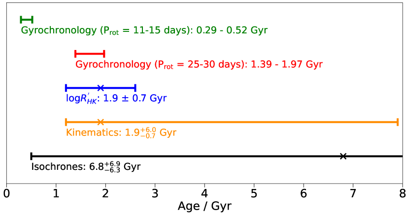
Figure 4: A comparison of stellar age estimates obtained from isochrone fitting, $\log R^{\prime}_{\mathrm{HK}}$ relations, kinematics and gyrochronology.

4 Analysis

4.1 TESS Only Analysis

Before pursuing CHEOPS follow-up observations of HD 15906, we used MonoTools (Osborn, 2022) to perform an analysis of the TESS data. MonoTools is designed for the analysis of planets with unknown periods, including duotransits. It can be used to derive the allowed period aliases and their corresponding probabilities, crucial for scheduling follow-up observations.

We built a MonoTools model using the stellar parameters presented in Table 5, one periodic planet and one duotransit. We defined initial guesses for transit depth, duration, and mid-transit time for the two planets using a visual inspection of the TESS lightcurve. Since this is a multiplanet transiting system, we selected the eccentricity distribution from Van Eylen & Albrecht (2015). We also included a Gaussian Process (GP; Rasmussen & Williams, 2006; Gibson, 2014) with a simple harmonic oscillator (SHO) kernel from celerite (Foreman-Mackey et al., 2017) to model the correlated noise in the lightcurve. We sampled the posterior probability distribution using the No-U-Turn Sampler (NUTS; Hoffman & Gelman, 2014), a variant of Hamiltonian Monte Carlo, implemented via pyMC3 (Salvatier et al., 2016).

We found that the duotransit, HD 15906 c, had 36 possible period aliases, with a minimum value, P${}_{\text{min}}$, of 20.384 days. The probability of each period alias is shown in Figure 5. These results were used to schedule our CHEOPS follow-up observations, from which we successfully determined the true period of planet c to be $\sim$ 21.6 days (see Section 2.2).

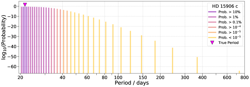
Figure 5: From the TESS data alone, HD 15906 c was a duotransit with 36 possible period aliases. This plot shows these aliases and their corresponding probabilities, derived using MonoTools. The true period, as determined by CHEOPS follow-up observations, had the highest probability.

4.2 Global Photometric Analysis

Once we had confirmed the true period of HD 15906 c with CHEOPS, we performed a joint fit of the TESS, CHEOPS and LCOGT photometric data using juliet(Espinoza et al., 2019). This package combines transit models from batman (Kreidberg, 2015) with the option to include linear models and GPs to model instrumental noise and stellar variability. We created a model consisting of two transiting planets, using the following parameterisation:

• Orbital period, $P$, and mid-transit time, $T_{0}$, for both planets. We set broad uniform priors on $P$ and $T_{0}$ from a visual inspection of the TESS and CHEOPS lightcurves.

• Planet-to-star radius ratio, $p$ = R${}_{\text{P}}$ / R_⋆, and impact parameter, $b$, for both planets. We set uniform priors to allow exploration of all physically plausible solutions.

• Eccentricity, $e$, and argument of periastron, $\omega$, for both planets. We used the eccentricity prior from Van Eylen et al. (2019) for systems with multiple transiting planets – the positive half of a Gaussian with $\mu$ = 0 and $\sigma$ = 0.083. We used a uniform prior for $\omega$, covering the full range of possible values. We decided to fit for eccentricity, rather than assuming a circular orbit, to ensure that the uncertainties on the other fitted parameters were not underestimated. We note that we repeated our final global photometric fit assuming a circular orbit, with $e$ fixed to zero and $\omega$ fixed to 90 degrees, and all of the fitted planet parameters were consistent within 1.2$\sigma$.

• Stellar density, $\rho_{\star}$. Using Kepler’s third law, this can be combined with $P$ to derive a value of $a/R_{\star}$ for each planet. This is preferred to fitting for $a/R_{\star}$ directly; not only does it reduce the number of fitted parameters, but it also ensures a consistent value of $\rho_{\star}$. We defined a normal prior on $\rho_{\star}$ using the values of $R_{\star}$ and $M_{\star}$ presented in Table 5.

• Quadratic limb darkening parameters, $q1$ and $q2$, for each instrument. We used the Kipping (2013) parameterisation of the quadratic limb darkening law and defined normal priors on $q1$ and $q2$ for each instrument. The mean was computed by interpolating tables of quadratic limb darkening coefficients (Claret, 2017, 2021; Claret & Bloemen, 2011), based on the stellar parameters presented in Table 5, and a standard deviation of 0.1 was used in all cases.

In addition to the transit models, we used linear models to detrend CHEOPS and LCOGT against instrumental systematics, see Sections 4.2.1 and 4.2.2. We treated each CHEOPS and LCOGT observation independently for the sake of this detrending. We also included a GP to model the variability in the TESS lightcurve, see Section 4.2.3. For each instrument, we included a jitter term to account for white noise and a relative flux offset term. We fixed the dilution factor to 1 due to the lack of any bright contaminating sources (see Section 6.4). We used the dynesty package to sample the posterior probability of this model with static nested sampling, using 300 live points and stopping when the difference between the evidence and the estimated remaining evidence was less than 0.01 (Speagle, 2020). For a full list of the parameters and priors used in our global fit see Appendix A and for the results of our modelling see Section 5.1.

4.2.1 CHEOPS Detrending

The CHEOPS lightcurves contain trends that are correlated with instrumental parameters such as background flux (bg) and centroid position (x, y). There are also periodic noise features that repeat once per CHEOPS orbit due to the satellite rolling around its pointing direction. Detrending the lightcurve against the sine or cosine of the roll angle ($\phi$) can remove these periodic instrumental effects.

The CHEOPS lightcurves also include stellar variability. From the TESS LC we know that HD 15906 shows stellar variability (see Figure 1). On the shorter timescale of a CHEOPS visit ($\sim$ 8.3 hours), this stellar variability can be modelled with a linear trend in time (t).

We included linear models in our global fit to account for these instrumental trends and stellar variability. However, for each CHEOPS observation, it was important to only select the relevant detrending parameters. To do this we used the pycheops package (Maxted et al., 2021) and the method described in Swayne et al. (2021). Briefly, we defined 10 detrending parameters: x, y, t, bg, cos($\phi$), sin($\phi$), cos(2$\phi$), sin(2$\phi$), cos(3$\phi$) and sin(3$\phi$). For each CHEOPS visit, we took the clipped lightcurve (see Section 2.2) and did an initial fit of a transit model with no detrending. We defined broad uniform priors on the transit parameters based on a visual inspection of the TESS and CHEOPS data. We used the RMS of the residuals from this initial fit to define normal priors on the detrending parameters, with $\mu$ = 0 and $\sigma$ = RMS. We added the 10 detrending parameters to the fit one-by-one, selecting the parameter with the lowest Bayes factor at each step. When there were no remaining parameters with Bayes factor $<$ 1, we stopped adding detrending parameters. In order to remove strongly correlated parameters, if any of the selected detrending parameters had a Bayes factor $>$ 1, we removed the parameter with the largest Bayes factor until no more parameters with Bayes factor $>$ 1 remained. The selected detrending parameters for each CHEOPS visit are included in Table 1.

4.2.2 LCOGT Detrending

We used AstroImageJ to select the relevant detrending vectors for each LCOGT observation by jointly fitting a transit model and linear combinations of zero, one, or two detrending parameters from the available detrending vectors: airmass, time, sky background, FWHM, x-centroid, y-centroid, total comparison star counts, humidity and exposure time. The best zero, one, or two detrending vectors were retained if they reduced the Bayesian information criterion (BIC) for a fit by at least two per detrending parameter. We found that the airmass plus FWHM detrending pair provided the best improvement to the lightcurve fit for both LCOGT observations. We therefore included linear models for airmass and FWHM for each LCOGT observation in our global fit.

4.2.3 TESS Detrending

The TESS lightcurves contain correlated noise, including stellar variability and residual instrumental systematics, that we model with a GP. We initially modelled sector 4 and sector 31 jointly, using a GP with an approximate Matérn-3/2 (M32) kernel implemented via celerite (Foreman-Mackey et al., 2017). Upon a visual inspection of the results from this fit, we noticed that the TESS residuals contained a sinusoidal-like trend. We ran a GLS analysis on the TESS residuals, treating the sector 4 and sector 31 data separately, and the resulting periodograms are presented in Figure 6. We found a significant periodic signal in the TESS sector 4 residuals, with a period of 0.22004 days and a FAP of 6.0 x 10^-11. This signal is persistent throughout the whole of sector 4 and the best-fit sinusoidal model has an amplitude of $\sim$ 57 ppm. There was no corresponding detection in the TESS sector 31, CHEOPS or LCOGT residuals. The periodic signal is present in the TESS lightcurve itself, it was not introduced as a result of our detrending, and we discuss its origin in Section 7.1.

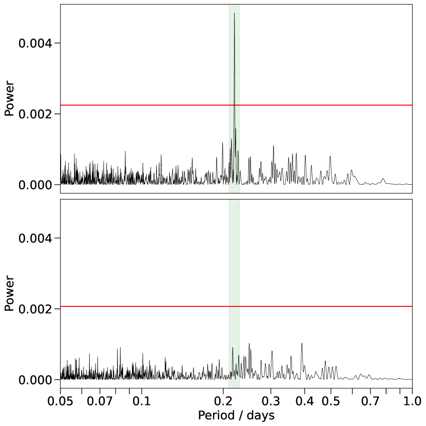
Figure 6: GLS periodogram of the TESS residuals from a global photometric fit using a GP with a Matérn-3/2 kernel to jointly model TESS sector 4 and sector 31. Upper: GLS periodogram of sector 4 residuals. Lower: GLS periodogram of sector 31 residuals. The horizontal red line is the 1% false alarm probability level in each case. The significant peak at 0.22004 days in the sector 4 residuals (highlighted in green) is not present in the sector 31 residuals.

A half-cycle of the periodic signal is a similar duration to the transits and it was therefore important to check if it was affecting the fitted planet parameters. We therefore performed two additional fits, changing only the TESS detrending to account for this periodic signal. We made a custom GP kernel by adding together the M32 and SHO kernels from celerite. The M32 kernel was intended to capture the long-term variability and the SHO kernel was used to capture the short-term quasi-sinusoidal noise. We defined a normal prior on the natural frequency of the SHO kernel, $\omega_{0}$, using the peak and its width from the periodogram analysis. We performed one fit where we jointly modelled the sector 4 and sector 31 data with this kernel and we also performed a fit where we decoupled the sector 4 and sector 31 data. We used the M32 plus SHO kernel for sector 4 and the M32 kernel for sector 31, motivated by the fact we only detect the periodic trend in sector 4. After performing these two fits, we checked for periodicity in the TESS sector 4 residuals. In both cases, the peak of the periodogram was still at 0.22004 days but with a FAP greater than 68%. This confirms that the SHO kernel adequately removes the periodic trend from the sector 4 TESS data.

We checked the consistency of the fitted planet parameters between the three fits. The majority of the fitted planet parameters were consistent between all three of the fits within 1$\sigma$ and the remaining parameters were consistent within 2$\sigma$, except for the argument of periastron of the outer planet. There was a disagreement greater than 3$\sigma$ between the values from the joint M32 fit and the decoupled fit. Constraining eccentricity and the argument of periastron is challenging with photometry alone and we remind the reader that we only included them in our fit to ensure that the uncertainties on the other fitted parameters were not underestimated. We conclude that the fitted planet parameters are not significantly affected by the presence of the periodic signal in TESS sector 4.

We also compared the Bayes evidence (dlnZ) of the three fits (Table 6). We found a decisive preference for both of the fits incorporating the SHO kernel over the original fit (Kass & Raftery, 1995). The joint M32 plus SHO fit had the highest evidence, preferred over the original joint M32 fit with dlnZ = 106.8, and the decoupled fit of sector 4 and 31 was preferred over the original joint M32 fit with dlnZ = 89.2.

Table 6: Comparison of the Bayes evidence from three global photometric fits, where only the TESS detrending was varied. The difference in Bayes evidence (dlnZ) between each fit and the original joint Matérn-3/2 (M32) fit is quoted, indicating a decisive preference for the fits incorporating a simple harmonic oscillator (SHO) kernel (Kass & Raftery, 1995).

TESS Detrending Model	dlnZ
Joint M32 + SHO GP	+106.8
Sector 4 M32 + SHO GP, Sector 31 M32 GP	+89.2
Joint M32 GP	0.0

Despite the fact the evidence favoured the model with the M32 plus SHO kernel jointly fit to sectors 4 and 31, the model where we decoupled sector 4 and sector 31 is more physically motivated. This is because we only detected the periodic signal in sector 4. We therefore chose the decoupled fit as our final global photometric fit and we present the results in Section 5.1.

We performed one last test to assess the dependence of our results on our chosen detrending model – we repeated the decoupled fit, replacing the M32 kernels with SHO kernels. For sector 4, we used an SHO kernel for the short-term quasi-periodic signal summed with a second SHO kernel for the longer-term variability. For sector 31, we used a single SHO kernel. All of the fitted planet parameters were fully consistent with our final results (see Table 7) within 1$\sigma$, except for the eccentricity of the inner planet which was consistent within 2.3$\sigma$. We conclude that our results are not significantly influenced by the choice of GP kernel.

4.3 Transit Timing Variation Analysis

From the global photometric analysis, we found that HD 15906 b and c orbit close to a 2:1 period commensurability ($P_{c}$/$P_{b}$ = 1.976), an indication that the planets might be in mean motion resonance (MMR). Planets in or near a low-order period commensurability have amongst the largest amplitude TTVs (e.g., Veras et al., 2011; Agol & Fabrycky, 2018), so we therefore checked for TTVs in the HD 15906 system.

juliet can incorporate TTVs into a photometric model, however, it expects that each instrument contains at least one transit of all the planets being fit. This is not true in our case – none of the CHEOPS or LCOGT observations contain a transit of both planets. We therefore had to perform a separate TTV fit for each planet. When fitting the inner planet, we included the TESS data, CHEOPS visit 5 and both LCOGT visits. For the outer planet, we included the TESS data and CHEOPS visits 3 and 6. In total, we had seven transits of the inner planet and four transits of the outer planet.

For the fit of each planet, we used a model consisting of one transiting planet and the same detrending as described in Section 4.2. The only difference in the transit model was that we fit for the individual transit times instead of $P$ and $T_{0}$. We set a uniform prior of width 0.1 days on each transit time based upon a visual inspection of the data. All other priors were unchanged from the global photometric analysis and we used dynesty to sample the posterior of the model with nested sampling. Our results are presented in Section 5.2.

4.4 Radial Velocity Analysis

From HARPS and FIES, we have 25 sparsely sampled RV data points that show a relatively large scatter, see Figure 7. We ran a GLS periodogram on the RV data and found no significant peaks at the planetary periods. The strongest peak was at 12.27 days and the best-fit sinusoid with this period had an amplitude of $\sim$ 10 ms^-1. It is possible that this signal is caused by stellar activity, but with such large gaps between each observation, the short-period peaks in the GLS periodogram are unreliable. We removed the best-fit sinusoid from the RV data and re-ran the GLS periodogram – no additional peaks emerged.

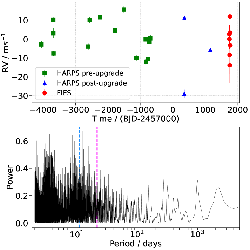
Figure 7: Upper: HD 15906 RV time-series, highlighting the sparsity of the data. HARPS data taken before/after the 2015 fibre upgrade is plotted (green squares/blue triangles) alongside the FIES data (red circles). Lower: GLS periodogram of the HARPS and FIES RV data. The photometrically derived orbital periods of the two planets, see Table 7, are indicated by the blue and pink vertical dashed lines and the red horizontal line represents the 1% false alarm probability level. There are no significant peaks at the planet periods and the strongest peak is at 12.27 days.

To search for the planetary signals, we performed a series of fits to the HARPS and FIES RV data using juliet. For our first fit, we assumed that there were no planets in the system and we fit only for an offset and a white noise term for each instrument. We used a uniform prior for the offset, in the range -20 to 20 ms^-1, and a log-uniform prior for the white noise term, in the range 0.01 to 20 ms^-1. The HARPS data from before and after the fibre upgrade had to be treated as two independent instruments. However, we only had 3 data points from post-upgrade which was insufficient to constrain the instrumental parameters. We therefore excluded the 3 post-upgrade HARPS data points from our fits and we used dynesty to sample the posterior of the model.

We then added planets to our model. We performed one fit with only the inner planet, one fit with only the outer planet and finally a fit with both planets. We used a Keplerian for each planet, generated via RadVel (Fulton et al., 2018), with the following parameterisation:

• Orbital period, $P$, and mid-transit time, $T_{0}$. We fixed these to the solution from the global photometric fit (Table 7).

• Eccentricity, $e$, and argument of periastron, $\omega$. For simplicity, we fixed eccentricity to zero and $\omega$ to 90 degrees.

• Semi-amplitude, $K$. We used a broad uniform prior to allow exploration of the range 0 to 20 ms^-1.

Finally, we took the model with both planets and added a GP with a quasi-periodic kernel (Foreman-Mackey et al., 2017) to account for the stellar activity. This kernel is described by four hyperparameters: the amplitude, period, an additive factor impacting the amplitude and the scale of the exponential component. For the amplitude we used a uniform prior in the range 0 to 20 ms^-1 and for the period we defined a normal prior using the peak from the periodogram analysis ($\mu$ = 12.27 days, $\sigma$ = 0.1 days). The other two hyperparameters were allowed to vary uniformly over a broad range. With such a small number of sparsely sampled RVs, the GP was unlikely to yield a meaningful result but we chose to include it for completeness. The results of our RV modelling are presented in Section 5.3.

We note that we also tried a joint fit of the TESS, CHEOPS and LCOGT photometric data with the HARPS and FIES RV data using juliet. The photometric model was identical to that presented in Section 4.2 and we used the RV model with two planets but no GP. However, due to the small number of sparse RVs, the fitted planet parameters were adversely affected compared to those from the global photometric model. Therefore, we decided to present independent analyses of the photometry and RVs in this paper.

5 Results

5.1 Global Photometric Results

In Section 4.2, we described our joint fit of the TESS, CHEOPS and LCOGT photometry and we present the resulting fitted planetary parameters in Table 7. We also include the following derived planetary parameters: transit depth ($\delta$ = (R${}_{\text{P}}$ / R_⋆)²), planet radius (R${}_{\text{P}}$), semi-major axis (a), orbital inclination (i), total transit duration (T${}_{\text{dur}}$), insolation flux (S${}_{\text{P}}$) and equilibrium temperature assuming zero bond albedo and full day-night heat redistribution (T${}_{\text{eq}}$).

Table 7: Fitted and derived parameters for HD 15906 b and c from the global photometric fit presented in Section 4.2.

Parameter	HD 15906 b	HD 15906 c
Fitted Parameters
$P$ / days	10.924709 $\pm$ 0.000032	21.583298${}^{+0.000052}_{-0.000055}$
$T_{0}$ / (BJD - 2457000)	1416.3453${}^{+0.0034}_{-0.0028}$	1430.8296${}^{+0.0027}_{-0.0025}$
R${}_{\text{P}}$ / R⋆	0.027 $\pm$ 0.001	0.035 $\pm$ 0.001
$b$	0.86 $\pm$ 0.03	0.90$\pm$ 0.01
$e$	0.11${}^{+0.04}_{-0.03}$	0.04 $\pm$ 0.01
$\omega$ / deg	160.5${}^{+76.9}_{-75.7}$	247.9${}^{+38.8}_{-45.4}$
$\rho_{\star}$ / kgm-3	2583.24${}^{+68.01}_{-57.80}$
Derived Parameters
$\delta$ / ppm	729${}^{+54}_{-53}$	1243${}^{+54}_{-51}$
R${}_{\text{P}}$ / R⊕	2.24 $\pm$ 0.08	2.93${}^{+0.07}_{-0.06}$
a / R⋆	25.35${}^{+0.22}_{-0.19}$	39.92${}^{+0.35}_{-0.30}$
a / AU	0.090 $\pm$ 0.001	0.141${}^{+0.002}_{-0.001}$
i / deg	87.98${}^{+0.16}_{-0.12}$	88.75${}^{+0.02}_{-0.03}$
T${}_{\text{dur}}$ / hrs	1.80${}^{+0.07}_{-0.08}$	2.19 $\pm$ 0.03
S${}_{\text{P}}$ / S⊕	33.14${}^{+2.60}_{-2.45}$	13.37${}^{+1.05}_{-0.99}$
T${}_{\text{eq}}$ / K	668 $\pm$ 13	532 $\pm$ 10

Figures 1, 8 and 9 show the TESS, CHEOPS and LCOGT data alongside the global photometric model. Figure 10 shows the detrended TESS and CHEOPS data, phase-folded on each planet with the best-fitting transit model, and Figure 11 shows the same for the LCOGT data. For a full list of posterior values and the corner plots presenting the posterior distributions of the fitted planetary parameters, see Appendix A.

In Figure 10, there is a small dip during the transit of the outer planet which occurs just before the mid-transit position in both the TESS and CHEOPS phase-folded lightcurves. Rather than being a significant feature, it is most likely a coincidence. In the CHEOPS data, there is very poor coverage of this part of the transit and the dip is exaggerated by binning. In the TESS data, the mid-transit dip is only present in the first of the two transits.

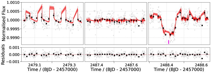
Figure 8: Results of the global photometric fit. This plot shows the six CHEOPS lightcurves, where the 60 second cadence data (grey) has been binned to 20 minutes (black squares) to guide the eye. The red line is the median model from the global photometric fit and the red shaded region is the 1$\sigma$ uncertainty on the model. The blue and pink markers indicate the mid-transit times of the inner and outer planets, respectively. The residuals of the model are included in the panel beneath each lightcurve.

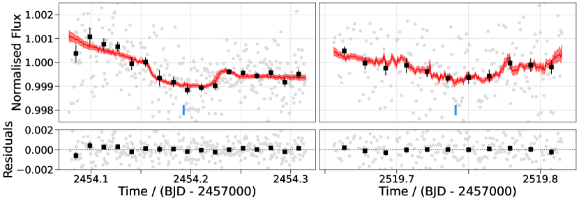
Figure 9: Results of the global photometric fit. This plot shows the two LCOGT lightcurves, where the 60 second cadence data (grey) has been binned to 20 minutes (black squares) to guide the eye. The red line is the median model from the global photometric fit and the red shaded region is the 1$\sigma$ uncertainty on the model. The blue markers indicate the mid-transit times of the inner planet. The residuals of the model are included in the panel beneath each lightcurve.

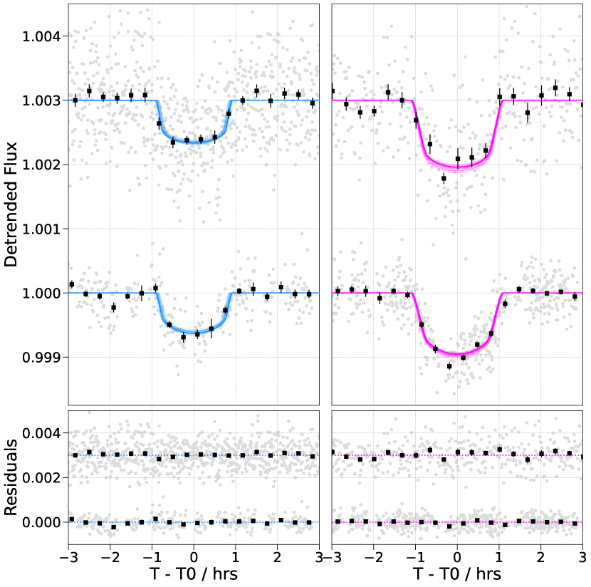
Figure 10: Results of the global photometric fit. Upper: Phase-folded TESS (top) and CHEOPS (bottom) lightcurves for the inner (left) and outer (right) planet. The lightcurves have been detrended to remove the instrumental and stellar variability and the data (grey) has been binned to 20 minutes (black squares) to guide the eye. The median transit models for the inner (blue line) and outer (pink line) planet are included, along with 50 random samples drawn from the posterior distribution of the model. Lower: Residuals of the median transit models. Note that an arbitrary offset has been applied to the TESS data and residuals for visibility purposes.

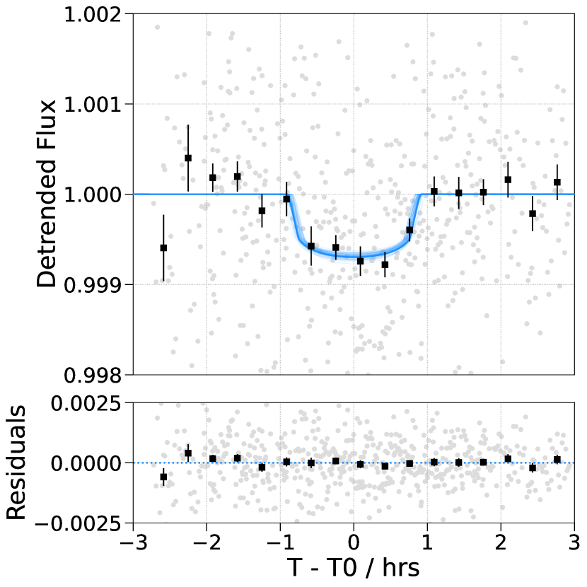
Figure 11: Results of the global photometric fit. Upper: Phase-folded LCOGT lightcurve for the inner planet. The lightcurve has been detrended to remove instrumental effects and the data (grey) has been binned to 20 minutes (black squares) to guide the eye. The median transit model for the inner planet (blue line) is included, along with 50 random samples drawn from the posterior distribution of the model. Lower: Residuals of the median transit model.

Our analysis has shown that HD 15906 b is a 2.24 R_⊕ planet orbiting its host star at a separation of 0.090 AU with a period of 10.92 days. HD 15906 c is bigger (2.93 R_⊕) and orbits the host star at a larger separation (0.141 AU) with a longer period (21.58 days). The fit favoured slightly eccentric orbits (e${}_{\text{b}}$ = 0.11, e${}_{\text{c}}$ = 0.04) with a high impact parameter (b${}_{\text{b}}$ = 0.86, b${}_{\text{c}}$ = 0.90), but the transits of both planets are non-grazing. The inner and outer planet receive 33.1 and 13.4 times the amount of flux that the Earth receives from the Sun and, assuming zero bond albedo and full day-night heat redistribution, they have equilibrium temperatures of 668 and 532 K. We remind the reader that we repeated our global photometric fit with zero eccentricity and all fitted planet parameters were consistent within 1.2$\sigma$. In this case, we derived planetary radii of 2.24 $\pm$ 0.07 R_⊕ and 2.84 $\pm$ 0.05 R_⊕ for HD 15906 b and c, respectively.

5.2 Transit Timing Variation Results

In Section 4.3, we described our TTV analysis of the HD 15906 system. The fitted observed transit times for each planet are presented in Table 8. From these values, juliet derived the best-fitting period and mid-transit time for each planet, assuming a linear ephemeris. These values, and all other fitted planet parameters, were fully consistent with the results of the global photometric model (see Section 5.1) within 2$\sigma$.

Table 8: Observed mid-transit times for HD 15906 b and c from the TTV analysis presented in Section 4.3

Mid-transit time / (BJD - 2457000)	Instrument
HD 15906 b
1416.3499${}^{+0.0033}_{-0.0039}$	TESS
1427.2780${}^{+0.0037}_{-0.0053}$	TESS
2148.2970${}^{+0.0017}_{-0.0016}$	TESS
2159.2181${}^{+0.0050}_{-0.0048}$	TESS
2454.1965${}^{+0.0027}_{-0.0034}$	LCOGT
2497.8933 $\pm$ 0.0009	CHEOPS
2519.7323${}^{+0.0056}_{-0.0050}$	LCOGT
HD 15906 c
1430.8323${}^{+0.0031}_{-0.0033}$	TESS
2164.6570 $\pm$ 0.0022	TESS
2488.4142 $\pm$ 0.0007	CHEOPS
2531.5753 $\pm$ 0.0008	CHEOPS

Using the best-fitting period and mid-transit time, we computed the expected transit times for each planet. We then plotted an observed - computed (O-C) diagram, see Figure 12, to show the TTVs. We found marginal evidence for TTVs – the maximum TTV is $\sim$ 10 minutes, but nine of the eleven transits are consistent with no TTVs within 3$\sigma$. With only eleven transits of two planets and a gap of $\sim$ 2 years in the data, we did not attempt to model these TTVs. In Section 7.2, we simulate the expected TTV signals for the two planets and compare these predictions with the observations.

Figure 12: Results of the TTV analysis. This plot shows the difference between the observed (O) transit time and the computed (C) transit time, assuming a linear ephemeris, for transits of the inner (blue) and outer (pink) planet from TESS (square), CHEOPS (diamond) and LCOGT (circle).

5.3 Radial Velocity Results

In an attempt to detect the two planetary signals in the HARPS and FIES data, we fit five models to the RVs (see Section 4.4). We tried a model with no planets, only the inner and outer planet, both planets and both planets plus a GP to model the stellar activity. In the fit with the GP, the posterior distributions of the GP hyperparameters were the same as the priors, which tells us the data was unable to constrain the GP model, as expected. In Table 9, we present the Bayes evidence of each fit compared to the fit with no planets. The model with no planets had the highest evidence, with a substantial or strong preference over the other models (Kass & Raftery, 1995), and we therefore conclude that the two transiting planets are not detected in the current HARPS and FIES RV data. However, we can still utilise this data for validation purposes, see Section 6.1.

Table 9: Comparison of the Bayes evidence from our HARPS and FIES RV fits. The difference in Bayes evidence (dlnZ) between each fit and the fit with no planets is quoted. The model with no planets was preferred over the more complex models.

Model	dlnZ
No Planets	0.0
Inner Planet Only	-2.1
Outer Planet Only	-1.6
Two Planets	-3.9
Two Planets and GP	-3.7

6 Vetting and Validation

It is important to confirm that the transits we observed with TESS, CHEOPS and LCOGT were caused by planets orbiting HD 15906. We therefore need to rule out false positive scenarios, including:

1. The target star is an eclipsing binary (EB).

2. The target star has a gravitationally associated companion star that is either an EB or has transiting planets.

3. There is an aligned foreground or background star, not gravitationally associated with the target star, that is either an EB or has transiting planets.

4. There is a nearby star, with a small angular separation from the target star but not gravitationally associated with it, that is either an EB or has transiting planets.

Furthermore, it is important to check for nearby unresolved stars because, if not accounted for, the blended flux can lead to underestimated planetary radii and improper characterisation of the host star (Ciardi et al., 2015; Furlan & Howell, 2017, 2020).

As mentioned in Section 2.1, HD 15906 b passed all of the SPOC vetting tests. In addition, it has been shown that multiplanet systems are significantly less likely to be false positives than single planet systems, especially when the planets are smaller than 6 R_⊕ (Lissauer et al., 2012; Guerrero et al., 2021). In this section, we use additional observational and statistical techniques to validate the HD 15906 planetary system.

6.1 High-Resolution Spectroscopy

Using the HARPS and FIES data, we did not detect the RV signals induced by the two transiting objects (see Section 5.3). In this section, we use the HARPS data to rule out stellar masses for the transiting objects and place limits on the presence of a bound stellar companion.

In Figure 13, we show the HARPS and FIES RVs folded on HD 15906 b and c using the ephemerides obtained in the global photometric analysis (Table 7).

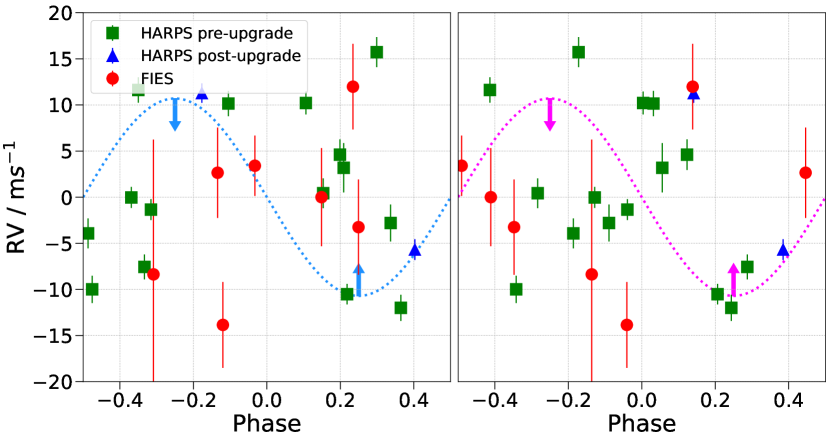
Figure 13: HARPS (green squares and blue triangles) and FIES (red circles) RV data folded on the inner (left) and outer (right) planet. The transits occur at phase zero. A Keplerian model (dotted line) has been plotted on each axis to guide the eye and the arrows illustrate that this is an upper limit. The model represents a planet on a circular orbit with a semi-amplitude equivalent to the RMS of the HARPS data (10.70 ms^-1), a proxy for its maximum value.

The RMS of the HARPS data (10.70 ms^-1) can be used as a proxy for the maximum possible semi-amplitudes of the two transiting objects. Using the stellar mass presented in Table 5, the orbital parameters presented in Table 7 and a semi-amplitude of 10.70 ms^-1, HD 15906 b has an upper mass limit of $\sim$ 32 M_⊕ and HD 15906 c has an upper mass limit of $\sim$ 39 M_⊕. This confirms that the two transiting objects must be of planetary mass.

Furthermore, under the assumption of a circular orbit and an orbital inclination of 90 degrees, the RMS of the HARPS data rules out a bound brown dwarf or star, with a mass greater than 13 M${}_{\text{Jupiter}}$, out to $\sim$ 1500 AU. At the distance of HD 15906, this corresponds to an angular separation of $\sim$ 32″. Even down to an orbital inclination of 10 degrees, we can rule out a brown dwarf or stellar companion out to $\sim$ 45 AU, corresponding to an angular separation of $\sim$ 1″.

Finally, we checked for a linear drift in the RV data because this could be indicative of a long-period bound stellar companion. We chose the pre-upgrade HARPS data for this purpose because it has the longest baseline ($>$ 9 years). We used juliet to perform a fit of this data, using a model consisting of no planets, an offset, white noise and a linear trend. The best-fit gradient was consistent with zero within 1$\sigma$ and this supports the conclusion that HD 15906 does not have a bound stellar companion.

6.2 Archival Imaging

HD 15906 is a high proper motion star ($\mu$ = 195.97 mas yr^-1; Gaia Collaboration et al., 2022). We therefore made use of archival imaging to check for foreground or background objects at the star’s present day position.

HD 15906 was observed on 11 November 1953 by the Oschin Schmidt Telescope, using a blue photographic emulsion ($\lambda$ = 330 - 500 nm; Monet et al., 2003), during the first Palomar Observatory Sky Survey (POSS-I). It was observed again on 21 September 1979 by the UK Schmidt Telescope, using a blue photographic emulsion ($\lambda$ = 395 - 540 nm; Monet et al., 2003), during the SERC-EJ survey. We downloaded these images from the Digitized Sky Survey (DSS) and plotted them in the first two panels of Figure 14. HD 15906 was also observed in 2010 by the Panoramic Survey Telescope and Rapid Response System (Pan-STARRS; Chambers et al., 2016). We downloaded the i-filter Pan-STARRS image from the MAST and plotted it in the third panel of Figure 14. Finally, HD 15906 was observed during TESS sector 31 in 2020. We downloaded the target pixel file (TPF) from the MAST and plotted the first good quality cadence in the final panel of Figure 14.

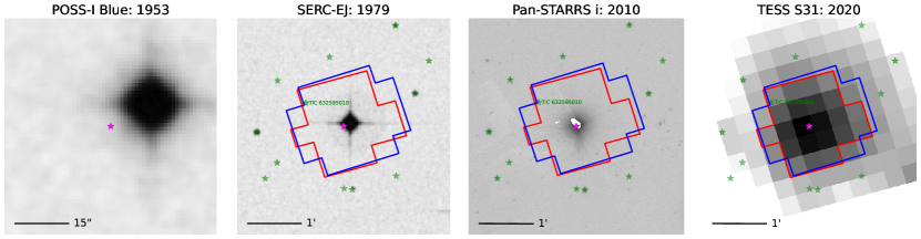
Figure 14: Images of HD 15906 spanning 67 years, from 1953 to 2020. Left to right: POSS-I, SERC-EJ, Pan-STARRS and TESS sector 31. All images are shown on a scale of 4′ $\times$ 4′, except for the POSS-I image which is zoomed in to 1′ $\times$ 1′, and centred on the 2020 position of HD 15906 (pink star). We overlaid the TESS apertures from sector 4 (blue) and sector 31 (red) on the images, as well as the 2020 positions of all known stars from Gaia DR3 (green stars; Gaia Collaboration et al., 2022). Only one of these stars (TIC 632595010; TESS magnitude = 20.3) is within the TESS apertures.

HD 15906 moved $\sim$ 13″ between the POSS-I observation in 1953 and TESS sector 31 in 2020. Using the POSS-I image, we rule out a foreground or background star at the TESS sector 31 position of HD 15906 down to a TESS magnitude of $\sim$ 18. A star this faint would be incapable of producing the transit signals we observe, even in the case of a full EB, and it would not significantly impact the derived planet parameters due to flux blending (Ciardi et al., 2015). We therefore conclude that our results are not affected by an unresolved foreground or background star.

6.3 High-Resolution Imaging

High-resolution imaging was used to search for nearby stars, bound or unbound, that could be contaminating the photometry. We observed HD 15906 with a combination of high-resolution resources, including near-infrared adaptive optics (NIR AO) imaging at the Keck and Lick Observatories and optical speckle imaging at Gemini-North and SOAR. While the optical observations tend to provide higher resolution, the NIR AO tend to provide better sensitivity, especially to lower-mass stars. The combination of the observations in multiple filters enables better characterisation of any companions that might be detected. The observations are described in detail in the following subsections and a summary is provided in Table 10. Figure 15 shows the resulting images and contrast curves. No stellar companions were detected within the contrast and angular limits of each facility, essentially ruling out stars at least $\sim$ 7 magnitudes fainter than HD 15906 between 0.5″ and 10″. At small angular separations, where high-resolution imaging does not achieve a high contrast, we used high-resolution spectroscopy to rule out bound companions within $\sim$ 1″ (see Section 6.1).

Table 10: A summary of the high-resolution imaging observations of HD 15906.

Facility	Instrument	Filter	Date [UTC]
SOAR	HRCam	Cousins-I	2019-07-14
Lick	ShARCS	$Ks$	2019-07-21
Gemini-North	’Alopeke	562 nm	2019-10-15
Gemini-North	’Alopeke	832 nm	2019-10-15
Keck	NIRC2	Br-$\gamma$	2020-09-09

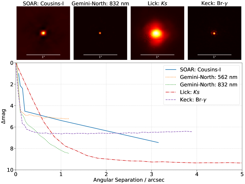
Figure 15: High-resolution imaging of HD 15906. Upper: From left to right are the speckle images from SOAR and Gemini-North and the NIR AO images from Lick and Keck. Each image is zoomed into a region of 1.6″ $\times$ 1.6″centred on HD 15906. Lower: Contrast curves from each observation.

6.3.1 SOAR

We searched for stellar companions to HD 15906 with speckle imaging on the 4.1 m Southern Astrophysical Research (SOAR) telescope (Tokovinin, 2018) on 14 July 2019. We observed in Cousins I-band, a similar visible bandpass to TESS. This observation was sensitive to a star 5.3 magnitudes fainter than HD 15906 at an angular distance of 1″ from the target. More details of the observations within the SOAR TESS survey are available in Ziegler et al. (2020). The 5$\sigma$ detection sensitivity and speckle auto-correlation functions from the observations are shown in Figure 15. No nearby stars were detected within 3″ ($\sim$ 137 AU, if bound) of HD 15906 in the SOAR observations.

6.3.2 Lick

We observed HD 15906 on 21 July 2019 using the Shane Adaptive optics infraRed Camera-Spectrograph (ShARCS) camera on the Shane 3 m telescope at Lick Observatory (Kupke et al., 2012; Gavel et al., 2014; McGurk et al., 2014). Observations were taken with the Shane AO system in natural guide star mode in order to search for nearby, unresolved stellar companions. We collected a single sequence of observations using a $Ks$ filter ($\lambda_{0}$ = 2.150 $\mu$m, $\Delta\lambda$ = 0.320 $\mu$m). We reduced the data using the publicly available SImMER pipeline(Savel et al., 2020). Our reduced image and corresponding contrast curve is shown in Figure 15. The observations rule out stellar companions $\sim$ 4 magnitudes fainter than HD 15906 at 0.5″ ($\sim$ 23 AU, if bound) and $\sim$ 9 magnitudes fainter between 2″ and 10″ ($\sim$ 92 - 458 AU, if bound).

6.3.3 Gemini-North

HD 15906 was observed on 15 October 2019 using the ’Alopeke speckle instrument on the Gemini-North 8 m telescope (Scott et al., 2021; Howell & Furlan, 2022). ’Alopeke provides simultaneous speckle imaging in two bands (562 nm and 832 nm) with output data products including a reconstructed image with robust contrast limits on companion detections. Three sets of 1000 $\times$ 0.06 second images were obtained and processed in our standard reduction pipeline (see Howell et al., 2011). Figure 15 includes our final 5$\sigma$ contrast curves and the 832 nm reconstructed speckle image. We find that HD 15906 has no companion stars brighter than 5-8 magnitudes below that of the target star within the angular and image contrast levels achieved. The angular region covered ranges from the 8 m telescope diffraction limit (20 mas) out to 1.2″ ($\sim$ 0.9 to 55 AU, if bound).

6.3.4 Keck

HD 15906 was observed with NIR AO high-resolution imaging at the Keck Observatory on 9 September 2020. The observations were made with the NIRC2 instrument, which was positioned behind the natural guide star AO system (Wizinowich et al., 2000), on the Keck-II telescope. We used the standard 3-point dither pattern to avoid the lower left quadrant of the detector which is typically noisier than the other three quadrants. The dither pattern step size was 3″ and was repeated twice, with each dither offset from the previous dither by 0.5″. The camera was in the narrow-angle mode with a full field of view of $\sim$ 10″ and a pixel scale of approximately 0.0099442″pix^-1. The observations were made in the narrow-band Br-$\gamma$ filter ($\lambda_{0}$ = 2.1686 $\mu$m, $\Delta\lambda$ = 0.0326 $\mu$m) with an integration time of 0.5 second with one co-add per frame for a total of 4.5 seconds on target. The AO data were processed and analysed with a custom set of IDL tools (see description in Schlieder et al., 2021) and the resolution of the final combined image, determined from the FWHM of the PSF, was 0.048″. The sensitivity of the combined AO image was determined according to Furlan et al. (2017) and the resulting sensitivity curve for the Keck data is shown in Figure 15. The image reaches a contrast of $\sim$ 7 magnitudes fainter than the host star between 0.5″ and 4″ ($\sim$ 23 to 183 AU, if bound) and no stellar companions were detected.

6.4 Gaia Assessment

We used Gaia DR3 (Gaia Collaboration et al., 2022) to show that there are no nearby, resolved stars bright enough to cause the transits we observe. The images presented in Figure 14 show that there is only one Gaia DR3 star within the TESS optimal apertures. This is TIC 632595010 with a TESS magnitude of 20.3 ($>$ 10 mag fainter than HD 15906) and a separation of $\sim$ 50″ from HD 15906. This star is not bright enough to be the source of the transit signals we see, even in the case of a full EB. Furthermore, as explained in Section 2.3, the LCOGT observations confirmed that the transit signals do not originate from any of the known Gaia DR3 stars.

We also searched for wide stellar companions that may be bound members of the system. Based upon similar parallaxes and proper motions (Mugrauer & Michel, 2020, 2021), there are no additional widely separated companions identified by Gaia.

Finally, the Gaia DR3 astrometry provides additional information on the possibility of inner companions that may have gone undetected by either Gaia or the high-resolution imaging/spectroscopy. The Gaia Renormalised Unit Weight Error (RUWE) is a metric, similar to a reduced chi-square, where values that are $\lesssim$ 1.4 indicate that the Gaia astrometric solution is consistent with a single star whereas RUWE values $\gtrsim$ 1.4 may indicate an astrometric excess noise, possibly caused by the presence of an unseen companion (e.g., Ziegler et al., 2020). HD 15906 has a Gaia DR3 RUWE value of 1.15, indicating that the astrometric fits are consistent with a single star model.

6.5 Statistical Validation

We finally used TRICERATOPS (Tool for Rating Interesting Candidate Exoplanets and Reliability Analysis of Transits Originating from Proximate Stars; Giacalone et al., 2021) to statistically validate the two transiting planets in the HD 15906 system. This Bayesian tool uses the stellar and planet parameters, the transit lightcurve and the high-resolution imaging to test the false positive scenarios listed at the start of Section 6 and calculate the false positive probability (FPP) and the nearby false positive probability (NFPP) of TESS planet candidates. The FPP is the probability that the observed transit is not caused by a planet on the target star and the NFPP is the probability that the observed transit originates from a resolved nearby star. To consider a planet candidate validated, it must have FPP $<$ 0.015 and NFPP $<$ 0.001.

We ran TRICERATOPS on both HD 15906 b and c. We used the stellar parameters presented in Table 5, the planet parameters presented in Table 7, the combined TESS, CHEOPS and LCOGT lightcurve and the high-resolution imaging contrast curves from Section 6.3. TRICERATOPS only accepts one contrast curve as input, so we ran the analysis with each of the five contrast curves and compared the results. In agreement with our analysis in Section 6.4, TRICERATOPS did not identify any nearby resolved stars that were bright enough to be the source of the transits. The results confirmed that the highest probability scenario was that of two planets transiting HD 15906. The most probable form of false positive scenario for the inner planet was an unresolved background EB and for the outer planet was an unresolved bound companion that is an EB. With our archival imaging (Section 6.2) and high-resolution spectroscopy (Section 6.1), that TRICERATOPS does not consider, these scenarios become less likely. For the Gemini-North and Keck contrast curves, both planets were validated with a negligible value of NFPP and FPP $<$ 0.015. With the SOAR and Lick contrast curves, both planets had a negligible value of NFPP, the outer planet had FPP $<$ 0.015 and the inner planet had a FPP just greater than 0.015 (0.0159 for Lick and 0.0166 for SOAR). According to the TRICERATOPS criteria, this means that the inner signal is likely a planet. However, TRICERATOPS does not account for the fact that multiplanet systems are more likely to be real (Lissauer et al., 2012; Guerrero et al., 2021), so the fact that the outer planet was validated means the inner planet may also be considered validated. We therefore conclude that both HD 15906 b and c are validated planets according to the TRICERATOPS criteria.

7 Discussion

We have presented the discovery of the HD 15906 multiplanet system. In this section, we discuss our results, compare the system to other confirmed exoplanets and assess the feasibility of future follow-up observations.

7.1 TESS Periodicity

In Section 4.2.3, we reported the detection of a sinusoidal-like signal in the TESS sector 4 lightcurve of HD 15906. This signal has a period of 0.22004 days ($\sim$ 5 hours) and the best-fit sinusoidal model has an amplitude of $\sim$ 57 ppm, equivalent to the transit depth expected for a planet with a radius of $\sim$ 0.63 R_⊕. In this section, we provide a discussion of this signal and its origin.

The 0.22 day periodic signal is present in the TESS sector 4 lightcurve, but not the sector 31 lightcurve. The signal is present in the sector 4 SAP and PDCSAP flux, but not in the background flux or centroid position. We checked for a periodic signal in the nearest star of comparable magnitude (TIC 4646803; TESS magnitude = 9.51, separation = 167″). This star was observed at 30 minute cadence in sector 4, so we searched the TESS-SPOC lightcurve (Caldwell et al., 2020) and found no periodicity at 0.22 days.

We also extracted our own HD 15906 lightcurves from the TESS TPFs for both sectors. This was done using a default quality bitmask and optimising the aperture mask to reduce the combined differential photometric precision (CDPP) noise in the resulting data. The extracted target fluxes were sky-corrected using a custom background mask. Detrending was done in two steps: scattered light was corrected for using a principal component analysis and any flux modulation caused by spacecraft jitter was removed by a linear model detrending using co-trending basis vectors and the mean and average of the engineering quaternions as the basis vectors. This second method has shown promise in cleaning up TESS photometry previously (Delrez et al., 2021). Our lightcurves were consistent with the TESS SAP and PDCSAP flux; our sector 4 lightcurve contained a 0.22 day periodicity and our sector 31 lightcurve did not. We can therefore confirm that the periodic signal is not dependent on lightcurve extraction technique.

Furthermore, we performed experiments extracting lightcurves from apertures of different sizes and found that using an aperture of radius 1 pixel centred on HD 15906 resulted in a significantly larger amplitude variability (roughly by a factor of two) than when we used an aperture of radius 4 pixels. This is not what we would expect for a signal originating from within a pixel of HD 15906 (where we would expect the amplitude to stay roughly constant given the lack of nearby bright stars to dilute the flux) or from a blended star from larger distances (which should show larger amplitude in larger apertures).

We considered the possibility that the periodic signal is a form of stellar activity originating from HD 15906. However, a variety of arguments suggested that this was unlikely. Firstly, the signal is strongly present in TESS sector 4, but is undetectable in any other observations. The very short period of the signal strongly disfavours it being related to the rotation period of HD 15906, given the star’s narrow spectral lines and amenability to precise RV measurements. The period ($\sim$ 5 hours) is consistent with the timescale of granulation on the surface of a Sun-like star, but this process does not create sharp periodicities like we detected (see Figure 6, which shows a clearly defined sharp peak in the periodogram of the sector 4 TESS residuals). Stellar pulsations can sometimes create such sharp periodicities, but main sequence stars of this type should not exhibit any pulsations on similar amplitudes or timescales.

We finally searched for evidence that the signal originated from another star on the TESS detectors and contaminated the lightcurve of HD 15906 through a process other than direct overlap of the PSFs. This was a frequent occurrence during the Kepler and K2 missions (Coughlin et al., 2014) but is much less common during the TESS mission due to differences in the design of the telescopes, electronics and optics. The bright contact binary DY Cet (TIC 441128066; TESS magnitude = 9.23) was observed on the same CCD as HD 15906 during TESS sectors 4 and 31. This EB has a period of 0.4408 days and the TESS lightcurves show a sinusoidal-like variability with a period of 0.2204 days (Yıldırım, 2022). This is consistent with the period of the signal we detected in the TESS sector 4 lightcurve of HD 15906. During sector 4, DY Cet was in the same CCD columns as HD 15906, but during sector 31 it was not. We therefore conclude that the flux from DY Cet contaminated that of HD 15906 in TESS sector 4 during CCD readout, although the exact mechanism of contamination is currently unknown. We note that DY Cet cannot be the source of the transits of HD 15906 b and c, which have been independently observed by CHEOPS and LCOGT, and we reiterate that this periodic signal does not affect our fitted planet parameters (see Section 4.2.3).

7.2 Transit Timing Variation Predictions

In Section 5.2, we reported marginal evidence for TTVs in the HD 15906 system. Here, we compute the expected TTV signals for each planet and compare them with our observations. We reiterate that modelling the TTVs is beyond the scope of this work due to the small amount of data.

We compared two methods for simulating the TTV signals of HD 15906 b and c. The first uses an approximated estimation of the TTV signal by modelling it as a linear combination of basis functions as described in Hadden et al. (2019) and implemented in the TTV2Fast2Furious package. The second approach is a direct N-body simulation with the TRADES code (Borsato et al., 2014; Borsato et al., 2019; Nascimbeni et al., 2023). For each planet, we used the orbital period and inclination presented in Table 7, the predicted mass (see Section 7.4.1) and we assumed a circular orbit for simplicity. We simulated the TTV signal for planets b and c for a time range that covers the full range of transit observations and we present the results in Figure 16.

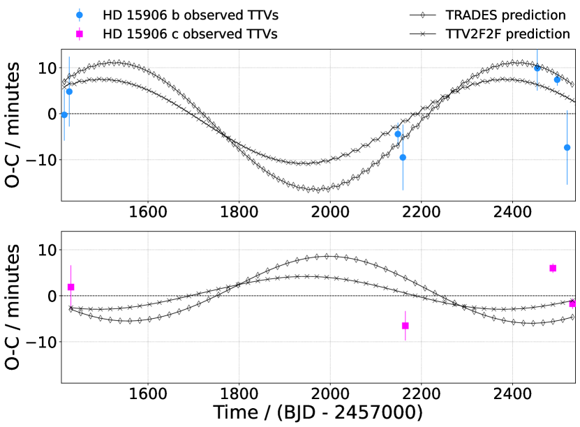
Figure 16: The predicted TTV signal, as computed with TTV2Fast2Furious (TTV2F2F, crosses and solid line) and TRADES (open diamonds and solid line), for HD 15906 b (upper panel) and HD 15906 c (lower panel). We have also included the observed TTVs for each planet (blue circles and pink squares).

The predictions for HD 15906 b are generally in good agreement with the observations. We note that there is a slight difference between the amplitudes of the two simulated TTV signals, but both are consistent with most of the observations given their uncertainties. However, the predictions for HD 15906 c seem to be in anti-phase with the observations. As expected for a two planet configuration close to a first-order period commensurability, the predicted TTVs of planets b and c are anti-correlated (Agol & Fabrycky, 2018). Contrary to this expectation, the observed TTVs of HD 15906 b and c appear to be correlated. This could suggest that there is an additional, undetected planet in the system perturbing the orbits of the two observed planets. Alternatively, the TTVs might be spurious or affected by excess systematic noise from, for example, stellar activity (e.g., Oshagh et al., 2013; Ioannidis et al., 2016). Given the sparse sampling of the TTV signals, future observations are required to assess the true nature of the TTVs.

7.3 Comparison with Confirmed Exoplanets

HD 15906 b and c have radii of 2.24 R_⊕ and 2.93 R_⊕, respectively, meaning they cannot have a purely rocky composition (Rogers, 2015; Lozovsky et al., 2018). They both fall on the upper side of the radius gap and we therefore classify them as sub-Neptunes. Furthermore, with insolation fluxes of 33 S_⊕ and 13 S_⊕, and equilibrium temperatures of 668 K and 532 K, both planets are in the warm regime (T${}_{\text{eq}}\lesssim$ 700 K).

Of more than 5300 confirmed exoplanets, there are 66 sub-Neptune sized planets (1.75 $<$ R${}_{\text{P}}$ / R_⊕ $<$ 3.5) transiting bright stars (G $\leq$ 10 mag). Only 18 of these have an insolation flux less than HD 15906 b and only 5 have an insolation flux lower than HD 15906 c – GJ 143 b (Dragomir et al., 2019), $\nu^{2}$ Lupi d (Delrez et al., 2021), HD 23472 c (Barros et al., 2022), HD 73583 c (Barragán et al., 2022) and Kepler-37 d (Marcy et al., 2014). HD 15906 c is therefore one of the most lowly irradiated sub-Neptune planets transiting such a bright star. Furthermore, there are only 5 other multiplanet systems with two warm (T${}_{\text{eq}}\leq$ 700 K) sub-Neptune sized planets (1.75 $<$ R${}_{\text{P}}$ / R_⊕ $<$ 3.5) transiting a bright (G $\leq$ 10 mag) star – HD 108236 (Bonfanti et al., 2021), $\nu^{2}$ Lupi (Delrez et al., 2021), HD 191939 (Orell-Miquel et al., 2023), HD 23472 (Barros et al., 2022) and TOI 2076 (Osborn et al., 2022). The HD 15906 system is therefore an interesting target for future follow-up studies, discussed further in Section 7.4.

Due to the nature of its observing strategy, TESS is biased towards the discovery of short-period planets; less than 14% of planets confirmed by TESS have periods longer than 20 days, of which only half have radii smaller than 4 R_⊕. This work has demonstrated how CHEOPS can be used to follow-up TESS duotransits to expand the sample of long-period planets. Figure 17 presents a period-radius diagram comparing the two planets in the HD 15906 system to the confirmed exoplanet population. The other TESS duotransits resolved by CHEOPS have also been included – TOI 2076 c and d (Osborn et al., 2022), HIP 9618 c (Osborn et al., 2023), TOI 5678 b (Ulmer-Moll et al., 2023) and HD 22946 d (Garai et al., 2023). Through our CHEOPS duotransit programme, we have contributed to the discovery of 6 planets with periods longer than 20 days, radii smaller than 5 R_⊕ and host stars brighter than G = 12 mag. There are only 18 other planets confirmed by TESS in this parameter space, illustrating the power of the TESS and CHEOPS synergy for the discovery of small, long-period planets transiting bright stars.

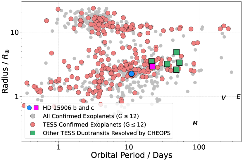
Figure 17: Period-radius diagram of confirmed exoplanets with a Gaia magnitude brighter than 12, where discoveries made by TESS are highlighted in red. HD 15906 b (blue circle) and c (pink square) are included, alongside the five additional TESS duotransits resolved by CHEOPS (green squares).

7.4 Potential for Future Follow-Up

With two warm sub-Neptunes transiting a bright (G $\sim$ 9.5 mag) K-dwarf, the HD 15906 system is an excellent target for future observations to measure the masses of the planets and perform atmospheric characterisation. Warm sub-Neptunes are less affected by radiation from their host star than their hot counterparts, meaning their atmospheres will not have been sculpted so heavily by photoevaporation and they will more closely resemble their primordial state. Observations of these planets are therefore crucial in testing models of the formation and evolution of sub-Neptune planets. In addition, as a multiplanet system, HD 15906 will allow for comparative studies of internal structure and composition as a function of stellar irradiation.

7.4.1 Radial Velocity

We were unable to detect HD 15906 b and c in the current HARPS and FIES RV data due to the small number of sparsely sampled observations (see Figure 7 and Section 5.3). Here, we use the results of our global photometric analysis (Table 7) to predict the expected mass and semi-amplitude of the two planets. Otegi et al. (2020) present a mass-radius relation that is dependent upon the density of the planet ($\rho_{\text{P}}$):

$$\text{M}_{\text{P}}=\begin{cases}(0.90\pm 0.06){\text{R}_{\text{P}}}^{3.45\pm 0.12},&\text{if }\rho_{\text{P}}>3.3gcm^{-3}\\ (1.74\pm 0.38){\text{R}_{\text{P}}}^{1.58\pm 0.10},&\text{if }\rho_{\text{P}}<3.3gcm^{-3}\end{cases}$$ (1)

The high density case is applicable when the planet has a rocky composition and the low density case is for when the planet has a volatile-rich composition. Assuming a volatile-rich composition, the inner and outer planet would have masses of 6.21${}^{+1.56}_{-1.43}$M_⊕ and 9.47${}^{+2.44}_{-2.21}$M_⊕, respectively, leading to semi-amplitudes of 2.11${}^{+0.53}_{-0.49}$ms^-1 and 2.54${}^{+0.67}_{-0.60}$ms^-1.

The predicted semi-amplitudes of HD 15906 b and c are greater than the average HARPS RV uncertainty ($\sim$ 1.5 ms^-1). This means that the planetary signals should be detectable with sufficient observations from a high-resolution spectrograph. Since HD 15906 is visible from both hemispheres, there are many instruments that would be capable of doing this. We note that there is a relatively large scatter in the current RV data ($\sim$ 10 ms^-1) which could make a precise mass measurement challenging. It will require a high sampling rate and a large number of RV observations to adequately model the planetary and stellar signals.

7.4.2 Atmospheric Characterisation

Theory predicts a wide variety of possible chemical compositions for sub-Neptunes (e.g., Moses et al., 2013; Guzmán-Mesa et al., 2022). Atmospheric characterisation can constrain their composition and, thanks to their bright host star, HD 15906 b and c are amenable to such observations. The Transmission Spectroscopy Metric (TSM; Kempton et al., 2018) can be used to rank transiting planets based on their suitability for transmission spectroscopy. It quantifies the expected SNR of the spectral features for a 10 hour observation with JWST/NIRISS, assuming a cloud-free atmosphere. Using the stellar parameters from Table 5 and planet parameters from Table 7, we find that HD 15906 b and c have TSM values of 71.7 and 82.1, respectively. This puts them in the top 3% of all confirmed transiting planets smaller than 4 R_⊕, where in the absence of a measured mass we computed the expected mass according to the empirical mass-radius relation used by Kempton et al. (2018). Furthermore, HD 15906 b and c have amongst the highest TSMs for such small and lowly irradiated planets, illustrated in Figure 18. There are only 6 sub-Neptune sized planets (1.75 $<$ R${}_{\text{P}}$ / R_⊕ $<$ 3.5) with a higher TSM and lower irradiation than HD 15906 c, of which HD 15906 is the second brightest host star. In addition, there are only 3 other multiplanet systems which host 2 sub-Neptune sized planets with irradiation lower than 35 S_⊕ and TSM higher than 70 (HD 191939, TOI 2076 and TOI 270; Orell-Miquel et al., 2023; Osborn et al., 2022; Van Eylen et al., 2021). The HD 15906 system is therefore an interesting target for comparative studies of warm sub-Neptune composition.

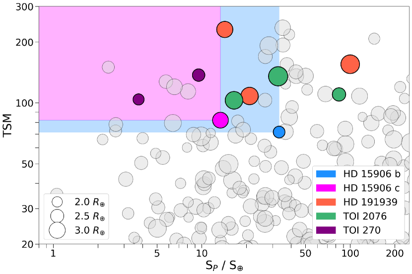
Figure 18: Transmission spectroscopy metric (TSM) as a function of stellar irradiation for all confirmed sub-Neptune sized planets (1.75 $<$ R${}_{\text{P}}$ / R_⊕ $<$ 3.5). The marker size scales with planet radius and HD 15906 b (blue) and c (pink) are plotted alongside a shaded region to show planets with a lower irradiation and higher TSM. HD 15906 is one of 4 multiplanet systems with 2 sub-Neptune sized planets with irradiation lower than 35 S_⊕ and TSM higher than 70. The other 3 systems are highlighted in red (HD 191939), green (TOI 2076) and purple (TOI 270).

8 Conclusions

In this paper, we have reported the discovery and validation of two warm sub-Neptune planets transiting the bright (G = 9.5 mag) K-dwarf HD 15906 (TOI 461, TIC 4646810). During TESS sectors 4 and 31, four transits of the inner planet, HD 15906 b, were observed, but there were only two transits of the outer planet, HD 15906 c, separated by $\sim$ 734 days. The period of the outer planet was ambiguous, with 36 possible values, and we used CHEOPS follow-up to determine the true period. Using TESS, CHEOPS and LCOGT photometry, we precisely characterised the two planets – HD 15906 b and c have periods of 10.92 days and 21.58 days and radii of 2.24 R_⊕ and 2.93 R_⊕, respectively. We found marginal evidence for TTVs in the system and, comparing the observations to simulations, we showed that more observations are required to understand the nature of the TTV signals. Both planets are in the warm regime, with insolation fluxes of 33.1 S_⊕ and 13.4 S_⊕ and equilibrium temperatures of 668 K and 532 K. We find that HD 15906 c is one of the most lowly irradiated sub-Neptune sized planets transiting such a bright star.

Both HD 15906 b and c are prime targets for future detailed characterisation studies. They are amenable to precise mass measurement and they are amongst the top warm sub-Neptune candidates for atmospheric characterisation with JWST. These studies will allow us to constrain the compositions of HD 15906 b and c, test planet formation and evolution models and improve our limited understanding of sub-Neptune planets as a whole.

Data Availability

The TESS data used in this paper is publicly available on the MAST (https://mast.stsci.edu/portal/Mashup/Clients/Mast/Portal.html). The CHEOPS DRP data products are publicly available on the CHEOPS mission archive (https://cheops.unige.ch/archive_browser/). The raw and detrended CHEOPS PIPE lightcurves and the WASP photometry have been made available online at the CDS (https://cdsarc.cds.unistra.fr/viz-bin/cat/J/MNRAS/523/3090). The LCOGT data and high-resolution imaging are publicly available on ExoFOP (https://exofop.ipac.caltech.edu/tess/). The HARPS spectra are publicly available on the ESO Science Archive (http://archive.eso.org/cms.html) and the HARPS RVs were taken from Trifonov et al. (2020). The HARPS and FIES RVs used in our analysis are presented in Table 4. The archival imaging is publicly available at the Digitized Sky Survey (https://archive.stsci.edu/cgi-bin/dss_form) and the MAST.

Affiliations

¹Astrophysics Group, Cavendish Laboratory, University of Cambridge, JJ Thomson Avenue, Cambridge CB3 0HE, UK
²ETH Zurich, Department of Physics, Wolfgang-Pauli-Strasse 2, CH-8093 Zurich, Switzerland
³Center for Space and Habitability, University of Bern, Gesellschaftsstrasse 6, 3012 Bern, Switzerland
⁴Department of Physics and Kavli Institute for Astrophysics and Space Research, Massachusetts Institute of Technology, Cambridge, MA 02139, USA
⁵Centre for Exoplanet Science, SUPA School of Physics and Astronomy, University of St Andrews, North Haugh, St Andrews KY16 9SS, UK
⁶Physikalisches Institut, University of Bern, Sidlerstrasse 5, 3012 Bern, Switzerland
⁷Observatoire Astronomique de l’Université de Genève, Chemin Pegasi 51, CH-1290 Versoix, Switzerland
⁸Department of Astronomy, Stockholm University, AlbaNova University Center, 10691 Stockholm, Sweden
⁹Space Research Institute, Austrian Academy of Sciences, Schmiedlstrasse 6, A-8042 Graz, Austria
¹⁰DTU Space, National Space Institute, Technical University of Denmark, Elektrovej 328, DK-2800 Kgs. Lyngby, Denmark
¹¹NASA Exoplanet Science Institute, Caltech/IPAC, Pasadena, CA 91125, USA
¹²Center for Astrophysics | Harvard & Smithsonian, 60 Garden Street, Cambridge, MA 02138, USA
¹³Dipartimento di Fisica, Universita degli Studi di Torino, via Pietro Giuria 1, I-10125, Torino, Italy
¹⁴Astronomical Institute, Slovak Academy of Science, Stellar Department, Tatranská Lomnica, 05960 Vysoké Tatry, Slovakia
¹⁵ELTE Eötvös Loránd University, Gothard Astrophysical Observatory, 9700 Szombathely, Szent Imre h. u. 112, Hungary
¹⁶MTA-ELTE Exoplanet Research Group, 9700 Szombathely, Szent Imre h. u. 112, Hungary
¹⁷Department of Astronomy, University of California Berkeley, Berkeley, CA 94720, USA
¹⁸Instituto de Astrofisica e Ciencias do Espaco, Universidade do Porto, CAUP, Rua das Estrelas, 4150-762 Porto, Portugal
¹⁹NASA Ames Research Center, Moffett Field, CA 94035, USA
²⁰Department of Space, Earth and Environment, Chalmers University of Technology, Onsala Space Observatory, 439 92 Onsala, Sweden
²¹Department of Physics, Engineering and Astronomy, Stephen F. Austin State University, 1936 North St, Nacogdoches, TX 75962, USA
²²Instituto de Astrofisica de Canarias, 38200 La Laguna, Tenerife, Spain
²³Departamento de Astrofisica, Universidad de La Laguna, 38206 La Laguna, Tenerife, Spain
²⁴Institut de Ciencies de l’Espai (ICE, CSIC), Campus UAB, Can Magrans s/n, 08193 Bellaterra, Spain
²⁵Institut d’Estudis Espacials de Catalunya (IEEC), 08034 Barcelona, Spain
²⁶Admatis, 5. Kandó Kálmán Street, 3534 Miskolc, Hungary
²⁷Depto. de Astrofisica, Centro de Astrobiologia (CSIC-INTA), ESAC campus, 28692 Villanueva de la Cañada (Madrid), Spain
²⁸Departamento de Fisica e Astronomia, Faculdade de Ciencias, Universidade do Porto, Rua do Campo Alegre, 4169-007 Porto, Portugal
²⁹Université Grenoble Alpes, CNRS, IPAG, 38000 Grenoble, France
³⁰INAF, Osservatorio Astronomico di Padova, Vicolo dell’Osservatorio 5, 35122 Padova, Italy
³¹Institute of Planetary Research, German Aerospace Center (DLR), Rutherfordstrasse 2, 12489 Berlin, Germany
³²Université de Paris, Institut de physique du globe de Paris, CNRS, F-75005 Paris, France
³³American Association of Variable Star Observers, 49 Bay State Road, Cambridge, MA 02138, USA
³⁴INAF, Osservatorio Astrofisico di Torino, Via Osservatorio, 20, I-10025 Pino Torinese To, Italy
³⁵Centre for Mathematical Sciences, Lund University, Box 118, 221 00 Lund, Sweden
³⁶Aix Marseille Univ, CNRS, CNES, LAM, 38 rue Frédéric Joliot-Curie, 13388 Marseille, France
³⁷Astrobiology Research Unit, Université de Liège, Allée du 6 Août 19C, B-4000 Liège, Belgium
³⁸Space sciences, Technologies and Astrophysics Research (STAR) Institute, Université de Liège, Allée du 6 Août 19C, 4000 Liège, Belgium
³⁹Department of Physics and Astronomy, University of New Mexico, 210 Yale Blvd NE, Albuquerque, NM 87106, USA
⁴⁰Centre Vie dans l’Univers, Faculté des sciences, Université de Genève, Quai Ernest-Ansermet 30, CH-1211 Genève 4, Switzerland
⁴¹Department of Earth, Atmospheric and Planetary Sciences, Massachusetts Institute of Technology, Cambridge, MA 02139, USA
⁴²Leiden Observatory, University of Leiden, PO Box 9513, 2300 RA Leiden, The Netherlands
⁴³Department of Astronomy and Astrophysics, University of California, Santa Cruz, CA 95064, USA
⁴⁴Department of Astrophysics, University of Vienna, Tuerkenschanzstrasse 17, 1180 Vienna, Austria
⁴⁵European Space Agency (ESA), European Space Research and Technology Centre (ESTEC), Keplerlaan 1, 2201 AZ Noordwijk, The Netherlands
⁴⁶Science and Operations Department - Science Division (SCI-SC), Directorate of Science, European Space Agency (ESA), European Space Research and Technology Centre (ESTEC), Keplerlaan 1, 2201 AZ Noordwijk, The Netherlands
⁴⁷Konkoly Observatory, Research Centre for Astronomy and Earth Sciences, 1121 Budapest, Konkoly Thege Miklós út 15-17, Hungary
⁴⁸ELTE Eötvös Loránd University, Institute of Physics, Pázmány Péter sétány 1/A, 1117 Budapest, Hungary
⁴⁹IMCCE, UMR8028 CNRS, Observatoire de Paris, PSL Univ., Sorbonne Univ., 77 av. Denfert-Rochereau, 75014 Paris, France
⁵⁰Department of Physics and Astronomy, The University of North Carolina at Chapel Hill, Chapel Hill, NC 27599-3255, USA
⁵¹Institut d’astrophysique de Paris, UMR7095 CNRS, Université Pierre & Marie Curie, 98bis blvd. Arago, 75014 Paris, France
⁵²European Southern Observatory, Av. Alonso de Cordova 3107, Casilla 19001, Santiago de Chile, Chile
⁵³Department of Astronomy & Astrophysics, University of Chicago, Chicago, IL 60637, USA
⁵⁴Astrophysics Group, Keele University, Staffordshire, ST5 5BG, UK
⁵⁵Proto-Logic LLC, 1718 Euclid Street NW, Washington, DC 20009, USA
⁵⁶School of Physics & Astronomy, University of Birmingham, Edgbaston, Birmingham B15 2TT, UK
⁵⁷INAF, Osservatorio Astrofisico di Catania, Via S. Sofia 78, 95123 Catania, Italy
⁵⁸Institute of Optical Sensor Systems, German Aerospace Center (DLR), Rutherfordstrasse 2, 12489 Berlin, Germany
⁵⁹Dipartimento di Fisica e Astronomia "Galileo Galilei", Universita degli Studi di Padova, Vicolo dell’Osservatorio 3, 35122 Padova, Italy
⁶⁰Department of Physics, University of Warwick, Gibbet Hill Road, Coventry CV4 7AL, UK
⁶¹NASA Goddard Space Flight Center, 8800 Greenbelt Road, Greenbelt, MD 20771, USA
⁶²Zentrum für Astronomie und Astrophysik, Technische Universität Berlin, Hardenbergstr. 36, D-10623 Berlin, Germany
⁶³Institut für Geologische Wissenschaften, Freie Universität Berlin, 12249 Berlin, Germany
⁶⁴Department of Astronomy, University of Maryland, College Park, College Park, MD 20742 USA
⁶⁵Department of Aeronautics and Astronautics, Massachusetts Institute of Technology, Cambridge, MA 02139, USA
⁶⁶Hazelwood Observatory, Australia
⁶⁷Institute of Astronomy, University of Cambridge, Madingley Road, Cambridge, CB3 0HA, UK
⁶⁸Department of Astrophysical Sciences, Princeton University, 4 Ivy Lane, Princeton, NJ 08544, USA
⁶⁹SETI Institute, Mountain View, CA 94043, USA

Appendix A Priors and Posteriors of the Global Photometric Analysis

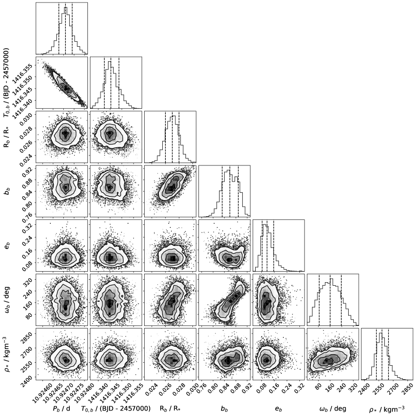
Figure 19: Results of the global photometric fit. This corner plot shows the posterior distributions of the fitted planet parameters for HD 15906 b.

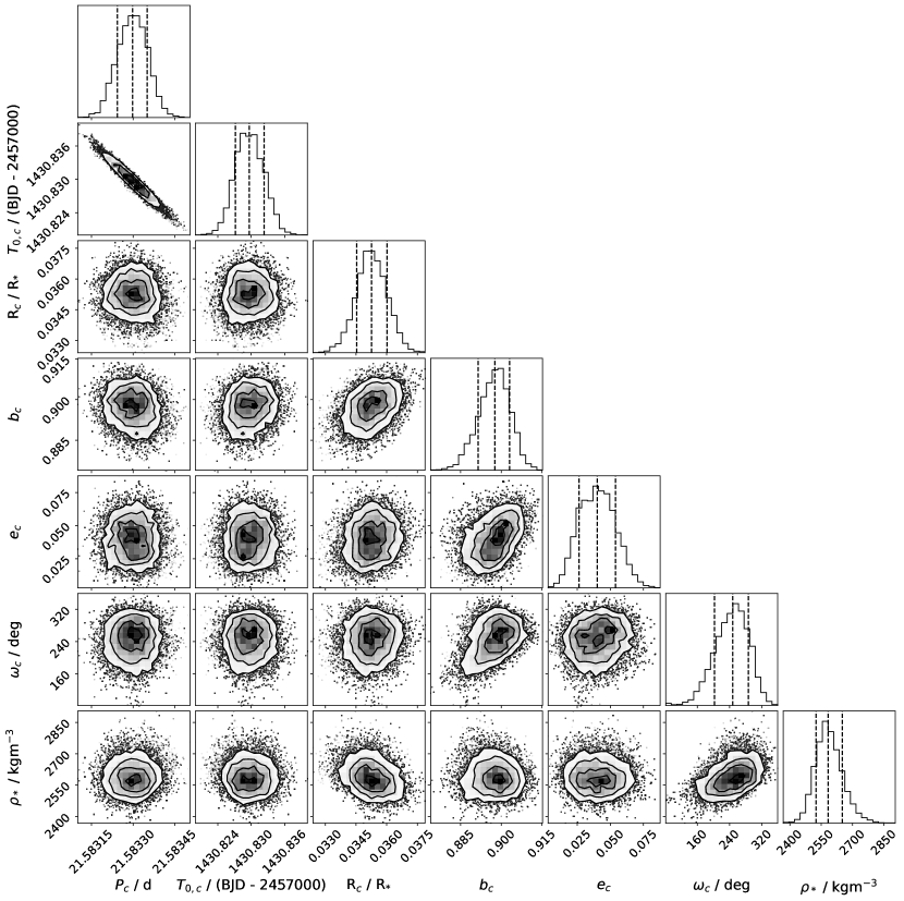
Figure 20: Results of the global photometric fit. This corner plot shows the posterior distributions of the fitted planet parameters for HD 15906 c.

In Table 11, we present the priors and posterior values from the global photometric analysis as described in Section 4.2. In Figures 19 and 20, we present the corner plots of the fitted planet parameters for each planet, made using corner (Foreman-Mackey, 2016).

Table 11: This table presents a full list of the fitted parameters from our global photometric model, described in Section 4.2. We include both the prior and the posterior value of each parameter. Uniform priors are represented by $\mathcal{U}$(a,b) and log-uniform priors are written as ln$\mathcal{U}$(a,b), where a and b are the lower and upper bounds, respectively. The notation used for normal priors is $\mathcal{N}(\mu,\sigma)$, where $\mu$ and $\sigma$ are the mean and standard deviation of the distribution. Truncated normal priors are defined as $\mathcal{N}_{\mathcal{U}}$($\mu$,$\sigma$,a,b), where $\mu$ and $\sigma$ are the mean and standard deviation of the distribution and a and b are the lower and upper bounds, respectively. The limb darkening parameters were defined per instrument (TESS, CHEOPS and LCOGT), however the detrending was done independently for each observation: TESS-1 is the sector 4 data, TESS-2 is the sector 31 data, CHEOPS-1 to -6 are CHEOPS visits 1 to 6 and LCOGT-1 and -2 are LCOGT visits 1 and 2. The posterior values are defined by the median, 16th and 84th percentiles of the posterior distribution.

Parameter	Prior	Posterior Value
HD 15906 b
Period ($P_{\text{b}}$) / days	$\mathcal{U}$(10.92,10.93)	10.924709 $\pm$ 0.000032
Mid-transit time ($T_{0\text{,b}}$) / (BJD - 2457000)	$\mathcal{U}$(1416.3,1416.4)	1416.3453${}^{+0.0034}_{-0.0028}$
Radius ratio (R${}_{\text{b}}$ / R⋆)	$\mathcal{U}$(0.0,0.1)	0.027 $\pm$ 0.001
Impact parameter ($b_{\text{b}}$)	$\mathcal{U}$(0.0,1.2)	0.86 $\pm$ 0.03
Eccentricity ($e_{\text{b}}$)	$\mathcal{N}_{\mathcal{U}}$(0.0,0.083,0.0,1.0)	0.11${}^{+0.04}_{-0.03}$
Argument of periastron ($\omega_{\text{b}}$) / deg	$\mathcal{U}$(0.0,360.0)	160.5${}^{+76.9}_{-75.7}$
HD 15906 c
Period ($P_{\text{c}}$) / days	$\mathcal{U}$(21.58,21.59)	21.583298${}^{+0.000052}_{-0.000055}$
Mid-transit time ($T_{0\text{,c}}$) / (BJD - 2457000)	$\mathcal{U}$(1430.8,1430.9)	1430.8296${}^{+0.0027}_{-0.0025}$
Radius ratio (R${}_{\text{c}}$ / R⋆)	$\mathcal{U}$(0.0,0.1)	0.035 $\pm$ 0.001
Impact parameter ($b_{\text{c}}$)	$\mathcal{U}$(0.0,1.2)	0.90$\pm$ 0.01
Eccentricity ($e_{\text{c}}$)	$\mathcal{N}_{\mathcal{U}}$(0.0,0.083,0.0,1.0)	0.04 $\pm$ 0.01
Argument of periastron ($\omega_{\text{c}}$) / deg	$\mathcal{U}$(0.0, 360.0)	247.9${}^{+38.8}_{-45.4}$
Stellar
Stellar density ($\rho_{\star}$) / kgm-3	$\mathcal{N}$(2517.61,101.94)	2583.24${}^{+68.01}_{-57.80}$
Quadratic LD TESS ($q_{\text{1,{TESS}}}$)	$\mathcal{N}_{\mathcal{U}}$(0.4207,0.1,0.0,1.0)	0.38${}^{+0.04}_{-0.05}$
Quadratic LD TESS ($q_{\text{2,{TESS}}}$)	$\mathcal{N}_{\mathcal{U}}$(0.3659,0.1,0.0,1.0)	0.36${}^{+0.09}_{-0.08}$
Quadratic LD CHEOPS ($q_{\text{1,{CHEOPS}}}$)	$\mathcal{N}_{\mathcal{U}}$(0.5375,0.1,0.0,1.0)	0.54 $\pm$ 0.05
Quadratic LD CHEOPS ($q_{\text{2,{CHEOPS}}}$)	$\mathcal{N}_{\mathcal{U}}$(0.4351,0.1,0.0,1.0)	0.50${}^{+0.06}_{-0.05}$
Quadratic LD LCOGT ($q_{\text{1,LCO}}$)	$\mathcal{N}_{\mathcal{U}}$(0.3442,0.1,0.1,0.0,1.0)	0.39${}^{+0.06}_{-0.05}$
Quadratic LD LCOGT ($q_{\text{2,LCO}}$)	$\mathcal{N}_{\mathcal{U}}$(0.1684,0.1,0.0,1.0)	0.04 $\pm$ 0.04
Instrumental
Flux offset TESS-1 ($\mu_{\text{{TESS}1}}$) / rel. flux	$\mathcal{N}$(0.0,0.1)	0.00020${}^{+0.00049}_{-0.00045}$
Flux offset TESS-2 ($\mu_{\text{{TESS}2}}$) / rel. flux	$\mathcal{N}$(0.0,0.1)	-4.1e-5${}^{+6.7\text{e-}5}_{-7.3\text{e-}5}$
Jitter TESS-1 ($\sigma_{\text{WN,{TESS}1}}$) / ppm	ln$\mathcal{U}$(0.1,1e3)	193.8 $\pm$ 9.0
Jitter TESS-2 ($\sigma_{\text{WN,{TESS}2}}$) / ppm	ln$\mathcal{U}$(0.1,1e3)	193.5${}^{+8.4}_{-8.3}$
M32 GP amplitude TESS-1 ($\sigma_{\text{M32,{TESS}1}}$) / rel. flux	ln$\mathcal{U}$(1e-6,1e6)	0.0012${}^{+0.0004}_{-0.0002}$
M32 GP timescale TESS-1 ($\rho_{\text{M32,{TESS}1}}$) / days	ln$\mathcal{U}$(1e-3,1e3)	2.52${}^{+0.76}_{-0.48}$
SHO GP power TESS-1 ($S_{\text{0,{TESS}1}}$) / (rel. flux)2days	ln$\mathcal{U}$(1e-20,1.0)	3.34e-10${}^{+2.87\text{e-}10}_{-1.40\text{e-}10}$
SHO GP frequency TESS-1 ($\omega_{\text{0,{TESS}1}}$) / days-1	$\mathcal{N}$(28.545,0.1)	28.59${}^{+0.07}_{-0.06}$
SHO GP quality factor TESS-1 ($Q_{\text{{TESS}1}}$)	ln$\mathcal{U}$(0.01,1e4)	0.93${}^{+0.45}_{-0.32}$
M32 GP amplitude TESS-2 ($\sigma_{\text{M32,{TESS}2}}$) / rel. flux	ln$\mathcal{U}$(1e-6,1e6)	32.3e-5${}^{+5.0\text{e-}5}_{-3.7\text{e-}5}$
M32 GP timescale TESS-2 ($\rho_{\text{M32,{TESS}2}}$) / days	ln$\mathcal{U}$(1e-3,1e3)	0.59${}^{+0.13}_{-0.09}$
Flux offset CHEOPS-1 ($\mu_{\text{{CHEOPS}1}}$) / rel. flux	$\mathcal{N}$(0.0,0.1)	5.2e-5 $\pm$ 1.5e-5
Flux offset CHEOPS-2 ($\mu_{\text{{CHEOPS}2}}$) / rel. flux	$\mathcal{N}$(0.0,0.1)	2.2e-5 $\pm$ 1.2e-5
Flux offset CHEOPS-3 ($\mu_{\text{{CHEOPS}3}}$) / rel. flux	$\mathcal{N}$(0.0,0.1)	-10.0e-5 $\pm$ 1.6e-5
Flux offset CHEOPS-4 ($\mu_{\text{{CHEOPS}4}}$) / rel. flux	$\mathcal{N}$(0.0,0.1)	5.3e-5 $\pm$ 1.5e-5
Flux offset CHEOPS-5 ($\mu_{\text{{CHEOPS}5}}$) / rel. flux	$\mathcal{N}$(0.0,0.1)	-6.7e-6 ${}^{+14.9\text{e-}6}_{-14.7\text{e-}6}$
Flux offset CHEOPS-6 ($\mu_{\text{{CHEOPS}6}}$) / rel. flux	$\mathcal{N}$(0.0,0.1)	-10.0e-5${}^{+1.5\text{e-}5}_{-1.4\text{e-}5}$
Jitter CHEOPS-1 ($\sigma_{\text{WN,{CHEOPS}1}}$) / ppm	ln$\mathcal{U}$(0.1,1e3)	138.2${}^{+22.0}_{-21.3}$
Jitter CHEOPS-2 ($\sigma_{\text{WN,{CHEOPS}2}}$) / ppm	ln$\mathcal{U}$(0.1,1e3)	2.7${}^{+20.9}_{-2.3}$
Jitter CHEOPS-3 ($\sigma_{\text{WN,{CHEOPS}3}}$) / ppm	ln$\mathcal{U}$(0.1,1e3)	125.7${}^{+22.9}_{-26.2}$
Jitter CHEOPS-4 ($\sigma_{\text{WN,{CHEOPS}4}}$) / ppm	ln$\mathcal{U}$(0.1,1e3)	128.1${}^{+24.3}_{-26.7}$
Jitter CHEOPS-5 ($\sigma_{\text{WN,{CHEOPS}5}}$) / ppm	ln$\mathcal{U}$(0.1,1e3)	117.2${}^{+20.8}_{-22.1}$
Jitter CHEOPS-6 ($\sigma_{\text{WN,{CHEOPS}6}}$) / ppm	ln$\mathcal{U}$(0.1,1e3)	106.6${}^{+25.4}_{-28.0}$

Table 12: (continued)

Parameter	Prior	Posterior Value
bg detrending coefficient CHEOPS-1	$\mathcal{U}$(-1,1)	11.5e-5 $\pm$ 1.5e-5
t detrending coefficient CHEOPS-1	$\mathcal{U}$(-1,1)	-4.4e-5${}^{+1.5\text{e-}5}_{-1.4\text{e-}5}$
cos($\phi$) detrending coefficient CHEOPS-1	$\mathcal{U}$(-1,1)	-5.6e-5${}^{+1.8\text{e-}5}_{-1.9\text{e-}5}$
x detrending coefficient CHEOPS-2	$\mathcal{U}$(-1,1)	3.0e-5${}^{+1.2\text{e-}5}_{-1.3\text{e-}5}$
y detrending coefficient CHEOPS-2	$\mathcal{U}$(-1,1)	-4.5e-5${}^{+1.2\text{e-}5}_{-1.3\text{e-}5}$
bg detrending coefficient CHEOPS-3	$\mathcal{U}$(-1,1)	5.5e-5 $\pm$ 1.6e-5
x detrending coefficient CHEOPS-3	$\mathcal{U}$(-1,1)	4.9e-5${}^{+1.6\text{e-}5}_{-1.5\text{e-}5}$
y detrending coefficient CHEOPS-3	$\mathcal{U}$(-1,1)	-4.5e-5${}^{+1.4\text{e-}5}_{-1.5\text{e-}5}$
t detrending coefficient CHEOPS-3	$\mathcal{U}$(-1,1)	-3.1e-5 $\pm$ 1.5e-5
cos(3$\phi$) detrending coefficient CHEOPS-3	$\mathcal{U}$(-1,1)	3.9e-5 $\pm$ 2.2e-5
bg detrending coefficient CHEOPS-4	$\mathcal{U}$(-1,1)	5.2e-5 $\pm$ 1.7e-5
y detrending coefficient CHEOPS-4	$\mathcal{U}$(-1,1)	-4.4e-5 $\pm$ 1.4e-5
t detrending coefficient CHEOPS-4	$\mathcal{U}$(-1,1)	12.2e-5${}^{+1.4\text{e-}5}_{-1.3\text{e-}5}$
cos(3$\phi$) detrending coefficient CHEOPS-4	$\mathcal{U}$(-1,1)	6.4e-5${}^{+2.3\text{e-}5}_{-2.2\text{e-}5}$
bg detrending coefficient CHEOPS-5	$\mathcal{U}$(-1,1)	6.6e-5 $\pm$ 1.3e-5
x detrending coefficient CHEOPS-5	$\mathcal{U}$(-1,1)	4.1e-5${}^{+1.1\text{e-}5}_{-1.2\text{e-}5}$
y detrending coefficient CHEOPS-5	$\mathcal{U}$(-1,1)	-5.5e-5 $\pm$ 1.2e-5
t detrending coefficient CHEOPS-5	$\mathcal{U}$(-1,1)	-3.4e-5${}^{+1.2\text{e-}5}_{-1.3\text{e-}5}$
cos(2$\phi$) detrending coefficient CHEOPS-5	$\mathcal{U}$(-1,1)	4.9e-5 $\pm$ 1.7e-5
sin(3$\phi$) detrending coefficient CHEOPS-5	$\mathcal{U}$(-1,1)	-5.5e-5 $\pm$ 1.8e-5
bg detrending coefficient CHEOPS-6	$\mathcal{U}$(-1,1)	3.7e-5${}^{+1.3\text{e-}5}_{-1.4\text{e-}5}$
y detrending coefficient CHEOPS-6	$\mathcal{U}$(-1,1)	-4.8e-5 $\pm$ 1.3e-5
t detrending coefficient CHEOPS-6	$\mathcal{U}$(-1,1)	14.6e-5 $\pm$ 1.3e-5
Flux offset LCOGT-1 ($\mu_{\text{LCO1}}$) / rel. flux	$\mathcal{N}$(0.0,0.1)	2.8e-5 $\pm$ 6.9e-5
Flux offset LCOGT-2 ($\mu_{\text{LCO2}}$) / rel. flux	$\mathcal{N}$(0.0,0.1)	-2.2e-5${}^{+8.4\text{e-}5}_{-8.8\text{e-}5}$
Jitter LCOGT-1 ($\sigma_{\text{WN,LCO1}}$) / ppm	ln$\mathcal{U}$(0.1,1e4)	901.5${}^{+45.4}_{-42.1}$
Jitter LCOGT-2 ($\sigma_{\text{WN,LCO2}}$) / ppm	ln$\mathcal{U}$(0.1,1e4)	901.5${}^{+45.4}_{-42.1}$
airmass detrending coefficient LCOGT-1	$\mathcal{U}$(-1,1)	39.5e-5${}^{+6.4\text{e-}5}_{-6.6\text{e-}5}$
FWHM detrending coefficient LCOGT-1	$\mathcal{U}$(-1,1)	13.7e-5${}^{+6.2\text{e-}5}_{-6.3\text{e-}5}$
airmass detrending coefficient LCOGT-2	$\mathcal{U}$(-1,1)	0.00025${}^{+0.00016}_{-0.00015}$
FWHM detrending coefficient LCOGT-2	$\mathcal{U}$(-1,1)	0.00035 $\pm$ 0.00015

References

- Agol & Fabrycky (2018) Agol E., Fabrycky D. C., 2018, in Deeg H. J., Belmonte J. A., eds, , Handbook of Exoplanets. p. 7, doi:10.1007/978-3-319-55333-7_7
- Almeida-Fernandes & Rocha-Pinto (2018) Almeida-Fernandes F., Rocha-Pinto H. J., 2018, MNRAS, 476, 184
- Barnes (2007) Barnes S. A., 2007, ApJ, 669, 1167
- Barragán et al. (2022) Barragán O., et al., 2022, MNRAS, 514, 1606
- Barros et al. (2022) Barros S. C. C., et al., 2022, A&A, 665, A154
- Bean et al. (2021) Bean J. L., Raymond S. N., Owen J. E., 2021, Journal of Geophysical Research (Planets), 126, e06639
- Benneke et al. (2019) Benneke B., et al., 2019, ApJ, 887, L14
- Benz et al. (2021) Benz W., et al., 2021, Experimental Astronomy, 51, 109
- Blackwell & Shallis (1977) Blackwell D. E., Shallis M. J., 1977, MNRAS, 180, 177
- Bonfanti et al. (2015) Bonfanti A., Ortolani S., Piotto G., Nascimbeni V., 2015, A&A, 575, A18
- Bonfanti et al. (2016) Bonfanti A., Ortolani S., Nascimbeni V., 2016, A&A, 585, A5
- Bonfanti et al. (2021) Bonfanti A., et al., 2021, A&A, 646, A157
- Borsato et al. (2014) Borsato L., Marzari F., Nascimbeni V., Piotto G., Granata V., Bedin L. R., Malavolta L., 2014, A&A, 571, A38
- Borsato et al. (2019) Borsato L., et al., 2019, MNRAS, 484, 3233
- Brown et al. (2013) Brown T. M., et al., 2013, PASP, 125, 1031
- Buchhave et al. (2010) Buchhave L. A., et al., 2010, ApJ, 720, 1118
- Buchschacher et al. (2015) Buchschacher N., Ségransan D., Udry S., Díaz R., 2015, in Taylor A. R., Rosolowsky E., eds, Astronomical Society of the Pacific Conference Series Vol. 495, Astronomical Data Analysis Software an Systems XXIV (ADASS XXIV). p. 7
- Caldwell et al. (2020) Caldwell D. A., et al., 2020, Research Notes of the American Astronomical Society, 4, 201
- Castelli & Kurucz (2003) Castelli F., Kurucz R. L., 2003, in Piskunov N., Weiss W. W., Gray D. F., eds, Vol. 210, Modelling of Stellar Atmospheres. p. A20 (arXiv:astro-ph/0405087)
- Chambers et al. (2016) Chambers K. C., et al., 2016, arXiv e-prints, p. arXiv:1612.05560
- Ciardi et al. (2015) Ciardi D. R., Beichman C. A., Horch E. P., Howell S. B., 2015, ApJ, 805, 16
- Claret (2017) Claret A., 2017, A&A, 600, A30
- Claret (2021) Claret A., 2021, Research Notes of the American Astronomical Society, 5, 13
- Claret & Bloemen (2011) Claret A., Bloemen S., 2011, A&A, 529, A75
- Collier Cameron et al. (2006) Collier Cameron A., et al., 2006, MNRAS, 373, 799
- Collins (2019) Collins K., 2019, in American Astronomical Society Meeting Abstracts #233. p. 140.05
- Collins et al. (2017) Collins K. A., Kielkopf J. F., Stassun K. G., Hessman F. V., 2017, AJ, 153, 77
- Cooke et al. (2019) Cooke B. F., Pollacco D., Bayliss D., 2019, A&A, 631, A83
- Cooke et al. (2020) Cooke B. F., Pollacco D., Lendl M., Kuntzer T., Fortier A., 2020, MNRAS, 494, 736
- Cooke et al. (2021) Cooke B. F., et al., 2021, MNRAS, 500, 5088
- Coughlin et al. (2014) Coughlin J. L., et al., 2014, AJ, 147, 119
- Curtis et al. (2020) Curtis J. L., et al., 2020, ApJ, 904, 140
- Deline et al. (2022) Deline A., et al., 2022, A&A, 659, A74
- Delrez et al. (2021) Delrez L., et al., 2021, Nature Astronomy, 5, 775
- Djupvik & Andersen (2010) Djupvik A. A., Andersen J., 2010, in Highlights of Spanish Astrophysics V. p. 211 (arXiv:0901.4015), doi:10.1007/978-3-642-11250-8_21
- Dragomir et al. (2019) Dragomir D., et al., 2019, ApJ, 875, L7
- Espinoza et al. (2019) Espinoza N., Kossakowski D., Brahm R., 2019, MNRAS, 490, 2262
- Fang & Margot (2012) Fang J., Margot J.-L., 2012, ApJ, 761, 92
- Foreman-Mackey (2016) Foreman-Mackey D., 2016, The Journal of Open Source Software, 1, 24
- Foreman-Mackey et al. (2017) Foreman-Mackey D., Agol E., Ambikasaran S., Angus R., 2017, AJ, 154, 220
- Fressin et al. (2013) Fressin F., et al., 2013, ApJ, 766, 81
- Fulton & Petigura (2018) Fulton B. J., Petigura E. A., 2018, AJ, 156, 264
- Fulton et al. (2017) Fulton B. J., et al., 2017, AJ, 154, 109
- Fulton et al. (2018) Fulton B. J., Petigura E. A., Blunt S., Sinukoff E., 2018, PASP, 130, 044504
- Furlan & Howell (2017) Furlan E., Howell S. B., 2017, AJ, 154, 66
- Furlan & Howell (2020) Furlan E., Howell S. B., 2020, ApJ, 898, 47
- Furlan et al. (2017) Furlan E., et al., 2017, AJ, 153, 71
- Gaia Collaboration et al. (2016) Gaia Collaboration et al., 2016, A&A, 595, A1
- Gaia Collaboration et al. (2022) Gaia Collaboration et al., 2022, arXiv e-prints, p. arXiv:2208.00211
- Gandolfi et al. (2018) Gandolfi D., et al., 2018, A&A, 619, L10
- Garai et al. (2023) Garai Z., et al., 2023, A&A, 674, A44
- Gavel et al. (2014) Gavel D., et al., 2014, in Marchetti E., Close L. M., Vran J.-P., eds, Society of Photo-Optical Instrumentation Engineers (SPIE) Conference Series Vol. 9148, Adaptive Optics Systems IV. p. 914805 (arXiv:1407.8207), doi:10.1117/12.2055256
- Giacalone et al. (2021) Giacalone S., et al., 2021, AJ, 161, 24
- Gibson (2014) Gibson N. P., 2014, MNRAS, 445, 3401
- Gill et al. (2020) Gill S., et al., 2020, ApJ, 898, L11
- Ginzburg et al. (2018) Ginzburg S., Schlichting H. E., Sari R., 2018, MNRAS, 476, 759
- Gomes da Silva et al. (2018) Gomes da Silva J., Figueira P., Santos N., Faria J., 2018, The Journal of Open Source Software, 3, 667
- Gomes da Silva et al. (2021) Gomes da Silva J., et al., 2021, A&A, 646, A77
- Grieves et al. (2022) Grieves N., et al., 2022, A&A, 668, A29
- Guerrero et al. (2021) Guerrero N. M., et al., 2021, ApJS, 254, 39
- Gupta & Schlichting (2019) Gupta A., Schlichting H. E., 2019, MNRAS, 487, 24
- Gupta & Schlichting (2020) Gupta A., Schlichting H. E., 2020, MNRAS, 493, 792
- Guzmán-Mesa et al. (2022) Guzmán-Mesa A., Kitzmann D., Mordasini C., Heng K., 2022, MNRAS, 513, 4015
- Hadden et al. (2019) Hadden S., Barclay T., Payne M. J., Holman M. J., 2019, AJ, 158, 146
- Hoffman & Gelman (2014) Hoffman M. D., Gelman A., 2014, Journal of Machine Learning Research, 15, 1593
- Høg et al. (2000) Høg E., et al., 2000, A&A, 355, L27
- Howell & Furlan (2022) Howell S. B., Furlan E., 2022, Frontiers in Astronomy and Space Sciences, 9, 871163
- Howell et al. (2011) Howell S. B., Everett M. E., Sherry W., Horch E., Ciardi D. R., 2011, AJ, 142, 19
- Hoyer et al. (2020) Hoyer S., Guterman P., Demangeon O., Sousa S. G., Deleuil M., Meunier J. C., Benz W., 2020, A&A, 635, A24
- Ioannidis et al. (2016) Ioannidis P., Huber K. F., Schmitt J. H. M. M., 2016, A&A, 585, A72
- Jenkins (2002) Jenkins J. M., 2002, ApJ, 575, 493
- Jenkins et al. (2010a) Jenkins J. M., et al., 2010a, ApJ, 713, L87
- Jenkins et al. (2010b) Jenkins J. M., et al., 2010b, in Radziwill N. M., Bridger A., eds, Society of Photo-Optical Instrumentation Engineers (SPIE) Conference Series Vol. 7740, Software and Cyberinfrastructure for Astronomy. p. 77400D, doi:10.1117/12.856764
- Jenkins et al. (2016) Jenkins J. M., et al., 2016, in Chiozzi G., Guzman J. C., eds, Society of Photo-Optical Instrumentation Engineers (SPIE) Conference Series Vol. 9913, Software and Cyberinfrastructure for Astronomy IV. p. 99133E, doi:10.1117/12.2233418
- Jenkins et al. (2020) Jenkins J. M., Tenenbaum P., Seader S., Burke C. J., McCauliff S. D., Smith J. C., Twicken J. D., Chandrasekaran H., 2020, Kepler Data Processing Handbook: Transiting Planet Search, Kepler Science Document KSCI-19081-003
- Jensen (2013) Jensen E., 2013, Tapir: A web interface for transit/eclipse observability, Astrophysics Source Code Library (ascl:1306.007)
- Johnson & Soderblom (1987) Johnson D. R. H., Soderblom D. R., 1987, AJ, 93, 864
- Kass & Raftery (1995) Kass R. E., Raftery A. E., 1995, Journal of the American Statistical Association, 90, 773
- Kempton et al. (2018) Kempton E. M. R., et al., 2018, PASP, 130, 114401
- Kipping (2013) Kipping D. M., 2013, MNRAS, 435, 2152
- Kreidberg (2015) Kreidberg L., 2015, Publications of the Astronomical Society of the Pacific, 127, 1161
- Kreidberg et al. (2014) Kreidberg L., et al., 2014, Nature, 505, 69
- Kunimoto & Matthews (2020) Kunimoto M., Matthews J. M., 2020, AJ, 159, 248
- Kupke et al. (2012) Kupke R., et al., 2012, in Ellerbroek B. L., Marchetti E., Véran J.-P., eds, Society of Photo-Optical Instrumentation Engineers (SPIE) Conference Series Vol. 8447, Adaptive Optics Systems III. p. 84473G, doi:10.1117/12.926470
- Kurucz (1993) Kurucz R. L., 1993, SYNTHE spectrum synthesis programs and line data
- Kurucz (2013) Kurucz R. L., 2013, ATLAS12: Opacity sampling model atmosphere program, Astrophysics Source Code Library (ascl:1303.024)
- Lee & Chiang (2016) Lee E. J., Chiang E., 2016, ApJ, 817, 90
- Lee et al. (2014) Lee E. J., Chiang E., Ormel C. W., 2014, ApJ, 797, 95
- Lee et al. (2022) Lee E. J., Karalis A., Thorngren D. P., 2022, ApJ, 941, 186
- Leleu et al. (2021) Leleu A., et al., 2021, A&A, 649, A26
- Li et al. (2019) Li J., Tenenbaum P., Twicken J. D., Burke C. J., Jenkins J. M., Quintana E. V., Rowe J. F., Seader S. E., 2019, PASP, 131, 024506
- Lindegren et al. (2021) Lindegren L., et al., 2021, A&A, 649, A4
- Lissauer et al. (2011) Lissauer J. J., et al., 2011, ApJS, 197, 8
- Lissauer et al. (2012) Lissauer J. J., et al., 2012, ApJ, 750, 112
- Lo Curto et al. (2015) Lo Curto G., et al., 2015, The Messenger, 162, 9
- Lomb (1976) Lomb N. R., 1976, Ap&SS, 39, 447
- Lopez & Rice (2018) Lopez E. D., Rice K., 2018, MNRAS, 479, 5303
- Lozovsky et al. (2018) Lozovsky M., Helled R., Dorn C., Venturini J., 2018, ApJ, 866, 49
- Luque & Pallé (2022) Luque R., Pallé E., 2022, Science, 377, 1211
- Madhusudhan et al. (2014) Madhusudhan N., Amin M. A., Kennedy G. M., 2014, ApJ, 794, L12
- Mamajek & Hillenbrand (2008) Mamajek E. E., Hillenbrand L. A., 2008, ApJ, 687, 1264
- Marcy et al. (2014) Marcy G. W., et al., 2014, ApJS, 210, 20
- Marigo et al. (2017) Marigo P., et al., 2017, ApJ, 835, 77
- Maxted et al. (2021) Maxted P. F. L., et al., 2021, MNRAS,
- Mayor et al. (2003) Mayor M., et al., 2003, The Messenger, 114, 20
- McCully et al. (2018) McCully C., Volgenau N. H., Harbeck D.-R., Lister T. A., Saunders E. S., Turner M. L., Siiverd R. J., Bowman M., 2018, in Proc. SPIE. p. 107070K (arXiv:1811.04163), doi:10.1117/12.2314340
- McGurk et al. (2014) McGurk R., et al., 2014, in Marchetti E., Close L. M., Vran J.-P., eds, Society of Photo-Optical Instrumentation Engineers (SPIE) Conference Series Vol. 9148, Adaptive Optics Systems IV. p. 91483A (arXiv:1407.8205), doi:10.1117/12.2057027
- Monet et al. (2003) Monet D. G., et al., 2003, AJ, 125, 984
- Morris et al. (2020) Morris R. L., Twicken J. D., Smith J. C., Clarke B. D., Jenkins J. M., Bryson S. T., Girouard F., Klaus T. C., 2020, Kepler Data Processing Handbook: Photometric Analysis, Kepler Science Document KSCI-19081-003
- Moses et al. (2013) Moses J. I., et al., 2013, ApJ, 777, 34
- Mugrauer & Michel (2020) Mugrauer M., Michel K.-U., 2020, Astronomische Nachrichten, 341, 996
- Mugrauer & Michel (2021) Mugrauer M., Michel K.-U., 2021, Astronomische Nachrichten, 342, 840
- Nascimbeni et al. (2023) Nascimbeni V., et al., 2023, A&A, 673, A42
- Öberg et al. (2011) Öberg K. I., Murray-Clay R., Bergin E. A., 2011, ApJ, 743, L16
- Orell-Miquel et al. (2022) Orell-Miquel J., et al., 2022, A&A, 659, A55
- Orell-Miquel et al. (2023) Orell-Miquel J., et al., 2023, A&A, 669, A40
- Osborn (2022) Osborn H. P., 2022, MonoTools: Planets of uncertain periods detector and modeler, Astrophysics Source Code Library, record ascl:2204.020 (ascl:2204.020)
- Osborn et al. (2016) Osborn H. P., et al., 2016, MNRAS, 457, 2273
- Osborn et al. (2022) Osborn H. P., et al., 2022, A&A, 664, A156
- Osborn et al. (2023) Osborn H. P., et al., 2023, MNRAS, 523, 3069
- Oshagh et al. (2013) Oshagh M., Santos N. C., Boisse I., Boué G., Montalto M., Dumusque X., Haghighipour N., 2013, A&A, 556, A19
- Otegi et al. (2020) Otegi J. F., Bouchy F., Helled R., 2020, A&A, 634, A43
- Owen & Wu (2013) Owen J. E., Wu Y., 2013, ApJ, 775, 105
- Owen & Wu (2017) Owen J. E., Wu Y., 2017, ApJ, 847, 29
- Persson et al. (2018) Persson C. M., et al., 2018, A&A, 618, A33
- Piskunov & Valenti (2017) Piskunov N., Valenti J. A., 2017, A&A, 597, A16
- Plavchan et al. (2020) Plavchan P., et al., 2020, Nature, 582, 497
- Pollacco et al. (2006) Pollacco D. L., et al., 2006, PASP, 118, 1407
- Rasmussen & Williams (2006) Rasmussen C. E., Williams C. K. I., 2006, Gaussian Processes for Machine Learning
- Ricker et al. (2015) Ricker G. R., et al., 2015, Journal of Astronomical Telescopes, Instruments, and Systems, 1, 014003
- Rogers (2015) Rogers L. A., 2015, ApJ, 801, 41
- Ryabchikova et al. (2015) Ryabchikova T., Piskunov N., Kurucz R. L., Stempels H. C., Heiter U., Pakhomov Y., Barklem P. S., 2015, Phys. Scr., 90, 054005
- Salmon et al. (2021) Salmon S. J. A. J., Van Grootel V., Buldgen G., Dupret M. A., Eggenberger P., 2021, A&A, 646, A7
- Salvatier et al. (2016) Salvatier J., Wiecki T., C. F., 2016, PeerJ Computer Science, 2, e55
- Santos et al. (2013) Santos N. C., et al., 2013, A&A, 556, A150
- Savel et al. (2020) Savel A. B., Dressing C. D., Hirsch L. A., Ciardi D. R., Fleming J. P. C., Giacalone S. A., Mayo A. W., Christiansen J. L., 2020, AJ, 160, 287
- Scargle (1982) Scargle J. D., 1982, ApJ, 263, 835
- Scarsdale et al. (2021) Scarsdale N., et al., 2021, AJ, 162, 215
- Schanche et al. (2020) Schanche N., et al., 2020, MNRAS, 499, 428
- Schlieder et al. (2021) Schlieder J. E., et al., 2021, Frontiers in Astronomy and Space Sciences, 8, 63
- Scott et al. (2021) Scott N. J., et al., 2021, Frontiers in Astronomy and Space Sciences, 8, 138
- Scuflaire et al. (2008) Scuflaire R., Théado S., Montalbán J., Miglio A., Bourge P.-O., Godart M., Thoul A., Noels A., 2008, Ap&SS, 316, 83
- Serrano et al. (2022a) Serrano L. M., et al., 2022a, Nature Astronomy, 6, 736
- Serrano et al. (2022b) Serrano L. M., et al., 2022b, A&A, 667, A1
- Skrutskie et al. (2006) Skrutskie M. F., et al., 2006, AJ, 131, 1163
- Smith et al. (2012) Smith J. C., et al., 2012, PASP, 124, 1000
- Sneden (1973) Sneden C. A., 1973, PhD thesis, THE UNIVERSITY OF TEXAS AT AUSTIN.
- Sousa (2014) Sousa S. G., 2014, [arXiv:1407.5817],
- Sousa et al. (2007) Sousa S. G., Santos N. C., Israelian G., Mayor M., Monteiro M. J. P. F. G., 2007, A&A, 469, 783
- Sousa et al. (2011) Sousa S. G., Santos N. C., Israelian G., Lovis C., Mayor M., Silva P. B., Udry S., 2011, A&A, 526, A99
- Sousa et al. (2015) Sousa S. G., Santos N. C., Adibekyan V., Delgado-Mena E., Israelian G., 2015, A&A, 577, A67
- Sousa et al. (2021) Sousa S. G., et al., 2021, A&A, 656, A53
- Speagle (2020) Speagle J. S., 2020, MNRAS, 493, 3132
- Stassun et al. (2019) Stassun K. G., et al., 2019, AJ, 158, 138
- Stumpe et al. (2012) Stumpe M. C., et al., 2012, PASP, 124, 985
- Stumpe et al. (2014) Stumpe M. C., Smith J. C., Catanzarite J. H., Van Cleve J. E., Jenkins J. M., Twicken J. D., Girouard F. R., 2014, PASP, 126, 100
- Swayne et al. (2021) Swayne M. I., et al., 2021, MNRAS, 506, 306
- Telting et al. (2014) Telting J. H., et al., 2014, Astronomische Nachrichten, 335, 41
- Teske et al. (2020) Teske J., et al., 2020, AJ, 160, 96
- Tokovinin (2018) Tokovinin A., 2018, PASP, 130, 035002
- Trifonov et al. (2020) Trifonov T., Tal-Or L., Zechmeister M., Kaminski A., Zucker S., Mazeh T., 2020, A&A, 636, A74
- Tsiaras et al. (2019) Tsiaras A., Waldmann I. P., Tinetti G., Tennyson J., Yurchenko S. N., 2019, Nature Astronomy, 3, 1086
- Tuson & Queloz (2022) Tuson A., Queloz D., 2022, in Bulletin of the American Astronomical Society. p. 102.205
- Twicken et al. (2010) Twicken J. D., Clarke B. D., Bryson S. T., Tenenbaum P., Wu H., Jenkins J. M., Girouard F., Klaus T. C., 2010, in Software and Cyberinfrastructure for Astronomy. p. 774023, doi:10.1117/12.856790
- Twicken et al. (2018) Twicken J. D., et al., 2018, PASP, 130, 064502
- Ulmer-Moll et al. (2022) Ulmer-Moll S., et al., 2022, A&A, 666, A46
- Ulmer-Moll et al. (2023) Ulmer-Moll S., et al., 2023, A&A, 674, A43
- Valenti & Piskunov (1996) Valenti J. A., Piskunov N., 1996, A&AS, 118, 595
- Van Eylen & Albrecht (2015) Van Eylen V., Albrecht S., 2015, ApJ, 808, 126
- Van Eylen et al. (2018) Van Eylen V., Agentoft C., Lundkvist M. S., Kjeldsen H., Owen J. E., Fulton B. J., Petigura E., Snellen I., 2018, MNRAS, 479, 4786
- Van Eylen et al. (2019) Van Eylen V., et al., 2019, AJ, 157, 61
- Van Eylen et al. (2021) Van Eylen V., et al., 2021, MNRAS, 507, 2154
- Vanderburg et al. (2019) Vanderburg A., et al., 2019, ApJ, 881, L19
- Veras et al. (2011) Veras D., Ford E. B., Payne M. J., 2011, ApJ, 727, 74
- Villanueva et al. (2021) Villanueva S., Dragomir D., Espinoza N., Brahm R., TESS Single Transit Planet Working Group WINE Collaboration 2021, in American Astronomical Society Meeting Abstracts. p. 117.06
- Wang et al. (2015) Wang J., et al., 2015, ApJ, 815, 127
- Weiss et al. (2018) Weiss L. M., et al., 2018, AJ, 155, 48
- Weiss et al. (2022) Weiss L. M., Millholland S. C., Petigura E. A., Adams F. C., Batygin K., Bloch A. M., Mordasini C., 2022, arXiv e-prints, p. arXiv:2203.10076
- Wilson et al. (2022) Wilson T. G., et al., 2022, MNRAS, 511, 1043
- Wizinowich et al. (2000) Wizinowich P., et al., 2000, PASP, 112, 315
- Wright et al. (2010) Wright E. L., et al., 2010, AJ, 140, 1868
- Yıldırım (2022) Yıldırım M. F., 2022, Research in Astronomy and Astrophysics, 22, 055013
- Zechmeister & Kürster (2009) Zechmeister M., Kürster M., 2009, A&A, 496, 577
- Zechmeister et al. (2018) Zechmeister M., et al., 2018, A&A, 609, A12
- Ziegler et al. (2020) Ziegler C., Tokovinin A., Briceño C., Mang J., Law N., Mann A. W., 2020, AJ, 159, 19