STATUS: arXiv pre-print

(1.25in,2in) Fast adaptive high-order integral equation methods for electromagnetic scattering from smooth perfect electric conductors

Felipe Vico
Instituto de Telecomunicaciones y Aplicaciones Multimedia (ITEAM) , Universitat Politècnica de València
felipe.vico@gmail.com

Leslie Greengard
Courant Institute, NYU
New York, NY 10012
and
Center for Computational Mathematics, Flatiron Institute
New York, NY 10010.
greengard@cims.nyu.edu

Michael O’Neil
Courant Institute, NYU
New York, NY 10012
oneil@cims.nyu.edu

Manas Rachh
Center for Computational Mathematics, Flatiron Institute
New York, NY 10010
mrachh@flatironinstitute.org

(1.25in,7.5in)

Abstract

Many integral equation-based methods are available for problems of time-harmonic electromagnetic scattering from perfect electric conductors. Not only are there multiple integral representations that can be used, there are numerous ways in which the geometry can be represented, numerous ways to represent the relevant surface current and/or charge densities, numerous quadrature methods that can be deployed, and numerous fast methods that can be used to accelerate the solution of the large linear systems which arise from discretization. Among the many issues that arise in such scattering calculations are the avoidance of spurious resonances, the applicability of the chosen method to scatterers of non-trivial topology, the robustness of the method when applied to objects with multiscale features, the stability of the method under mesh refinement, the ease of implementation with high-order basis functions, and the behavior of the method as the frequency tends to zero. Since three-dimensional scattering is a challenging, large-scale problem, many of these issues have been historically difficult to investigate. It is only with the advent of fast algorithms and modern iterative methods that a careful study of these issues can be carried out effectively. In this paper, we use GMRES as our iterative solver and the fast multipole method (FMM) as our acceleration scheme in order to investigate some of these questions. In particular, we compare the behavior of the following integral equation formulations with regard to the issues noted above: the standard electric, magnetic, and combined field integral equations (EFIE, MFIE, and CFIE) with standard RWG basis functions [1], the non-resonant charge-current integral equation (NRCCIE) [2], and the decoupled potential integral equation DPIE [3]. Various numerical results are provided to demonstrate the behavior of each of these schemes. Furthermore, we provide some analytical properties and comparisons of the electric charge-current integral equation (ECCIE) [4] and the augmented regularized combined source integral equation (auRCSIE) [5].

Keywords: Electromagnetic (EM) scattering, perfect electric conductor (PEC), second kind integral equation, fast multipole method (FMM), multi-level fast multipole algorithm (MLFMA), high-order adaptive discretization.

1 Introduction

Boundary integral equation methods are widely used in computational electromagnetics (CEM), especially for exterior scattering problems. They impose the outgoing radiation condition exactly and, for piecewise constant homogeneous dielectrics or perfect conductors, reduce the dimensionality of the problem by requiring the discretization of the boundary alone. While the number of degrees of freedom required is dramatically reduced, these methods lead to dense linear systems of equations – hence, fast algorithms are needed to address large-scale problems. At present, state-of-the-art solvers rely on iterative algorithms such as GMRES or BiCGstab. These algorithms work particularly well when the system to be solved is well-conditioned with a spectrum that clusters away from the origin. When computing a solution via an iterative solver, each step requires a matrix-vector product involving the system matrix. There are many algorithms available for accelerating this step, and since it is by now fairly standard in both academic and commercial software, we will rely here on the fast multipole method (FMM) [6, 7, 8, 9, 10]. Iterative solvers with FMM acceleration only require an amount of work on the order of $O(n_{\textrm{iter}}(N\log N))$ for any frequency, where $N$ is the system size and $n_{\textrm{iter}}$ is the total number of iterations.

The focus of the present paper is on the choice of integral formulation, the discretization process, and their effect on performance and accuracy (which can often be dramatic). Currently, the most widely used solvers rely on the electric field, magnetic field, and combined field integral equations (EFIE, MFIE and CFIE) with RWG basis functions and a conforming mesh model of the scatterer [1, 11, 12]. These methods are subject to a host of numerical difficulties, including low-frequency breakdown, high-density mesh breakdown, and standard mathematical ill-conditioning. Rather than changing the underlying formulation, the dominant approach in CEM has been to introduce additional ideas to mitigate these problems. Loop-star basis functions [13, 14, 15, 16], for example, improve accuracy and conditioning in the low-frequency regime. Linear algebraic pre-conditioners [17, 18, 19] alleviate the difficulties produced by the hypersingular integral operator in the EFIE, especially when dense meshes are needed to resolve sub-wavelength features in the geometry. At the same time, there has been a significant effort in the research community to develop well-condtioned Fredholm integral equations of the second kind. While we do not seek to review the literature here, these include the use of Calderon identities to analytically pre-condition the EFIE [20, 21, 18] and the use of regularizing operators to pre-condition the CFIE [22, 23, 24]. A complementary class of methods are the so-called charge-current formulations. These methods are also aimed at developing well-conditioned formulations that are free from low-frequency breakdown [15, 25, 26, 27, 28, 4, 2], but achieve the goal by introducing extra unknowns in the problem. Other formulations that lead to resonance-free, second-kind equations include those based on generalized Debye sources [29, 30] and decoupled potential formulations [3, 31, 32]. More recently an augmented regularized combined source integral equation (auRCSIE) was introduced in [5]. Rather than an exhaustive analysis of all such formulations, we focus here on three representative second-kind integral formulations (NRCCIE, auRCSIE, and DPIE) and use the standard EFIE with RWG basis functions (EFIE-RWG) for comparison.

Once an appropriate second-kind integral formulation has been selected, the accuracy of the obtained solution will depend on the discretization and quadrature methods used. In this paper, we propose and investigate a fast, high-order, adaptive Nyström method that yields high-order convergence and permits adaptive refinement to capture small features in the geometry. Of course, the quality of the geometry description itself also has an impact on the accuracy of the results. Here, we use the method described in [33] which allows for the efficient construction of globally smooth complex surfaces with multiscale features, high-order mesh generation, and local refinement.

With all of this machinery in place, we are able to address challenging electromagnetic scattering problems with millions of degrees of freedom in physically delicate regimes. We show that for the effective solution of such problems, all of the above ingredients play a role in robustly achieving user-specified accuracies in the electric and magnetic fields: well-conditioned formulations, high-order surface representations, and high-order quadratures (complemented by suitable fast algorithms).

2 PEC integral equations with physical unknowns

Electromagnetic scattering from a perfect electric conductor can be studied in the time harmonic regime, where the full Maxwell equations reduce to:

$$\nabla\times\bm{H}^{\operatorname{tot}}=-i\omega\epsilon\bm{E}^{\operatorname{tot}}\,,\quad\nabla\times\bm{E}^{\operatorname{tot}}=i\omega\mu\bm{H}^{\operatorname{tot}}.$$ (2.1)

Here, we assume that the permittivity $\epsilon$ and permeability $\mu$ are scalar constants. The perfect electric conductor (PEC) is defined by a bounded region $\Omega$, possibly with $C$ components $\Omega=\cup_{j=1}^{C}\Omega_{j}$, whose boundary is given by $\Gamma=\partial\Omega$. The boundary of the $j$th component will be denoted $\Gamma_{j}=\partial\Omega_{j}$. As is well-known, the boundary conditions on a PEC are [34, 35]:

$$\bm{n}\times\bm{E}^{\operatorname{tot}} = {\bm{0}},\qquad\bm{n}\cdot\bm{H}^{\operatorname{tot}}=0\,,$$ (2.2)

$$\bm{n}\times\bm{H}^{\operatorname{tot}} = \bm{J},\qquad\bm{n}\cdot\bm{E}^{\operatorname{tot}}=\frac{\rho}{\epsilon}\,,$$

together with the continuity condition along the surface of the scatterer,

$$i\omega\rho=\nabla_{\Gamma}\cdot\bm{J}.$$ (2.3)

It is sufficient to enforce the boundary conditions on the tangential components of the electric field, as done in the EFIE, but one or more of the other (redundant) boundary conditions are often used in the alternative formulations mentioned above and discussed below.

Furthermore, it is convenient to write the total field as the sum of a known incoming field and an unknown scattered field:

$$\bm{E}^{\operatorname{tot}}=\bm{E}^{\operatorname{in}}+\bm{E}^{\operatorname{scat}}\,,\quad\bm{H}^{\operatorname{tot}}=\bm{H}^{\operatorname{in}}+\bm{H}^{\operatorname{scat}}\,.$$ (2.4)

The standard representation for the scattered fields is given in terms of a vector and scalar potential, $\mathbf{A,\phi}$, in the Lorenz gauge:

$$\bm{E}^{\operatorname{scat}} = i\omega\bm{A}^{\operatorname{scat}}-\nabla\phi^{\operatorname{scat}},$$ (2.5)

$$\bm{H}^{\operatorname{scat}} = \frac{1}{\mu}\nabla\times\bm{A}^{\operatorname{scat}},$$ (2.6)

with

$$\bm{A}^{\operatorname{scat}}[\bm{J}](\bm{x})=\mu S_{k}[\bm{J}](\bm{x}),$$ (2.7)

$$\phi^{\operatorname{scat}}[\rho](\bm{x})=\frac{1}{\epsilon}S_{k}[\rho](\bm{x}),$$ (2.8)

and where $\bm{x}\in\mathbb{R}^{3}\setminus\Omega$. The above layer potential operators are defined by

$$S_{k}[\mathbf{a}](\bm{x})=\int_{\Gamma}g_{k}(\bm{x}-\bm{y})\,\mathbf{a}(\bm{y})\,dA_{\bm{y}}\,,$$ (2.9)

$$S_{k}[\sigma](\bm{x})=\int_{\Gamma}g_{k}(\bm{x}-\bm{y})\,\sigma(\bm{y})\,dA_{\bm{y}}\,,$$ (2.10)

with kernel given by the Green’s function

$$g_{k}(\bm{x}-\bm{y})=\frac{e^{ik|\bm{x}-\bm{y}|}}{4\pi|\bm{x}-\bm{y}|}\,.$$ (2.11)

Here, $\mathbf{a}$ is a tangential vector field and $\sigma$ is a scalar on the boundary $\Gamma$. It is important to note that the charge $\rho$ in (2.8) is not an extra degree of freedom, but must satisfy the continuity condition (2.3). This ensures that the resulting electromagnetic fields $\bm{E}^{\operatorname{scat}},\bm{H}^{\operatorname{scat}}$ are Maxwellian.

Using the representation above for the scattered electric and magnetic fields, the EFIE is obtained by imposing the boundary condition $\bm{n}\times\bm{E}^{\operatorname{tot}}={\bm{0}}$, the magnetic field integral equation (MFIE) is obtained by imposing the boundary condition $\bm{n}\times\bm{H}^{\operatorname{tot}}=\bm{J}$, and the standard CFIE is obtained as a linear combination of $\bm{n}\times\bm{H}^{\operatorname{tot}}=\bm{J}$ and $-\bm{n}\times\bm{n}\times\bm{E}^{\operatorname{tot}}={\bm{0}}$. Charge-current formulations, on the other hand, are based on considering the charge term as an independent unknown and imposing another one (or more) of the other conditions in (2.2) in order to obtain a uniquely solvable system of equations [36, 26, 27, 28, 4, 2]. We will often refer to these as augmented formulations, since they have increased the number of unknowns and imposed additional constraints. We turn now to the derivation of one such scheme.

2.1 The Electric Charge-Current Integral Equations

The electric charge-current integral equation (ECCIE) is presented in [4], following the ideas and nomenclature of [26, 37]. It is obtained from the representations (2.5) and (2.6) by imposing the conditions

$$\bm{n}\times\bm{H}^{\operatorname{tot}}=\bm{J},\quad\bm{n}\cdot\bm{E}^{\operatorname{tot}}=\frac{\rho}{\epsilon}\,,$$

yielding

$$\frac{\bm{J}}{2}-M[\bm{J}]=\bm{n}\times\bm{H}^{\operatorname{in}}\\$$ (2.12)

and

$$-i\omega\epsilon\mu\bm{n}\cdot S_{k}[\bm{J}]+\frac{\rho}{2}+S^{\prime}_{k}[\rho]=\epsilon\bm{n}\cdot\bm{E}^{\operatorname{in}}\,,$$ (2.13)

where

$$M[\bm{J}]=\bm{n}\times\nabla\times S_{k}[\bm{J}]\,,$$ (2.14)

is interpreted on surface in the principal value sense, and

$$S^{\prime}_{k}[\rho](\bm{x})=\int_{\Gamma}\frac{\partial g_{k}}{\partial n_{\bm{x}}}(\bm{x}-\bm{y})\,\rho(\bm{y})\,dA_{\bm{y}}.$$ (2.15)

An analogous integral equation known as the Magnetic Charge-Current Integral Equation (MCCIE) can be derived, but it shares similar properties and we will not discuss the formulation in this paper.

2.2 The Non-Resonant Charge-Current Integral Equation

The non-resonant charge-current integral equation (NRCCIE) was introduced in [26, 37], with a modified version in [28]. The basic idea is to make use of (2.12) and (2.13), together with the equation derived from imposing $\bm{n}\cdot\bm{E}^{\operatorname{tot}}=\rho/\epsilon$ and a weak form of the continuity condition (2.3) obtained by integration over the surface. These two equations take the form

$$i\omega\mu\bm{n}\times S_{k}[\bm{J}]-\frac{1}{\epsilon}\bm{n}\times\nabla S_{k}[\rho]=-\bm{n}\times\bm{E}^{\operatorname{in}},$$ (2.16)

$$\nabla\cdot S_{k}[\bm{J}]-i\omega S_{k}[\rho]=0\,.$$ (2.17)

The NRCCIE is a system of two equations, the first obtained as a linear combinations of (2.12) and (2.13), and the second obtained as a linear combinations of (2.16) and (2.17):

$$\frac{\bm{J}}{2}-M[\bm{J}]+\alpha\bm{n}\times\big{\{}i\omega\mu\bm{n}\times S_{k}[\bm{J}]-\frac{1}{\epsilon}\bm{n}\times\nabla S_{k}[\rho]\big{\}} =\bm{n}\times\bm{H}^{\operatorname{in}}-\alpha\bm{n}\times\bm{n}\times\bm{E}^{\operatorname{in}}$$ (2.18)

$$\frac{\rho}{2}+S^{\prime}_{k}[\rho]-i\omega\mu\epsilon\bm{n}\cdot S_{k}[\bm{J}]+\alpha\big{\{}\nabla\cdot S_{k}[\bm{J}]-i\omega S_{k}[\rho]\big{\}} =\epsilon\bm{n}\cdot\bm{E}^{\operatorname{in}}\,.$$

Here, $\alpha$ is an arbitrary real positive constant. The NRCCIE is known to have a unique solution at any frequency $\omega>0$ (see [28]). The operators $\nabla\cdot S_{k}[\bm{J}]$ and $\bm{n}\times\nabla S_{k}[\rho]$ are not compact, however, and therefore the coupled system (2.18) is not strictly speaking a Fredholm equation of the second kind. Nevertheless, we will show that it has similar properties in terms of a small condition number and the absence of high-density mesh breakdown.

3 Augmented Regularized Combined Source Integral Equation

An alternative to the charge-current approach is based on using two tangential vector fields as sources (analogous to using both electric and magnetic current-like variables as unknowns). We focus on the formulation presented in [5], which uses ideas from [22] and [38]. The scheme begins from the following representation for the scattered electric and magnetic fields:

$$\bm{E}^{\operatorname{scat}} =\nabla\times S_{k}[\bm{M}]+i\alpha\nabla\times\nabla\times S_{k}[\bm{J}]$$ (3.1)

$$\bm{H}^{\operatorname{scat}} =i\omega\epsilon\mu S_{k}[\bm{M}]+\nabla\psi+\alpha\omega\epsilon\nabla\times S_{k}[\bm{J}],$$

with

$$\psi =S_{k}[\sigma]+i\beta D_{k}[S_{ik}[\sigma]]$$ (3.2)

$$\bm{J} =\bm{n}\times S_{ik}[\bm{M}],$$

and where $\sigma$ is an unknown scalar and

$$D_{k}[\sigma](\bm{x})=\int_{\Gamma}\frac{\partial g_{k}}{\partial n_{\bm{y}}}(\bm{x}-\bm{y})\,\sigma(\bm{y})\,dA_{\bm{y}}.$$ (3.3)

In the original paper [5], the relation between $\bm{J}$ and $\bm{M}$ was taken to be

$$\bm{J}=\bm{n}\times S^{2}_{ik}[\bm{M}],$$ (3.4)

but the modification above is simpler and more efficient, as there appears to be little difference in conditioning and the number of iterations required for solution.

The corresponding integral equation (auRCSIE) is obtained by imposing the boundary conditions $\bm{n}\times\bm{E}^{\operatorname{tot}}=0$ and $\bm{n}\cdot\bm{H}^{\operatorname{tot}}=0$ along the surface $\Gamma$, yielding:

$$\frac{\bm{M}}{2}+M[\bm{M}]+i\alpha T[\bm{n}\times S_{ik}[\bm{M}]] =-\bm{n}\times\bm{E}^{\operatorname{in}}$$ (3.5)

$$-\frac{\sigma}{2}+S^{\prime}_{k}[\sigma]+i\beta D^{\prime}_{k}[S_{ik}[\sigma]] =b.$$

In the system of equations above, the operator $D^{\prime}_{k}$ is defined by

$$D_{k}^{\prime}[\rho](\bm{x})=\frac{\partial}{\partial n_{\bm{x}}}\int_{\Gamma}\frac{\partial g_{k}}{\partial n_{\bm{y}}}(\bm{x}-\bm{y})\,\rho(\bm{y})\,dA_{\bm{y}},$$ (3.6)

the operator $T$ is defined by

$$T[\bm{J}](\bm{x})=\int_{\Gamma}\bm{n}\times\nabla\times\nabla\times g_{k}(\bm{x}-\bm{y})\,\bm{J}(\bm{y})\,dA_{\bm{y}},$$ (3.7)

and the right hand side $b$ is given by

$$b=-\bm{n}\cdot\bm{H}^{\operatorname{in}}-i\omega\epsilon\mu\bm{n}\cdot S_{k}[\bm{M}]\\ -\alpha\omega\epsilon\bm{n}\cdot\nabla\times S_{k}[\bm{n}\times S_{ik}[\bm{M}]].$$ (3.8)

The auRCSIE system is uniquely solvable for $\omega>0$; it is also uniquely solvable at $\omega=0$ in simply connected geometries. The reader may have noted that no continuity condition was imposed on the unknowns $\bm{M}$ and $\sigma$. It was shown in [5] that the scattered field (3.1) is Maxwellian so long as the right hand side corresponds to a valid incoming Maxwellian electromagnetic field.

4 Decoupled Potential Integral Equation

Instead of solving for the physical quantities, current and charge, one can instead indirectly solve for the vector and scalar potentials themselves. Such an approach leads to the decoupled potential integral equation (DPIE), originally introduced in [3] to address the ubiquitous problem of topological low-frequency breakdown endemic in almost all integral formulations for electromagnetic scattering. The DPIE approach is based on considering two uncoupled boundary value problems: one for the scalar potential, and one for the vector potential. Trivially, both potentials satisfy the homogeneous Helmholtz equation (due to the choice of Lorenz gauge). For the scalar problem, consider the boundary value problem:

$$\Delta\phi^{\operatorname{scat}}+k^{2}\phi^{\operatorname{scat}} =0$$ (4.1)

$$\phi^{\operatorname{scat}}|_{\Gamma_{j}}-V_{j} =-\phi^{\operatorname{in}}|_{\Gamma_{j}}$$

$$\int_{\Gamma_{j}}\frac{\partial\phi^{\operatorname{scat}}}{\partial n}\,ds =-\int_{\Gamma_{j}}\frac{\partial\phi^{\operatorname{in}}}{\partial n}\,ds,$$

where $V_{j}$ is an unknown constant (voltage) assigned to component $j$. And similarly, for the vector potential, consider the boundary value problem:

$$\Delta\bm{A}^{\operatorname{scat}}+k^{2}\bm{A}^{\operatorname{scat}} =0$$ (4.2)

$$\bm{n}\times\bm{A}^{\operatorname{scat}}|_{\Gamma} =-\bm{n}\times\bm{A}^{\operatorname{in}}|_{\Gamma}$$

$$\nabla\cdot\bm{A}^{\operatorname{scat}}|_{\Gamma_{j}}-v_{j} =-\nabla\cdot\bm{A}^{\operatorname{in}}|_{\Gamma_{j}}$$

$$\int_{\Gamma_{j}}\bm{n}\cdot\bm{A}^{\operatorname{scat}}\,ds =-\int_{\Gamma_{j}}\bm{n}\cdot\bm{A}^{\operatorname{in}}\,ds,$$

where, as above, $v_{j}$ is an unknown constant assigned to component $j$. See [3] for a thorough discussion of the role that these constants play in the representation of the fields. Each of these boundary value problems can be solved by means of a second-kind integral equation using the following representations for the scattered scalar and vector potentials:

$$\phi^{\operatorname{scat}}(\bm{x})=D_{k}[\sigma](\bm{x})-i\alpha S_{k}[\sigma](\bm{x}),$$ (4.3)

$$\bm{A}^{\operatorname{scat}}(\bm{x})=\nabla\times S_{k}[\mathbf{a}](\bm{x})-S_{k}[\bm{n}\rho](\bm{x})+i\alpha\big{(}S_{k}[\bm{n}\times\mathbf{a}](\bm{x})+\nabla S_{k}[\rho](\bm{x})\big{)},$$ (4.4)

where we require that $\alpha>0$ (but can be chosen freely), and where

$$D_{k}[\sigma](\bm{x})=\int_{\Gamma}\frac{\partial g_{k}}{\partial n_{\bm{y}}}(\bm{x}-\bm{y})\,\sigma(\bm{y})\,dA_{\bm{y}}$$ (4.5)

is the double layer potential. Imposing the boundary conditions above, and using the fact that $\int_{\Gamma_{j}}D^{\prime}_{0}[\sigma]\,ds=0$, see [3], eq. (A.11), we obtain the following system of equations for the unknowns $\sigma$, $\bm{a}$, $\rho$, the $V_{j}$’s, and the $v_{j}$’s, for $\ell=1,2,\ldots,C$:

$$\frac{\sigma}{2}+D_{k}[\sigma]-i\alpha S_{k}[\sigma]-\sum_{j=1}^{C}V_{j}\chi_{j} =-\phi^{\operatorname{in}}|_{\partial D_{j}},$$ (4.6)

$$\int_{\Gamma_{\ell}}\big{(}(D^{\prime}_{k}-D^{\prime}_{0})[\sigma]+i\alpha\frac{\sigma}{2}-i\alpha S^{\prime}_{k}[\sigma]\big{)}ds =-\int_{\Gamma_{\ell}}\frac{\partial\phi^{\operatorname{in}}}{\partial n}ds\,,$$

$$\frac{1}{2}\left(\begin{array}[]{c}\mathbf{a}\\ \rho\end{array}\right)+\bm{\mathsf{L}}\left(\begin{array}[]{c}\mathbf{a}\\ \rho\end{array}\right)+i\alpha\bm{\mathsf{R}}\left(\begin{array}[]{c}\mathbf{a}\\ \rho\end{array}\right)+\left(\begin{array}[]{c}0\\ \sum_{j=1}^{C}v_{j}\chi_{j}\end{array}\right)=\left(\begin{array}[]{c}-\bm{n}\times\bm{A}^{\operatorname{in}}|_{\Gamma}\\ -\nabla\cdot\bm{A}^{\operatorname{in}}|_{\Gamma_{\ell}}\end{array}\right),$$ (4.7)

$$\int_{\Gamma_{j}}\Big{(}-\bm{n}\cdot S_{k}[\bm{n}\rho]+i\alpha\big{(}\bm{n}\cdot S_{k}[\bm{n}\times\mathbf{a}]\big{)}-i\alpha\left(\frac{\rho}{2}+S^{\prime}_{k}[\rho]\right)\Big{)}ds=-\int_{\Gamma_{j}}\bm{n}\cdot\bm{A}^{\operatorname{in}}\,ds\,,$$ (4.8)

where $\chi_{j}$ is the indicator function such that $\chi_{j}(\bm{x})=1$ if $\bm{x}\in\Gamma_{j}$ and 0 otherwise. The matrix integral operators $\bm{\mathsf{L}}$ and $\bm{\mathsf{R}}$ above are defined by:

$$\bm{\mathsf{L}}\left(\begin{array}[]{c}\mathbf{a}\\ \rho\end{array}\right)= \left(\begin{array}[]{c}L_{11}[\mathbf{a}]+L_{12}[\rho]\\ L_{21}[\mathbf{a}]+L_{22}[\rho]\end{array}\right),\quad$$ (4.9)

where

$$L_{11}[\mathbf{a}]= \hat{\bm{n}}\times S_{k}[\mathbf{a}],$$ (4.10)

$$L_{12}[\rho]= \ -\hat{\bm{n}}\times S_{k}[\hat{\bm{n}}\rho]),$$

$$L_{21}[\mathbf{a}]= \ 0,$$

$$L_{22}[\rho]= \ D_{k}[\rho],$$

and

$$\bm{\mathsf{R}}\left(\begin{array}[]{c}\mathbf{a}\\ \rho\end{array}\right)= \left(\begin{array}[]{c}R_{11}[\mathbf{a}]+R_{12}[\rho]\\ R_{21}[\mathbf{a}]+R_{22}[\rho]\end{array}\right),$$ (4.11)

where

$$R_{11}[\mathbf{a}]= \ \hat{\bm{n}}\times S_{k}[\hat{\bm{n}}\times\mathbf{a}],$$ (4.12)

$$R_{12}[\rho]= \ \hat{\bm{n}}\times\nabla S_{k}[\rho],$$

$$R_{21}[\mathbf{a}]= \ \nabla\cdot S_{k}[\hat{\bm{n}}\times\mathbf{a}],$$

$$R_{22}[\rho]= \ -k^{2}S_{k}[\rho].$$

The vector integral equation above in (4.7) and (4.8) is not, strictly speaking, a Fredholm equation of the second kind since $R_{12}$ and $R_{21}$ are bounded but not compact operators. Nevertheless, we will show that it has similar properties. The formulation is resonance free and stable at arbitrarily low frequencies for geometries of any genus (see [3] for further detail). The original formulation in [3] contains an additional regularizing operator that we have omitted here for simplicity. Stability does not appear to be compromised in our experiments. The coefficient $\alpha$ is included above to avoid spurious resonances; we typically set $\alpha=1$, but for complicated geometries, it may be possible to optimize the choice in order to reduce the total number of iterations.

Remark 1.

If $\alpha=0$, we will refer to the resulting (simpler) integral equation as the resonant DPIE (rDPIE). The spurious resonances are actually the same as those for the MFIE.

5 Properties of various integral formulations

We summarize the expected properties (based on a mathematical analysis) of the various formulations in the table below. We further describe some of the items in the left-hand column of Table 1:

• A spurious resonance is a frequency where the integral equation is not invertible but the scattering problem is itself well-posed.

• High-density mesh breakdown refers to a significant growth in the numerical condition number of the finite-dimensional linear system to be solved under mesh refinement. Some integral equations are Fredholm equations of the second kind which, in the absence of spurious resonances, have bounded condition numbers independent of the number of degrees of freedom.

• Catastrophic cancellation in $\bm{E}^{\operatorname{scat}}$, $\bm{H}^{\operatorname{scat}}$ refers to a loss of precision in computing the scattered fields of interest once the integral equation has been solved (see section 7).

• Second kind integral equations and equations whose system matrices are of the form $I+K$, where $K$ is the discretiztion of a bounded operator, tend to converge rapidly using GMRES or BiCGSTAB as an iterative method.

• An equation is stable at low frequency if the condition number does not grow as the frequency tends to zero. This can be the case for surfaces without holes (of genus zero) or more generally (for surfaces of arbitrary genus).

Table 1: Properties of various integral equation formulations

	EFIE	MFIE	CFIE	ECCIE	NRCCIE	RCSIE	auRCSIE	DPIE
Resonance-free			✓			✓	✓	✓
No high-density mesh breakdown		✓		✓	✓	✓	✓	✓
Second kind Fredholm eq.		✓		✓		✓	✓	✓
Free from catastrophic cancellation in $\bm{E}^{\operatorname{scat}}$, $\bm{H}^{\operatorname{scat}}$				✓	✓		✓	✓
Rapid convergence with GMRES, BiCGSTAB		✓		✓	✓	✓	✓	✓
Stable at low frequencies for surfaces of genus zero		✓		✓	✓	✓	✓	✓
Stable at low frequencies for surfaces of any genus						✓

Following a description of discretization schemes, subsequent sections of the paper provide numerical evidence that the properties summarized above have practical consequences.

6 Surface representation, discretization, and quadrature

Given a flat triangulated surface, it is standard to discretize the EFIE, MFIE or CFIE using edge-based RWG basis functions [1] in a Galerkin framework; this corresponds to linear current profiles on each triangle. Since the formulation is standard, we will not describe it in further detail. We will also investigate the performance of higher-order non-Galerkin discretizations. In this case, we must also assume that the surface $\Gamma$ is described as a set of triangular patches $\Gamma=\cup_{j=1}^{N_{\textrm{patches}}}\Gamma_{j}$, where $N_{\textrm{patches}}$ is the number of curved triangular patches. For each $j$, we assume there exists a known parameterization $\bm{x}_{j}$ such that

$$\bm{x}_{j}:T\rightarrow\Gamma_{j}\subset\mathbb{R}^{3},$$ (6.1)

where $T$ is the canonical unit triangle:

$$T=\big{\{}(u,v):u\geq 0,v\geq 0,u+v\leq 1\big{\}}\,.$$ (6.2)

Remark 2.

Since many computer-aided design systems or meshing algorithms produce only flat triangulations, the surfaces used as examples in this paper are generated using the algorithm of [33]. This results in a surface of the desired form, with the regularity (curvature) of the surface controlled locally, permitting adaptive refinement and resolution of multiscale features.

Given the surface $\Gamma$, described by an atlas of functions $\left\{\bm{x}_{j}\right\}$, we also require a suitable set of sampling/quadrature nodes and a suitable representation of smooth functions on each $\Gamma_{j}$. For this task, we will use Vioreanu-Rokhlin nodes/weights [39], and Koornwinder polynomials as a basis for smooth functions, respectively. The Vioreanu-Rokhlin nodes and weights have been designed so that the quadrature rule

$$\int_{T}f(u,v)\,du\,dv\approx\sum_{i=1}^{p}w_{i}\,f(u_{i},v_{i}),$$ (6.3)

with

$$p=(n_{\textrm{order}}+1)(n_{\textrm{order}}+2)/2$$ (6.4)

nodes exactly integrates all monomials in two variables $u^{k}v^{l}$ whose total order satisfies $k+l\leq n_{\textrm{order}}$. Furthermore, the Koornwinder polynomial $P_{n,m}$ on the standard triangle $T$ are given explicitly by

$$P_{n,m}(u,v)=(1-v)^{m}P^{0,2m+1}_{n-m}(1-2v)\,\,P^{0,0}_{m}\left(\frac{2u}{1-v}-1\right),$$ (6.5)

with $n=0,1,2,...$ and $m=0,1,\ldots,n$. Here $P_{n}^{\alpha,\beta}$ for $n\in\mathbb{N}$ are the standard Jacobi polynomials which are orthogonal with respect to the weight function $(1-x)^{\alpha}(1+x)^{\beta}$ on the interval [-1,1] [40]. This is an orthogonal basis that comes equipped with fast and stable recurrence formulas for their evaluation. Moreover, the mapping from samples of functions at Vioreanu-Rokhlin nodes to the corresponding coefficients in the Koornwinder basis is well-conditioned and straightforward to generate. We refer the reader to [39, 41, 42] for further details. Once the Koornwinder expansion of a function is available, it is a simple matter of evaluation to interpolate that function with high-order accuracy to any other point on the triangle.

Additionally, we also require a basis in which to describe tangential vector fields along each patch. To this end, we construct two sets of vector-valued basis functions on each patch $\Gamma_{j}$ as follows. We first set

$$\bm{u}_{j}(u,v) =\frac{\partial\bm{x}_{j}}{\partial u}$$ (6.6)

$$\bm{n}_{j}(u,v) =\frac{\partial\bm{x}_{j}}{\partial u}\times\frac{\partial\bm{x}_{j}}{\partial v}$$

and

$$\hat{\bm{u}}_{j}(u,v) =\frac{\bm{u}_{j}(u,v)}{|\bm{u}_{j}(u,v)|}$$ (6.7)

$$\hat{\bm{n}}_{j}(u,v) =\frac{\bm{n}_{j}(u,v)}{|\bm{n}_{j}(u,v)|}$$

$$\hat{\bm{v}}_{j}(u,v) =\hat{\bm{n}}_{j}(u,v)\times\hat{\bm{u}}_{j}(u,v).$$

Clearly $\hat{\bm{u}}$, $\hat{\bm{v}}$, $\hat{\bm{n}}$, form a pointwise orthonormal set of coordinates along $\Gamma_{j}$. Then, we set

$$\mathbf{U}^{j}_{n,m}(u,v)=P_{n,m}(u,v)\,\hat{\bm{u}}_{j}(u,v)$$ (6.8)

$$\mathbf{V}^{j}_{n,m}(u,v)=P_{n,m}(u,v)\,\hat{\bm{v}}_{j}(u,v).$$

These vector basis functions are furthermore orthonormal in the sense that

$$\int_{T}\mathbf{U}^{j}_{n,m}(u,v)\cdot\mathbf{U}^{j}_{n^{\prime},m^{\prime}}(u,v)\,du\,dv =\delta_{n,n^{\prime}}\delta_{m,m^{\prime}},$$ (6.9)

$$\int_{T}\mathbf{V}^{j}_{n,m}(u,v)\cdot\mathbf{V}^{j}_{n^{\prime},m^{\prime}}(u,v)\,du\,dv =\delta_{n,n^{\prime}}\delta_{m,m^{\prime}},$$

$$\int_{T}\mathbf{U}^{j}_{n,m}(u,v)\cdot\mathbf{V}^{j}_{n^{\prime},m^{\prime}}(u,v)\,du\,dv =0.$$

In our method, tangential vector fields are represented at each Vioreanu-Rokhlin node $(u_{i},v_{i})$ via an expansion in the two sets of basis functions $\{\mathbf{U}^{j}_{m,n},\mathbf{V}^{j}_{m,n}\}$ (and evaluated at additional points on $\Gamma_{j}$ as needed using the Koornwinder basis).

Remark 3.

The reader may have noted that the basis functions used to discretize tangential vector fields, such as the electric current, do not correspond to a div-conforming discretization. Indeed, no continuity of any kind is enforced between adjacent triangles. This makes discretization very straightforward, as it can be done independently for each triangular patch. As we will see in the numerical examples, this choice does not introduce any artifacts, even at second-order accuracy. The robustness of the method is due to the accuracy of the integration method described below and a fundamental fact about second-kind integral equations: when using Nyström discretizations, the order of accuracy of the method is equal to the order of accuracy of the underlying quadrature scheme [43, 44]. A Nyström method is one in which the integral equation is converted to a finite dimensional linear system by merely sampling the kernel and the unknown at a collection of quadrature nodes and approximating the integral operator by a quadrature rule over those same nodes [45].

6.1 Near and far field quadrature

Since the integral operators appearing in all of our representations are non-local, it is convenient to make use of a quadrature scheme that exploits the smoothness of the integrand when the integral is taken over some triangle $j$ (which we will call the source triangle) and the target point is triangle $i$, with $i\neq j$. Following the discussion in [42], we distinguish the self-interaction (when $i=j$), the near field (when $i\neq j$ but the triangles are adjacent or nearby), and the far field (when $i\neq j$ and the triangles are far apart). For the far field interactions, we use the Vioreanu-Rokhlin quadrature described above (suitable for smooth functions) and for which the fast multipole method FMM [6], [7] can be applied directly to the discrete sum to accelerate the computation. The self interaction is computed by a specialized high-order quadrature rule due to Bremer and Gimbutas [46].

The near interactions correspond to an integrand which is formally smooth but very sharply peaked at the target. These are, in some sense, the most cumbersome integrals to evaluate. For these, we rely on the method introduced in [42], which uses adaptive quadrature on the source triangle $\Gamma_{j}$ with a carefully precomputed multiscale hierarchy of interpolants for the underlying density to reduce the cost. (Although the cost is linear in the total number of degrees of freedom, the accurate evaluation of near field quadratures is the most expensive step in quadrature generation.)

6.2 Error Estimation

The use of orthogonal basis functions to represent the source densities on each triangle has an additional advantage beyond high-order accuracy itself. Namely, these representations can be used for a posteriori error estimation and as a monitor for identifying regions which need further geometric refinement. The procedure is straightforward: from the samples of the unknown densities on each patch, we obtain the coefficients of the corresponding function approximation in the Koornwinder basis. This basis has the property that a well-resolved function has a rapid decay of its Koornwinder coefficients. A basic heuristic for the local error is to simply examine the norm of the highest order basis functions. More precisely, let us first consider a scalar quantity, such as the induced charge $\rho$ on $\Gamma_{j}$. From the discussion above, using the Nyström method, after solving our integral equation we have the discrete values $\rho(\bm{x}_{j}(u_{i},v_{i}))=\rho_{ji}$ at the Vioreanu-Rokhlin nodes. Let us denote the corresponding Koornwinder approximation by:

$$\rho(\bm{x})=\rho(\bm{x}_{j}(u,v))\approx\sum_{m+n\leq n_{\textrm{order}}}c^{j}_{n,m}\,P_{n,m}(u,v).$$ (6.10)

We may then define the following function as our error monitor on this patch:

$$\rho_{\textrm{tail}}(\bm{x}) =\rho_{\textrm{tail}}(\bm{x}_{j}(u,v))$$ (6.11)

$$=\sum_{m+n=n_{\textrm{order}}}c^{j}_{n,m}\,P_{n,m}(u,v)$$

with $L^{2}$ norm

$$\delta\rho_{j}=\sqrt{\int_{\Gamma_{j}}|\rho_{\textrm{tail}}(\bm{x})|^{2}\,dA_{\bm{x}}}$$ (6.12)

which serves as a triangle-by-triangle error estimate. The global absolute and relative errors can then be estimated as

$$\|\delta\rho\|_{2}\approx\sqrt{\int_{\Gamma}|\rho_{\textrm{tail}}(\bm{x})|^{2}dA_{\bm{x}}}$$ (6.13)

and

$$\frac{\|\rho_{\text{error}}\|_{2}}{\|\rho\|_{2}}\approx\sqrt{\frac{\int_{\Gamma}|\rho_{\textrm{tail}}(\bm{x})|^{2}\,dA_{\bm{x}}}{\int_{\Gamma}|\rho(\bm{x})|^{2}\,dA_{\bm{x}}}}\,,$$ (6.14)

respectively. As we will see below, these error estimates are approximately one order of magnitude larger than the error in the radiated field. This is not surprising, since the field quantity is obtained from the density through the process of integration. Note that the $\ell_{2}$ norm of the sequence $\{\delta\rho_{j}\}_{j=1}^{N_{\textrm{patches}}}$ equals $\|\delta\rho\|_{2}$. Plotting the piecewise constant function $\delta\rho_{j}$ on the triangulated surface helps visualize regions with large errors and identifies triangles which require local refinement if the obtained accuracy is not sufficient. The error estimation is analogous for vector densities, such as the electric current.

7 Far Field estimation

The far field induced by a given electric or magnetic current can be computed from the Fourier transform of the currents themselves (see [47]). In some of our formulations, such as the auRCSIE and the DPIE, the unknowns are non-physical quantities. One could develop expressions for the far field in terms of these unknowns using standard parallel-ray approximations. This approach, however, has some disadvantages that we will discuss later. A second option is to use a spherical proxy surface that contains the full scatterer and first compute the corresponding electric and magnetic fields on that sphere. The principle of equivalent currents can then be used to compute the field at any point in the far field (or the far field pattern itself). This latter method has some stability advantages, and is worth describing in more detail.

For known electric and magnetic currents along the proxy sphere $S_{R_{0}}$ of radius $R_{0}$ (with $R_{0}$ sufficiently large so as to enclose the scatterer), the far field pattern is given by:

$$E_{\theta}(\hat{\bm{x}}) =i\frac{e^{ik|\bm{x}|}}{2\lambda|\bm{x}|}\Big{(}\eta N_{\theta}(\hat{\bm{x}})+L_{\phi}(\hat{\bm{x}})\Big{)},$$ (7.1)

$$E_{\phi}(\hat{\bm{x}}) =i\frac{e^{ik|\bm{x}|}}{2\lambda|\bm{x}|}\Big{(}\eta N_{\phi}(\hat{\bm{x}})-L_{\theta}(\hat{\bm{x}})\Big{)},$$

$$H_{\phi}(\hat{\bm{x}}) =\frac{1}{\eta}E_{\theta}(\hat{\bm{x}}),$$

$$H_{\theta}(\hat{\bm{x}}) =-\frac{1}{\eta}E_{\phi}(\hat{\bm{x}}),$$

where

$$\bm{N}(\hat{\bm{x}}) =\int_{S_{R_{0}}}\bm{J}(\bm{y})\,e^{-ik\hat{\bm{x}}\cdot\bm{y}}\,dA_{\bm{y}},$$ (7.2)

$$\bm{L}(\hat{\bm{x}}) =\int_{S_{R_{0}}}\bm{M}(\bm{y})\,e^{-ik\hat{\bm{x}}\cdot\bm{y}}\,dA_{\bm{y}}.$$

The relevant currents can be computed on $S_{R_{0}}$ from the scattered fields $\bm{E},\bm{H}$ (using the FMM for efficiency) according to the equivalent current principle:

$$\bm{J} =\hat{\bm{n}}\times\bm{H},$$ (7.3)

$$\bm{M} =-\hat{\bm{n}}\times\bm{E}.$$

Here $\hat{\bm{n}}$ is the outward unit normal to the sphere $S_{R_{0}}$. If the scatterer is electrically large, the projection integrals in (7.2) are expensive to evaluate naively by direct quadrature over a sufficiently fine mesh on $S_{R_{0}}$. In that case, the fast Fourier transform (FFT) or its non-uniform variant (NUFFT) can be used to accelerate the calculation [48, 49, 50].

Unfortunately, the expressions in (7.2) are unstable at low-frequency and subject to catastrophic cancellation. This problem is discussed in [4] and stems from the fact that the magnitude of the far field is $O(\omega)$ while the integrand is $O(1)$. The stabilization introduced in [4] is based on introducing equivalent electric and magnetic charges. These equivalent charges can easily be obtained from the normal components of the fields $\bm{E}$, $\bm{H}$ on the spherical proxy surface. Numerically stable (and exact) expressions for $\bm{N}$ and $\bm{L}$ are then given by

$$\bm{N}(\hat{\bm{x}}) =\int_{S_{R_{0}}}\left(\bm{J}(\bm{y})(e^{-ik\hat{\bm{x}}\cdot\bm{y}}-1)-i\omega\,\bm{y}\,\rho(\bm{y})\right)dA_{\bm{y}},$$ (7.4)

$$\bm{L}(\hat{\bm{x}}) =\int_{S_{R_{0}}}\left(\bm{M}(\bm{y})(e^{-ik\hat{\bm{x}}\cdot\bm{y}}-1)-i\omega\,\bm{y}\,\sigma(\bm{y})\right)dA_{\bm{y}},$$

where

$$\sigma =\hat{\bm{n}}\cdot\bm{H},$$ (7.5)

$$\rho =\hat{\bm{n}}\cdot\bm{E}.$$

Note that the term $(e^{-ik\hat{\bm{x}}\cdot\bm{y}}-1)$ is also of the order $O(\omega)$ and can be evaluated without catastrophic cancellation as

$$(e^{-ik\hat{\bm{x}}\cdot\bm{y}}-1)=2ie^{i\frac{k}{2}\hat{\bm{x}}\cdot\bm{y}}\sin\left(\frac{k}{2}\hat{\bm{x}}\cdot\bm{y}\right).$$ (7.6)

In short, the expressions in (7.2) are slightly more accurate at high frequencies, while the expressions in (7.4) are significantly more accurate and stable at low frequencies. Thus, we recommend the use of (7.2) for scatterers that are larger than $0.5$ wavelengths in size and (7.4) otherwise.

8 Numerical Examples

In this section, we illustrate the behavior of the integral representations and discretization methods discussed in the preceding sections. For sections 8.1, and 8.2, the scatterer is either a sphere of radius $R=1$m or a smooth version of a rectangular torus, see Figure 1. The toroidal geometry was obtained via the surface smoothing algorithm of [33] applied to a rectangular torus defined as the union of rectangular faces parallel to the coordinate axes.

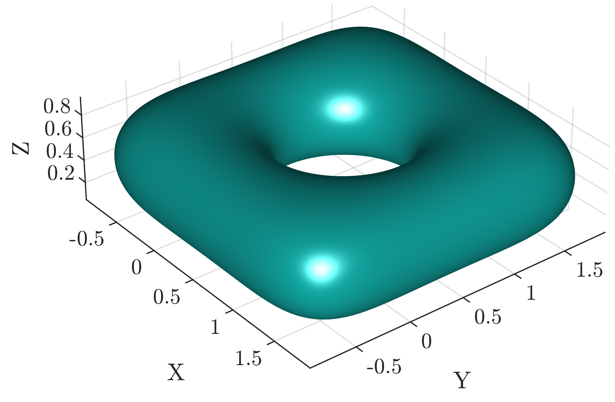
Figure 1: A smoothed rectangular torus of genus one.

The code was implemented in Fortran and compiled using the GNU Fortran 11.2.0 compiler. We use the fast multipole method implementation from the FMM3D package, the high order local quadrature corrections from the fmm3dbie package, and the high-order mesh generation code from the surface smoother package.

In each of the examples, unless stated otherwise, the surface is represented using flat triangles and the integral equations are discretized using a Galerkin approach with the Rao-Wilton-Glisson basis and test functions [1, 51] for the EFIE, MFIE, and CFIE. On the other hand, for the NRCCIE and DPIE, the surface is represented using a collection of high-order curvilinear triangles, and the integral equations are discretized using a Nyström approach with locally-corrected quadratures.

8.1 Accuracy

To test the accuracy of the solvers, we generate an exact solution to the boundary value problem (i.e. the scattering problem) and validate our numerical approximation. Suppose that the boundary data $\bm{E}^{\operatorname{in}}$, $\bm{H}^{\operatorname{in}}$ is generated using a magnetic dipole located in the interior of the perfect electric conductor. Then, the solution in the exterior of the conductor is given exactly by the field due to the magnetic dipole. Let $\varepsilon_{E}$ and $\varepsilon_{H}$ denote the relative $L^{2}$ error in the electric and magnetic fields at a collection of targets in the exterior region, and let $\varepsilon_{a}=\max(\varepsilon_{E},\varepsilon_{H})$. When the conductor is a sphere, we test the accuracy of the computed scattered fields generated by an incident plane wave, where the exact solution in the exterior is given by the Mie series. In a slight abuse of notation, we will use $\varepsilon_{a}$ to denote this error as well.

8.1.1 Convergence

In Figure 2, we plot the error $\varepsilon_{a}$ corresponding to scattering from a PEC sphere with radius $R=$1\text{\,}\mathrm{m}$$ and wavenumber $k=$1\text{\,}\mathrm{m}^{-1}$$ (the diameter of the sphere is $\lambda/\pi$) due to an incoming linearly polarized planewave for each of the EFIE, MFIE, CFIE, NRCCIE, and DPIE; results for the EFIE, MFIE, and CFIE are reported using RWG basis functions, and results for the NRCCIE and DPIE are reported for discretization orders $n_{\textrm{order}}=2,4,6,8$. The errors decrease at the expected rate of $O(h)$ for the EFIE, MFIE, and CFIE, and at the expected rate of $O(h^{n_{\textrm{order}}+1})$ for NRCCIE and DPIE. Here $h$ is the diameter of a typical triangle in the discretization.

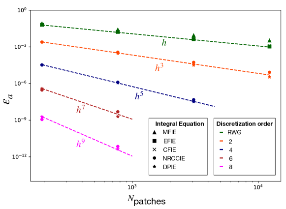
Figure 2: Relative error in the scattered field of a p.e.c. sphere of diameter $D=\frac{1}{\pi}\lambda$ and incoming linearly polarized plane wave. We compare NRCCIE, integral equations with discretization order 2,4,6 and, 8 and the standard CFIE, MFIE, EFIE integral equations discretized with RWG basis functions

8.1.2 Absence of spurious resonances

The exterior scattering problem has a unique solution for any real wavenumber $k$. However, it is well-known that the MFIE has spurious resonances, i.e. wavenumbers $k$ for which the integral equation is not invertible. On the sphere, these spurious resonances can be computed analytically. To demonstrate the absence of spurious resonances for the NRCCIE, and DPIE, we plot the condition number of the discretized integral equations as a function of $k$ in Figure 3. All of the integral equations were discretized using 192 patches and $n_{\textrm{order}}=2$. The interval $k\in[1.9,3.5]$ has one internal resonance of the MFIE on the sphere of radius $R=$1\text{\,}\mathrm{m}$$ given by

$$k_{1} =$2.743\,707\,269\,992\,265\text{\,}\mathrm{m}^{-1}$\,.$$ (8.1)

We observe that all integral equations except the MFIE have a bounded condition number on the range of values of $k$ considered, while the MFIE has a high condition number precisely at its spurious resonant wavenumber. To further confirm the presence of the spurious resonance, we also plot the condition number for the MFIE using $768$ patches and observe that the condition number of the resulting system increases as we obtain a more accurate discretization of the integral equation at the spurious resonance, while there is very little impact on the condition number at the other wavenumbers. When computing the condition numbers of the discretized linear systems, we scale both the unknowns and the boundary data using the square root of the smooth quadrature weights to obtain a better approximation of the integral equation in an $L^{2}$ sense [52].

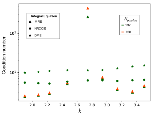
Figure 3: Condition number of the discretized integral equations for the MFIE, NRCCIE, and DPIE.

8.1.3 Static limit

In the static limit, the boundary value problems for the electric and magnetic fields completely decouple. The fields computed at finite, but small wavenumbers, converge to the solutions of the boundary value problems for the electrostatic and magnetostatic fields. Since there exists a stable limit for the underlying system of differential equations, it is a desirable feature that the integral equations remain stable in the static limit as well. Integral equation methods tend to have two kinds of failure modes in the static limit: (1) deterioration in the accuracy of the computed solution using a fixed discretization which resolves both the geometry and the boundary data as $k\to 0$; and (2) failure to converge at the expected rate upon mesh refinement for a fixed, but small $k$.

In Figure 4, we plot the error $\varepsilon_{a}$ as a function of $k$, with $k\in[10^{-10},10^{-1}]$\text{\,}\mathrm{m}^{-1}$$ for the MFIE, EFIE, CFIE, NRCCIE, and DPIE. All of the integral equations were discretized using 192 patches; for the NRCCIE and DPIE we use an $n_{\textrm{order}}=2$ discretization. We note that the CFIE, NRCCIE, and DPIE have no deterioration in accuracy in the limit $k\to 0$, however, for the EFIE, the error increases to $O(1)$ as we decrease $k$. For the MFIE, the error increases like $O(1/k)$ as $k\to 0$.

The nature of the limiting static equations depends on the genus of the conductor and the number of connected components. Thus, the stability of the integral equation may be a function of the topology of the conductor. In Figure 4, we compare the convergence rates for the CFIE, NRCCIE, and DPIE on the smooth torus as we refine the mesh for $k=$1\text{\,}\mathrm{m}^{-1}$$ and $k=10^{-10}$\text{\,}\mathrm{m}^{-1}$$. The error in the computed fields converge at the expected rate for all the integral formulations when $k=$1\text{\,}\mathrm{m}^{-1}$$. On the other hand, for $k=10^{-10}$$\text{\,}\mathrm{m}^{-1}$, the error in the fields computed via the DPIE continues to converge at the expected rate, while the accuracy deteriorates upon mesh refinement for the CFIE and NRCCIE.

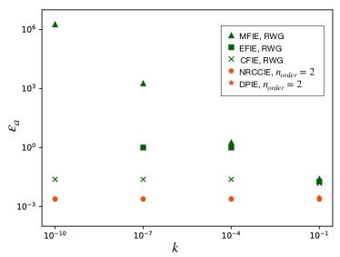
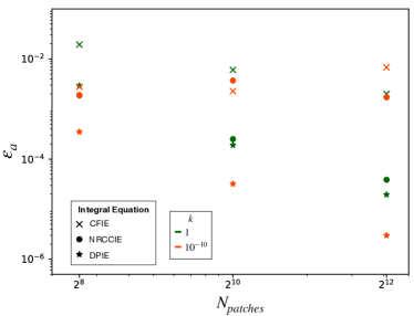
Figure 4: (left) Relative error $\varepsilon_{a}$ as a function of wavenumber $k$ for the MFIE, EFIE, CFIE, NRCCIE, and DPIE on the unit sphere discretized using $N_{\textrm{patches}}=192$, (right) relative error $\varepsilon_{a}$ as a function of number of patches $N_{\textrm{patches}}$ for the CFIE, NRCCIE, and DPIE on a smooth torus with $k=$1\text{\,}\mathrm{m}^{-1}$$ and $k=10^{-10}$\text{\,}\mathrm{m}^{-1}$$.

Remark 4.

For conductors whose dimensions are extremely small compared to the wavelength of the incident field, one could in principle use the solution to the static problems (possibly with including corrections on the Green’s function $g_{k}$ up to $O(k)$) in order to obtain high fidelity approximations of the corresponding low-frequency solutions. Such approximations are widely used in practice, see [53, 54], for example.

8.1.4 A posteriori error estimation

For high-order discretizations, the tail of Koornwinder expansions on each patch can be used as an estimate for the error in the solution computed via integral equations. Following the discussion in Section 6.2, let $\delta J_{j}$ denote the tail of the Koornwinder expansion of the current computed using the NRCCIE and consider the following monitor function

$$\varepsilon_{j}=\delta J_{j}\left(\frac{\|\delta\bm{J}\|_{2}/\|\bm{J}\|_{2}}{\max\limits_{j}\delta J_{j}}\right).$$ (8.2)

The monitor function $\varepsilon_{j}$ is piecewise constant on each triangle, is proportional to $\delta J_{j}$, and its maximum $\|\delta\bm{J}\|_{2}/\|\bm{J}\|_{2}$ is the expected accuracy in the induced current. Typically, the error obtained with the spectral monitor function $\varepsilon_{\rm tail}=\max_{j}\varepsilon_{j}$ is within an order of magnitude of the relative error in the computed scattered field $\varepsilon_{a}$, i.e. $0.1\leq\varepsilon_{a}/\varepsilon_{\rm tail}\leq 10$.

For the NRCCIE on the sphere with wavenumber $k=$1\text{\,}\mathrm{m}^{-1}$$, $N_{\textrm{patches}}=192$, and $n_{\textrm{order}}=4$, the estimated error from the Koornwinder tails of the current is $\varepsilon_{\rm tail}=1.8\times 10^{-4}$, while the error in the field measurements is $\varepsilon_{a}=3.2\times 10^{-5}$. This behavior is independent of the wavenumber, geometry, order of discretization, number of patches used to discretize the conductor, and also holds for other high-order discretizations of second-kind integral equations including, the DPIE. Thus, the error monitor function $\varepsilon_{j}$ can reliably be used to determine adaptive mesh refinement strategies, and $\varepsilon_{\rm tail}$ is a reasonable empirical indicator of the error of the solution on geometries where an analytic solution is not known.

8.2 Iterative solver performance

In this section, we compare the performance of the integral equations when coupled to an iterative solver like GMRES. It is a desirable feature for the GMRES residual to reduce at a rate which is only dependent on the underlying physical problem, e.g. the complexity of the geometry and the boundary data, but independent of the mesh used to discretize the surface. In Figure 5, we plot the relative GMRES residue as a function of the iteration number for the NRCCIE and EFIE. Both the integral equations were discretized with $N_{\textrm{patches}}=192$ and $N_{\textrm{patches}}=768$ patches, and second-order patches were used for discretizing the surface in the NRCCIE. The GMRES residual as a function of iteration number is stable under refinement for the NRCCIE, while for the EFIE, the residual decreases at a slower rate upon mesh refinement. This stability in performance for the NRCCIE can be attributed to its second-kind nature, while the increased number of iterations for the EFIE can be attributed to the hypersingular nature of the EFIE operator — this phenomenon is often referred to as high density mesh breakdown. The iteration count is independent of the discretization order, and number of patches for other second-kind integral equations, such as the DPIE and MFIE, while integral equations with hypersingular kernels like the CFIE also suffer from the high-density mesh breakdown.

Figure 5: Relative GMRES residue for the NRCCIE and the EFIE.

8.3 Speed

In Table 2, we tabulate the total wall time for computing the solution on the PEC sphere with $k=$1\text{\,}\mathrm{m}^{-1}$$ for an incoming linearly polarized plane wave using the NRCCIE and DPIE representations with $(n_{\textrm{order}},\varepsilon_{\textrm{GMRES}})=\{(2,10^{-7}),(4,10^{-9}),(6,10^{-10}),(8,10^{-13})\}$. The wall time, as expected, scales linearly with $N_{\textrm{patches}}$. For each combination of $(n_{\textrm{order}},\varepsilon_{\textrm{GMRES}})$ we note that the total wall time is the smallest for the NRCCIE, followed by the DPIE. The table suggests that for both contractible and non-contractible geometries, away from the static limit, using the NRCCIE would be the optimal choice due to better CPU time performance, while for non-contractible geometries in the static limit, the DPIE is the optimal choice (since the NRCCIE is unstable in that environment). All CPU timings in the table were obtained on a Intel Xeon Gold 6128 Desktop with 24 cores and $192$ GB RAM.

Table 2: Total wall time in seconds for the solution on a PEC sphere at $k=1m^{-1}$ due to an incoming linearly polarized plane wave.

	$n_{\textrm{order}}$	$\epsilon_{\scalebox{0.5}{GMRES}}$	$N_{\textrm{patches}}$
			192	768	3072	12288
NRCCIE	$2$	$10^{\scalebox{0.8}{-7}}$	1.43	7.11	20.7	84.9
	$4$	$10^{\scalebox{0.8}{-9}}$	9.68	28.6	143	-
	$6$	$10^{\scalebox{0.8}{-10}}$	22.9	83.3	-	-
	$8$	$10^{\scalebox{0.8}{-13}}$	63.2	340	-	-
DPIE	$2$	$10^{\scalebox{0.8}{-7}}$	3.18	12.5	48.5	199
	$4$	$10^{\scalebox{0.8}{-9}}$	18.9	64.2	296	-
	$6$	$10^{\scalebox{0.8}{-10}}$	48.1	179	-	-
	$8$	$10^{\scalebox{0.8}{-13}}$	129	594	-	-

8.4 Large-scale examples

We next demonstrate the performance of the integral equations on several large-scale examples. We first demonstrate the efficiency of the DPIE on a multi-genus complicated surface in the static limit, followed by a comparison of the CFIE and NRCCIE for computing the far-field pattern from a bent rectangular cavity. Finally, we illustrate the efficacy of NRCCIE for computing the far-field pattern from a multiscale ship geometry.

8.4.1 High-genus object in the static limit

In the following example, we demonstrate the efficacy and stability of computing the far-field pattern from a genus 17 surface (see Figure 6) in the static limit using the DPIE. None of the other integral equations considered in this manuscript are both numerically and mathematically stable in this regime. The incoming field is a plane wave with wavenumber $k=10^{-10}$\text{\,}\mathrm{m}^{-1}$$. The geometry is contained in a bounding box of size $1.6\times 10^{-10}$ wavelengths in each dimension. As noted in Remark 4, one could, in principle, solve a limiting PDE to obtain a high accuracy approximation of the solution at such low frequencies. However, computing the static solutions requires knowledge of A-cycles and B-cycles on the geometry (i.e. loops through the holes of the surface), which can pose a computational geometry challenge on such complicated high-order surface meshes. The DPIE, on the other hand, can be used directly on the surface triangulation without the need to compute these global loops on the surface.

We first compute a reference solution for this geometry where the surface is discretized with $n_{\textrm{order}}=8$ and $N_{\textrm{patches}}=3840$. In Figure 6, we plot the induced source on the surface of the conductor using this discretization. In order to estimate the accuracy of the computed solution and demonstrate the efficiency of the error monitor function discussed in Section 8.1.4, we also compute the solution using $n_{\textrm{order}}=2$, and $N_{\textrm{patches}}=960$. For this configuration, GMRES required $n_{\textrm{iter}}=72$ for the vector equation and $n_{\textrm{iter}}=21$ for the scalar part for the relative residual to reduce to below $10^{-6}$, and the solution was obtained in 42s. The tolerance for computing the quadrature corrections was $10^{-4}$. The accuracy in the computed far field pattern (as measured in dB) as compared to the far field pattern computed using the reference solution is $1.5\times 10^{-4}$. Another remarkable feature of this calculation is that the DPIE can stably evaluate the far field pattern with values ranging between $[-146,-134]$ dB, which is orders of magnitude smaller than the induced current or the size of the conductor.

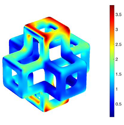
Figure 6: Induced source on the surface of the genus 17 geometry.

8.4.2 Cavity

Next we analyze a cavity in moderately high frequency regime. The rectangular cavity is open at one end, and around $16\lambda$ in length along the center line. The closed end of the cavity cannot be seen from the opening, see Figure 7. The incoming field is a plane wave propagating in the $-\hat{\bm{x}}$ direction and polarized in the $\hat{\bm{z}}$ direction. Due to multiple internal reflections, the physical condition number of the problem is expected to be high, and therefore this problem is a good stress test for high-order methods. The surface of the cavity was discretized using the NRCCIE with $(n_{\textrm{order}},N_{\textrm{patches}})=(2,11392),(4,2848),(4,11392)$, and using the CFIE with $N_{\textrm{patches}}=11392$, and $N_{\textrm{patches}}=45568$. The reference solution for the far field was computed using the NRCCIE with $N_{\textrm{patches}}=11392$ patches of $n_{\textrm{order}}=8$. The estimated error in the reference solution based on the error monitor function $\varepsilon_{\textrm{tail}}=6\times 10^{-5}$. The dominant contributor to the error in the reference solution was the tolerance used for the fast multipole methods and quadrature corrections which was set to $5\times 10^{-7}$. In Figure 7, we plot the magnitude of the induced current computed using the NRCCIE.

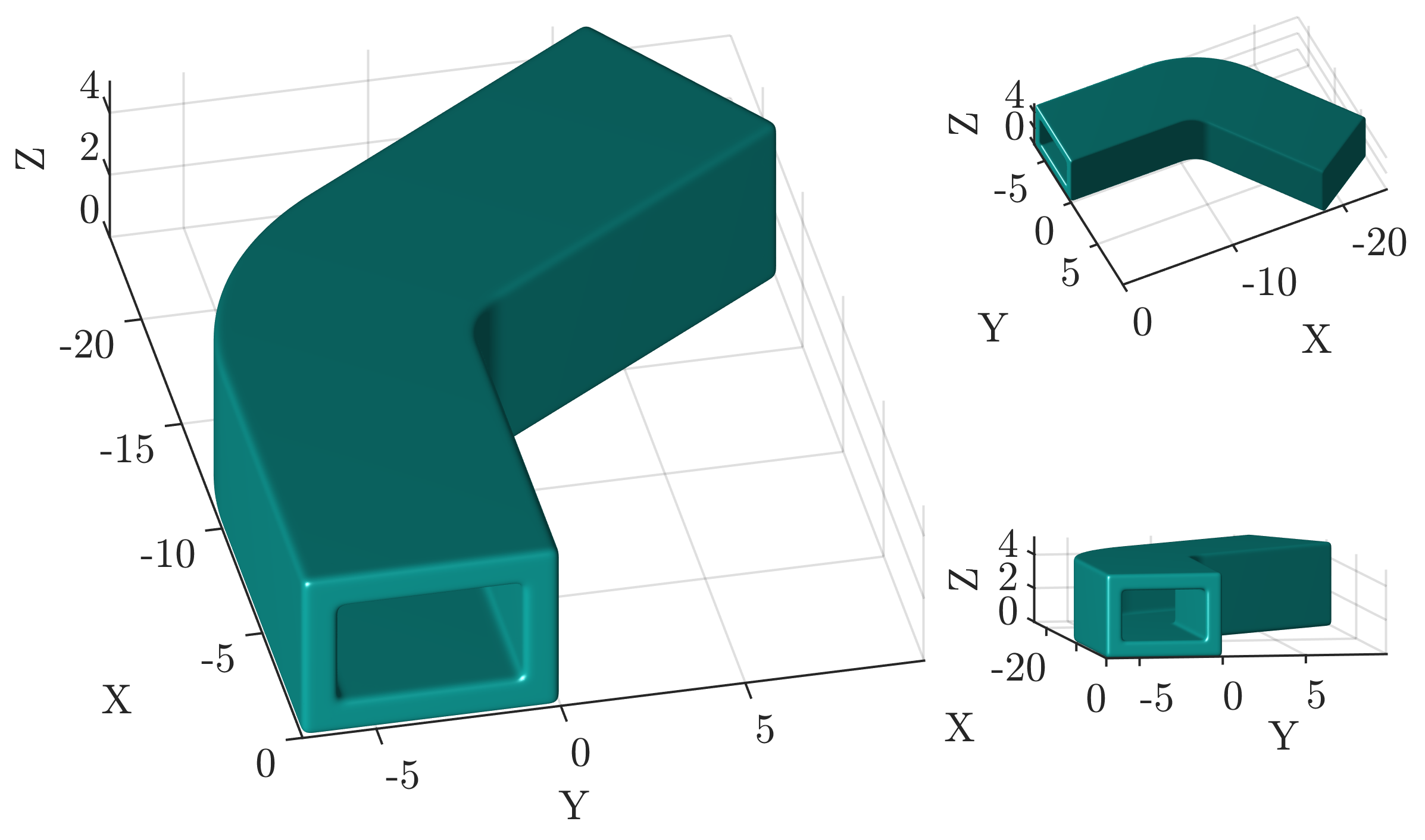
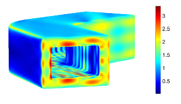
Figure 7: (left) Different views of the cavity, (right) induced current $|\bm{J}|$ for incoming plane wave.

In Table 3, we tabulate the CPU time required to compute the solution ($t_{s}$) and the number of iterations required for the residual to drop below the specified GMRES tolerance $\varepsilon_{\textrm{GMRES}}=10^{-7}$ ($n_{\textrm{iter}}$ ). The precision for computing layer potentials and the FMM was set to $10^{-4}$. We also tabulate the relative $L^{2}$ error in the far field of the electric field denoted by $\varepsilon_{f}$. In Figure 8, we plot the far field $\bm{L}(\theta)=\bm{L}\left(\sin{(\theta)},0,\cos{(\theta)}\right)$ corresponding to the NRCCIE, the CFIE, and the reference solution for $\theta\in[0,180]$ degrees, where $\bm{L}(\hat{\bm{x}})$ is as defined in (7.4).

	$n_{\textrm{order}}$	$N_{\textrm{patches}}$	$n_{\textrm{iter}}$	$t_{s}$	$\varepsilon_{f}$
NRCCIE	$2$	$11392$	$609$	$4.5\times 10^{\scalebox{0.8}{3}}$	$6\times 10^{\scalebox{0.8}{-3}}$
	$4$	$2848$	$607$	$4.0\times 10^{\scalebox{0.8}{3}}$	$5\times 10^{\scalebox{0.8}{-3}}$
	$4$	$11392$	$508$	$7.2\times 10^{\scalebox{0.8}{3}}$	$7\times 10^{\scalebox{0.8}{-4}}$
CFIE	RWG	$11392$	$216$	$2.5\times 10^{\scalebox{0.8}{3}}$	$1\times 10^{\scalebox{0.8}{-1}}$
	RWG	$45568$	$472$	$1.7\times 10^{\scalebox{0.8}{4}}$	$5\times 10^{\scalebox{0.8}{-2}}$

Table 3: Total wall time in seconds, iteration count, and error in far field pattern for the solution on a rectangular cavity of approximately $16$ wavelengths along the center line due to an incoming linearly polarized plane wave.

The table highlights features of the integral equations already observed in the previous sections with respect to linear scaling of the time required to compute the solution for the NRCCIE, the stability of the number of GMRES iterations required for the NRCCIE, and the growth in the number of iterations required for the CFIE. As can be seen from the plots, the error in the far field measurements corresponding to the CFIE with the fine mesh is still $O(1)$, while the far field computed using the fine mesh is nearly indistinguishable from the reference solution. The solution obtained using the NRCCIE can be computed around $4$ times faster than a less accurate solution computed using the CFIE. The table also demonstrates that it is faster and more accurate to use the NRCCIE with $n_{\textrm{order}}=4$ and the coarse mesh as opposed to using NRCCIE with $n_{\textrm{order}}=2$ and the fine mesh.

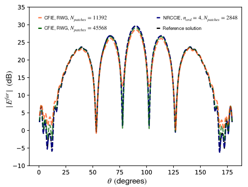
Figure 8: Far field produced by the cavity in Figure 7 for an incoming plane wave.

8.4.3 A multiscale ship simulation

Finally, we demonstrate the performance of NRCCIE on a multiscale ship. The ship is discretized using $N_{\textrm{patches}}=30752$ patches of $n_{\textrm{order}}=4$. The incoming field is a plane wave propagating in the $-\hat{\bm{x}}$ direction and polarized in the $\hat{\bm{z}}$ direction. Let $R_{j}$ denote the radius of the smallest bounding sphere containing patch $\Gamma_{j}$ centered at its centroid. The ratio of the largest to smallest patch size, measured by the enclosing sphere radius $R_{j}$ is $21.5$. The ship is approximately $42\lambda$ in length, $5.7\lambda$ in width, and $8.7\lambda$ in height. The precision for computing the layer potentials and the FMM were set to $10^{-4}$. For this configuration, $289$ GMRES iterations were required for the relative residual to drop below $10^{-6}$, and the solution was computed in $9.1\times 10^{3}$s. The estimated error in the solution is $\varepsilon_{\textrm{tail}}=3.8\times 10^{-3}$. In Figure 9, we plot the absolute value of the induced current on the surface of the ship.

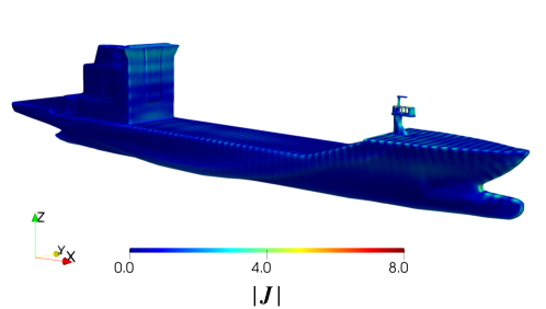
Figure 9: Induced current for incoming plane wave.

9 Conclusions

We have demonstrated the numerical properties of various integral equation methods for solving exterior Maxwell scattering problems, comparing standard RWG discretizations of standard formulations (e.g. EFIE, MFIE, CFIE) to high-order Nyström discretizations of more modern integral formulations especially designed to overcome the failure modes of existing ones (e.g. DPIE, NRCCIE). Furthermore, we’ve shown that when all aspects of the problem are discretized to high-order – the geometry, quadrature, fast algorithm, etc. – that high-order accuracy can be achieved at a cost which is less than that required for lower accuracy using standard 1st-order discretizations. We plan to perform a similar analysis comparing existing integral equation formulations with more modern ones for scattering from piecewise homogeneous dielectric bodies.

References

- [1] S. Rao, D. Wilton, and A. Glisson, “Electromagnetic scattering by surfaces of arbitrary shape,” IEEE Trans. Antennas Propag., vol. 30, no. 3, pp. 409–418, 1982.
- [2] F. Vico, M. Ferrando-Bataller, A. Valero-Nogueira, and A. Berenguer, “A high-order locally corrected nyström scheme for charge-current integral equations,” IEEE Trans. Antennas Propag., vol. 63, no. 4, pp. 1678–1685, 2015.
- [3] F. Vico, M. Ferrando, L. Greengard, and Z. Gimbutas, “The decoupled potential integral equation for time-harmonic electromagnetic scattering,” Comm. Pure Appl. Math., vol. 69, no. 4, pp. 771–812, 2015.
- [4] F. Vico, Z. Gimbutas, L. Greengard, and M. Ferrando-Bataller, “Overcoming low-frequency breakdown of the magnetic field integral equation,” IEEE Trans. Antennas Propag., vol. 61, no. 3, pp. 1285–1290, 2013.
- [5] F. Vico, L. Greengard, M. Ferrando-Bataller, and E. Antonino-Daviu, “An augmented regularized combined source integral equation for nonconforming meshes,” IEEE Trans. Antennas Propag., vol. 67, no. 4, pp. 2513–2521, 2019.
- [6] L. Greengard and V. Rokhlin, “A fast algorithm for particle simulations,” J. Comput. Phys., vol. 73, no. 2, pp. 325–348, 1987.
- [7] L. F. Greengard and J. Huang, “A new version of the fast multipole method for screened coulomb interactions in three dimensions,” Journal of Computational Physics, vol. 180, no. 2, pp. 642–658, 2002.
- [8] V. Rokhlin, “Diagonal forms of translation operators for the helmholtz equation in three dimensions,” Appl. Comput. Harmonic Anal., vol. 1, pp. 82–93, 1993.
- [9] W. Chew, E. Michielssen, J. Song, and J. Jin, Fast and efficient algorithms in computational electromagnetics. Artech House, Inc., 2001.
- [10] H. Cheng, W. Crutchfield, Z. Gimbutas, L. Greengard, J. Ethridge, J. Huang, V. Rokhlin, N. Yarvin, and J. Zhao, “A wideband fast multipole method for the Helmholtz equation in three dimensions,” J. Comput. Phys., vol. 216, no. 1, pp. 300–325, 2006.
- [11] A. Maue, “On the formulation of a general scattering problem by means of an integral equation,” Z. Phys, vol. 126, no. 7, pp. 601–618, 1949.
- [12] J. Mautz and R. Harrington, “H-field, e-field, and combined field solutions for bodies of revolution,” SYRACUSE UNIV NY DEPT OF ELECTRICAL AND COMPUTER ENGINEERING, Tech. Rep., 1977.
- [13] W. Wu, A. Glisson, and D. Kajfez, “A study of two numerical solution procedures for the electric field integral equation at low frequency,” Appl. Comput. Electromagnetics Soc. J., vol. 10, no. 3, pp. 69–80, 1995.
- [14] G. Vecchi, “Loop-star decomposition of basis functions in the discretization of the EFIE,” IEEE Trans. Antennas Propag., vol. 47, no. 2, pp. 339–346, 1999.
- [15] J. Zhao and W. Chew, “Integral equation solution of Maxwell’s equations from zero frequency to microwave frequencies,” IEEE Trans. Antennas Propag., vol. 48, no. 10, pp. 1635–1645, 2000.
- [16] F. Andriulli, K. Cools, I. Bogaert, and E. Michielssen, “On a well-conditioned electric field integral operator for multiply connected geometries,” IEEE Trans. Antennas Propag., vol. 61, no. 4, pp. 2077–2087, 2013.
- [17] K. Sertel and J. Volakis, “Incomplete LU preconditioner for FMM implementation,” Microwave Opt. Tech. Lett., vol. 26, no. 4, pp. 265–267, 2000.
- [18] F. Andriulli, K. Cools, H. Bagci, F. Olyslager, A. Buffa, S. Christiansen, and E. Michielssen, “A multiplicative Calderón preconditioner for the electric field integral equation,” IEEE Trans. Antennas Propag., vol. 56, no. 8, pp. 2398–2412, 2008.
- [19] F. Andriulli and G. Vecchi, “A Helmholtz-stable fast solution of the electric field integral equation,” IEEE Trans. Antennas Propag., vol. 60, no. 5, pp. 2357–2366, 2012.
- [20] S. Christiansen and J. Nedelec, “A preconditioner for the electric field integral equation based on Calderón formulas,” SIAM J. Numer. Anal., vol. 40, no. 3, pp. 1100–1135, 2002.
- [21] H. Contopanagos, B. Dembart, M. Epton, J. Ottusch, V. Rokhlin, J. Visher, and S. Wandzura, “Well-conditioned boundary integral equations for three-dimensional electromagnetic scattering,” IEEE Trans. Antennas Propag., vol. 50, no. 12, pp. 1824–1830, 2002.
- [22] D. Colton and R. Kress, Inverse acoustic and electromagnetic scattering theory. Springer, 2013, vol. 93.
- [23] S. Borel, D. Levadoux, and F. Alouges, “A new well-conditioned integral formulation for maxwell equations in three dimensions,” IEEE Trans. Antennas Propag., vol. 53, no. 9, pp. 2995–3004, 2005.
- [24] O. Bruno, T. Elling, R. Paffenroth, and C. Turc, “Electromagnetic integral equations requiring small numbers of Krylov-subspace iterations,” J. Comput. Phys., vol. 228, no. 17, pp. 6169–6183, 2009.
- [25] Y. Zhang, T. Cui, W. Chew, and J. Zhao, “Magnetic field integral equation at very low frequencies,” IEEE Trans. Antennas Propag., vol. 51, no. 8, pp. 1864–1871, 2003.
- [26] M. Taskinen and P. Yla-Oijala, “Current and charge integral equation formulation,” IEEE Trans. Antennas Propag., vol. 54, no. 1, pp. 58–67, 2006.
- [27] M. Taskinen and D. Vanska, “Current and charge integral equation formulations and Picard’s extended Maxwell system,” IEEE Trans. Antennas Propag., vol. 55, no. 12, pp. 3495–3503, 2007.
- [28] A. Bendali, F. Collino, M. Fares, and B. Steif, “Extension to nonconforming meshes of the combined current and charge integral equation,” IEEE Trans. Antennas Propag., vol. 60, no. 10, pp. 4732–4744, Oct 2012.
- [29] C. Epstein and L. Greengard, “Debye sources and the numerical solution of the time harmonic Maxwell equations,” Comm. Pure Appl. Math., vol. 63, no. 4, pp. 413–463, 2010.
- [30] E. Chernokozhin and A. Boag, “Method of Generalized Debye Sources for the Analysis of Electromagnetic Scattering by Perfectly Conducting Bodies With Piecewise Smooth Boundaries,” IEEE Trans. Antennas Propag., vol. 61, no. 4, pp. 2108–2115, 2013.
- [31] Q. Liu, S. Sun, and W. Chew, “A vector potential integral equation method for electromagnetic scattering,” in Applied Computational Electromagnetics (ACES), 2015 31st International Review of Progress in. IEEE, 2015, pp. 1–2.
- [32] J. Li, X. Fu, and B. Shanker, “Decoupled potential integral equations for electromagnetic scattering from dielectric objects,” IEEE Trans. Antennas Propag., vol. 67, pp. 1729–1739, 2019.
- [33] F. Vico, L. Greengard, M. O’Neil, and M. Rachh, “A fast boundary integral method for high-order multiscale mesh generation,” SIAM J. Sci. Comput., vol. 42, pp. A1380–A1401, 2020.
- [34] J. D. Jackson, Classical Electrodynamics. John Wiley & Sons: New York, 1975.
- [35] C. Papas, Theory of electromagnetic wave propagation. Courier Dover Publications, 1988.
- [36] Z. Qian and W. Chew, “Fast full-wave surface integral equation solver for multiscale structure modeling,” IEEE Transactions on Antennas and Propagation, vol. 57, no. 11, pp. 3594–3601, 2009.
- [37] M. T. P. Yla-Oijala and S. Jarvenpaa, “Advanced surface integral equation methods in computational electromagnetics,” in Electromagnetics in Advanced Applications, 2009. ICEAA’09. International Conference on. IEEE, 2009, pp. 369–372.
- [38] W. Bruno, T. Elling, and C. Turc, “Well-conditioned high-order algorithms for the solution of three-dimensional surface acoustic scattering problems with Neumann boundary conditions,” J. Numer. Meth. Eng, vol. 91, no. 10, 2009.
- [39] B. Vioreanu and V. Rokhlin, “Spectra of multiplication operators as a numerical tool,” SIAM J. Sci. Comput., vol. 36, no. 1, pp. A267–A288, 2014.
- [40] F. W. Olver, D. W. Lozier, R. F. Boisvert, and C. W. Clark, NIST Handbook of Mathematical Functions. Cambridge University Press, 2010.
- [41] T. Koornwinder, “Two-variable analogues of the classical orthogonal polynomials,” in Theory and application of special functions. Elsevier, 1975, pp. 435–495.
- [42] L. Greengard, M. O’Neil, M. Rachh, and F. Vico, “Fast multipole methods for evaluation of layer potentials with locally-corrected quadratures,” J. Comput. Phys.: X, vol. 10, p. 100092, 2021.
- [43] P. M. Anselone, Collectively Compact Operator Approximation Theory and Applications to Integral Equations. Englewood Cliffs, NJ: Prentice-Hall, 1971.
- [44] R. Kress, Linear integral equations. Springer, New York, 2014.
- [45] K. E. Atkinson, The numerical solution of integral equations of the second kind. Cambridge University Press, 1997.
- [46] J. Bremer and Z. Gimbutas, “On the numerical evaluation of the singular integrals of scattering theory,” J. Comput. Phys., vol. 251, pp. 327 – 343, 2013.
- [47] Á. C. Aznar, J. R. Robert, J. M. R. Casals, L. J. Roca, S. B. Boris, and M. F. Bataller, Antenas. Univ. Politèc. de Catalunya, 2004.
- [48] A. Boag, “A fast physical optics (FPO) algorithm for high frequency scattering,” IEEE Trans. Antennas Propag., vol. 52, no. 1, pp. 197–204, 2004.
- [49] L. Greengard and J.-Y. Lee, “Accelerating the non-uniform fast Fourier transform,” SIAM Review, vol. 46, no. 3, pp. 443–454, 2004.
- [50] J.-Y. Lee and L. Greengard, “The type 3 nonuniform fft and its applications,” Journal of Computational Physics, vol. 206, no. 1, pp. 1–5, 2005.
- [51] R. E. Hodges and Y. Rahmat-Samii, “The evaluation of MFIE integrals with the use of vector triangle basis functions,” Microwave Opt. Tech. Lett., vol. 14, no. 1, pp. 9–14, 1997.
- [52] J. Bremer and Z. Gimbutas, “On the numerical evaluation of the singular integrals of scattering theory,” Journal of Computational Physics, vol. 251, pp. 327–343, 2013.
- [53] E. Haber and S. Heldmann, “An octree multigrid method for quasi-static Maxwell’s equations with highly discontinuous coefficients,” J. Comput. Phys., vol. 223, no. 2, pp. 783–796, 2007.
- [54] S. Kapur and D. E. Long, “IES3: A fast integral equation solver for efficient 3-dimensional extraction,” in Proceedings of IEEE International Conference on Computer Aided Design, vol. 97, 1997, pp. 448–455.