Scalable and Exponential Quantum Error Mitigation of BQP Computations using Verification

Abstract

We present a scalable and modular error mitigation protocol for running $\mathsf{BQP}$ computations on a quantum computer with time-dependent noise. Utilising existing tools from quantum verification, our framework interleaves standard computation rounds alongside test rounds for error-detection and inherits a local-correctness guarantee which exponentially bounds (in the number of circuit runs) the probability that a returned classical output is correct. On top of the verification work, we introduce a post-selection technique we call basketing to address time-dependent noise behaviours and reduce overhead. The result is a first-of-its-kind error mitigation protocol which is exponentially effective and requires minimal noise assumptions, making it straightforwardly implementable on existing, NISQ devices and scalable to future, larger ones.

I Introduction

Quantum error mitigation (QEM) [1, 2, 3, 4, 5] broadly refers to the class of techniques designed to deal with errors on near-term quantum computers where the number of accessible qubits is too low to enable quantum error correction. Such techniques typically attempt to mitigate errors by running the same circuit a large number of times on a noisy device and performing some classical post-analysis, for example calculating an empirical estimate of an expectation value using zero-noise Richardson extrapolation [6, 7, 8, 9] or ‘averaging out’ errors using probabilistic error cancellation [3, 7, 10, 11, 12] or virtual distillation [13, 14, 15, 16, 17].

However, QEM is typically limited in its capacity to scale with increasing qubit numbers and circuit depths due to the necessity to adopt a noise model such that the underlying theory becomes tractable [5, 18]. These noise models are typically either oversimplified and unscalable in practice or instead require an exponentially scaling classical description, all while suffering from a trade-off between quantities such as bias and variance [19]. Hence, as near-term devices scale in complexity, these techniques will become obsolete and new approaches will be required which are robust enough to address errors on both near and intermediate-term devices.

In this paper, we consider computations from the $\mathsf{BQP}$ complexity class, which can broadly be viewed as polynomially-sized decision problems with a single-bit output. A straightforward way to perform error mitigation on $\mathsf{BQP}$ computations is to run the same computation many times and to take a majority vote on the obtained single-bit outcomes. If we can bound the probability of obtaining the incorrect result below $\frac{1}{2}$, this procedure will exponentially mitigate the probability of error in the number of circuit runs.

However, one cannot confidently bound this probability below $\frac{1}{2}$ in general. Since the correct result of the $\mathsf{BQP}$ computation is unknown to the user, they cannot gauge how erroneously their quantum computer is behaving. Additionally, and especially on noisy intermediate-scale quantum (NISQ) devices, the device noise may fluctuate such that there only exist certain times when the noise is sufficiently low to enable an error rate below $\frac{1}{2}$.

Our work is to show that we can still obtain exponential error mitigation in this case. To do so, we inherit several ideas from an existing quantum verification protocol [20]. Verification refers to the situation in which we want to run a quantum computation on a remote device that we do not trust, and has been used to inspire error mitigation techniques before [21]. In this case, runs of the standard $\mathsf{BQP}$ computation are interleaved with ‘test rounds’ which are used for error detection. In particular, we obtain a local-correctness property which exponentially bounds (in the total number of circuit runs) the probability that a single-bit decision accepted by our error mitigation protocol is the correct result of the $\mathsf{BQP}$ computation. Additionally, we obtain noise-robustness in that there is no requirement to adopt any particular noise model or device tomography, beyond some basic assumptions on how the noise changes with time. This enables our error mitigation protocol to be straightforwardly applied on a wide range of existing NISQ devices, and to scale with increasing future hardware complexity.

We then build upon this work to reduce its sensitivity to high or fluctuating noise levels by introducing a post-selection technique which we call basketing, whereby the noise is regularly sampled and batches of runs deemed too noisy are discarded and repeated. This would not be permitted in a verification setting where the quantum device is untrusted due to its potential to leak information about the performed test and computation rounds, but can be performed in the context of error mitigation on a trusted device under some basic noise assumptions. Our basketing technique also enables the protocol to be run in parallel across multiple QPUs/clusters at once, meaning the overhead can be spread across both time and space.

We present our error mitigation protocol in a modular way. We first give separate subroutines for running the test and computation rounds. We also state a resource estimation procedure, enabling the user to specify some required target accuracy and receive optimal values of parameters for running the protocol. Finally we state our basketing protocol, detailing how to use the above subroutines to achieve exponential error mitigation for $\mathsf{BQP}$ computations. This work is presented using measurement-based quantum computation (MBQC); we hence also outline a subroutine which enables our work to run on devices using the circuit model, provided such a device supports mid-circuit measurements in the standard basis and the ability to condition future gates on these measurement outcomes. Since we are not working in a security setting, our modular approach allows for much of the mathematical heavy-lifting to be condensed solely into the resource estimation procedure with the intention of making our work easily accessible and implementable by the wider community.

Finally, we demonstrate our protocol using classical simulation. We show that our basketing technique is able to alleviate the noise-sensitivity bottleneck of the underlying verification work in time-dependent noise scenarios whilst in some cases dramatically reducing the required overhead of circuit runs.

We anticipate that a future update to this work will enable the use of test rounds which are tailored to specific applications or device architectures; our modular approach makes it straightforward to implement such improvements within a general framework for error mitigation protocols. In addition, the underlying ‘trappification’-based verification work is being developed to consider general (not necessarily $\mathsf{BQP}$) computations and hence in the future our error mitigation framework may be able to treat general computations outside of the $\mathsf{BQP}$ class as well.

II Background theory

II.0.1 $\mathsf{BQP}$ computations

Our protocol considers computations in the bounded-error quantum polynomial time ($\mathsf{BQP}$) complexity class [22]. We say a language $L$ is in $\mathsf{BQP}$ if there exists a family of polynomially-sized quantum circuits, $\{Q_{n}:n\in\mathbb{N}\}$ such that:

• for all $n\in\mathbb{N}$, $Q_{n}:\{0,1\}^{n}\rightarrow\{0,1\}$ maps an $n$-bit input to a 1-bit output;

• for all $x\in L,|x|=n,\ \mathbb{P}(Q_{n}(x)=1)\geq\frac{2}{3}$;

• for all $x\notin L,|x|=n,\ \mathbb{P}(Q_{n}(x)=0)\geq\frac{2}{3}$,

where $\mathbb{P}(A)$ denotes the probability of an event $A$ occurring and $|x|$ denotes the number of bits in $x$. Hence, each $\mathsf{BQP}$ computation comes with an inherent error probability $p$, and consequentially each run of a $\mathsf{BQP}$ computation for a given classical input string $x$ corresponds to a non-deterministic evaluation of $Q_{|x|}(x)=0$ or 1, which we call the decision function. Since $p<\frac{1}{2}$ in a noiseless scenario, we can hence estimate with exponential confidence whether $x\in L$ by evaluating $Q_{|x|}(x)$ a large number of times and taking a majority vote over the obtained outcomes.

In this paper, we consider the implementation of a general $\mathsf{BQP}$ computation with classical input $x$ as the relevant quantum computation with quantum input $\ket{x}\mapsto U\ket{x}$ followed by computational basis measurements to produce some classical output string $c_{x}$. Classical post-processing then applies some known mapping $c_{x}\mapsto Q_{|x|}(x)$ to infer the value of the decision function based on the measured computation outcome.

II.0.2 Measurement-Based Quantum Computing (MBQC)

We describe the key details of the MBQC framework in which our protocol is written. Readers requiring a more detailed explanation of MBQC are referred to, for example, reference [23]. In Section III, we sketch a subroutine for implementing our work in the circuit model.

Measurement-based quantum computing provides an alternative universal framework to the circuit model for running quantum computations. Computations are defined using a graph $G=(V,E)$ where $V$ and $E$ are the sets of vertices and edges. The vertices correspond to qubits; we define two vertex subsets $I,O\subseteq V$ which denote the input and output qubits of the computation. We also define a list of angles $\{\phi_{v}\}_{v\in V}$ where the angles are quantised via $\phi_{v}\in\Theta\equiv\{k\pi/4\}_{k=0}^{7}$. The graph also has an associated flow which dictates an ordering of the vertices – see for example [24] for a detailed description. We typically collate this data and call it a pattern $\mathcal{P}$.

We consider for now MBQC computations within a Client-Server scenario, where a Client (able to perform classical computations) has access to a remote Server (able to perform classical and quantum computations) via some classical channel. We assume that both the Client and Server are noise-free and that the Server is trusted by the Client. We will explain later modifications which enable these assumptions on the Server to be removed for verification and error mitigation.

A computation is then performed in the following way. The Client first gives the Server the classical details of the pattern $\mathcal{P}$ corresponding to the computation. The Server then initialises the graph state,

$$\ket{G}=\prod_{(i,j)\in E}\textbf{CZ}_{ij}\ \bigotimes_{v\in V}\ket{+}.$$ (1)

This is achieved by first preparing each vertex of the graph in the $\ket{+}=\frac{1}{\sqrt{2}}\left(\ket{0}+\ket{1}\right)$ state, before applying a controlled-$Z$ (CZ) gate between every pair of vertices with an edge between them in the graph. For computations with a quantum input, the state $\bigotimes_{v\in I}\ket{\psi_{v}}$ may be specified by the Client to be some separate input state – for $\mathsf{BQP}$ computations, this is typically the state $\bigotimes_{i=1}^{|x|}\ket{x_{i}}_{i}$ where $x=(x_{i})_{i=1}^{|x|}$ is the classical input to the computation.

Finally, the Client asks the Server to measure each qubit of $V$ in an order dictated by the flow of the graph. Each qubit with corresponding vertex $v$ is measured with respect to the basis $M_{XY}(\phi_{v}^{\prime})$, where $M_{XY}(\theta)=\{\ket{+_{\theta}},\ket{-_{\theta}}\}$ with $\ket{\pm_{\theta}}=\frac{1}{\sqrt{2}}\left(\ket{0}+e^{i\theta}\ket{1}\right)$. The angles $\phi_{v}^{\prime}$ are corrected angles given by $\phi_{v}^{\prime}=(-1)^{s_{v}^{X}}\phi_{v}+s_{v}^{Z}\pi$ where $s_{v}^{X},s_{v}^{Z}\in\{0,1\}$ are dependent on the outcomes of previously measured qubits and the flow.

II.0.3 Verification protocol for $\mathsf{BQP}$ computations

We now describe the theory from the verification of $\mathsf{BQP}$ computations that our work inherits.

In the previous subsection, we introduced measurement-based quantum computation under the scenario in which a Client interacts with a Server that is assumed to be both noise-free and trusted. Naturally, any near- to intermediate-term commercial use of a remote quantum computer will need to relax both of these assumptions such that computations are noise robust, private and secure against a potentially malicious Server. Running a quantum computation on a Server under these requirements demands the use of a quantum verification protocol – several such protocols and frameworks have been developed [25, 26, 27, 28, 29, 30].

Our work is an adaptation of an existing verification protocol given in [20]. This work considers the scenario of a trusted, noiseless Client (verifier) interacting with an untrusted, noisy Server (prover) using the measurement-based quantum computing framework. The framework also assumes that the Client is able to noiselessly prepare qubits and send them to the Server via a quantum channel – for our error mitigation purposes, these assumptions can be replaced simply with a noise-independence assumption between state preparation and computation, allowing us to view the Client and Server as a single entity. For now, we keep the formalism of the original framework intact to be able to clearly identify the assumptions made.

We now describe the general strategy employed by this verification protocol, stating in Theorem 1 how this protocol leads to exponential convergence around the correct classical outcome. The verification protocol is defined by interleaving standard computation rounds (i.e. individual runs of the target $\mathsf{BQP}$ computation on our quantum Server) alongside test rounds, which are used as an error-detection mechanism to gauge whether the Server is corrupting the computation – either maliciously or due to the inherent noise of the underlying device. The test rounds are constructed in such a way that, from the point of view of the Server, they cannot be distinguished from the standard computation rounds – this obfuscation is achieved by applying the Universal Blind Quantum Computing protocol [31] to each test and computation round. This forces a malicious Server – one which is trying to corrupt and/or learn the details of our computations – to have a high probability of corrupting some proportion $\varphi$ of the test rounds; the Client can then detect these deviations using classical post-processing on the obtained measurement results.

To run the protocol, some uniformly random ordering of $t$ test rounds and $d$ computation rounds is selected by the Client, who instructs the Server to run them according to that order. The test rounds are recorded by the Client to either pass or fail, based on their measurement outcomes satisfying some efficiently-computable classical condition, whilst the computation rounds return a classical outcome, corresponding (in the ideal case) to the output $Q_{|x|}(x)\in\{0,1\}$ of the decision function for the target $\mathsf{BQP}$ computation (see Section II.0.1).

If the proportion of corrupted test rounds is at least that of some threshold proportion $\Phi$, dictated at the beginning of the protocol, then the protocol aborts. If not, the protocol takes a majority vote on the decision function values $Q_{|x|}(x)\in\{0,1\}$ obtained from the computation rounds, which are then shown in Theorem 1 to exponentially concentrate on the correct result.

We emphasise here that the strength of this error-detection mechanism is derived in essence from the use of the Universal Blind Quantum Computing protocol [31] that enables us to hide our computations, requiring only for each qubit of the computation to be randomised by the Client. This is highly comparable to many randomised benchmarking techniques in which a random Clifford circuit is exploited to impose some depolarisation of the error channel. Unlike randomised benchmarking, however, only local Pauli operations are required to achieve this randomness and in this case we obtain exponentially scaling confidence in the exact outcome of the target computation. The UBQC protocol is indirectly implemented via the steps of Subroutines 1 and 2 for running the computation and test rounds, and hence the aforementioned benefits are later inherited by our error mitigation protocol.

We will see later via classical simulation that a noticeable drawback of this verification protocol within an error mitigation setting is its sensitivity to fluctuating noise. Due to its security constraints, post-selection is largely prohibited and hence minor perturbations in the noise level can be viewed as malicious and can cause the protocol to abort. In addition, too high a noise level can prevent the protocol from being able to run at all. We address these issues later using our basketing technique.

Finally, we state the central theoretical result which our protocol utilises, placing exponential confidence on any accepted classical result using local-correctness. We first define local-correctness using the idea of a two-party protocol, as set out in the Appendix of [20].

Subroutine 1.

Computation round Client’s inputs: A $\mathsf{BQP}$ computation with corresponding MBQC pattern $\mathcal{P}$ as defined in Section II.0.2 and classical input $x=(x_{i})_{i=1}^{|I|}$; a function $q:\{0,1\}^{|O|}\xrightarrow{}\{0,1\}$ mapping the computation outputs to the corresponding output of the decision function. Subroutine steps: 1. For each qubit with vertex $v\in V$, the Client chooses at random $\theta_{v}\in\Theta$ and prepares the state $\ket{+_{\theta_{v}}}$. The Client may also prepare $\bigotimes_{v\in I}\ket{\psi_{v}}$ to be the quantum input to the computation. 2. The Client sends the $|V|$ many prepared qubits to the Server. 3. The Client instructs the Server to prepare the graph state by performing a $\mathbf{CZ}_{ij}$ gate between all pairs of qubits $i,j$ with $(i,j)\in E$. 4. For each qubit $v\in V$, in the order dictated by the flow $f$: (a) The Client picks a uniformly random bit $r_{v}\in\{0,1\}$ and instructs the Server to measure the qubit at angle $\delta_{v}=\phi_{v}^{\prime}+\theta_{v}+r_{v}\pi$, where $\phi_{v}^{\prime}$ is the standard corrected angle as described in Section II.0.2. If $v\in I$, we replace $\theta_{v}$ by $\theta_{v}+x_{v}\pi$ in the above. (b) The Server returns the obtained ‘blind’ measurement result $b_{v}$ to the Client. (c) The Client computes $s_{v}=b_{v}\oplus r_{v}$ to be the true measurement outcome. 5. Let $\mathbf{o}=(s_{i})_{i\in O}$ and set $Q_{|x|}(x)=q(\mathbf{o})$ to be the output of the decision function for this run of the $\mathsf{BQP}$ computation.

Figure 1: Subroutine for running computation rounds (adapted from [20]). This procedure corresponds to running the measurement-based computation using the Universal Blind Quantum Computation framework in which the preparation and measurement angles are perturbed, analogous to a classical one-time pad.

Definition 1 (Two-party protocol).

An $N$-round two-party protocol $\mathcal{P}_{AB}$ between an honest Client $A$ and potentially dishonest Server $B$ is a succession of $2N$ completely positive trace preserving (CPTP) maps $\{\mathcal{E}_{i}\}_{i\in\{1,\dots,N\}}$ and $\{\mathcal{F}_{i}\}_{i\in\{1,\dots,N\}}$ acting on $(\mathcal{A},\mathcal{C}),(\mathcal{B},\mathcal{C})$ respectively where $\mathcal{A}$ $[\mathcal{B}]$ is the register of $A$ $[B]$ and $\mathcal{C}$ is a shared communication register between them.

With this idea, we can define local-correctness.

Definition 2 (Local-correctness).

A two-party protocol $\mathcal{P}_{AB}$ implementing $\mathcal{U}$ for honest participants $A$ and $B$ is $\epsilon$-locally-correct if for all possible classical inputs $x$ for $A$ we have

$$\Delta(\text{Tr}_{B}\circ\mathcal{P}_{AB}(\ket{x}),\ \mathcal{U}(\ket{x}))\leq\epsilon,$$ (2)

where $\Delta(\rho,\sigma)=\frac{1}{2}||\rho-\sigma||$ for density matrices $\rho,\sigma$ and $||\rho||=\text{Tr}\sqrt{\rho^{\dagger}\rho}$.

Local-correctness was originally introduced in the framework of Abstract Cryptography [32] and refers to the probability that, if the protocol accepts a final value of the decision function – as defined in Section II.0.1 – then we have obtained the correct value.

For a single run of the verification protocol, let $t$ and $d$ denote the total number of test and computation rounds respectively, and let $n=t+d$. The theorem below, adapted from [20], dictates that the verification protocol discussed above provides exponential convergence to the correct classical outcome as the total number of circuit runs $n$ increases.

Theorem 1 (Exponential local-correctness; adapted from Theorem 2 of [20]).

Assume a Markovian round-dependent model for the noise on the Client and Server devices. Let $p$ be the inherent error probability of the target $\mathsf{BQP}$ computation and let $p_{\text{max}}$ be an upper bound for the probability that each test round fails (i.e. the probability that at least one of the trap measurement outcomes in a single test round is incorrect). If $p_{\text{max}}<\Phi<\frac{1}{k}\frac{2p-1}{2p-2}$, then the protocol is $\varepsilon$-locally-correct with $\varepsilon$ exponentially small in $n=t+d$.

This theorem is proven in [20]. The manifestation of this theorem is that our computation results will exponentially concentrate on the correct value as we increase the total number of circuit runs $n$ whilst keeping the ratios $\tau\equiv\frac{t}{n}$ and $\delta\equiv\frac{d}{n}$ fixed.

The value of the variable $p$ is dictated by the target $\mathsf{BQP}$ computation whilst the value of $p_{\text{max}}$ can be estimated empirically by running a large number of test rounds on the device.

Subroutine 2.

Test round Client’s inputs: The graph $G$ associated with the MBQC pattern $\mathcal{P}$ for the underlying $\mathsf{BQP}$ computation; a minimal $k$-colouring $\{V_{i}\}_{i\in[k]}$ on $G$ for some fixed $k\in\mathbb{N}$, where $[k]=\{1,2,\dots,k\}.$ Subroutine steps: 1. The Client picks a uniformly random integer $j\in[k]$. 2. For each qubit with vertex $v\in V$: • If $v\in V_{j}$ (trap qubit), the Client chooses a uniformly random $\theta_{v}\in\Theta$ and initialises $\ket{\theta_{v}}$. • If $v\notin V_{j}$ (dummy qubit), the Client chooses a uniformly random bit $d_{v}\in\{0,1\}$ and prepares the computational basis state $\ket{d_{v}}$. 3. The Client sends the $|V|$ many prepared qubits to the Server. 4. The Client instructs the Server to prepare the graph state by performing a $\mathbf{CZ}_{ij}$ gate between all pairs of qubits $i,j$ with $(i,j)\in E$. 5. For each qubit $v\in V$, in the order dictated by the flow $f$, the Client instructs the Server to measure at the angle $\delta_{v}$ to obtain outcome $b_{v}$, where • If $v\in V_{j}$, the Client chooses uniformly at random $r_{v}\in\{0,1\}$ and sets
$\delta_{v}=\theta_{v}+r_{v}\pi$. • If $v\notin V_{j}$, the Client chooses a uniformly random angle $\delta_{v}\in\Theta$. 6. Once all qubits are measured, the Client computes the Boolean expression Ψ≡⋀_v ∈V_j [ b_v =? r_v ⊕( ⨁_i ∈N_G(v) d_i ) ], where $\bigwedge$ denotes logical AND; $A\stackrel{{\scriptstyle\text{\tiny?}}}{{=}}B$ denotes the Boolean expression indicating whether or not $A=B$; and $N_{G}(v)$ denotes the set of neighbouring vertices to $v$ in $G$. If $\Psi=\textbf{True}$, the test round returns Pass. If $\Psi=\textbf{False}$, the test round returns Fail.

Figure 2: Subroutine for running test rounds (adapted from [20]). The Client chooses at random sets of trap qubits and dummy qubits from the pattern, determining the states in which the qubits are prepared. Measurement of the pattern then enables a classical post-processing check to determine whether or not the pattern was executed correctly.

Figure 3: Example of a $k$-colouring of a 10-qubit MBQC pattern with $k=3$. Vertices (qubits) are divided into $k$ sets called ‘colours’ such that no two qubits of the same colour are connected by an edge. Note this is non-optimal – we can achieve $k=2$.

III Subroutines used by the protocol

Our error mitigation protocol requires the use of three subroutines which we detail in this section. The first two are the computation round and test round subroutines which we repackage from the work of [20]. Each computation round corresponds to running our target computation on the quantum device(s) using the Universal Blind Quantum Computation protocol [31]. The test rounds serve the purpose of error-detection and allow us to benchmark to high accuracy the error rate of the computation rounds. Finally, we state the resource estimation subroutine which enables the Client to find optimal parameters for running the basketing error mitigation protocol based on either a target local-correctness or target number of device runs.

Computation round subroutine. Suppose we are considering the implementation of a $\mathsf{BQP}$ computation using MBQC pattern $\mathcal{P}$ as described in Section II.0.2. Each computation round corresponds to running the Universal Blind Quantum Computation protocol [31] on $\mathcal{P}$. We still only run one computation, but the state preparation and measurement angles are chosen by the Client such that they appear random to the Server, similar to Pauli twirling techniques that are commonly used in areas such as randomised benchmarking [33, 34, 35, 36, 37]. The procedure required to run each computation round is given in Subroutine 1.

Test round subroutine. The test round design from [20] ensures the test rounds are able to detect any general deviation from standard device behaviour for any general quantum computation, making them highly flexible for us on existing and future devices. As we will discuss later, we envision that future improvements to this work will allow the integration of more specialised test rounds which are suited to specific applications or device architectures.

Suppose we are considering the implementation of a $\mathsf{BQP}$ computation using MBQC pattern $\mathcal{P}$ with graph $G=(V,E)$ as described in Section II.0.2. We define a $k$-colouring $\{V_{i}\}_{i\in[k]}$ to be a partition of the graph $G$ into $k$ sets of vertices (called colours) such that adjacent vertices in the graph have different colours; an example is given in Figure 3. With this construction, we are able to define test rounds to be run by the Server which share the same graph as $G$ but whose measurement angles dictate a computation that the Client can straightforwardly verify the correctness of using the returned classical measurement outcomes. The subroutine for running each test round is detailed in Subroutine 2.

The above constructions make the test rounds and computation rounds indistinguishable to the Server due to the obfuscation property provided by the Universal Blind Quantum Computing protocol of [31], which provably hides all details of the MBQC pattern (except the graph $G$, which is the same across test and computation rounds) from the Server. From our error mitigation perspective, in which we do not care about security, the main benefit of this obfuscation is that these two kinds of round should share the same kinds of errors. Hence, bounding the permitted error rate of the test rounds allows us to implicitly bound the permitted error rate of the computation rounds, despite us not knowing the correct classical computation outcome.

Resource estimation subroutine. The exponential local-correctness result of Theorem 1 dictates a resource estimation procedure in which the Client can provide either a required local-correctness upper bound $\varepsilon_{\text{max}}$ or some target number of device runs $n$ and receive the optimal values $t,d$ and $\Phi$ from a classical optimiser. We give below an example of such a resource estimation procedure compatible with our example test round design of Subroutine 2.

To do so, it is necessary to state explicitly exponential relationship between the local-correctness $\varepsilon$ and the total number of rounds $n$. Combining details from the statements and proofs of Theorem 3, Lemma 4 and Theorem 4 from [20], we have

$$\varepsilon\leq\varepsilon_{\text{max}}\equiv\varepsilon_{\text{max}}^{\text{ver}}+\varepsilon^{\text{rej}},$$ (3)

where

and

$$\varepsilon^{\text{rej}}=\text{exp}\left(-2(\Phi-p_{\text{max}})^{2}\tau n\right),$$ (5)

subject to the conditions

$$0<\tau<1,$$ (6)

$$\tau+\delta=1,$$ (7)

$$0<\psi<\frac{2p-1}{2p-2},$$ (8)

$$0<\varepsilon_{1}<\frac{1}{2}-\psi,$$ (9)

$$0<\varepsilon_{2}<\frac{1}{k},$$ (10)

$$0<\varepsilon_{3}<\psi,$$ (11)

$$\begin{aligned} &\varepsilon_{4}=\left(1-\frac{2p-1}{2p-2}+\psi-\varepsilon_{3}\right)^{-1}\\ &\hskip 50.00008pt\cdot\left(\frac{1}{2}-\frac{2p-1}{2p-2}+\psi-\varepsilon_{3}\right)-p,\end{aligned}$$ (12)

$$\Phi=\left(\frac{1}{k}-\varepsilon_{2}\right)\left(\frac{2p-1}{2p-2}-\psi-\varepsilon_{1}\right),$$ (13)

$$0\leq p_{\text{max}}<\Phi<\frac{1}{k}\frac{2p-1}{2p-2}.$$ (14)

Using the above relationship, we propose two possible approaches that a Client may wish to take in order to determine appropriate parameters for running our protocol and we present these approaches as a resource estimation procedure in Figure 4.

In the first, the Client chooses some preferred total number of runs $n$ and minimises the local-correctness bound $\varepsilon_{\text{max}}$ of equation 3 subject to the conditions 4 to 14, with fixed input values of $n,p,p_{\text{max}}$ and $k$. The minimisation returns the lowest achievable accuracy $\varepsilon_{\text{max}}$, the corresponding threshold $\Phi$ and the optimal value of $\tau$ such that the Client sets $t=\tau n,d=(1-\tau)n$ to the nearest integers.

In the second and potentially more common scenario, the Client has some required accuracy $\gamma$ (in terms of a maximal permitted local-correctness value) to which they wish to perform a $\mathsf{BQP}$ computation. They instead minimise the value of $n$ subject to the condition $\varepsilon_{\text{max}}=\gamma$ and conditions 4 to 14. The minimisation returns the lowest achievable value of $n$ for the Client’s required accuracy, alongside the corresponding values of $\Phi$ and $\tau$ as before. This technique is used in our numerical simulations in Section V.

We state the corresponding resource estimation procedure in Subroutine 3. Note that the procedure does not require us to input a value of $p_{\text{max}}$ – we discuss the reasons for this in Section IV.0.2.

Addressing limitations of subroutines. Finally, we take the time to address two limitations regarding the setting under which the above subroutines can be run.

We firstly note that Subroutines 1 and 2 require the Client to be able to prepare quantum states and send them to the Server via a quantum channel. This is clearly an undesirable property within an error mitigation setting for NISQ applications. However, for quantum error mitigation this condition can be removed simply by regarding the Client and Server as a single entity – this means the user need only communicate with the device using classical communication. In this case, we require that the noise from state preparation is independent of that of the rest of the computation. This property can be enforced by a machine architecture which utilises a shielded protection region; we leave this as an interesting open question for quantum hardware design. Furthermore, the authors anticipate that future verification work will enable noisy state preparation and communication by the Client, which could later be implemented into our framework in combination with the above hardware design choice to enforce these required noise assumptions.

Secondly, many hardware platforms do not support the direct implementation of computations defined in the measurement-based quantum computation framework. It remains possible, however, to implement our work in the circuit model provided we have the capacity for mid-circuit adaptive measurements. This can be achieved by compiling each MBQC pattern $\mathcal{P}$ in the circuit model as the following sequence of gates:

• A layer of $\ket{+_{\theta}}$ state preparations (for example using $\ket{+_{\theta}}=Z_{\theta}H\ket{0}$), where $\theta\in\left\{\frac{k\pi}{4}\right\}_{k=0}^{7}\equiv\Theta$.

• A layer of $CZ$ gates to initialise the graph state.

• For each qubit $v$ with MBQC measurement angle $\phi_{v}^{\prime}$, apply the gate $HZ(-\phi_{v}^{\prime})$ followed by a computational basis measurement to measure $v$ with respect to the basis $\{\ket{+_{\phi_{v}^{\prime}}},\ket{-_{\phi_{v}^{\prime}}}\}$.

This form of compilation can always be achieved since any MBQC pattern $\mathcal{P}$ can be realised in the circuit model in this form, and MBQC has been shown to be universal for quantum computation [31]. We leave the analysis of this compilation strategy and/or the discovery of more efficient compilation strategies to future work.

Subroutine 3.

Resource estimation Client’s inputs: The Client inputs some required local-correctness $\gamma$ or some maximum total number of device runs $n$. The Client also inputs their computation as MBQC pattern $\mathcal{P}$ and the value of $k$ corresponding to the minimal possible $k$-colouring of the test round design. Subroutine steps: 1. If the Client inputs some target local-correctness $\gamma$: (a) The Client minimises the value of $n$ subject to the condition $\varepsilon_{\text{max}}=\gamma$ and conditions 4 to 14, using their values of $k$ and $p$. (b) If the minimisation converges, the Client extracts the optimal total number of rounds $n$, proportion of test rounds $\tau$ and threshold $\Phi$. The Client sets $t=\tau n,d=(1-\tau)n$ to the nearest integers and the subroutine returns Done. (c) If the minimisation does not converge, the subroutine returns Abort. 2. If the Client inputs some target total number of device runs $n$: (a) The Client minimises the local-correctness upper bound $\varepsilon_{\text{max}}$ according to equation 3, subject to conditions 4 to 14, using their values of $k$ and $p$. (b) If the minimisation converges, the Client extracts the optimal local-correctness upper bound $\varepsilon_{\text{max}}$, proportion of test rounds $\tau$ and threshold $\Phi$. The Client sets $t=\tau n,d=(1-\tau)n$ to the nearest integers and the subroutine returns Done. (c) If the minimisation does not converge, the subroutine returns Abort.

Figure 4: Subroutine for running the resource estimation procedure. This corresponds to running a conditional minimisation using conditions 4 to 14 and varies slightly depending on the Client’s requirement (either to minimise the total number of device runs, or to minimise the local-correctness).

IV Error mitigation protocol

In this chapter, we describe our central error mitigation protocol, utilising the subroutines of Section III. To perform error mitigation, we adapt the verification work of [20], described in Section II.0.3, for use in the context of error mitigation, where we instead consider our Server to be trusted (i.e. non-malicious) but affected by time-dependent noise, using a post-selection technique we call basketing.

Consider the verification protocol of Section II.0.3 for a fixed $\mathsf{BQP}$ computation using a fixed number of test rounds $t$ and computation rounds $d$. Our resource estimation procedure of Section III dictates some threshold $\Phi$ such that the verification protocol can only succeed provided $\varphi<\Phi$, where $\varphi$ is the proportion of the test rounds which were corrupted, in our case due to device noise. By Theorem 1, we must have $p_{\text{max}}<\Phi$, where $p_{\text{max}}$ is an upper bound on the probability that each test round fails under the noise of our system.

Our approach is to note that the verification protocol suffers from its inability to deal with cases where the noise fluctuates in a time-dependent manner. Since we require $p_{\text{max}}$ to be an upper bound, its value must be chosen in consideration of all potential noise scenarios, including those unknown periods in which the noise is maximal. This forces the Client to choose a value of $p_{\text{max}}$ which may be relatively large – meaning that either the minimisation requires a large value of $n$ to converge or that it simply cannot converge at all. To address this, we introduce time-dependent post-selection into the protocol, whereby we regularly sample the noise and only keep data from those times where the noise is estimated to be sufficiently low. By only keeping this non-noisy data, the effective noise of our device can be dramatically reduced, enabling us to tune $p_{\text{max}}$ to be much lower and hence solving the issues above. We use repetitions to ensure that at the end of the procedure we are left with the classical outputs from $d$ ‘accepted’ computation rounds, based on $t$ test rounds, in accordance with Theorem 1.

An error mitigation protocol based on a verification technique was also proposed in [21]. However, due to the stronger verification scheme used in our work, we are able to provide exponential rather than polynomial scaling confidence. Moreover, the underlying verification protocol used in their work could only quantify an average confidence whilst ours quantifies confidence in an exact setting using the property of local-correctness.

IV.0.1 Steps and assumptions

We now describe the steps and assumptions of our error mitigation protocol. We assume the user inputs some target $\mathsf{BQP}$ computation with classical input string $x$, specified as an MBQC pattern according to Section II.0.2. They also have either some target local-correctness bound $\epsilon_{\text{max}}$ or target number of device runs $n$.

Firstly, the user runs the resource estimation procedure of Section III on a classical computer, specifying either their target local-correctness bound $\epsilon_{\text{max}}$ or target number of device runs $n$ and receiving optimal values of $\epsilon_{\text{max}},n,t,d$ and $\Phi$ from the classical optimiser. They may either specify a value of $p_{\text{max}}$ or leave its value unconstrained (see later).

We randomly order the $n=t+d$ test and computation rounds and then partition them into some number $B$ of pre-determined baskets. The individual baskets may contain different numbers of test and computation rounds such that the $i$th basket contains $t_{i}$ test rounds and $d_{i}$ computation rounds with

$$\sum_{i\in[B]}t_{i}=t,\quad\sum_{i\in[B]}d_{i}=d,$$ (15)

where for $n\in\mathbb{N}$ we define $[n]\equiv\{1,2,\dots,n\}$. The total number of baskets and the numbers of test and computation rounds in each basket may be tuned according to knowledge of the device – see the following subsection. To that end, we assume that the device noise is governed by parameters which remain constant between the rounds of a single basket, in accordance with the Markovian round-dependent model of Theorem 1, but can vary from basket to basket. We also assume that the quantum device is capable of producing baskets with fixed noise parameters such that the probability of each test round failing within those baskets is below $p_{\text{max}}$, in accordance with Theorem 1. These are the baskets on which we wish to post-select.

For each basket $i$, we run its $t_{i}$ test rounds and $d_{i}$ computation rounds on the device according to their order. The test rounds return Pass or Fail whilst the computation rounds return a 1-bit computation outcome corresponding to the decision function $Q_{|x|}(x)$ of the underlying $\mathsf{BQP}$ computation (see Section II.0.1). Let the proportion of failed test rounds from the $i$th basket be $\varphi_{i}$, then we say the basket passes if $\varphi_{i}<\Phi$ and fails if $\varphi_{i}\geq\Phi$. Once all $B$ baskets have been run, the computation round outcomes from those baskets which passed are kept. Meanwhile, the numbers of test and computation rounds across those baskets which failed are collated, divided into a new number of baskets, and the process is repeated with fresh randomness in each round. The process terminates once all the baskets in a particular iteration have passed, i.e. when there are no rounds left to run.

At this point, the outcomes across all baskets which passed across all iterations are collated. This results in a set of $n$ rounds ($t$ test rounds and $d$ computation rounds) such that the proportion of failed test rounds is guaranteed to be less than $\Phi$ across the set – hence constituting a single instance of the verification protocol which satisfies the exponential correctness condition. Finally, we take a majority vote across the outputs of the $d$ computation rounds as in the verification framework to produce a single returned result $Q_{|x|}(x)$ for the target $\mathsf{BQP}$ computation.

In Figure 5, we give a diagrammatic example to illustrate the above paragraph. A rigorous statement of the protocol is then given in Figure 6.

IV.0.2 Analysis of error mitigation protocol

Our basketing protocol inherits the key scalability properties of the underlying verification work of [20].

Exponential local-correctness: The $n$ ‘accepted’ rounds at the end of the basketing protocol can be viewed as constituting a single low-noise run of the verification protocol in which the proportion of failed tests is guaranteed to be below the dictated threshold $\Phi$. Hence, we inherit the original protocol’s main theoretical benefits. In particular, Theorem 1 can be applied to our post-selected set of data, ensuring our accepted result exponentially concentrates in the total number of rounds $n$ to the correct one.

Simplistic noise assumptions: Moreover, the protocol allows noise to take the form of any arbitrary Markovian CPTP maps, provided underlying parameters remain constant within baskets. Although these assumptions certainly still constitute a limitation of the theory, they enable us to quantify errors in the same manner across all devices via the proportion of failing test rounds. This means that unlike many quantum error mitigation methods our protocol is robust against increasing noise complexity and hence increasing numbers of qubits – making it implementable on current NISQ devices as well as future, intermediate-scale ones. To enable post-selection, we condition merely that the noise does not change within each basket (i.e. that our choice of baskets is a good one) and that the device is capable of producing some baskets which are consistent with the conditions of Theorem 1.

Our post-selection method also introduces several new benefits versus the original verification framework.

No abortion from test rounds: By nature of the condition of our post-selection, our protocol removes the risk of abortion due to the proportion of failed test rounds being above the threshold, provided our target device(s) are capable of producing baskets that pass. This single condition is the bottleneck which dictates whether or not our protocol can be implemented.

Reduction in overhead: In the verification case, running our resource estimation procedure requires us to state some value $p_{\text{max}}$ which upper-bounds the probability of each test failing over the entire period of computation. Through our use of post-selection, however, we are required only to choose a value of $p_{\text{max}}$ such that the Server is capable of achieving this value during some of the period of computation – our objective is then to post-select on this period. Despite the need for repetitions, freedom to choose a lower $p_{\text{max}}$ means that our basketing approach is able to significantly reduce the required overhead of circuit runs versus the standard verification framework. We demonstrate this fact using numerical simulation in Section V.0.2 – in this case, we allow the minimiser to choose a value of $p_{\text{max}}$ for us.

Time-dependence: As discussed above, our protocol allows for the treatment of time-dependent noise behaviours for which the average noise is too high to allow convergence of the minimisation of Section III. Provided there exist times when the effective device noise is lower, our protocol can post-select on these times to return higher quality data. In general, the number of rounds (total, test or computation) can vary between baskets and can be chosen according to knowledge of the device noise. For example, a device with highly fluctuating noise may use smaller baskets in order to sample the noise more often, compared to a device with a near-constant error rate. The choosing of these basketing parameters could be straightforwardly optimised using machine learning techniques.

Parallel processing: Individual baskets can be run at different times and on altogether different devices, provided the rounds within each basket are run consecutively on the same device as before. In particular, this enables our protocol to be processed in parallel across multiple quantum processing units or clusters within a single device, allowing the protocol’s overhead to be spread across time and space.

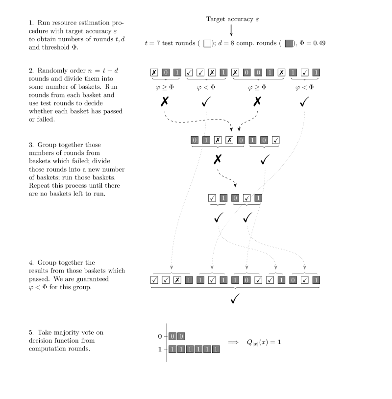
Figure 5: Contrived step-by-step example of our basketing technique for running an error mitigation protocol from the framework with some initial target accuracy $\varepsilon$. The first iteration uses four baskets whilst the second and third iterations use two baskets. For the first iteration, the first basket fails since the proportion of failed test rounds is $\varphi=0\geq\Phi=0.49$, the second passes since $\varphi=\frac{1}{3}<\Phi=0.49$ and so on. Once there are no more iterations left to run, those rounds from baskets which passed are grouped together and a majority vote is taken on the results from the computation rounds to give a final returned value of the decision function $Q_{|x|}(x)$.

Protocol 1.

Basketing protocol Client’s inputs: A $\mathsf{BQP}$ computation with corresponding MBQC pattern $\mathcal{P}$ as according to Section II.0.2. A definition of test rounds (e.g. Subroutine 2) and a corresponding resource estimation procedure (e.g. Subroutine 3). Protocol steps: 1. The Client uses the details of $\mathcal{P}$ to run the resource estimation procedure as discussed in Section III, obtaining values of the parameters $t,d\in\mathbb{N}$ and $\Phi\in(0,1)$. The Client sets $T=t$, $D=d$ and $N=T+D$. 2. The Client chooses a uniformly random partition $[N]=\mathbf{T}\cup\mathbf{D}$ where $|\mathbf{T}|=T$ and $|\mathbf{D}|=D$. Choose also $B\in\mathbb{N}$ and a uniformly random partition $[N]=\bigcup_{i\in[B]}B_{i}$ with $B_{i}\cap B_{j}=\emptyset\ \forall\ i\neq j$ and with $i<j\implies x<y\ \forall\ x\in B_{i},\ y\in B_{j}$ – i.e. the baskets contain disjoint batches of consecutive rounds. 3. For each basket $B_{i}$ with $i=1,2,\dots,B$: (a) For each round $r\in B_{i}$ (chosen in ascending order): • If $r\in\mathbf{D}$ (computation round), the Client runs Subroutine 1 on the Server and records the returned value of the decision function $Q_{|x|}(x)$. • If $r\in\mathbf{T}$ (test round), the Client runs their chosen test round subroutine on the Server and records whether the test round passes or fails. (b) Let $\varphi_{i}$ be the proportion of test rounds which failed across basket $i$; basket $i$ passes if $\varphi_{i}<\Phi$ and fails if $\varphi_{i}\geq\Phi$. 4. Let $\mathcal{F}\subseteq[B]$ be the set of indices from those baskets which failed. If $\mathcal{F}=\emptyset$, move on to Step 5. Else, define T = ∑_i ∈F — {r ∈B_i — r ∈T } —,  D = ∑_i ∈F — {r ∈B_i — r ∈D } —,  N = T + D and return to Step 2. 5. Upon reaching this step, $B$ baskets in total have now passed across all iterations; these $B$ baskets contain a total $t$ test rounds and $d$ computation rounds and there are no baskets left to run. The above process guarantees that the proportion $\varphi$ of test rounds which failed across these $B$ baskets is less than the threshold $\Phi$. Let the values of the decision function obtained from the $d$ computation rounds be $\{Q_{|x|}^{(i)}(x)\}_{i\in[d]}$; the Client computes $\mu=\sum_{i\in[d]}Q_{|x|}^{(i)}(x)$ and returns 0 if $\mu<\frac{d}{2}$, 1 if $\mu>\frac{d}{2}$ and Abort if $\mu=\frac{d}{2}$.

Figure 6: Statement of the basketing protocol in which $t$ test rounds and $d$ computation rounds are divided into $B$ ‘baskets’. Each basket separately samples the device noise and baskets deemed too noisy are discarded. For each iteration, we repeat those rounds from those discarded baskets from the previous iteration. For $n\in\mathbb{N}$ we define $[n]=\{1,2,\dots,n\}$.

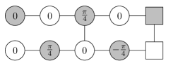
Figure 7: 10-qubit MBQC pattern for the controlled-$X$ gate. Numbers numbers indicates the measurement angles $\phi_{v}$ of the corresponding qubits to be used during computation rounds. The colour indicates the $k$-colouring ($k=2$) of the test rounds. The square vertices represent the two output qubits which are measured in the standard basis.

V Numerical examples

We illustrate the benefits of our work by running three comparative sets of classical simulations to compare both the original verification protocol and our error mitigation protocol using an MBQC simulator. We believe this work constitutes the first such classical simulations of the MBQC model for an error mitigation or verification purpose.

We provide a summary of our results here whilst a more detailed description of these numerical simulations is given in Appendix A.

We consider the theoretically straightforward example of implementing the computation

$$\ket{11}\mapsto\mathbf{CX}\ket{11}=\ket{10}$$

followed by a measurement of the two output qubits. This operation on two qubits can be encoded using the 10-qubit MBQC pattern given in Figure 7, which shows the measurement angles for the computation rounds and the colours for the test rounds. The underlying graph for this pattern is that of the brickwork state, introduced in [31], which when tiled is sufficient for universal quantum computation. Note that we have used the lowest possible value of $k=2$ for $k$-colouring our test rounds, corresponding to the discussion of Section III. The result of this computation is deterministic in a noiseless environment and hence the implicit $\mathsf{BQP}$ error rate is $p=0$.

Suppose the corresponding measurement outcome is $x$, then we define the decision function via

$$Q(x)=\begin{cases}0&\text{if }x\in\{00,01,11\};\\ 1&\text{if }x=10.\end{cases}$$ (16)

Our simulations are performed using a classical MBQC simulator with a fluctuating time-dependent noise model applied which is dictated by a single parameter $\Sigma$ which remains constant within each basket; details are given in Appendix A. Each basket consists of 10 rounds chosen consecutively according to the initial randomisation.

We now perform three comparative pairs of simulations, where in each case we wish to run the above computation with local-correctness upper bound $\varepsilon_{\text{max}}=0.01$. These simulations are designed to illustrate the following three cases in which we believe our error mitigation protocol to be advantageous over simply running the original verification protocol:

1. The verification protocol cannot be run whilst our error mitigation protocol can (‘high noise’);

2. The verification protocol requires an unfeasible number of device runs whilst our error mitigation procedure enables a feasible overhead (‘medium noise’);

3. Both protocols can feasibly be run, but our basketing protocol enables a substantial reduction in overhead (‘low noise’).

We discuss these cases in more detail in Appendix A.

V.0.1 High noise $(\Sigma=\pi/2)$

In the first simulation, we consider high-level fluctuating noise ($\Sigma=\pi/2$) and show that the verification protocol cannot be run whilst the basketing protocol is able to lift the correct signal from the noisy background. This hence gives evidence that our protocol is able to substantially alleviate the noise-sensitivity bottleneck of the verification work in an error mitigation context.

By simulating a large number (25,000) of test rounds under this noise model, we found a high empirical error rate of 62.3% and hence safely upper-bound this value with $p_{\text{max}}=0.7$. Running the minimisation of Section III subject to $\varepsilon_{\text{max}}=0.01$ and $p_{\text{max}}=0.7$, we were unable to produce convergence of the resource estimation procedure (since inequality 14 cannot be satisfied) and hence the standard verification protocol cannot be run.

Meanwhile, to run our basketing protocol we can remove the condition on $p_{\text{max}}$ and allow it to be chosen by the minimiser. Now, the resource estimation procedure successfully converges, returning $n=2190$ (to the nearest multiple of 10) with $t=1384,d=806,p_{\text{max}}=0.0100$, threshold $\Phi=0.1454$ and accuracy $\varepsilon=0.01000$. Running the basketing protocol with these parameters, we find that 628 of the 806 computation rounds ($77.9\%>50\%$) produce the correct classical outcome 10 (encoded as $Q=1$) and hence we obtain the correct result from the protocol. The resulting overhead is 1305 baskets, i.e. 13050 circuit runs.

Hence, our error mitigation protocol is able to be run in situations where the original verification protocol cannot be used.

V.0.2 Medium noise $(\Sigma=\pi/6)$

In our second simulation, we instead consider ‘medium’ fluctuations ($\Sigma=\pi/6$) and show that our basketing approach is able to dramatically reduce the required overhead of circuit runs versus the verification approach. Under this model, simulation of 25,000 test rounds gives a failure rate of 23.2% which we upper-bound with $p_{\text{max}}=0.24$.

To simulate the standard verification protocol, we run the resource estimation procedure with constraints $\varepsilon_{\text{max}}=0.01$ and $p_{\text{max}}=0.24$, obtaining $n\approx 50990000$. This evidently constitutes an overhead which is too large to be feasibly run.

Meanwhile, to simulate the basketing protocol we again remove the condition on $p_{\text{max}}$. In this case the minimisation returns $n=2060$ with $t=1001,\ d=1059,\ p_{\text{max}}=0.0100$, threshold $\Phi=0.1539$ and accuracy $\varepsilon=0.01000$. Running the basketing protocol with these parameters returns the correct result 10, with 951 of 1059 computation rounds (89.8%) returning this value and a total overhead of 505 baskets, i.e. 5050 circuit runs. Hence, we find that our basketing protocol has returned the correct result in a situation in which the standard verification protocol requires massive overhead.

V.0.3 Low noise $(\Sigma=\pi/12)$

Finally, we consider low level noise ($\Sigma=\pi/12$) in which both the verification and error mitigation protocols can feasibly be run, showing that in this case our approach is able to produce a substantial reduction in overhead. Under this model, simulation gives a test round failure rate of 9.3% which we upper bound with $p_{\text{max}}=0.1$.

For the standard verification protocol, our resource estimation procedure with $p_{\text{max}}=0.1$ returns an overhead of $n=10000$ device runs with $t=8817,d=1183$ and threshold $\Phi=0.1390$. Running the verification protocol returns the correct outcome 10 with a computation round success rate of 1117/1183 (94.4%) and a test round failure rate of 813/8817 (9.2%).

For the basketing protocol, we reduce $p_{\text{max}}=0.01$ and run the resource estimation procedure, obtaining $n=910$ with $t=709,d=201$ and threshold $\Phi=0.07845$. In this case, the basketing protocol also returns the correct outcome 10, requiring a total of 135 basket runs (1350 rounds) – substantially lower than in the verification case. The computation round data is also slightly higher quality with a success rate of 195/201 (97.0%).

VI Conclusions and future work

In this paper, we have introduced a scalable and noise-robust error mitigation protocol for computations from the $\mathsf{BQP}$ complexity class. This framework utilises trappification-based error-detection techniques from an existing quantum verification protocol where standard runs of the computation are interleaved with test rounds for error-detection. Our work hence inherits the property of being exponentially accurate with the total number of device runs. Moreover, the protocol requires no strict noise model or device tomography and hence is widely applicable to existing hardware, and able to scale to large numbers of qubits. We introduced the idea of basketing on top of the standard verification to address time-dependent noise behaviours using post-selection; we showed that this can be used to reduce the likelihood of the protocol aborting and to reduce the required overhead of circuit runs by running classical simulations in the measurement-based quantum computing framework under a fluctuating noise model.

Set within the measurement-based quantum computing framework, our protocol can be directly implemented on photonic platforms such as Quandela [38], QuiX Quantum [39], ORCA Computing [40] and PsiQuantum [41]. Moreover, we outlined a compilation strategy enabling our framework to be implemented on the wide array of device architectures which rely on the circuit model, provided they support adaptive mid-circuit measurements.

Throughout this paper, we have intentionally used a modular approach such that the subroutines for test rounds, computation rounds and resource estimation are separated. One particular reason for this approach was to enable the potential for other test rounds to be integrated. For example, the recent verification work of [25] proposes ‘dummyless’ test rounds which effectively remove the factor of $\frac{1}{k}$ in the upper-bound of the threshold $\Phi$ in Theorem 1. It is at present, however, much harder to define a clear algorithmic resource estimation procedure using these tests, and hence we leave their implementation to future work. We also anticipate that further work will be able to address the case in which the Client suffers from state-preparation noise, and will be able to consider more general classes of computation. Furthermore, we anticipate the potential to develop test rounds which are suited to specific applications or device architectures. Hence, future work on the topic may be to propose a framework for a class of trappification-based error mitigation protocols with differing test rounds designs.

On the simulation side, we recognise the limitations of the noise model which we used in Section V as a result of the limitations of the simulator. We hope to perform further informative simulations using a simulator on which much more general noise maps can be applied. Similarly, we would like demonstrate our protocol in the circuit model on a device which supports mid-circuit adaptive measurements.

Efficient compilation strategies transforming generic circuit model computations to the formatting of Section III would be highly beneficial for the implementation of this protocol within the circuit model. This would especially be the case if one were able to reduce the dependence on mid-circuit adaptive measurements.

Finally, the numerical results shown in Figures 8 and 9 show substantial differences between the value of $n$ and the overhead of circuit runs when running our basketing protocol. An improved resource estimation procedure should be able to take into account basket repetitions in order to estimate the total number of device runs that may be required to run the basketing protocol, in particular identifying situations in which this overhead might be substantial due to large numbers of baskets being repeated. Despite these repetitions, however, the simulations of Section V.0.2 showed that we were able to dramatically reduce the required overhead versus running the standard verification protocol of [20].

VII Acknowledgements

Both authors acknowledge funding from Innovate UK as part of the national Auto-Calibration project. We also thank Dominik Leichtle and Harold Ollivier their contributions in explaining the applicability of the underlying verification work of [20] and [25].

Appendix

Method	$\Sigma$	$p_{\text{max}}$	$n$	$\tau$	$\psi$	$\varepsilon_{1}$	$\varepsilon_{2}$	$\varepsilon_{3}$	$\Phi$
Verification	$\pi/2$	0.7	Minimisation did not converge
Basketing	$\pi/2$	0.01	2190	0.6321	0.1055	0.04679	0.08185	0.06099	0.1454
Verification	$\pi/6$	0.24	50990000	0.4721	0.004861	0.001010	0.01363	0.004636	0.2403
Basketing	$\pi/6$	0.01	2060	0.4857	0.08199	0.04801	0.08407	0.04364	0.1539
Verification	$\pi/12$	0.1	10000	0.8817	0.1920	0.01231	0.02988	0.1597	0.1390
Basketing	$\pi/12$	0.01	910	0.7783	0.2452	0.04272	0.1301	0.1623	0.07845

Figure 8: Table stating the minimisation parameters obtained for each simulation with values to four significant figures. Each minimisation also used $p=0$ and returned $\varepsilon=0.01000$ to four significant figures. In the verification cases, the value of $p_{\text{max}}$ was fixed as described below.

Method	$\Sigma$	Overhead (circuit runs)	Comp. success rate	Test failure rate	Output
Verification	$\pi/2$	Minimisation did not converge			Abort
Basketing	$\pi/2$	13050	77.9%	–	Accept $Q=1$
Verification	$\pi/6$	50990000	Required overhead too high to run		Abort
Basketing	$\pi/6$	5050	89.8%	–	Accept $Q=1$
Verification	$\pi/12$	10000	94.4%	9.2%	Accept $Q=1$
Basketing	$\pi/12$	1350	97.0%	–	Accept $Q=1$

Figure 9: Table comparing the results for each classical simulation. $Q$ is defined in equation 16 such that an output $Q=1$ corresponds to successful detection of the classical output 10. Each simulation that run has a local-correctness bound $\varepsilon_{\text{max}}=0.01$.

Appendix A Details of numerical simulation

In this section, we provide a more detailed description of the numerical simulations used in Section V.

A.0.1 Simulating noisy MBQC

We produced a classical noisy simulation of the measurement-based quantum computation (MBQC) framework of Section II.0.2 using the Paddle Quantum simulator [42]. Note that the actions of a quantum device in MBQC can be reduced to two kinds:

• State preparation: the device prepares a qubit in the state $\ket{+_{\theta}}=\frac{1}{\sqrt{2}}(\ket{0}+e^{i\theta}\ket{1})$, where $\theta\in\Theta$, and applies CZ gates between pairs of qubits to produce the graph state;

• Measurement: the device measures a qubit according to the basis $M_{XY}(\theta)=\{\ket{+_{\theta}},\ket{-_{\theta}}\}$, where $\theta\in\Theta$,

with $\Theta=\{\frac{k\pi}{4}\}_{k=0}^{7}$. The device also applies Pauli $X$ and $Z$ corrections to the output qubits, but we assume to be considering patterns large enough that noise from this stage can be neglected. Hence, as a natural way of simulating noise under the limitations of the simulator, we considered the case of applying normally distributed perturbations to the state preparation and measurement angles:

• Noisy state preparation: the device prepares a qubit in the state $\ket{+_{\theta+\delta\theta}}$ where $\theta\in\Theta$ and $\delta\theta\sim N(0,\sigma^{2})$;

• Noisy measurement: the device measures a qubit according to the basis $M_{XY}(\theta+\delta\theta)$ where $\theta\in\Theta$ and $\delta\theta\sim N(0,\sigma^{2})$,

for some $\sigma$ quantifying the noise level in either case. For simplicity in our simulations we set the noise level to be equal for both kinds of noise. We acknowledge that a better model would involve the inclusion of more general noise maps such as depolarising channels, but the application of quantum channels mid-way through the execution of an MBQC pattern is not supported by the simulator.

In our noise model, we consider the case of fluctuating time-dependent noise $\sigma\in\text{Uniform}(0,\Sigma)$ for a fixed $\Sigma$ dictating the overall noise strength. Each noise level $\sigma$ lasts for 50 consecutive device runs before another value is chosen randomly and independently according to the above distribution. Each basket consists of 10 rounds such that the noise level $\Sigma$ is constant within each basket. Baskets containing no test rounds are automatically rejected.

A.0.2 Choice of simulations

Our objective is to show that, in the context of running a $\mathsf{BQP}$ computation on a trusted device with time-dependent fluctuating noise to some required accuracy $\varepsilon$, our basketing protocol is both successful and preferable to the existing verification protocol of Section II.0.3.

We believe there are three possible cases worth consideration.

The first is the case in which our average device noise (and hence $p_{\text{max}}$) is so high that the minimisation of Section III cannot converge. Post-selection allows us to force $p_{\text{max}}$ to be low enough that the minimisation does converge, leading to situations in which our basketing protocol can be run whilst the original verification protocol cannot. For this case we set $\Sigma=\pi/2$.

The second is the case of medium-strength noise whereby the minimisation can converge but does not produce feasible parameters in the verification case, whilst it does in the error mitigation case, where $p_{\text{max}}$ is unrestricted. For this case we set $\Sigma=\pi/6$.

The final case is that of low-strength noise in which both protocols can feasibly be run. Reducing the value of $p_{\text{max}}$ in this case allows us to reduce the initial total number of rounds $n$ and hence the total overhead of circuit runs. We also show in this case that the data returned by the basketing protocol is of typically higher quality. For this case we set $\Sigma=\pi/12$.

The reason for the existence of these distinct cases can be seen in Lemma 4 of [20]. In summary, if $p_{\text{max}}\geq\frac{1}{2}$ then the minimisation will necessarily not converge. If $p_{\text{max}}<\frac{1}{2}$ then there are two distinct regimes depending on the value of $\Phi$ – one in which failure is overwhelmingly likely without an exponential overhead, and the other (that of Theorem 1) in which we get exponentially-scaling local correctness.

A.0.3 Choice of computation

We would like to consider a computation which is theoretically straightforward in terms of the applied unitary whilst allowing us to consider noise across a relatively large (at the scale of classical simulability) number of qubits. Hence, we opt to use the 10-qubit pattern which implements the 2-qubit controlled-$X$ (CX) gate as shown in Figure 7. Specifically, we consider the pattern with quantum input $\ket{11}$ (i.e. $x=11$), such that a computational basis measurement of the two output qubits should return $10$; hence we define the decision function of this computation via

$$Q(x)=\begin{cases}0&\text{if }x\in\{00,01,11\};\\ 1&\text{if }x=10.\end{cases}$$ (17)

The result of this computation is deterministic in a noiseless environment and hence the implicit $\mathsf{BQP}$ error rate is $p=0$. Figure 7 also shows the $k=2$ $k$-colouring used for the design of the test rounds.

A.0.4 Calculating global parameters

We consider the calculation of global parameters which will take the same value across all simulations. Recall that, returning to the notation of Section III, the variables $p,k$ and $p_{\text{max}}$ (in the verification case) are chosen using knowledge of our target $\mathsf{BQP}$ computation and our (simulated) noisy quantum device.

Since the computation will deterministically produce the correct result in the absence of noise, the implicit $\mathsf{BQP}$ error rate is $p=0$ across all simulations.

Finally, the value of $p_{\text{max}}$, an upper-bound on the error rate of the test rounds under our noise models, is calculated empirically. Specifically, we run 25,000 test rounds under each of the three noise levels and calculate the proportions which fail. For the high, medium and low noise cases, these proportions were 0.623, 0.232 and 0.093 respectively and hence we set $p_{\text{max}}=0.7,0.24,0.1$ for these three cases.

A.0.5 Running minimisation

Our parameter values are calculated according to the minimisation technique described in Section III. The algorithm for this minimisation is implemented in Python using the scipy.optimize.minimize library [43] with the Sequential Least Squares Programming method.

Across all minimisations, the algorithm’s objective is to minimise the value of $n$ subject the condition $\varepsilon_{\text{max}}=0.01$, as well as conditions 3 to 14. In each case the minimisation returns $\varepsilon=0.01000$ to four significant figures. For the verification protocol, we also condition that $p_{\text{max}}$ takes the specific values detailed above. For the basketing protocol, we only condition that $p_{\text{max}}\geq 0.01$ – this prevents the algorithm from unintentionally converging to the non-useful case in which $p_{\text{max}}\approx\Phi\approx 0$. We note, however, that the minimisation typically prefers to minimise the value of $p_{\text{max}}$ and hence the minimiser tends to set $p_{\text{max}}$ to be equal to this lower bound.

A breakdown of the obtained parameter values for each cases is given in Figure 8.

A.0.6 Running simulations

Our simulations were performed using our noisy MBQC simulator described above. We constructed these simulations such that they return more data than returned than is required by the protocols, e.g. if the verification protocol returns Abort, it also returns the proportion of test rounds that failed. Of interest to us was the proportion of failed test rounds (for the verification protocol only), the proportion of correct computation rounds (for both protocols) and the total overhead of circuit runs (for the basketing protocol only).

These results for all four simulations are shown in Figure 9.

References

- Strikis et al. [2021] A. Strikis, D. Qin, Y. Chen, S. C. Benjamin, and Y. Li, Learning-based quantum error mitigation, PRX Quantum 2, 040330 (2021).
- Suzuki et al. [2022] Y. Suzuki, S. Endo, K. Fujii, and Y. Tokunaga, Quantum error mitigation as a universal error reduction technique: Applications from the nisq to the fault-tolerant quantum computing eras, PRX Quantum 3, 010345 (2022).
- Endo et al. [2018] S. Endo, S. C. Benjamin, and Y. Li, Practical quantum error mitigation for near-future applications, Physical Review X 8, 031027 (2018).
- Endo et al. [2021a] S. Endo, Z. Cai, S. C. Benjamin, and X. Yuan, Hybrid quantum-classical algorithms and quantum error mitigation, Journal of the Physical Society of Japan 90, 032001 (2021a).
- Takagi et al. [2022] R. Takagi, S. Endo, S. Minagawa, and M. Gu, Fundamental limits of quantum error mitigation, npj Quantum Information 8, 114 (2022).
- Li and Benjamin [2017] Y. Li and S. C. Benjamin, Efficient Variational Quantum Simulator Incorporating Active Error Minimization, Physical Review X 7, 021050 (2017), 1611.09301 .
- Temme et al. [2017] K. Temme, S. Bravyi, and J. M. Gambetta, Error Mitigation for Short-Depth Quantum Circuits, Physical Review Letters 119, 180509 (2017), 1612.02058 .
- Giurgica-Tiron et al. [2020] T. Giurgica-Tiron, Y. Hindy, R. LaRose, A. Mari, and W. J. Zeng, Digital zero noise extrapolation for quantum error mitigation, in 2020 IEEE International Conference on Quantum Computing and Engineering (QCE) (2020) pp. 306–316.
- He et al. [2020] A. He, B. Nachman, W. A. de Jong, and C. W. Bauer, Zero-noise extrapolation for quantum-gate error mitigation with identity insertions, Phys. Rev. A 102, 012426 (2020).
- Song et al. [2019] C. Song, J. Cui, H. Wang, J. Hao, H. Feng, and Y. Li, Quantum computation with universal error mitigation on a superconducting quantum processor, Science Advances 5, eaaw5686 (2019), https://www.science.org/doi/pdf/10.1126/sciadv.aaw5686 .
- Mari et al. [2021] A. Mari, N. Shammah, and W. J. Zeng, Extending quantum probabilistic error cancellation by noise scaling, Phys. Rev. A 104, 052607 (2021).
- van den Berg et al. [2022] E. van den Berg, Z. K. Minev, A. Kandala, and K. Temme, Probabilistic error cancellation with sparse pauli-lindblad models on noisy quantum processors (2022), arXiv:2201.09866 [quant-ph] .
- Koczor [2021] B. Koczor, Exponential error suppression for near-term quantum devices, Phys. Rev. X 11, 031057 (2021).
- Huggins et al. [2021] W. J. Huggins, S. McArdle, T. E. O’Brien, J. Lee, N. C. Rubin, S. Boixo, K. B. Whaley, R. Babbush, and J. R. McClean, Virtual distillation for quantum error mitigation, Phys. Rev. X 11, 041036 (2021).
- Teo et al. [2023] Y. S. Teo, S. Shin, H. Kwon, S.-H. Lee, and H. Jeong, Virtual distillation with noise dilution, Phys. Rev. A 107, 022608 (2023).
- Vikstål et al. [2022] P. Vikstål, G. Ferrini, and S. Puri, Study of noise in virtual distillation circuits for quantum error mitigation (2022), arXiv:2210.15317 [quant-ph] .
- Huo and Li [2022] M. Huo and Y. Li, Dual-state purification for practical quantum error mitigation, Phys. Rev. A 105, 022427 (2022).
- Quek et al. [2023] Y. Quek, D. S. França, S. Khatri, J. J. Meyer, and J. Eisert, Exponentially tighter bounds on limitations of quantum error mitigation (2023), arXiv:2210.11505 [quant-ph] .
- Endo et al. [2021b] S. Endo, Z. Cai, S. C. Benjamin, and X. Yuan, Hybrid Quantum-Classical Algorithms and Quantum Error Mitigation, Journal of the Physical Society of Japan 90, 032001 (2021b), 2011.01382 .
- Leichtle et al. [2021] D. Leichtle, L. Music, E. Kashefi, and H. Ollivier, Verifying bqp computations on noisy devices with minimal overhead, PRX Quantum 2, 040302 (2021).
- Mezher et al. [2022] R. Mezher, J. Mills, and E. Kashefi, Mitigating errors by quantum verification and postselection, Physical Review A 105, 052608 (2022), 2109.14329 .
- Nielsen and Chuang [2010] M. A. Nielsen and I. L. Chuang, Quantum Computation and Quantum Information: 10th Anniversary Edition (Cambridge University Press, 2010).
- Raussendorf et al. [2003] R. Raussendorf, D. E. Browne, and H. J. Briegel, Measurement-based quantum computation on cluster states, Physical Review A 68, 022312 (2003), quant-ph/0301052 .
- Danos and Kashefi [2006] V. Danos and E. Kashefi, Determinism in the one-way model, Phys. Rev. A 74, 052310 (2006).
- Kapourniotis et al. [2022] T. Kapourniotis, E. Kashefi, D. Leichtle, L. Music, and H. Ollivier, Unifying quantum verification and error-detection: Theory and tools for optimisations (2022), arXiv:2206.00631 [quant-ph] .
- Gheorghiu et al. [2018] A. Gheorghiu, T. Kapourniotis, and E. Kashefi, Verification of quantum computation: An overview of existing approaches, Theory of Computing Systems 63, 715 (2018).
- Barz et al. [2013] S. Barz, J. F. Fitzsimons, E. Kashefi, and P. Walther, Experimental verification of quantum computation, Nature Physics 9, 727 (2013).
- Mahadev [2018] U. Mahadev, Classical verification of quantum computations, in 2018 IEEE 59th Annual Symposium on Foundations of Computer Science (FOCS) (2018) pp. 259–267.
- Carrasco et al. [2021] J. Carrasco, A. Elben, C. Kokail, B. Kraus, and P. Zoller, Theoretical and experimental perspectives of quantum verification, PRX Quantum 2, 010102 (2021).
- Mavadia et al. [2018] S. Mavadia, C. L. Edmunds, C. Hempel, H. Ball, F. Roy, T. M. Stace, and M. J. Biercuk, Experimental quantum verification in the presence of temporally correlated noise, npj Quantum Information 4, 10.1038/s41534-017-0052-0 (2018).
- Broadbent et al. [2010] A. Broadbent, J. Fitzsimons, and E. Kashefi, Measurement-Based and Universal Blind Quantum Computation, Formal Methods for Quantitative Aspects of Programming Languages, 10th International School on Formal Methods for the Design of Computer, Communication and Software Systems, SFM 2010, Bertinoro, Italy, June 21-26, 2010, Advanced Lectures , 43 (2010).
- Maurer and Renner [2011] U. Maurer and R. Renner, Abstract cryptography, in The Second Symposium on Innovations in Computer Science, ICS 2011, edited by B. Chazelle (Tsinghua University Press, 2011) pp. 1–21.
- Harper and Flammia [2017] R. Harper and S. T. Flammia, Estimating the fidelity of t gates using standard interleaved randomized benchmarking, Quantum Science and Technology 2, 015008 (2017).
- Cai and Benjamin [2019] Z. Cai and S. C. Benjamin, Constructing smaller pauli twirling sets for arbitrary error channels, Scientific Reports 9, 10.1038/s41598-019-46722-7 (2019).
- Morvan et al. [2021] A. Morvan, V. V. Ramasesh, M. S. Blok, J. M. Kreikebaum, K. O’Brien, L. Chen, B. K. Mitchell, R. K. Naik, D. I. Santiago, and I. Siddiqi, Qutrit randomized benchmarking, Phys. Rev. Lett. 126, 210504 (2021).
- Brown and Eastin [2018] W. G. Brown and B. Eastin, Randomized benchmarking with restricted gate sets, Phys. Rev. A 97, 062323 (2018).
- Boone et al. [2019] K. Boone, A. Carignan-Dugas, J. J. Wallman, and J. Emerson, Randomized benchmarking under different gate sets, Phys. Rev. A 99, 032329 (2019).
-
[38]
Quandela - Photonic
Quantum Computers, https://www.quandela.com/,
(accessed 6 June 2023). -
[39]
QuiX Quantum -
Home, https://www.quixquantum.com/,
(accessed 6 June 2023). -
[40]
Photonic quantum
computers for Machine Learning, https://www.orcacomputing.com/,
(accessed 6 June 2023). -
[41]
PsiQuantum —
Photonic Quantum Computing, https://psiquantum.com/about,
(accessed 6 June 2023). - Pad [2023] Paddle Quantum – MBQC Quick Start Guide, https://qml.baidu.com/tutorials/measurement-based-quantum-computation/mbqc-quick-start-guide.html ((accessed 6 June 2023)).
- [43] scipy.optimize.minimize — SciPy v1.10.0 Manual, (accessed 6 June 2023).