Towards a Benchmark for Markov State Models:
The Folding of HP35

Abstract

Adopting a $300\,\upmu$s-long molecular dynamics (MD) trajectory of the reversible folding of villin headpiece (HP35) published by D. E. Shaw Research, we recently constructed a Markov state model (MSM) of the folding process based on interresidue contacts [J. Chem. Theory Comput. 2023, 19, 3391]. The model reproduces the MD folding times of the system and predicts that both the native basin and the unfolded region of the free energy landscape are partitioned into several metastable substates that are structurally well characterized. Recognizing the need to establish well-defined but nontrivial benchmark problems, in this Perspective we study to what extent and in what sense this MSM may be employed as a reference model. To this end, we test the robustness of the MSM by comparing it to models that use alternative combinations of features, dimensionality reduction methods and clustering schemes. The study suggests some main characteristics of the folding of HP35, which should be reproduced by any other competitive model of the system. Moreover, the discussion reveals which parts of the MSM workflow matter most for the considered problem, and illustrates the promises and possible pitfalls of state-based models for the interpretation of biomolecular simulations.

1 Introduction

Molecular dynamics (MD) simulations allow us to study the structure, dynamics and function of biomolecular systems in atomic detail.¹ To facilitate a concise interpretation of the resulting ’big data’, it is common practice to construct a coarse-grained model of the considered process, e.g., based on a Langevin equation^{2, 3, 4} or a Markov state model (MSM). ^{5, 6, 7, 8, 9, 10, 11, 12} Interpreting MD trajectories in terms of memoryless transitions between metastable conformational states, MSMs have become particularly popular as they provide a generally accepted state-of-the-art analysis of the dynamics,^{9, 10, 11} promise to predict long-time dynamics from short trajectories,^{13, 14} and are straightforward to build using open-source packages such as PyEmma ¹⁵ and MSMBuilder.¹⁶ The generally accepted workflow to construct an MSM consists of five steps: (1) featurization, i.e., selection of suitable input coordinates, (2) dimensionality reduction from the high-dimensional feature space to a low-dimensional space of collective variables, (3) geometrical clustering of these low-dimensional data into microstates, (4) dynamical clustering of the microstates into metastable conformational states, and (5) estimation of the corresponding transition matrix.

In recent years, the groups of Noé and Pande and several others have established a comprehensive mathematical formulation of Markov modeling.^{8, 9, 10, 11, 12} This includes their derivation from exact generalized master equations¹⁷ and transition operator theory,¹⁸ their application to nonequilibrium processes, ^{19, 20, 21} their combination with multiensemble ²² and adaptive sampling methods, ¹⁴ and their extension to approaches including memory such as core-set MSMs ^{7, 23, 24, 25} and memory-enriched models. ^{26, 21, 27, 28} In particular, it has been shown that the quality of an MSM can be optimized by employing a variational principle,^{29, 30} which states that the MSM producing the slowest implied timescales represents the best approximation to the true dynamics. As a consequence, the resulting MSM is dynamically consistent, that is, it reproduces the correct coarse-grained dynamics, as can be checked by comparison to reference MD data. While the variational approach in principle provides a rigorous means to construct MSMs, its meaningful application to all five steps of the workflow rests on several assumptions. For example, the considered process needs to be sufficiently sampled (to ensure that the MD data are statistically significant) as well as appropriately described by the chosen input coordinates (to enable a successful model from the outset).

What is more, we want to assure that the resulting MSM meets its original purpose, i.e., to explain the mechanism of a biomolecular process in terms of transitions between functionally relevant and structurally well-characterized metastable states. MSMs represent a spatio-temporal coarse graining of the MD simulation, where the lag time $\tau_{\rm lag}$ (for which the transition matrix is calculated) defines the time resolution and the conformational ensembles represented by the states define the spatial resolution. Hence, $\tau_{\rm lag}$ needs to be shorter than the fastest dynamics of interest, and the spatial resolution provided by the state partitioning needs to be sufficient to account for the relevant microscopic steps of the functional motion. Unfortunately, these requests are often in conflict with the requirement of slow implied timescales enforced by variational methods. For example, while shorter lag times improve the time resolution, they have the undesirable effect of shortening the timescales of the MSM, hence resulting in the loss of Markovianity. Nevertheless, so far most existing strategies to optimize MSMs (e.g., via the selection of its hyperparameters) are solely based on the variational approach.^{31, 32} Hence there is a demand to establish well-defined criteria that ensure that an MSM also provides the desired microscopic interpretation. Recently proposed extensions of MSMs including memory may be a resort in this respect, ^{26, 21, 27, 33, 28} since they hold the promise to construct dynamic models with a sufficiently high spatio-temporal resolution to account in detail for the mechanisms, while still providing a dynamically consistent description including the correct long timescales.

At present, the development of post-simulation models such as Langevin equations and MSMs is at a transition point from gathering concepts and ideas to a systematic, consistent, and well-understood methodology. Similar as in more mature research fields such as electron structure theory and force field development, this requires an agreement of the community on well-defined benchmark problems, key observables of interest, and clear criteria of quality assessment.³⁴ This is particularly important, for example, when we want to assess the rapidly increasing number of machine-learning empowered methods of conformational analysis (see Refs. 35, 36, 37, 38 for recent reviews). So far mostly the “alanine dipeptide” (sequence Ace-Ala-Nme) has served as a benchmark problem, because the system is well represented by two backbone dihedral angles $(\phi,\psi)$ and thus quite simple to model.^{39, 40, 41} Moreover various short peptides that form metastable secondary structures have been considered.

To move towards more biophysically relevant systems, the obvious next step is to establish a benchmark model of a simple globular protein with a tertiary structure. As a prime example, here we consider the folding of the 35-residue villin headpiece, aka HP35, consisting of a hydrophobic core with three helices that are connected via two short loops (Fig. 1a). Specifically, we adopt a $300\,\upmu$s-long trajectory at 360 K of the fast folding variant Lys24-Nle/Lys29-Nle, which is publicly available from D. E. Shaw Research.⁴² Showing 33 folding and 32 unfolding events (Fig. 1c), the simulation reproduces at least qualitatively some of the main experimental findings for the system,^{43, 44, 45, 46} including the melting temperature (370 K in MD vs. 361 K in experiment), the folding enthalpy (21 vs. 25 kcal/mol), as well as the folding time (1.8 vs. 0.7 $\mu$s). Being one of the smallest naturally occurring proteins that folds autonomously into a globular structure at record speed,^{45, 46} HP35 is probably the most intensively studied ultrafast folder by experiment, ^{44, 45, 46, 47, 48, 49, 50, 51, 52} MD simulation, ^{53, 54, 55, 56, 57, 58, 59, 42} and conformational analysis, ^{60, 61, 62, 24, 63, 64, 65, 66} and was featured as ’the new benchmark system of protein folding’ by Bill Eaton.⁵²

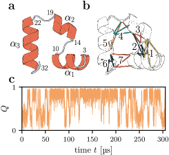
Figure 1: The folding of villin headpiece (HP35). (a) Molecular structure of the native state, consisting of three $\alpha$-helices (residues 3–10, 14–19 and 22–32) connected by two loops. (b) Illustration of the seven main clusters of native contacts, obtained from a MoSAIC correlation analysis⁶⁷ of the contact distances. (c) Time evolution of the fraction of native contacts $Q$ obtained from the folding trajectory by Piana et al.,⁴² showing reversible transitions between the unfolded region of the free energy landscape ($Q\lesssim 0.4$) and the native basin ($Q\gtrsim 0.7$).

While a large number of theoretical analyses have been performed on the long folding MD trajectories of D. E. Shaw Research, the resulting models are often hard to compare and their quality is difficult to assess. To a large extent this is caused by the very first step of the workflow, the choice of input coordinates or features. Since ’you get what you put in’, feature selection is crucial for every conformational analysis. ^{32, 64, 68, 69} Adopting the above mentioned trajectory of HP35 by Piana et al.,⁴² we recently performed a careful study of the effects of feature selection on Markov modeling.⁷⁰ As a main result, we showed that backbone dihedral angles account accurately for the structure of the native energy basin of HP35, while the unfolded region of the free energy landscape and the folding process are best described by tertiary contacts of the protein. In particular, we showed that the contact-based MSM describes consistently the hierarchical structure of the free energy landscape, that is, predicts that both the native basin and the unfolded region are structured into several metastable substates, evidence of which was shown in various experiments.^{46, 47, 48, 49, 50, 51, 52}

In this perspective, we wish to investigate to what extent and in what sense the contact-based MSM of Ref. 70 might be established as a reference or benchmark model of the coarse-grained folding dynamics of HP35. For one, the model satisfies our above discussed criteria, that is, provides structurally well-characterized metastable states that account for the folding pathways of HP35 (thus explaining the underlying mechanism) and whose dynamics compare well to reference calculations obtained from the MD trajectory (proving the dynamical consistence of the model). However, it is (most likely) not the best possible model and certainly not unique, because the MSM workflow necessitates the choice of numerous methods and metaparameters. As a minimum requirement for a reference model, we therefore evaluate the model’s robustness with respect to such variations by employing alternative methods for all steps of the MSM workflow. While it is neither possible nor desirable to exhaustively sample the high-dimensional ’method space’, the MSMs resulting from a few popular method combinations nevertheless give a qualitative idea of the accuracy and the quality that can be achieved by this type of modeling. In this way, we establish some main characteristics that we believe are intrinsic to the folding of HP35 (or at least to this specific trajectory), and therefore should be reproduced by any other competitive model of the system.

2 Results

2.1 Reference model

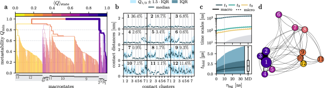
Figure 2: Contact-based model of HP35, using principal component analysis (PCA), robust density-based clustering (RDC) and the most probable path algorithm (MPP). (a) MPP dendrogram illustrating the clustering of microstates into metastable states upon increasing the requested minimum metastability criterion $Q_{\text{min}}$ of a state. (b) Structural characterization of the twelve metastable states of HP35. The states are ordered by decreasing fraction of native contacts $Q$, the contacts are ordered according to the seven main clusters (Fig. 1b). (c) First three implied timescales $t_{n}$ shown as a function of the lag time $\tau_{\text{lag}}$ and box-plot representation of the folding time distributions obtained from MSM and MD data. (d) Kinetic network of the MSM generated from the force-directed algorithm ForceAtlas2.⁷¹ The node size indicates the population of the state and the color code reflects its fraction of native contacts $Q$.

To define the contact-based MSM of HP35, we briefly introduce the methods used in the MSM workflow (for further details see Ref. 70). We begin with the choice of features, where we focused on native interresidue contacts, which are believed to largely determine the folding pathways of a protein, ^{72, 73, 74} as they account for the mechanistic origin of the studied process. Moreover, the fraction of native contacts represents a well-established one-dimensional reaction coordinate,^{74, 75} which nicely illustrates the overall time evolution of the folding (Fig. 1c). Here we assume a contact to be formed if the distance $d_{ij}$ between the closest non-hydrogen atoms of residues $i$ and $j$ is shorter than $4.5\text{\,}\mathrm{\text{\r{A}}}$, where $d_{ij}$ is the minimal distance between all atoms pairs of the two residues.^{70, 76} To focus on native contacts, we request that contacts between these atoms pairs are populated more than $30\text{\,}\%$ of the simulation time, which excludes nonnative contacts that are typically infrequent and short-lived.⁷⁰ To characterize the resulting 42 native contacts of HP35, we calculate the linear correlation matrix $\rho$ of their distances, and block-diagonalize $\rho$ using the Python package MoSAIC⁶⁷ (see Methods). This results in seven main clusters of highly correlated contacts, which change in a cooperative manner during the folding process. As the contacts of the clusters follow nicely the protein backbone from the N- to the C-terminus (Fig. 1b), the clusters can be employed to characterize the structure of the conformational states of the protein (see Fig. 2 below).

To construct metastable conformational states from the above defined trajectory of contact distances, the following protocol is used. In a first step, we eliminate high-frequency fluctuations of the distance trajectory, by employing a Gaussian low-pass filter with a standard deviation of $\sigma=2\,$ns. Aiming to avoid the misclassification of the data points in the transition regions, this simple procedure (prior to clustering) was found to perform better than using dynamic core sets ^{24, 65} following clustering. For dimensionality reduction we use principal component analysis (PCA) on the smoothed contact distances. ⁶³ The first five components exhibit a multimodal structure of their free energy curves, reveal the slowest timescales ($\sim 0.1$ to $2\text{\,}\mathrm{\SIUnitSymbolMicro s}$), and explain $\sim$80\text{\,}\%$$ of the total correlation. Using these collective variables, we next perform robust density-based clustering⁷⁷ (RDC), which computes a local free energy estimate for every frame of the trajectory by counting all other structures inside a hypersphere of fixed radius. By reordering all structures from low to high free energy, RDC directly yields the minima of the free energy landscape. Requesting a minimal population ($P_{\text{min}}=$0.01\text{\,}\%$\,\widehat{=}\,$153\text{\,}\mathrm{f}\mathrm{r}\mathrm{a}\mathrm{m}\mathrm{e}\mathrm{s}$$) each state must contain, we obtain 547 microstates.

In the next step, we adopt the most probable path algorithm⁷⁸ (MPP) to construct a small number of macrostates. Starting with the above defined microstates, MPP first calculates the transition matrix of these states, using a lag time $\tau_{\text{MPP}}=$10\text{\,}\mathrm{ns}$$. If the self-transition probability of a given state is lower than a certain metastability criterion $Q_{\text{min}}\in(0,1]$, the state will be lumped with the state to which the transition probability is the highest. Repeating the procedure for increasing $Q_{\text{min}}$, we construct a dendrogram that reveals how the various metastable states merge into energy basins, see Fig. 2a. For $Q_{\text{min}}\gtrsim 0.9$, we obtain only two macrostates, as all microstates are assigned to either the native or the unfolded energy basin of HP35. Coloring the states according to their mean number of native contacts, the native states are drawn in purple and the unfolded in yellow to orange. By decreasing the requested metastability $Q_{\text{min}}$, we in effect decrease the requested minimum barrier height between separated states, such that the two main basins split up in an increasing number of substates. To resolve at least the first tier of the emerging hierarchical structure, we require that the states should have at least $Q_{\text{min}}=0.5$ and a minimum population of $0.5\text{\,}\%$, thus obtaining 12 metastable states.⁷⁹ Remarkably, we find that the native basin as well as the unfolded basin splits up in various well-characterized states of high metastability.

As stressed in the Introduction, the metastable states of an MSM should represent distinct conformational ensembles, in order to allow for a detailed characterization of the folding mechanism. To provide such a structural characterization, Fig. 2b shows the distribution of contact distances for each state. The states are ordered by decreasing fraction of native contacts, such that state 1 is the native state (all contact distances are shorter than $4.5\text{\,}\mathrm{\text{\r{A}}}$) and state 12 is the completely unfolded state with a broad distribution of large distances. The contacts are ordered according to the seven main MoSAIC clusters shown in Fig. 1b, which follow the protein backbone from the N- to the C-terminus. The first three states are structurally well-defined native-like states that differ in details of helix 1 and contain $62\text{\,}\%$ of the total population. From the MPP dendrogram we learn that states 4 and 5 also belong to the native energy basin, and differ from state 1 by broken contacts on the C-terminal side. The unfolded basin consists of states 9 to 12, which show increasing degree of disorder. Furthermore, there are three lowly populated ($\lesssim$1\text{\,}\%$$) intermediate states. We note in passing that it is difficult to discriminate the metastable states via a visual inspection of their three-dimensional structural ensembles. This is because the main three native states exhibit only small structural differences, and because the structural ensembles of the unfolded states show a large variance. On the other hand, the contact representations in Fig. 2b provide a concise structural description of the states, because they directly account for the most important structural determinants of the folding process.

To assess the dynamical properties of the states, we calculate the transition matrix describing the probability of a transition between any two states during some chosen lag time $\tau_{\text{lag}}$. By diagonalizing this matrix, we obtain its eigenvalues $\lambda_{n}$ and the implied timescales $t_{n}=-\tau_{\text{lag}}/\ln{\lambda_{n}}$. To optimally project the microstate dynamics onto the macrostate dynamics, we use for the calculation of the transition matrix the method of Hummer and Szabo,⁸⁰ which ensures that the macrostate timescales closely approximate the microstate timescales. Figure 2c shows the resulting first three micro- and macrostate timescales $t_{1}$–$t_{3}$, which both are found to level off for lag times $\tau_{\text{lag}}\gtrsim$10\text{\,}\mathrm{ns}$$. For further reference, we summarize the quality of the implied timescales by a single number, the generalized matrix Rayleigh quotient (GMRQ),³¹ given by the sum of the first $3$ eigenvalues $\lambda_{n}$. For $\tau_{\text{lag}}=$10\text{\,}\mathrm{ns}$$, we obtain GMRQ$=2.80$. (Note that its theoretical maximum value is 3.) To see how the implied timescales translate to measurable observables of the folding process, we also consider the distribution of the folding time $t_{\text{fold}}$, defined as the waiting time for the transition of the completely unfolded state 12 to the native state 1. Shown in Fig. 2c, the resulting folding time is found to increase only little with $\tau_{\text{lag}}$. While the median of the MSM prediction of $t_{\text{fold}}$ somewhat underestimates the MD result, overall the MSM reproduces the rather broad MD folding-time distributions convincingly.

Let us finally illustrate the MSM with a network, where the nodes correspond to the states $i$ with equilibrium population $\pi_{i}$ and the edge weights $f_{ij}$ to the transition probabilities $T_{ij}$ between two states (Fig. 2d). To define a kinetic distance between each pair of states,⁸¹ we use the symmetric edge weight $f_{ij}=\pi_{i}T_{ij}=\pi_{j}T_{ji}=f_{ji}$, which exploits the detailed balance between the two states.⁶⁶ As anticipated from the MPP dendrogram, the resulting kinetic network exhibits a native basin comprising states 1 to 5, which is clearly separated from the unfolded basin comprising states 9 to 12. The closeness of the states within a basin indicates fast interconversion between these states. The lowly populated states 6 to 8 are either temporarily visited from the unfolded basin or used as on-route intermediate states on the folding pathway.

Running a long ($10^{9}$ steps) Markov chain Monte Carlo simulation of the MSM, we finally determine the overall folding mechanism. Starting in the completely unfolded state 12, the first step (within 150 ns) is the hydrophobic collapse of the protein, which mostly leads to the states 9 and 10 of the unfolded basin, where at least the contacts connecting helices 2 and 3 are formed. Taking about $1.7\text{\,}\mathrm{\SIUnitSymbolMicro s}$, the subsequent escape from the unfolded basin clearly represents the slowest step of the folding process, and explains the broad distribution of folding times (Fig. 2c). Although this cooperative process may include one or several of the lowly populated partially unfolded states 4 - 8, the overall folding transition is cooperative, that is, the majority of contacts are formed simultaneously (i.e., within nanoseconds). With the advent in the native basin, the protein finally relaxes within $\lesssim 100\,$ns into the native state 1. The resulting most frequented folding paths of the MSM consist of permutations of the states in the native and the unfolded basins as well as of the intermediate states, and agree well with the folding paths obtained from the MD trajectory. The structural rearrangement in the unfolded and native basin is believed to show up as a fast ($\sim 100\,$ns) transient in several experiments.^{46, 47, 48, 49, 50, 51, 52}

We are now in a position to summarize the key findings, which we believe to be intrinsic to the considered folding trajectory of HP35.

1. The model exhibits a hierarchical structure of the free energy landscape (Fig. 2a), where both the native and the unfolded basins split up in various well populated metastable states. Moreover, a few lowly populated intermediate states exist.

2. The contact representation of these states in Fig. 2b reveals that the metastable states are structurally well characterized and distinct.

3. The MSM reproduces the slow timescales of the folding process (Fig. 2c).

4. The folding starts with the hydrophobic collapse to pre-folded states in the unfolded basin (150 ns), the escape from which represents the slowest step ($1.7\text{\,}\mathrm{\SIUnitSymbolMicro s}$) of the process, and ends with the structural relaxation (100 ns) in the native basin. The folding transition is cooperative, and the main pathways of the MSM agree well with the folding paths of the MD trajectory.

As discussed in the Introduction, the performance of an MSM may crucially depend on small details of the used methods and the associated metaparameters. To establish the contact-based MSM as a benchmark system for the folding of HP35, we therefore need to test the robustness of the model, that is, we validate the results above by employing alternative methods for the construction of the MSM.

2.2 Effect of dimensionality reduction and clustering methods

While a large number of techniques for dimensionality reduction, ^{82, 83, 84, 85, 86, 87, 35, 36, 37, 38} and the construction of microstates ^{88, 89, 90, 91} and macrostates ^{92, 93, 94, 95, 96} exist, here we focus on the most wildly used methods, that is, time-lagged independent component analysis ⁹⁷ (tICA) as an alternative to PCA, $k$-means clustering ^{98, 99, 100} as an alternative to RDC, and the generalized Perron cluster cluster analysis⁹⁴ (G-PCCA) as an alternative to MPP (see Methods for details). For the resulting eight combinations of methods, we show in Fig. S1 the MPP dendrogram, the contact characterization of the metastable states, a Sankey diagram to compare to the reference states, and the implied timescales. To summarize the main findings, we first consider a few key results comprised in Fig. 3.

It is instructive to begin at the end of the MSM workflow and consider the G-PCCA algorithm as an alternative for the generation of macrostates. Performing spectral clustering of the microstate transition matrix, the approach aims to maximize the implied timescales of the resulting macrostates by focusing on the largest eigenvalues. The optimal number of macrostates, $m$, can be estimated from the crispness parameter, ⁹³ which suggests that $m\!=\!2$ is the optimal choice for the given microstate trajectory, followed by $m\!=\!3,4,5,\ldots$. Comparing the resulting G-PCCA macrostates to our reference model, we find for $m=2$ that G-PCCA partitions all native states (states 1–5 obtained by the MPP algorithm) into a single state and all remaining ones into the other. Starting with $m\!=\!3$, the MPP states 6–8 are assigned as an own state, and from $m\!=\!4$ on the denatured basin is divided into a completely unfolded state (state 12) and a partially unfolded state (states 9–11).

Using larger values for $m$, however, we do not achieve the expected further fine-graining of the state space, because all additionally generated states are found to be hardly populated ($\lesssim 1\,\%$). This is revealed by the Sankey plot in Fig. 3a, which compares the 12-state reference model to the G-PCCA results. Choosing $m\!=\!11$ for best comparison, we find that the four main states (already obtained for $m\!=\!4$) contain 98.0 % of the population. That is, G-PCCA predicts a single highly populated (68.0 %) state for the native basin (instead of a partitioning into five distinct states), two (instead of three) lowly populated intermediate states, and three (instead of four) unfolded states. Interestingly, we find that the implied timescales associated with the macrostates obtained from G-PCCA and MPP are virtually the same in all cases (Fig. S1). That is, for $\tau_{\text{lag}}=10\,$ns the overall timescale score GMRQ³¹ is 2.80 for both G-PCCA and MPP.

As the above findings could be a result of the special choice of methods, we also employed G-PCCA together with the method combinations PCA/$k$-means, tICA/RDC, and tICA/$k$-means (Fig. S1c,d). Using the popular combination tICA/$k$-means, for example, we find a quite similar state partitioning as discussed above for PCA/RDC, i.e., only a single native state, one lowly populated intermediate state, and three unfolded states. While the results for tICA/RDC are again comparable, the combination PCA/$k$-means appears to be the only one that achieves a splitting of the native basin into four states, albeit with a different partitioning. From the above results we conclude that G-PCCA tends to achieve less spatial resolution than MPP, while the implied timescales are quite similar.

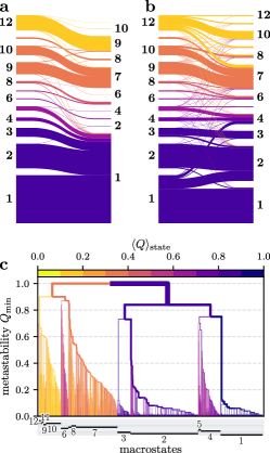
Figure 3: (a) Effects of using G-PCCA instead of MPP for the construction of macrostates. The Sankey diagrams compare the states obtained for the reference model (PCA/RDC/MPP, on the left) and the alternative model (PCA/RDC/G-PCCA, on the right). (b) Performance of the method combination tICA/$k$-means/MPP as revealed by the Sankey plot comparison to the reference model and (c) the MPP dendrogram.

Going back to using MPP for the construction of macrostates, we next study the performance of the microstate clustering by $k$-means (instead of RDC) in some more detail. Considering again the popular combination tICA/$k$-means, Fig. 3c shows the resulting MPP dendrogram, which reveals how the microstates are merged to macrostates. As expected from a purely geometrical clustering scheme, the $k\!=\!1000$ microstates generated by $k$-means (shown for $Q_{\rm min}\!=\!0$) typically exhibit significantly lower metastability than the density-based RDC microstates (Fig. 2a), and therefore are lumped already for low values of $Q_{\rm min}$. Moreover, $k$-means assigns a similar number of microstates to the native and the unfolded basins, while the free energy-based RDC exhibits only a few low-energy states in the native basin.

Comparing the resulting state partitioning to the reference, the Sankey diagram in Fig. 3d reveals that the combination tICA/$k$-means gives a closely related state description of the native basin, except for some reshuffling between states 1 and 2. On the other hand, we obtain only a single intermediate state and four unfolded states that are partitioned in a somewhat different way. This overall picture is similar for the combination tICA/RDC, while the combination PCA/$k$-means produces only 8 (instead of 12) metastable states (Fig. S1). With a GMRQ score of 2.83, 2.80, and 2.80 for tICA/$k$-means, tICA/RDC, and PCA/$k$-means, respectively, the implied timescales of all combinations are again very similar. Hence we find that the replacement of PCA by tICA and RDC by $k$-means overall yields similar dynamical models, although with possibly dissimilar spatial resolution of the free energy landscape. As a note of caution, however, we wish to stress that this conclusion rests heavily on the specific implementation of all used methods as well as on the choice of metaparameters (see Methods). Even more so, it is only valid if suitable features are chosen, as will be shown in the following.

2.3 Effect of feature selection

While the reference model employed native contacts determined via minimal distances, in the following we discuss several other popular choices, including Cartesian atom coordinates, C_α-distances, backbone dihedral angles, and a mixture of contacts and angles, see Fig. S2. If not noted otherwise, we use our standard workflow PCA/RDC/MPP and compare it to the popular combination tICA/$k$-means/MPP.

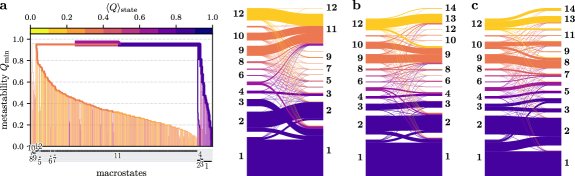
Figure 4: Effects of the choice of features, including (a) Cartesian coordinates, (b) selected C_α-distances, and (c) contacts combined with the backbone dihedral angle $\phi_{3}$. Shown are the Sankey plots for comparison to the reference states and the MPP dendrogram in case (a).

Cartesian atom coordinates

We first consider Cartesian coordinates of the C_α-atoms, which seem convenient as they directly reveal the three-dimensional structure of the system. To remove the overall translation and rotation of the trajectory, the coordinates of the rigid secondary structures (i.e., the three $\alpha$-helices of HP35) are typically aligned to a reference structure. As is well known,^{101, 102, 64} however, this procedure cannot entirely remove the overall rotation of a flexible system. Moreover, it has been shown that the calculation of the linear correlation underlying PCA and tICA is ill-defined for three-dimensional vectors, because the contributions in $x$, $y$ and $z$ direction depend spuriously on the relative orientation of the fluctuations.¹⁰³

Displaying the resulting MPP dendrogram and the Sankey plot for comparison to the reference states, Fig. 4a reveals the consequences of these issues. Most obviously, the MPP dendrogram shows that Cartesian coordinates cannot capture the hierarchical structure of the unfolded part of the free energy landscape, i.e., the unfolded basin is virtually structureless and represented by only a single state. Moreover, while the native basin is found to split up in several states, their contact representation reveals that the structures of these states are mixed instead of being well characterized, see Fig. S2a for further details. Reflected by a GMRQ score of 2.72, the first implied timescale of the model is too low by a factor 5, which adds to the conclusion that Cartesian-based MSMs are not suited to describe protein folding.⁶⁴ Interestingly, we find that the timescales improve considerably (GMRQ = 2.90) when we use tICA instead of PCA. Since tICA cannot correct for the mixing of overall and internal motion, however, the resulting state partitioning is still rather poor (Fig. S2a). Hence, we add as a note of caution that variational feature selection can rate Cartesian-based MSMs deceivingly high,⁶⁸ although they may not correctly account for the structural evolution during folding.

C_α-distances

To avoid problems associated with the mixing of overall and internal motion, internal coordinates are commonly chosen as features. An obvious option are interresidue distances, such as C_α-distances and contact distances. While the appropriate identification of contacts via minimal atom distances requires some effort (see Sec. 2.1), distances between C_α atoms are readily extracted from an MD trajectory and may be used as an approximate definition of an interresidue contact. This is achieved by employing a distance cutoff of 8 Å, ⁷⁶ and by requesting a minimum persistence probability of 30 % in order to focus on native contacts (see Sec. 2.1).

Showing the resulting MPP dendrogram and the Sankey plot, Fig. 4b reveals that the C_α-distance-based model reproduces faithfully the states of the native basin, while the unfolded part of the energy landscape matches only roughly the reference results. In particular, we find that the two main unfolded states are structurally not well defined (Fig. S2b), whereas the partially and completely unfolded states of the reference model clearly differ by the existence of contacts in clusters 3 and 4 (Fig. 2b). This is because the approximate contact definition is sufficient to distinguish well-defined native states, but is not suited to partition the structurally very heterogeneous unfolded basin. As a consequence, we find that the implied timescales are significantly reduced, yielding a GMRQ score of 2.67. While the latter issue can be improved by using tICA instead of PCA (resulting in GMRQ = 2.89), tICA does not yield a better state partitioning of the unfolded basin.

Besides using selected C_α-distances to approximate interresidue contacts, we can also simply employ all $N(N\!-\!1)/2$ C_α-distances as features for an MSM. Although this results in a highly redundant feature set whose dimension increases rapidly for larger systems, the choice is quite popular as it is straightforward and requires no metaparameters.⁶⁸ Somewhat surprisingly, though, the resulting MPP dendrogram and the Sankey plot in Fig. S2c reveals that the state partitioning deteriorates dramatically when we use all (instead of selected) C_α-distances. Similar as found above for Cartesian atom coordinates, the unfolded basin is virtually structureless and represented by only a single state, while the native basin consists of three states, whose structures are mixed. A MoSAIC analysis reveals the existence of a number of clusters, whose many redundant distances and the associated ambiguity hamper an accurate structural characterization. Moreover, the first implied timescale of the model is too low by a factor 5, giving a poor GMRQ score of 2.47. While timescales –and to some extent also the state splitting– can be improved by using the combination tICA/$k$-means instead of PCA/RDC, the various states are structurally still poorly defined (Fig. S2c).

Backbone dihedral angles

In Ref. 70 we compared in detail the virtues and shortcomings of using backbone dihedral angles instead of interresidue contacts. While dihedral angles are readily obtained from the MD trajectory, they require an appropriate treatment of their periodicity ^{104, 105, 106} (e.g., by using maximal-gap shifted¹⁰⁵ ($\phi,\psi$) dihedral angles) and necessitate the exclusion of uncorrelated motion of the terminal ends. With $\psi$-angles reflecting the helicity of the protein and $\phi$-angles accounting for potential left-to-right handed transitions (e.g., in flexible loops), backbone dihedral angles report directly on the local secondary structure. This proves advantageous for the modeling of the conformational states in the native basin of HP35, which interestingly can be well approximated by a single angle, $\phi_{3}$. However, dihedral angles account only indirectly for the formation of tertiary structure during folding, which yields a low-resolution description of the unfolded basin, hampers the precise modeling of the folding transition, and therefore results in shorter implied timescales.⁷⁰

While the discussion above indicates that interresidue contacts are better suited for the description of folding, it also suggests combining the best of two worlds and use contacts to describe the formation of tertiary structure, and include the single angle $\phi_{3}$ to accurately account for the substates of the native basin. (We note in passing that various types of feature can be combined in the analysis, because we normalize all features before dimensionality reduction.) Regarding the state partitioning of the native basin, the resulting Sankey plot is found to differ only minor from contacts-only reference model (Fig. 4c), i.e., there is no benefit here. Interestingly, though, the unfolded part of the free energy landscape is described with high resolution and shows numerous substates, which might represent an improvement upon the reference model (Fig. S2d).

2.4 Effect of temperature

An alternative way to assess the robustness of a model is studying to what extent it accounts for a variation of the input data. As an example, we consider a folding trajectory of HP35 at 370 K (instead of 360 K), which was also obtained by Piana et al.⁴² Since they otherwise applied identical simulation conditions, we use the same 42 minimal-distance contacts as features. Showing the time evolution of the fraction of native contacts, Fig. S3a reveals that due to the increased temperature only about half of the trajectory (instead of two thirds) populates the native basin, and that the mean folding time is reduced by 20%. While these results are expected, it is less clear how the free energy landscape and the state partitioning changes. Using our standard workflow PCA/RDC/MPP, the 370 K trajectory results in virtually the same five native states, while the unfolded part of the free energy landscape collapses into a single unfolded state (Fig. S3b). Likewise, the combination tICA/$k$-means/MPP splits up the unfolded basin in four states (similar to the ones found for 360 K) and also yields a single unfolded state (Fig. S3c). In both cases, the implied timescales are reduced by about 40% with respect to the results at 360 K. Hence, the overall trends shown by the two contact-based MSMs appear to draw a consistent picture of the temperature dependence of the system.

2.5 Exploring the method space

To provide an overview of all considered methods and features, we now introduce three qualitative scoring functions. While the dynamical quality of an MSM can be readily assessed via the GMRQ score³¹ reflecting the implied timescales, it is less straightforward to characterize the structural quality of a state partitioning. Here two complementary measures are employed: On the one hand, we use the Shannon entropy $H=-\sum_{j}p_{j}\ln p_{j}$ of the state populations $p_{j}$, which is maximal for equally distributed $p_{j}$. Hence, a high value of $H$ means that the majority of states is well populated, which we favor over partitionings with a few highly and many lowly populated states. On the other hand, we consider the Davies-Bouldin index ¹⁰⁷ which is a well-established descriptor of the similarity of clusters (see Methods), and is to be minimized to ensure structurally distinct states. To obtain easy-to-compare quantities that all should be maximal, we consider $\Delta$DBI = DBI${}_{\rm max}-$DBI.

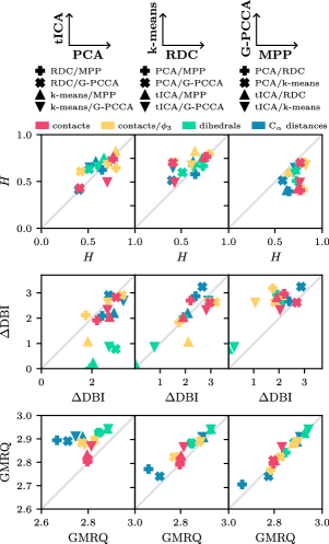
Figure 5: Comparison of various methods and features, showing (top) the normalized entropy score $H$, (middle) the Davies-Bouldin index $\Delta$DBI = DBI${}_{\rm max}-$DBI, and (bottom) the timescale score GMRQ, which all should be maximized.

Comparing various method combinations of the MSM workflow, Fig. 5 shows these three scoring functions as obtained for various features, including contacts, contacts/$\phi_{3}$, backbone dihedral angles, and selected C_α-distances. We begin with the comparison of PCA and tICA, which as expected shows that tICA clearly improves the timescale score, in particular for dihedrals. While the entropy score shows no clear trend, the Davies-Bouldin index reveals the opposite picture, i.e., PCA generally obtains better scores, and the tICA results for dihedrals indicates a significant structural overlap of the resulting states. This well-know effect⁶⁵ is caused by left to right-handed transitions along the $\phi$ dihedral angles, which represent slow but functionally irrelevant motions, because the left-handed states are hardly populated. Nevertheless, these irrelevant motions are favored by tICA (because they are slow) and therefore lead to structurally nonsensical states.⁶⁴

When we compare RDC and $k$-means clustering (middle column of Fig. 5), no clear trend is apparent, which is in line with our findings above. While timescales seem to be sightly better reproduced by $k$-means, the situation is diverse for the two structural scores, where sometimes RDC and some other time $k$-means performs better. Comparing MPP and G-PCCA (right column of Fig. 5), the resulting timescales are virtually identical. Since G-PCCA tends to result in a few well-populated main states, the entropy score favors MPP, while the Davies-Bouldin index favors G-PCCA because these few main states are clearly distinct.

3 Conclusions

To validate the contact-based MSM of Ref. 70, we have considered various combinations of features, dimensionality reduction methods and clustering schemes. Using minimal-distance contacts as features, we have found that –depending on the specific combination– we get MSMs with quite similar implied timescales but possibly different partitionings of the free energy landscape. While G-PCCA was shown to generally achieve lower spatial resolution than MPP, the usage of tICA instead of PCA and $k$-means instead of RDC for the most part resulted in overall comparable state partitionings. In this way, the overall consistence of the reference model with the alternative method combinations confirms our initial proposition that the folding of HP35 exhibits a hierarchical structure of the free energy landscape, where both the native and the unfolded basin split up in various well populated metastable states, and where a few lowly populated intermediate states exist.

Hence, our study has demonstrated that for a given MD trajectory several sets of metastable states with different structural ensembles may co-exist, and that it is not straightforward to assess which state partitioning is superior. As a consequence, the above results also indicate to what extent a reference or benchmark MSM may be defined for a high-dimensional biomolecular process such as the folding of HP35. While our reference model is certainly not the only or the best one, it nonetheless satisfies the above formulated criteria of achieving sufficient structural detail to resolve the various metastable states and folding pathways of HP35, and of yielding sufficiently long implied timescales to represent a correct Markovian model.

Our study of various methods and features has also revealed which parts of the MSM workflow matter most for the considered problem. Notably, we have found that standard methods of dimensionality reduction (like PCA and tICA), microstate clustering (such as RDC and $k$-means), and macrostate clustering (such as MPP and PCCA) typically give reasonable MSMs, if they are applied with caution (see Methods), and if appropriate features are employed. Using improper features, the MSM necessarily fails, regardless of what methods are subsequently used: ’garbage in, garbage out’. For example, we have shown that Cartesian atom coordinates completely fail to describe the hierarchical nature of the unfolded region, due to the mixing of internal and overall motion. On the other hand, we have found that contact-based MSMs quite reliably produce good and robust timescales and state partitionings for a variety of methods.

The discussion above points out the importance of the choice and the pre-selection of suitable features. While the basic idea is to choose internal coordinates that account for the mechanistic origin of the studied process, it also means to carefully exclude irrelevant and deceiving motions from the analysis. To this end, we recently proposed the correlation analysis MoSAIC,⁶⁷ which aims to discriminate collective motions underlying functional dynamics from uncorrelated motion. Applied to dihedral angles, for example, MoSAIC readily identifies slow uncorrelated motion along $\phi$ angles,⁷⁰ which would deceive timescale optimizing approaches such as tICA (see the discussion of tICA in Fig. 5). Moreover, we have shown that restricting ourselves to selected C_α-distances that approximate interresidue contacts significantly improves the signal-to-noise ratio, such that details of the free energy landscape can be resolved. While we are confident that the merits of feature selection are just as important for the modeling of much larger systems than HP35, this remains to be proven in future work.

4 Methods

MD details. This work is based on the $300\text{\,}\mathrm{\SIUnitSymbolMicro s}$-long MD simulation ($1.5\times 10^{6}$ data points) of the fast folding Lys24Nle/Lys29Nle mutant of HP35 (pdb 2F4K, Ref. 46) at $T=$360\text{\,}\mathrm{K}$$ by Piana et al.,⁴² using the Amber ff99SB*-ILDN force-field ^{108, 109, 110} and the TIP3P water model.¹¹¹

Feature selection. Features include contacts determined via minimal distances and via C_α-distances, Cartesian atom coordinates, all C_α-distances, backbone dihedral angles, and a mixture of contacts and angles. Their computation is defined in the main text. To achieve a pre-selection of features, we employed the Python package MoSAIC⁶⁷ (“Molecular Systems Automated Identification of Cooperativity”). It is based on a community detection technique called Leiden clustering¹¹², which employs the constant Potts model as objective function.

Dimensionality reduction. We focused on two simple and widely used linear methods, PCA and tICA, which produce smoothly varying free energy landscapes that facilitate the subsequent clustering. PCA was employed as implemented in the open source software FastPCA, ¹⁰⁵. tICA was employed as implemented in PyEmma, ¹⁵ using $\tau_{\text{lag}}=10\,$ns and scaling the eigenvectors by their eigenvalues.⁸¹ Including the first five components in both cases, subsequently a Gaussian low-pass filter with a standard deviation of $\sigma=2\,$ns was employed.

Clustering. RDC⁷⁷ was implemented in the open source software Clustering, ⁶⁵ using a hypersphere radius $R=0.124$ that equals the lumping radius. MPP was implemented as described in Ref. 78. Alternatively, we employed the mini-batch $k$-means algorithm⁹⁸ in combination with the $k$-means++ initialization,⁹⁹ as implemented by Scikit-Learn.¹⁰⁰ We used $k=1000$, a batch size of 5120 frames, 100 random initial configurations, and a minimum (maximum) of $10^{3}$ ($10^{6}$) iteration steps. These relatively high numbers of configurations and iterations are required to obtain reproducible results from $k$-means, which can be compared to the deterministic RDC method. G-PCCA represents an extension of the well-established PCCA+ approach⁹³ that is implemented in PyEmma ¹⁵ and MSMBuilder.¹⁶

Analysis. All analyses shown in this paper were performed using our open-source Python package msmhelper.¹¹³ To facilitate the reproduction and analysis of our results for the reference model, we furthermore provide trajectories of all intermediate steps.

The Davies-Bouldin index for $N$ macrostates is defined by ¹⁰⁷

DBI $$=\frac{1}{N}\sum_{i=1}^{N}\max_{i\neq j}\left(\frac{s_{i}+s_{j}}{r_{ij}}\right),$$

where $s_{i}=\langle|\boldsymbol{x}-\langle\boldsymbol{x}\rangle_{i}|\rangle_{i}$ is the average distance between each point of a state $i$ and the centroid of that cluster, $r_{ij}=|\langle\boldsymbol{x}\rangle_{i}-\langle\boldsymbol{x}\rangle_{j}|$ is the distance between cluster centroids $i$ and $j$, and $\boldsymbol{x}$ represents the 42 contact distances.

Computational effort. The complete workflow of the reference MSM took 16 min CPU time on a standard desktop computer, except for contact definition which additionally took about 2 h. As discussed in Ref. 70, the treatment of proteins with $10^{3}$ residues is estimated to require in total a few CPU days, which is negligible compared to the time required for the MD simulations.

Acknowledgment

The authors thank Georg Diez, Matthias Post and Steffen Wolf for helpful comments and discussions, as well as D. E. Shaw Research for sharing their trajectories of HP35. This work has been supported by the Deutsche Forschungsgemeinschaft (DFG) within the framework of the Research Unit FOR 5099 ”Reducing complexity of nonequilibrium systems” (project No. 431945604), the High Performance and Cloud Computing Group at the Zentrum für Datenverarbeitung of the University of Tübingen and the Rechenzentrum of the University of Freiburg, the state of Baden-Württemberg through bwHPC and the DFG through Grant Nos. INST 37/935-1 FUGG (RV bw16I016) and INST 39/963-1 FUGG (RV bw18A004).

Data Availability Statement

The simulation data and all intermediate results for our reference model, including our software packages MoSAIC,⁶⁷ FastPCA,¹⁰⁵ Clustering⁷⁷ and msmhelper¹¹³ and detailed descriptions to reproduce all steps of the analyses, can be downloaded from https://github.com/moldyn/HP35. In particular, we provide trajectories ($300\text{\,}\mathrm{\SIUnitSymbolMicro s}$ long, $1.5\times 10^{6}$ data points) of (1) the contact distances, (2) the maximal-gap shifted dihedral angles, (3) the resulting principal components, and (4) the resulting micro- and macrostates.

Supporting Information

Figure S1 shows for all eight considered combinations of methods (PCA vs. tICA, RDC vs. $k$-means, and MPP vs. G-PCCA) the MPP dendrogram, the contact characterization of the metastable states, a Sankey diagram to compare to the reference states, and the implied timescales. Figure S2 shows these quantities for various features including Cartesian atom coordinates, selected and all C_α-distances, and contacts/$\phi_{3}$. Figure S3 shows results obtained for a folding trajectory at 370 K.

References

- Berendsen 2007 Berendsen, H. J. C. Simulating the Physical World; Cambridge University Press: Cambridge, 2007
- Lange and Grubmüller 2006 Lange, O. F.; Grubmüller, H. Collective Langevin dynamics of conformational motions in proteins. J. Chem. Phys. 2006, 124, 214903
- Hegger and Stock 2009 Hegger, R.; Stock, G. Multidimensional Langevin modeling of biomolecular dynamics. J. Chem. Phys. 2009, 130, 034106
- Ayaz et al. 2021 Ayaz, C.; Tepper, L.; Brünig, F. N. et al. Non-Markovian modeling of protein folding. Proc. Natl. Acad. Sci. USA 2021, 118, e2023856118
- Chodera et al. 2007 Chodera, J. D.; Singhal, N.; Pande, V. S. et al. Automatic discovery of metastable states for the construction of Markov models of macromolecular dynamics. J. Chem. Phys. 2007, 126, 155101
- Noé et al. 2007 Noé, F.; Horenko, I.; Schütte, C. et al. Hierarchical analysis of conformational dynamics in biomolecules: Transition networks of metastable states. J. Chem. Phys. 2007, 126, 155102
- Buchete and Hummer 2008 Buchete, N.-V.; Hummer, G. Coarse master equations for peptide folding dynamics. J. Phys. Chem. B 2008, 112, 6057–6069
- Prinz et al. 2011 Prinz, J.-H.; Wu, H.; Sarich, M. et al. Markov models of molecular kinetics: generation and validation. J. Chem. Phys. 2011, 134, 174105
- Bowman et al. 2013 Bowman, G. R.; Pande, V. S.; Noé, F. An Introduction to Markov State Models; Springer: Heidelberg, 2013
- Wang et al. 2018 Wang, W.; Cao, S.; Zhu, L. et al. Constructing Markov State Models to elucidate the functional conformational changes of complex biomolecules. WIREs Comp. Mol. Sci. 2018, 8, e1343
- Husic and Pande 2018 Husic, B. E.; Pande, V. S. Markov State Models: From an Art to a Science. J. Am. Chem. Soc. 2018, 140, 2386–2396
- Noé and Rosta 2019 Noé, F.; Rosta, E. Markov Models of Molecular Kinetics. J. Chem. Phys. 2019, 151, 190401
- Noe et al. 2009 Noe, F.; Schütte, C.; Vanden-Eijnden, E. et al. Constructing the Full Ensemble of Folding Pathways from Short Off-Equilibrium Simulations. Proc. Natl. Acad. Sci. USA 2009, 106, 19011–19016
- Bowman et al. 2010 Bowman, G. R.; Ensign, D. L.; Pande, V. S. Enhanced modeling via network theory: Adaptive sampling of Markov state models. J. Chem. Theory Comput. 2010, 6, 787–94
- Scherer et al. 2015 Scherer, M. K.; Trendelkamp-Schroer, B.; Paul, F. et al. PyEMMA 2: A Software Package for Estimation, Validation, and Analysis of Markov Models. J. Chem. Theory Comput. 2015, 11, 5525
- Beauchamp et al. 2011 Beauchamp, K. A.; Bowman, G. R.; Lane, T. J. et al. MSMBuilder2: Modeling Conformational Dynamics on the Picosecond to Millisecond Scale. J. Chem. Theory Comput. 2011, 7, 3412–3419
- Zwanzig 1983 Zwanzig, R. From classical dynamics to continuous time random walks. J. Stat. Phys. 1983, 30, 255–262
- Sarich et al. 2010 Sarich, M.; Noé, F.; Schütte, C. On the Approximation Quality of Markov State Models. SIAM Multiscale Model. Simul. 2010, 8, 1154–1177
- Knoch and Speck 2017 Knoch, F.; Speck, T. Nonequilibrium Markov state modeling of the globule-stretch transition. Phys. Rev. E 2017, 95, 012503
- Paul et al. 2019 Paul, F.; Wu, H.; Vossel, M. et al. Identification of kinetic order parameters for non-equilibrium dynamics. J. Chem. Phys. 2019, 150, 164120
- Hartich and Godec 2021 Hartich, D.; Godec, A. Emergent Memory and Kinetic Hysteresis in Strongly Driven Networks. Phys. Rev. X 2021, 11, 041047
- Wu et al. 2016 Wu, H.; Paul, F.; Wehmeyer, C. et al. Multiensemble Markov models of molecular thermodynamics and kinetics. Proc. Natl. Acad. Sci. USA 2016, 113, E3221–E3230
- Schütte et al. 2011 Schütte, C.; Noé, F.; Lu, J. et al. Markov state models based on milestoning. J. Chem. Phys. 2011, 134, 204105
- Jain and Stock 2014 Jain, A.; Stock, G. Hierarchical folding free energy landscape of HP35 revealed by most probable path clustering. J. Phys. Chem. B 2014, 118, 7750 – 7760
- Lemke and Keller 2016 Lemke, O.; Keller, B. G. Density-based cluster algorithms for the identification of core sets. J. Chem. Phys. 2016, 145, 164104
- Cao et al. 2020 Cao, S.; Montoya-Castillo, A.; Wang, W. et al. On the advantages of exploiting memory in Markov state models for biomolecular dynamics. J. Chem. Phys. 2020, 153, 014105
- Suarez et al. 2021 Suarez, E.; Wiewiora, R. P.; Wehmeyer, C. et al. What Markov State Models Can and Cannot Do: Correlation versus Path-Based Observables in Protein-Folding Models. J. Chem. Theory Comput. 2021, 17, 3119–3133
- Dominic et al. 2023 Dominic, A. J.; Sayer, T.; Cao, S. et al. Building insightful, memory-enriched models to capture long-time biochemical processes from short-time simulations. Proc. Natl. Acad. Sci. USA 2023, 120, e2221048120
- Nüske et al. 2014 Nüske, F.; Keller, B. G.; Perez-Hernández, G. et al. Variational Approach to Molecular Kinetics. J. Chem. Theory Comput. 2014, 10, 1739–1752
- Wu and Noé 2020 Wu, H.; Noé, F. Learning Markov Processes from Time Series Data. J. Nonlinear. Sci. 2020, 30, 23–66
- McGibbon and Pande 2015 McGibbon, R. T.; Pande, V. S. Variational cross-validation of slow dynamical modes in molecular kinetics. J. Chem. Phys. 2015, 142, 124105
- Husic et al. 2016 Husic, B. E.; McGibbon, R. T.; Sultan, M. M. et al. Optimized parameter selection reveals trends in Markov state models for protein folding. J. Chem. Phys. 2016, 145, 194103
- Vroylandt et al. 2022 Vroylandt, H.; Goudenège, L.; Monmarché, P. et al. Likelihood-based non-Markovian models from molecular dynamics. Proc. Natl. Acad. Sci. USA 2022, 119, e2117586119
- 34 This was one of the main conclusions of the 2019 CECAM workshop in Paris on "Learning the Collective Variables of Biomolecular Processes" organized by L. Delemotte, J. Hénin, T. Leliévre and G. Stock
- Wang et al. 2020 Wang, Y.; Lamim Ribeiro, J. M.; Tiwary, P. Machine learning approaches for analyzing and enhancing molecular dynamics simulations. Curr. Opin. Struct. Biol. 2020, 61, 139–145
- Fleetwood et al. 2020 Fleetwood, O.; Kasimova, M. A.; Westerlund, A. M. et al. Molecular Insights from Conformational Ensembles via Machine Learning. Biophys. J. 2020, 118, 765–780
- Glielmo et al. 2021 Glielmo, A.; Husic, B. E.; Rodriguez, A. et al. Unsupervised Learning Methods for Molecular Simulation Data. Chem. Rev. 2021, 121, 9722–9758
- Konovalov et al. 2021 Konovalov, K. A.; Unarta, I. C.; Cao, S. et al. Markov State Models to Study the Functional Dynamics of Proteins in the Wake of Machine Learning. JACS Au 2021, 1, 1330–1341
- 39 Aiming at a rigorous calculation of reaction coordinates, however, besides () additional internal coordinates were suggested, see, e.g., Refs. 40, 41
- Bolhuis et al. 2000 Bolhuis, P. G.; Dellago, C.; Chandler, D. Reaction coordinates of biomolecular isomerization. Proc. Natl. Acad. Sci. USA 2000, 97, 5877 – 5882
- Wu et al. 2022 Wu, S.; Li, H.; Ma, A. A Rigorous Method for Identifying a One-Dimensional Reaction Coordinate in Complex Molecules. J. Chem. Theory Comput. 2022, 18, 2836–2844
- Piana et al. 2012 Piana, S.; Lindorff-Larsen, K.; Shaw, D. E. Protein folding kinetics and thermodynamics from atomistic simulation. Proc. Natl. Acad. Sci. USA 2012, 109, 17845–17850
- McKnight et al. 1997 McKnight, C. J.; Matsudaira, P. T.; Kim, P. S. NMR structure of the 35-residue villin headpiece subdomain. Nat. Struct. Biol. 1997, 4, 180 – 184
- Kubelka et al. 2003 Kubelka, J.; Eaton, W. A.; Hofrichter, J. Experimental tests of villin subdomain folding simulations. J. Mol. Biol. 2003, 329, 625–630
- Kubelka et al. 2004 Kubelka, J.; Hofrichter, J.; Eaton, W. A. The protein folding "speed limit". Curr. Opin. Struct. Biol. 2004, 14, 76 – 88
- Kubelka et al. 2006 Kubelka, J.; Chiu, T. K.; Davies, D. R. et al. Sub-microsecond protein folding. J. Mol. Biol. 2006, 359, 546–553
- Brewer et al. 2007 Brewer, S.; Song, B.; Raleigh, D. et al. Residue Specific Resolution of Protein Folding Dynamics Using Isotope-Edited Infrared Temperature Jump Spectroscopy. Biochem. 2007, 46, 3279–3285
- Kubelka et al. 2008 Kubelka, J.; Henry, E. R.; Cellmer, T. et al. Chemical, physical, and theoretical kinetics of an ultrafast folding protein. Proc. Natl. Acad. Sci. USA 2008, 105, 18655–18662
- Reiner et al. 2010 Reiner, A.; Henklein, P.; Kiefhaber, T. An unlocking/relocking barrier in conformational fluctuations of villin headpiece subdomain. Proc. Natl. Acad. Sci. USA 2010, 107, 4955 – 4960
- Chung et al. 2011 Chung, J. K.; Thielges, M. C.; Fayer, M. D. Dynamics of the folded and unfolded villin headpiece (HP35) measured with ultrafast 2D IR vibrational echo spectroscopy. Proc. Natl. Acad. Sci. USA 2011, 108, 3578–3583
- Serrano et al. 2012 Serrano, A. L.; Bilsel, O.; Gai, F. Native State Conformational Heterogeneity of HP35 Revealed by Time-Resolved FRET. J. Phys. Chem. B 2012, 116, 10631–10638
- Eaton 2021 Eaton, W. A. Modern Kinetics and Mechanism of Protein Folding: A Retrospective. J. Phys. Chem. B 2021, 125, 3452–3467
- Duan and Kollman 1998 Duan, Y.; Kollman, P. A. Pathways to a protein folding intermediate observed in a 1-microsecond simulation in aqueous solution. Science 1998, 282, 740–744
- Snow et al. 2002 Snow, C. D.; Nguyen, H.; Pande, V. S. et al. Absolute comparison of simulated and experimenta protein folding dynamics. Nature (London) 2002, 420, 102
- Fernández et al. 2003 Fernández, A.; Shen, M. Y.; Colubri, A. et al. Large-scale context in protein folding: villin headpiece. Biochem. 2003, 42, 664–671
- Lei et al. 2007 Lei, H.; Wu, C.; Liu, H. et al. Folding free-energy landscape of villin headpiece subdomain from molecular dynamics simulations. Proc. Natl. Acad. Sci. USA 2007, 104, 4925–4930
- Ensign et al. 2007 Ensign, D. L.; Kasson, P. M.; Pande, V. S. Heterogeneity even at the speed limit of folding: large-scale molecular dynamics study of a fast-folding variant of the villin headpiece. J. Mol. Biol. 2007, 374, 806–816
- Rajan et al. 2010 Rajan, A.; Freddolino, P. L.; Schulten, K. Going beyond clustering in MD trajectory analysis: an application to villin headpiece folding. PLoS One 2010, 5, e9890
- Shaw et al. 2010 Shaw, D. E.; Maragakis, P.; Lindorff-Larsen, K. et al. Atomic-Level Characterization of the Structural Dynamics of Proteins. Science 2010, 330, 341–346
- Beauchamp et al. 2012 Beauchamp, K. A.; McGibbon, R.; Lin, Y.-S. et al. Simple few-state models reveal hidden complexity in protein folding. Proc. Natl. Acad. Sci. USA 2012, 109, 17807 – 17813
- Sormani et al. 2020 Sormani, G.; Rodriguez, A.; Laio, A. Explicit Characterization of the Free-Energy Landscape of a Protein in the Space of All Its Cα Carbons. J. Chem. Theory Comput. 2020, 16, 80–87
- Chong and Ham 2021 Chong, S.-H.; Ham, S. Time-dependent communication between multiple amino acids during protein folding. Chem. Sci. 2021, 12, 5944–5951
- Ernst et al. 2015 Ernst, M.; Sittel, F.; Stock, G. Contact- and distance-based principal component analysis of protein dynamics. J. Chem. Phys. 2015, 143, 244114
- Sittel and Stock 2018 Sittel, F.; Stock, G. Perspective: Identification of Collective Coordinates and Metastable States of Protein Dynamics. J. Chem. Phys. 2018, 149, 150901
- Nagel et al. 2019 Nagel, D.; Weber, A.; Lickert, B. et al. Dynamical coring of Markov state models. J. Chem. Phys. 2019, 150, 094111
- Nagel et al. 2020 Nagel, D.; Weber, A.; Stock, G. MSMPathfinder: Identification of pathways in Markov state models. J. Chem. Theory Comput. 2020, 16, 7874 – 7882
- Diez et al. 2022 Diez, G.; Nagel, D.; Stock, G. Correlation-based feature selection to identify functional dynamics in proteins. J. Chem. Theory Comput. 2022, 18, 5079 – 5088
- Scherer et al. 2019 Scherer, M. K.; Husic, B. E.; Hoffmann, M. et al. Variational selection of features for molecular kinetics. J. Chem. Phys. 2019, 150, 194108
- Ravindra et al. 2020 Ravindra, P.; Smith, Z.; Tiwary, P. Automatic mutual information noise omission (AMINO): generating order parameters for molecular systems. Mol. Syst. Des. Eng. 2020, 5, 339–348
- Nagel et al. 2023 Nagel, D.; Sartore, S.; Stock, G. Selecting Features for Markov Modeling: A Case Study on HP35. J. Chem. Theory Comput. 2023, 19, 3391–3405
- Jacomy et al. 2014 Jacomy, M.; Venturini, T.; Heymann, S. et al. ForceAtlas2, a Continuous Graph Layout Algorithm for Handy Network Visualization Designed for the Gephi Software. PLOS ONE 2014, 9, 1–12
- Sali et al. 1994 Sali, A.; Shakhnovich, E.; Karplus, M. How does a protein fold? Nature (London) 1994, 369, 248 – 251
- Wolynes et al. 1995 Wolynes, P. G.; Onuchic, J. N.; Thirumalai, D. Navigating the Folding Routes. Science 1995, 267, 1619–1620
- Best et al. 2013 Best, R. B.; Hummer, G.; Eaton, W. A. Native contacts determine protein folding mechanisms in atomistic simulations. Proc. Natl. Acad. Sci. USA 2013, 110, 17874–17879
- Best and Hummer 2010 Best, R. B.; Hummer, G. Coordinate-dependent diffusion in protein folding. Proc. Natl. Acad. Sci. USA 2010, 107, 1088 – 1093
- Yao et al. 2019 Yao, X.-Q.; Momin, M.; Hamelberg, D. Establishing a Framework of Using Residue–Residue Interactions in Protein Difference Network Analysis. J. Chem. Inf. Model. 2019, 59, 3222–3228
- Sittel and Stock 2016 Sittel, F.; Stock, G. Robust Density-Based Clustering to Identify Metastable Conformational States of Proteins. J. Chem. Theory Comput. 2016, 12, 2426–2435
- Jain and Stock 2012 Jain, A.; Stock, G. Identifying metastable states of folding proteins. J. Chem. Theory Comput. 2012, 8, 3810 – 3819
- 79 In fact, these conditions produced 13 (instead of 12) contacts-based states. Since the additional state 13 (on the very left side of the dendrogram) is completely unfolded just like state 12, however, we simply merged them into a single state when we discuss folding70
- Hummer and Szabo 2015 Hummer, G.; Szabo, A. Optimal Dimensionality Reduction of Multistate Kinetic and Markov-State Models. J. Phys. Chem. B 2015, 119, 9029–9037
- Noé and Clementi 2015 Noé, F.; Clementi, C. Kinetic Distance and Kinetic Maps from Molecular Dynamics Simulation. J. Chem. Theory Comput. 2015, 11, 5002–5011
- Rohrdanz et al. 2013 Rohrdanz, M. A.; Zheng, W.; Clementi, C. Discovering Mountain Passes via Torchlight: Methods for the Definition of Reaction Coordinates and Pathways in Complex Macromolecular Reactions. Annu. Rev. Phys. Chem. 2013, 64, 295–316
- Fiorin et al. 2013 Fiorin, G.; Klein, M. L.; Hénin, J. Using collective variables to drive molecular dynamics simulations. Mol. Phys. 2013, 111, 3345 – 3362
- Rodriguez et al. 2018 Rodriguez, A.; d’Errico, M.; Facco, E. et al. Computing the Free Energy without Collective Variables. J. Chem. Theory Comput. 2018, 14, 1206–1215
- Chen et al. 2018 Chen, W.; Tan, A. R.; Ferguson, A. L. Collective variable discovery and enhanced sampling using autoencoders: Innovations in network architecture and error function design. J. Chem. Phys. 2018, 149, 072312
- Lemke and Peter 2019 Lemke, T.; Peter, C. EncoderMap: Dimensionality Reduction and Generation of Molecule Conformations. J. Chem. Theory Comput. 2019, 15, 1209–1215
- Wang et al. 2019 Wang, Y.; Ribeiro, J.; Tiwary, P. Past–future information bottleneck for sampling molecular reaction coordinate simultaneously with thermodynamics and kinetics. Nat. Commun. 2019, 10, 3573
- Keller et al. 2010 Keller, B.; Daura, X.; van Gunsteren, W. F. Comparing geometric and kinetic cluster algorithms for molecular simulation data. J. Chem. Phys. 2010, 132, 074110
- Rodriguez and Laio 2014 Rodriguez, A.; Laio, A. Clustering by fast search and find of density peaks. Science 2014, 344, 1492–1496
- Song et al. 2017 Song, L.; Lizhe, Z.; Kit, S. F. et al. Adaptive partitioning by local density-peaks: An efficient density-based clustering algorithm for analyzing molecular dynamics trajectories. J. Comput. Chem. 2017, 38, 152–160
- Westerlund and Delemotte 2019 Westerlund, A. M.; Delemotte, L. InfleCS: Clustering Free Energy Landscapes with Gaussian Mixtures. J. Chem. Theory Comput. 2019, 15, 6752–6759
- Bowman et al. 2013 Bowman, G. R.; Meng, L.; Huang, X. Quantitative comparison of alternative methods for coarse-graining biological networks. J. Chem. Phys. 2013, 139, 121905
- Röblitz and Weber 2013 Röblitz, S.; Weber, M. Fuzzy spectral clustering by PCCA+: application to Markov state models and data classification. Adv. Data Anal. Classi. 2013, 7, 147–179
- Reuter et al. 2019 Reuter, B.; Fackeldey, K.; Weber, M. Generalized Markov modeling of nonreversible molecular kinetics. J. Chem. Phys. 2019, 150, 174103
- Martini et al. 2017 Martini, L.; Kells, A.; Covino, R. et al. Variational Identification of Markovian Transition States. Phys. Rev. X 2017, 7, 031060
- Wang et al. 2018 Wang, W.; Liang, T.; Sheong, F. K. et al. An efficient Bayesian kinetic lumping algorithm to identify metastable conformational states via Gibbs sampling. J. Phys. Chem. 2018, 149, 072337
- Perez-Hernandez et al. 2013 Perez-Hernandez, G.; Paul, F.; Giorgino, T. et al. Identification of slow molecular order parameters for Markov model construction. J. Chem. Phys. 2013, 139, 015102
- Sculley 2010 Sculley, D. Web-scale k-means clustering. Proceedings of the 19th international conference on World wide web. 2010; pp 1177–1178
- Arthur and Vassilvitskii 2007 Arthur, D.; Vassilvitskii, S. K-means++ the advantages of careful seeding. Proceedings of the eighteenth annual ACM-SIAM symposium on Discrete algorithms. 2007; pp 1027–1035
- Pedregosa et al. 2011 Pedregosa, F.; Varoquaux, G.; Gramfort, A. et al. Scikit-learn: Machine Learning in Python. J. Mach. Learn. Res. 2011, 12, 2825–2830
- Mu et al. 2005 Mu, Y.; Nguyen, P. H.; Stock, G. Energy Landscape of a Small Peptide Revealed by Dihedral Angle Principal Component Analysis. Proteins 2005, 58, 45 – 52
- Sittel et al. 2014 Sittel, F.; Jain, A.; Stock, G. Principal component analysis of molecular dynamics: On the use of Cartesian vs. internal coordinates. J. Chem. Phys. 2014, 141, 014111
- Lange and Grubmüller 2006 Lange, O. F.; Grubmüller, H. Generalized Correlation for Biomolecular Dynamics. Proteins 2006, 62, 1053–1061
- Altis et al. 2007 Altis, A.; Nguyen, P. H.; Hegger, R. et al. Dihedral angle principal component analysis of molecular dynamics simulations. J. Chem. Phys. 2007, 126, 244111
- Sittel et al. 2017 Sittel, F.; Filk, T.; Stock, G. Principal component analysis on a torus: Theory and application to protein dynamics. J. Chem. Phys. 2017, 147, 244101
- Zoubouloglou et al. 2022 Zoubouloglou, P.; García-Portugués, E.; Marron, J. S. Scaled Torus Principal Component Analysis. J. Comput. Graph. Stat. 2022, 0, 1–12
- Davies and Bouldin 1979 Davies, D. L.; Bouldin, D. W. A Cluster Separation Measure. IEEE PAMI 1979, PAMI-1, 224 – 227
- Hornak et al. 2006 Hornak, V.; Abel, R.; Okur, A. et al. Comparison of multiple Amber force fields and development of improved protein backbone parameters. Proteins 2006, 65, 712–725
- Best and Hummer 2009 Best, R. B.; Hummer, G. Optimized Molecular Dynamics Force Fields Applied to the Helix-Coil Transition of Polypeptides. J. Phys. Chem. B 2009, 113, 9004–9015
- Lindorff-Larsen et al. 2010 Lindorff-Larsen, K.; Piana, S.; Palmo, K. et al. Improved side-chain torsion potentials for the Amber ff99SB protein force field. Proteins 2010, 78, 1950 – 1958
- Jorgensen et al. 1983 Jorgensen, W. L.; Chandrasekhar, J.; Madura, J. D. et al. Comparison of simple potential functions for simulating liquid water. J. Chem. Phys. 1983, 79, 926
- Traag et al. 2019 Traag, V.; Waltman, L.; van Eck, N. From Louvain to Leiden: guaranteeing well-connected communities. Sci. Rep. 2019, 9, 5233
- Nagel and Stock 2023 Nagel, D.; Stock, G. msmhelper: A Python package for Markov state modeling of protein dynamics. J. Open Source Softw. 2023, 8, 5339