Efficiency and accuracy of GPU-parallelized Fourier spectral methods for solving phase-field models

Abstract

Phase-field models are widely employed to simulate microstructure evolution during processes such as solidification or heat treatment. The resulting partial differential equations, often strongly coupled together, may be solved by a broad range of numerical methods, but this often results in a high computational cost, which calls for advanced numerical methods to accelerate their resolution. Here, we quantitatively test the efficiency and accuracy of semi-implicit Fourier spectral-based methods, implemented in Python programming language and parallelized on a graphics processing unit (GPU), for solving a phase-field model coupling Cahn-Hilliard and Allen-Cahn equations. We compare computational performance and accuracy with a standard explicit finite difference (FD) implementation with similar GPU parallelization on the same hardware. For a similar spatial discretization, the semi-implicit Fourier spectral (FS) solvers outperform the FD resolution as soon as the time step can be taken 5 to 6 times higher than afforded for the stability of the FD scheme. The accuracy of the FS methods also remains excellent even for coarse grids, while that of FD deteriorates significantly. Therefore, for an equivalent level of accuracy, semi-implicit FS methods severely outperform explicit FD, by up to 4 orders of magnitude, as they allow much coarser spatial and temporal discretization.

Keywords: Phase-Field Model, Fourier Spectral Method, Python Programming Language, Graphic Processing Unit

1 Introduction

The Phase-Field (PF) method is extensively employed to simulate microstructure evolution during solidification and solid-state transformations of alloys, as well as many other problems involving complex pattern formation and their evolution [1, 2, 3, 4, 5, 6]. PF models consist of one or several coupled partial differential equations that are solved, in general, in 2D or 3D domains. The resolution may be implemented with a range of numerical methods, e.g., finite difference (FD), finite element, finite volume, and Fourier spectral (FS), and different hardware, such as central processing units (CPUs) and graphics processing units (GPUs). However, the need for a fine resolution at the scale of the smallest morphological details, e.g., at the scale of dendrite tips for solidification, often results in high computational cost, particularly when large 3D domains are considered. During the last couple of decades, numerous strategies have been explored to accelerate PF calculations.

The most widely used numerical method to solve PF models considers a standard first-order forward Euler finite difference (explicit) for time discretization and second-order finite difference for space discretization. Performance improvement may be achieved by means of parallel computing. Notably, George and Warren [7], as well as Nestler and colleagues [8, 9] employed a multi-CPU parallelization by means of message passing interface (MPI). Provatas et al. [10, 11] used an adaptive mesh refinement algorithm together with multi-CPU parallelization. Non-uniform meshing allows locally refined grid size at the interface and, in this way, it is possible to reduce the total number of degrees of freedom. The extra time required for the remeshing process is usually compensated for problems in which the (refined) interface region represents a small subset of the total domain. Mullis, Jimack and colleagues [12] employed a second-order fully implicit scheme, along with adaptive mesh refinement, and multi-CPU [13]. Takaki and colleagues [14, 15] combined the compute unified device architecture (CUDA) and massive parallelization over hundreds of GPUs and CPU cores. Advanced multi-GPU strategies [16], most recently combined with adaptive mesh refinement and load balancing algorithms [17], have led to PF simulations among the largest reported to date. Such implementations have enabled to tackle challenging multiscale problems, for instance applied to three-dimensional simulations of solidification considering both thermal and solute fields [13], polycrystalline cellular/dendritic growth [18, 19] or eutectic growth [20] at experimentally-relevant length and time scales.

A very common alternative to the finite element method or FD in many types of microscopic simulations is the use of Fourier spectral solvers due to their intrinsic periodic nature, which is often an acceptable assumption for microscopic problems at the scale of representative volume elements, and due to their superior numerical performance [21]. The reason behind the efficiency of FS solvers is the use of the fast Fourier transform (FFT) algorithm to perform the Fourier transforms at a computational cost that scales with complexity as $N\log(N)$, where $N$ is the amount of data input. Regarding their application to PF, semi-implicit Fourier spectral methods (often named directly FFT methods) have been proposed to solve PF models with periodic boundary conditions (BCs) [22, 23, 24]. In contrast to popular Euler FD schemes, their semi-implicit nature allows the use of larger time steps in comparison with explicit schemes. Moreover, the spatial discretization in the Fourier space gives an exponential convergence rate, in contrast to second order offered by the above-mentioned finite difference method. Moreover, FFTs may be used to solve general FD schemes in Fourier space, while keeping the semi-implicit nature of the integration. As a result, FS resolution of phase-field models were found to offer excellent accuracy and acceleration by orders of magnitude compared to the usual explicit FD algorithms, with particular efficiency for problems involving long-range interactions [22, 23]. To further improve computational efficiency, semi-implicit FS method have also been combined with adaptive meshing, using a non-uniform grid for the physical domain, a uniform mesh for the computational one, and a time-dependent mapping between them [24].

Thanks to their outstanding performance, semi-implicit FFT-based implementations have been used beyond standard PF simulations. For example, they have a very good potential to solve problems coupling microstructural evolution with micromechanics [25] taking advantage of the similar frameworks used for phase-field and crystal plasticity models. Another example, is the use of FFT solvers for phase-field crystal (PFC) models [26, 27].

Independently of the intrinsic performance of the numerical method, massive parallelization is a fundamental ingredient for efficient PF simulations of large domains. As previously stated, CPU and GPU approaches have been widely explored in FD implementations of PF models. Regarding spectral solvers, first implementations were developed for CPU parallelization [22, 23] while most recent developments rely on GPU parallelization showing great potential [28, 29, 30]. However, rigorous analyses of the efficiency and accuracy of combined Fourier based methods and GPU parallelization on reference benchmark problems are lacking.

In this paper, we perform a quantitative assessment of the accuracy and efficiency of a semi-implicit Fourier spectral method parallelized on GPU compared to the most common standard approach in PF, i.e., an explicit FD scheme with similar GPU parallelization. This comparison is made for a typical phase-field benchmark problem representative of the Ostwald ripening phenomenon. The Fourier approaches include both a pure spectral approach and several different FD schemes, all integrated in time using a semi-implicit scheme. First, we summarize the phase-field problem formulation in Section 2.1. The semi-implicit Fourier spectral resolution scheme is presented in Section 2.2. In Section 3, the resulting accuracy and computational performance are compared with that of a standard explicit finite difference scheme, also implemented in Python and parallelized on a single GPU. Finally, we summarize our conclusions in Section 4.

2 Methods

2.1 Problem formulation

We use the Ostwald ripening phase-field simulation benchmark proposed in Ref. [31] to test our FS-GPU implementation. The simulation represents the growth and coarsening of $p=4$ variants of $\beta$ particles into an $\alpha$ matrix. The total free energy of the system formed by $\alpha$ and $\beta$ phases is [31, 32, 33]:

$$F=\int_{V}\Big{(}f_{chem}+\dfrac{\kappa_{c}}{2}|\nabla c|^{2}+\sum_{i=1}^{p}\dfrac{\kappa_{\eta}}{2}|\nabla\eta_{i}|^{2}\Big{)}dV$$ (1)

where $f_{chem}$ is the chemical free energy density, $c$ is the composition field, $\eta_{i}$ are order parameters (i.e., the phase fields), $\kappa_{c}$ and $\kappa_{\eta}$ are the gradient energy coefficients for $c$ and $\eta$, respectively, and $V$ is the volume. Regions in the domain where {$\eta_{i}=0$, $\forall\ i$} correspond to the $\alpha$ matrix, while regions where {$\eta_{i}=1$ and $\eta_{j}=0$, $\forall\ j\neq i$} correspond to $\beta$ particles of variant $i$ (e.g., grain orientation index).

The chemical free energy density is defined as $f_{chem}=f^{\alpha}(1-h)+f^{\beta}h+wg$, where $f^{\alpha}=\varrho^{2}(c-c_{\alpha})^{2}$ and $f^{\beta}=\varrho^{2}(c_{\beta}-c)^{2}$ are the chemical free energy densities of $\alpha$ and $\beta$ phases, respectively, $\varrho$ parametrizes the concentration-dependence of the free energies, $c_{\alpha}$ and $c_{\beta}$ are the equilibrium concentrations of $\alpha$ and $\beta$ phases, respectively, $h$ is an interpolation function, $g$ is a double-well function, and $w$ is a parameter that controls the height of the double-well barrier. The interpolation and double-well functions are defined as $h=\sum_{i=1}^{p}\eta_{i}^{3}(6\eta_{i}^{2}-15\eta_{i}+10)$ and $g=\sum_{i=1}^{p}[\eta_{i}^{2}(1-\eta_{i})^{2}]+\alpha\sum_{i=1}^{p}\sum_{j\neq i}^{p}(\eta_{i}^{2}\eta_{j}^{2})$, where $\alpha$ is a parameter that prevents the overlapping of different non-zero $\eta_{i}$.

The evolution of the $c$ and $\eta_{i}$ fields are computed with Cahn-Hilliard [34] and Allen-Cahn [35] partial differential equations, respectively:

$$\dfrac{\partial c}{\partial t} =\nabla\cdot\Big{\{}M\nabla\Big{(}\dfrac{\partial f_{chem}}{\partial c}-\kappa_{c}\nabla^{2}c\Big{)}\Big{\}}$$ (2)

$$\dfrac{\partial\eta_{i}}{\partial t} =-L\Big{(}\dfrac{\partial f_{chem}}{\partial\eta_{i}}-\kappa_{\eta}\nabla^{2}\eta_{i}\Big{)}$$ (3)

where $M$ is the mobility of the solute and $L$ is a kinetic coefficient.

Eqs. (2) and (3) are solved by imposing periodic BCs. Following the two-dimensional (2D) benchmark for square domains of size 200 presented in [31], $\kappa_{c}=3$, $\kappa_{\eta}=3$, $\varrho^{2}=2$, $c_{\alpha}=0.3$, $c_{\beta}=0.7$, $w=1$, $\alpha=5$, $M=5$, $L=5$, and $p=4$. The concentration and order parameter fields are initialized with:

$$c(x,y)=c_{0}+\epsilon\, \big{\{}\cos(0.105x)\cos(0.11y)+\left[\cos(0.13x)\cos(0.087y)\right]^{2}$$

$$+\cos(0.025x-0.15y)\cos(0.07x-0.02y)\big{\}}$$ (4)

$$\eta_{i}(x,y)=\eta_{\nu}\, \big{\{}\cos((0.01i)x-4)\cos((0.007+0.01i)y)$$

$$+\cos((0.11+0.01i)x)\cos((0.11+0.01i)y)$$

$$+\psi\big{[}\cos((0.046+0.001i)x$$

$$+(0.0405+0.001i)y)\cos((0.031+0.001i)x$$

$$-(0.004+0.001i)y)\big{]}^{2}\big{\}}^{2}$$ (5)

where $c_{0}=0.5$, $\epsilon=0.05$, $\eta_{\nu}=0.1$ and $\psi=1.5$. These initial conditions were chosen to lead to nontrivial solutions [31]. However they lack the spatial periodicity required to rigorously test and compare them using periodic BCs, which is also essential to apply the FFT-based solver. In order to address the lack of periodicity, we let the system evolve, applying Eqs (4) and (5) as initial conditions and periodic BCs, for a dimensionless time from 0 to 1, using finite differences with a fine spatial grid and small time step. The resulting periodic fields at $t=1$ are used as initial condition for all the cases studied.

In addition to a thorough investigation of the 2D benchmark as proposed in [31], we also explore a three-dimensional (3D) test case extrapolated from the original case. In this case, we consider cubic domain of edge size 100. The phase fields $\eta_{i}$ are initialized to the same 2D field at $t=1$ as in 2D cases along the $(z=l_{z}/2)$ plane, with $l_{z}=100$ the height of the domain, and they are extrapolated along the $z$ direction to produce 3D shapes using the following function:

$$\eta^{(3\rm D)}_{i}(x,y,z) =0.5\bigg{\{}1+\tanh\bigg{[}\operatorname{arctanh}\bigg{(}2\eta^{(2\rm D)}_{i}(2x,2y)-1\bigg{)}-\bigg{(}\dfrac{z-l_{z}/2}{5}\bigg{)}^{4}\bigg{]}\bigg{\}}$$ (6)

where factors 2 within the $\eta^{(2\rm D)}$ function are due to the rescaling of the domain from 200 to 100 in size. The exponent 4 and denominator 5 of the last term of Eq. (6) were simply adjusted to produce $(\eta_{i}=0.5)$ shapes relatively close to ellipsoids without changing the location of the $(\eta_{i}=0.5)$ interface in the $(z=l_{z}/2)$ plane. The initial condition for the concentration field is set as $c(x,y,z)=c_{0}$ in the entire domain.

2.2 Numerical resolution

The system of partial differential equations formed by Eqs. (2) and (3) is solved by means of a semi-implicit non-iterative Fourier spectral method with first-order finite difference for time discretization. Hence, ${\partial f_{chem}}/{\partial c}$ and ${\partial f_{chem}}/{\partial\eta_{i}}$ are computed considering their value at the previous time step (explicit part) and the Laplacian of $c$ and $\eta_{i}$ are computed at the current time step (implicit part). Following the scheme proposed by Chen and Shen [22], the resolution in the Fourier space, at time $t+\Delta t$, is:

$$c^{(t+\Delta t)}+M\Delta t\kappa_{c}\nabla^{2}\big{(}\nabla^{2}c^{(t+\Delta t)}\big{)} =c^{(t)}+M\Delta t\nabla^{2}\Bigg{(}\dfrac{\partial f_{chem}^{(t)}}{\partial c}\Bigg{)}$$ (7)

$$\eta_{i}^{(t+\Delta t)}-L\Delta t\kappa_{\eta}\nabla^{2}\eta_{i}^{(t+\Delta t)} =\eta_{i}^{(t)}-L\Delta t\dfrac{\partial f_{chem}^{(t)}}{\partial\eta_{i}}$$ (8)

where $\Delta t$ is the time step. For the sake of clarity, the unknown fields $c^{t+\Delta t}$ and $\eta_{i}^{t+\Delta t}$ will be referred to as $c$ and $\eta_{i}$, respectively.

By definition of the Fourier transform, the gradient of a field $f$ is:

$$\widehat{\nabla f} =i\boldsymbol{\xi}\widehat{f}$$ (9)

with $i$ the imaginary unit, $\boldsymbol{\xi}$ the frequency vector, and $\widehat{~{}}$ denotes the Fourier transform of the affected variable. The previous differential equations can be transformed to the Fourier space, resulting in:

$$\big{(}1+M\Delta t\kappa_{c}\|\boldsymbol{\xi}\|^{4}\big{)}\widehat{c}(\boldsymbol{\xi}) =\widehat{c}^{(t)}(\boldsymbol{\xi})-M\Delta t\|\boldsymbol{\xi}\|^{2}\widehat{\dfrac{\partial f_{chem}^{(t)}}{\partial c}}(\boldsymbol{\xi})$$ (10)

$$\big{(}1+L\Delta t\kappa_{\eta}\|\boldsymbol{\xi}\|^{2}\big{)}\widehat{\eta_{i}}(\boldsymbol{\xi}) =\widehat{\eta_{i}}^{(t)}(\boldsymbol{\xi})-L\Delta t\widehat{\dfrac{\partial f_{chem}^{(t)}}{\partial\eta_{i}}}(\boldsymbol{\xi})$$ (11)

where the expressions in Eqs. (10) and (11) are two linear systems of algebraical equations in which the right hand side is the independent term $\mathbf{b}$, depending on the values of the fields at the previous time step:

$$\widehat{b}_{c}^{(t)}(\boldsymbol{\xi}) =\widehat{c}^{(t)}-M\Delta t\|\boldsymbol{\xi}\|^{2}\widehat{\dfrac{\partial f_{chem}^{(t)}}{\partial c}}$$ (12)

$$\widehat{b}_{\eta_{i}}^{(t)}(\boldsymbol{\xi}) =\widehat{\eta_{i}}^{(t)}-L\Delta t\widehat{\dfrac{\partial f_{chem}^{(t)}}{\partial\eta_{i}}}$$ (13)

The equations are decoupled for each frequency, so the system can be solved in Fourier space by inverting the left hand side as:

$$\widehat{c}(\boldsymbol{\xi}) =\big{(}1+M\Delta t\kappa_{c}\|\boldsymbol{\xi}\|^{4}\big{)}^{-1}\widehat{b}_{c}^{(t)}(\boldsymbol{\xi})$$ (14)

$$\widehat{\eta_{i}}(\boldsymbol{\xi}) =\big{(}1+L\Delta t\kappa_{\eta}\|\boldsymbol{\xi}\|^{2}\big{)}^{-1}\widehat{b}_{\eta_{i}}^{(t)}(\boldsymbol{\xi})$$ (15)

and the fields are readily obtained as the inverse Fourier transform of $\widehat{c}$ and $\widehat{\eta_{i}}$.

If the domain under consideration is rectangular of size $l_{x}\times l_{y}$ and it is discretized into a grid containing $p_{x}$ and $p_{y}$ points in each direction, the discrete Fourier frequency vector corresponds to $\boldsymbol{\xi}=2\pi[n_{x}/l_{x},n_{y}/l_{y}]$ and the square of the frequency gradient is:

$$\|\boldsymbol{\xi}\|^{2} =4\pi^{2}[(n_{x}/l_{x})^{2}+(n_{y}/l_{y})^{2}]$$ (16)

with $n_{x}$ and $n_{y}$ the two-dimensional meshgrid matrices generated with two vectors of the form $[0,...,(p_{x}/2),-(p_{x}/2-1),...,-1]$ and $[0,...,(p_{y}/2),-(p_{y}/2-1),...,-1]$.

An alternative to the standard Fourier spectral approach, first proposed in [36] to reduce the aliasing effect in the presence of non-smooth functions, consists in replacing the definition of the derivative in Eq. (9) with a finite difference derivative, but computing it through the use of Fourier transform. To this end, the finite difference stencil under consideration (e.g. backward, forward or central differences) is obtained by transporting the function in Fourier space using the shift theorem [36]. This method allows calculation of the spatial derivatives by considering the local values of the fields, reducing possible oscillations in their values but in general losing accuracy.

This approach results in preserving Eq. (9) for computing the gradient but redefining the frequencies. The square of the frequency gradient in Eqs. (14) and (15) is thus redefined as:

$$\|\boldsymbol{\xi}_{c2}\|^{2}= -2\bigg{\{}\dfrac{\cos(\Delta x\xi_{x})-1}{\Delta x^{2}}+\dfrac{\cos(\Delta y\xi_{y})-1}{\Delta y^{2}}\bigg{\}}$$ (17)

$$\|\boldsymbol{\xi}_{c4}\|^{2}= -\dfrac{1}{6}\bigg{\{}\dfrac{16\cos(\Delta x\xi_{x})-\cos(2\Delta x\xi_{x})-15}{\Delta x^{2}}$$

$$+\dfrac{16\cos(\Delta y\xi_{y})-\cos(2\Delta y\xi_{y})-15}{\Delta y^{2}}\bigg{\}}$$ (18)

for centered $\mathcal{O}(\Delta l^{2})$ FD and centered $\mathcal{O}(\Delta l^{4})$ FD, respectively, where $\Delta x$ and $\Delta y$ are the distance between two consecutive grid points in the $x$ and $y$ directions, respectively. $\Delta l$ indicates the approximation of the spatial discretization in the $x$ ($\Delta l=\Delta x$) and $y$ ($\Delta l=\Delta y$) directions.

If the domain under consideration is a rectangular parallelepiped of size $l_{x}\times l_{y}\times l_{z}$ and it is discretized into a grid containing $p_{x}$, $p_{y}$, and $p_{z}$ points in each direction, the discrete Fourier frequency vector corresponds to $\boldsymbol{\xi}=2\pi[n_{x}/l_{x},n_{y}/l_{y},n_{z}/l_{z}]$ and the square of the frequency gradient is:

$$\|\boldsymbol{\xi}\|^{2} =4\pi^{2}[(n_{x}/l_{x})^{2}+(n_{y}/l_{y})^{2}+(n_{z}/l_{z})^{2}]$$ (19)

with $n_{x}$, $n_{y}$, and $n_{z}$ the three-dimensional meshgrid matrices generated with three vectors of the form $[0,...,(p_{x}/2),-(p_{x}/2-1),...,-1]$, $[0,...,(p_{y}/2),-(p_{y}/2-1),...,-1]$, and $[0,...,(p_{z}/2),-(p_{z}/2-1),...,-1]$.

For the case of $\mathcal{O}(\Delta l^{2})$ and $\mathcal{O}(\Delta l^{4})$ FS-FD methods, the square of the frequency gradient is redefined as:

$$\|\boldsymbol{\xi}_{c2}\|^{2}= -2\bigg{\{}\dfrac{\cos(\Delta x\xi_{x})-1}{\Delta x^{2}}+\dfrac{\cos(\Delta y\xi_{y})-1}{\Delta y^{2}}+\dfrac{\cos(\Delta z\xi_{z})-1}{\Delta z^{2}}\bigg{\}}$$ (20)

$$\|\boldsymbol{\xi}_{c4}\|^{2}= -\dfrac{1}{6}\bigg{\{}\dfrac{16\cos(\Delta x\xi_{x})-\cos(2\Delta x\xi_{x})-15}{\Delta x^{2}}+\dfrac{16\cos(\Delta y\xi_{y})-\cos(2\Delta y\xi_{y})-15}{\Delta y^{2}}$$

$$+\dfrac{16\cos(\Delta z\xi_{z})-\cos(2\Delta z\xi_{z})-15}{\Delta z^{2}}\bigg{\}}$$ (21)

where $\Delta z$ is the distance between two consecutive grid points along the $z$ direction.

The resolution scheme is presented in Algorithm 1 for 3D domains. The computational scheme is implemented using the Python programming language. For each time step, the computation of discrete Fourier transform ($\mathcal{F}$) and discrete inverse Fourier transform ($\mathcal{F}^{-1}$) is performed, on the GPU device using Scikit-CUDA [37]. To solve Eqs. (14) and (15) on the GPU device, CUDA kernels are programmed through PyCUDA [38], where the arrays are defined in double precision.

Variable initializations: $\kappa_{c}$, $\kappa_{\eta}$, $\varrho$, $c_{\alpha}$, $c_{\beta}$, $w$, $\alpha$, $M$, $L$, $p$, $c_{0}$, $\epsilon$, $\eta_{\nu}$, $\psi$, $lx$, $ly$, $lz$, $\Delta x$, $\Delta y$, $\Delta z$, $\Delta t$;

Time discretization $[0,r\Delta t,...,t_{max}]$, for $r\in\mathbb{Z}$;

Space discretization $x=[0,s\Delta x,...,l_{x}]$, $y=[0,s\Delta y,...,l_{y}]$, $z=[0,s\Delta z,...,l_{z}]$, for $s\in\mathbb{Z}$;

$\|\boldsymbol{\xi}\|^{2}$ with Eqs. (19), (20), or (21);

while $t<t_{max}$ do

        $\widehat{\dfrac{\partial f_{chem}^{(t)}}{\partial c}}\xleftarrow{\mathcal{F}}\dfrac{\partial f_{chem}^{(t)}}{\partial c}$;

        $\widehat{\dfrac{\partial f_{chem}^{(t)}}{\partial\eta_{i}}}\xleftarrow{\mathcal{F}}\dfrac{\partial f_{chem}^{(t)}}{\partial\eta_{i}}$;

        $\widehat{b}_{c}^{(t)}=\widehat{c}^{(t)}-M\Delta t\|\boldsymbol{\xi}\|^{2}\widehat{\dfrac{\partial f_{chem}^{(t)}}{\partial c}}$;

        $\widehat{b}_{\eta_{i}}^{(t)}=\widehat{\eta_{i}}^{(t)}-L\Delta t\widehat{\dfrac{\partial f_{chem}^{(t)}}{\partial\eta_{i}}}$;

        $\widehat{c}^{(t+\Delta t)}=\big{(}1+M\Delta t\kappa_{c}\|\boldsymbol{\xi}\|^{4}\big{)}^{-1}\widehat{b}_{c}^{(t)}$;

        $\widehat{\eta_{i}}^{(t+\Delta t)}=\big{(}1+L\Delta t\kappa_{\eta}\|\boldsymbol{\xi}\|^{2}\big{)}^{-1}\widehat{b}_{\eta_{i}}^{(t)}$;

        $c^{(t+\Delta t)}\xleftarrow{\mathcal{F}^{-1}}\widehat{c}^{(t+\Delta t)}$;

        ${\eta_{i}}^{(t+\Delta t)}\xleftarrow{\mathcal{F}^{-1}}\widehat{\eta_{i}}^{(t+\Delta t)}$;

       

end while

Output generation;

Algorithm 1 FS solution algorithm for 3D domain

The GPU-parallelized FS resolution algorithm is compared to a standard explicit FD solver, also parallelized on GPU through PyCUDA. The FD algorithm uses a common explicit first-order forward Euler time stepping, second-order centered FD scheme for spatial derivatives, and a 5-point (2D domain) or 7-point (3D domain) stencil Laplacian operator discretized on a regular grid of square or cubic elements. Within a time iteration, all calculations are performed on the GPU (device) within three kernels calculating (i) the $\mu=\partial f_{chem}/\partial c-\kappa_{c}\nabla^{2}c$ term from Eq. (2), (ii) $c^{(t+\Delta t)}$ from Eq. (2), (iii) $\eta_{i}^{(t+\Delta t)}$ from Eq. (3). Periodic BCs are applied at the end of each kernel on the calculated field (namely: $\mu$, $c$, and $\eta_{i}$) using one extra layer of grid points on each side of the domain. Time stepping is applied at the end of the time loop by swapping addresses of current $(t)$ and next $(t+\Delta t)$ arrays after the three kernel calls (i.e., on the CPU). Time-consuming memory copies between GPU (device) and CPU (host) are performed only when an output file of the fields is required.

Performance comparisons were performed without file output, hence not wasting any time on file writing. The GPU block size was set to $16\times 16$ for 2D cases and $8\times 8\times 8$ for 3D cases, which was found to lead to near-optimal performance for all cases. This algorithm represents a nearly optimal performance for a single-GPU FD implementation – and hence a fair comparison for FS-based simulations.

Both FS and FD simulations were performed using a single GPU on a computer with the following hardware features: Intel Xeon Gold 6130 microprocessor, 187 GB RAM, GeForce RTX 2080Ti GPU (4352 Cuda cores and 11 GB RAM), and software features: CentOS Linux 7.6.1810, Python 3.8, PyCUDA 2021.1, Scikit-CUDA 0.5.3, and CUDA 10.1 (Toolkit 10.1.243).

2.3 Simulations

The developed FS-GPU Python code is employed to simulate the diffusion-driven growth of $\beta$ grains, with 4 crystal orientations, within an $\alpha$ matrix. The nucleation of $\beta$ is generated by the non-uniform fields of the initial condition. To test the computational performance and accuracy of the results, the time and space are discretized in different ways for 2D cases. As shown in Table 1, 15 cases are considered for each FS method by defining different combinations of $\Delta t$ and numbers of grid points ($n$) in regular grids. Furthermore, we also use a FD-GPU Python code, considering an explicit centered FD method in order to compare its results with the proposed FS methods. The 5 cases solved with FD method are also listed in Table 1.

	$\mathbf{\Delta t}$
Number of grid points	FD method	FS methods
$128^{2}$	$8.138\times 10^{-3}$	$10^{-4}$; $10^{-3}$; $5\times 10^{-3}$
$256^{2}$	$5.086\times 10^{-4}$	$10^{-4}$; $10^{-3}$; $5\times 10^{-3}$
$512^{2}$	$3.560\times 10^{-5}$	$10^{-4}$; $10^{-3}$; $5\times 10^{-3}$
$1024^{2}$	$2.225\times 10^{-6}$	$10^{-4}$; $10^{-3}$; $5\times 10^{-3}$
$2048^{2}$	$1.490\times 10^{-7}$	$10^{-4}$; $10^{-3}$; $5\times 10^{-3}$

Table 1: Analyzed cases for 2D FS and FD numerical methods.

For 3D cases, the computational performance is tested by modifying the spatial discretization. As shown in Table 2, 5 cases are considered for each FS and FD methods by defining different of numbers of grid points in regular grids.

	$\mathbf{\Delta t}$
Number of grid points	FD method	FS methods
$16^{3}$	$4.06\times 10^{-2}$	$5\times 10^{-3}$
$32^{3}$	$2.54\times 10^{-2}$	$5\times 10^{-3}$
$64^{3}$	$3.17\times 10^{-3}$	$5\times 10^{-3}$
$128^{3}$	$7.94\times 10^{-5}$	$5\times 10^{-3}$
$256^{3}$	$9.93\times 10^{-6}$	$5\times 10^{-3}$

Table 2: Analyzed cases for 3D FS and FD numerical methods.

3 Results and discussion

The maximum values of $\Delta t$ for the FS methods and the FD method were determined by computational trial-and-error exploration of the algorithm stability. As expected, the semi-implicit FS algorithm is more stable than explicit FD, particularly when $n$ is high, as it was possible to employ much higher values of $\Delta t$. Moreover, as in [22], the unconditional stability of the semi-implicit scheme was observed when grid size is increased, such that, unlike with FD, it is not necessary to decrease $\Delta t$ as $n$ increases.

Below, we first describe the system and free energy evolution for representative simulations with relatively fine discretization in both FS and FD methods (Section 3.1), before discussing computational performance (Section 3.2) and accuracy (Section 3.3) when changing $n$ and $\Delta t$.

3.1 System evolution

The evolutions of the total free energy and of its individual components (Eq. (1)), computed with FD ($\Delta t=2.225\times 10^{-6}$ and $n=1024^{2}$) and FS ($\Delta t=10^{-3}$ and $n=1024^{2}$) methods for 2D cases, are presented in Figure 1. A monotonic decrease in total free energy is observed, consistent with the expected energy minimization during microstructure evolution. The chemical contribution (i.e., integrating only the first term in Eq. (1)) behaves similarly as the total free energy because the system tends to equilibrium. The interfacial energy contributions with respect to $c$ (integrating the second term in Eq. (1)) or $\eta_{i}$ (integrating independently the last term in Eq. (1) for each $i$) increase and decrease when the surface areas of the particles increase and decrease, respectively. Fluctuations in $\eta_{i}$ components are attributed to shrinkage of some particles whilst others grow by dissolution of neighbor particles. As expected from the fine grids used here and hence the high accuracy of the two simulations (see Section 3.3), the two methods predict the same energy evolution.

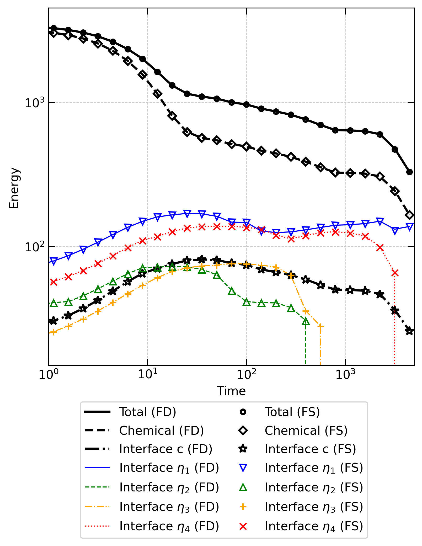
Figure 1: Free energy evolution, for 2D cases, obtained for a $1024^{2}$ grid with FD ($\Delta t=2.225\times 10^{-6}$) and FS ($\Delta t=10^{-3}$) numerical methods.

Figure 2 shows the evolution of the 2D microstructure simulated on a $1024^{2}$ grid using FD ($\Delta t=2.225\times 10^{-6}$), FS ($\Delta t=10^{-3}$), and $\mathcal{O}(\Delta l^{4})$ FS-FD ($\Delta t=10^{-3}$) methods. The $\eta_{1}$, $\eta_{2}$, $\eta_{3}$, and $\eta_{4}$ variants of the phase field (i.e., regions with $\eta_{i}=1$) are represented in blue, green, yellow, and red, respectively, and the concentration field is represented by solid, dashed, and dotted contour lines at values $0.35$, $0.5$, and $0.65$, respectively. In all cases, the microstructure evolves as expected in an Ostwald ripening simulation. Early in the simulation, several particles of each variant exist and interact with one another. Later on, some particles disappear and others of the same variant merge. Finally, after a sufficiently long time, the microstructure reaches steady state with only one $\eta_{1}$ particle remaining. The phase evolution results obtained with the different methods are nearly indistinguishable from each other – thus illustrating that the negligible error levels assessed at $t=100$ in later Section 3.3 can be generalized to the entire duration of the simulation.

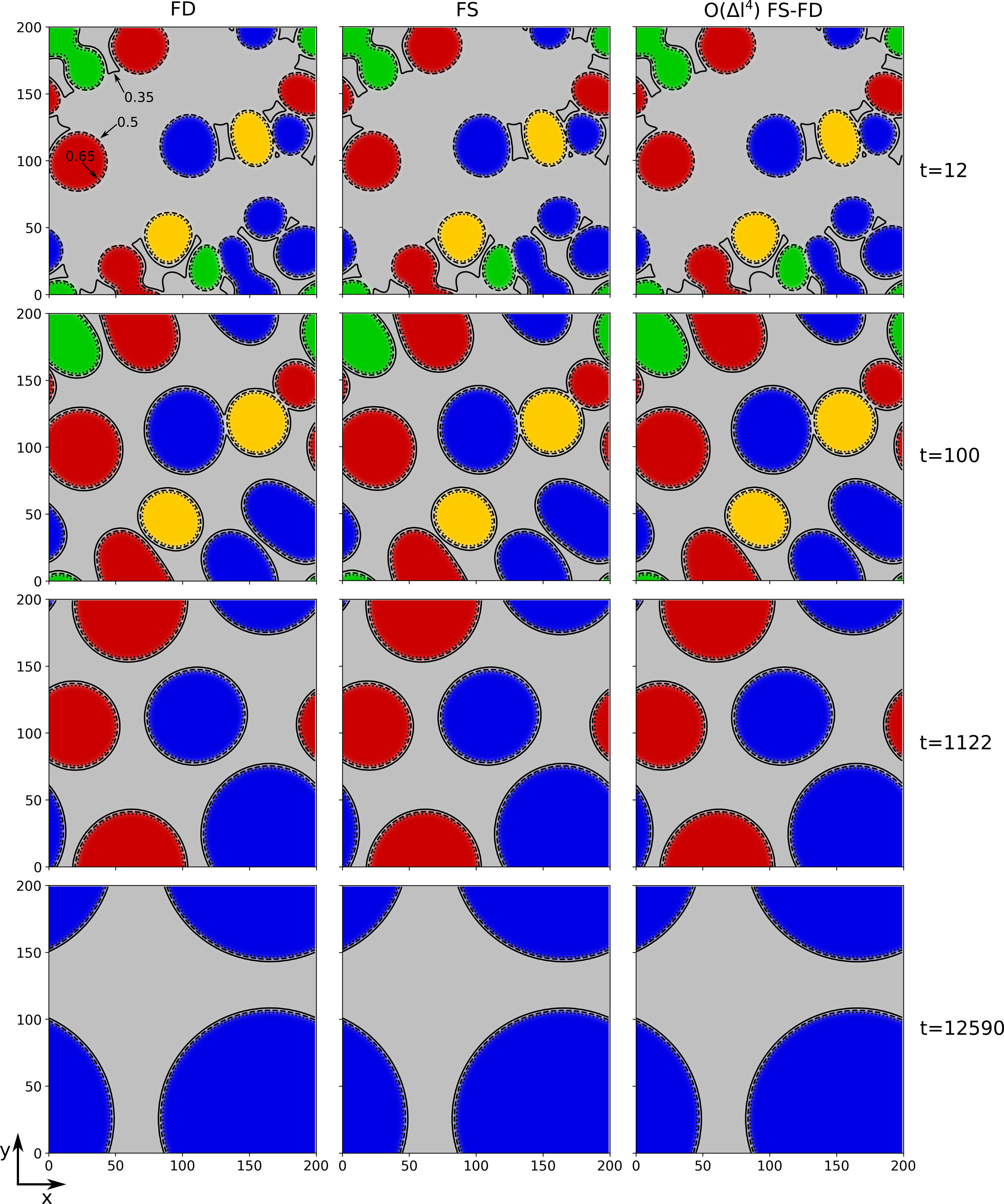
Figure 2: Evolution of phase (color) and concentration (iso-value lines) fields, for 2D cases, at different times (rows) for a grid size of $1024^{2}$ obtained with different methods (columns), namely: (left) FD ($\Delta t=2.225\times 10^{-6}$); (center) FS ($\Delta t=10^{-3}$), and (right) $\mathcal{O}(\Delta l^{4})$ FS-FD ($\Delta t=10^{-3}$).

Figure 3 shows the evolution of the 3D microstructure simulated on a $256^{3}$ grid using the FS method. As in Fig. 2, the $(\eta_{i}=0.5)$ interfaces for $i=1$, 2, 3, and 4 are represented in blue, green, yellow, and red, respectively. Isovalues of the concentration field along the central $(z=l_{z}/2)$ plane are represented from $c=0.3$ to $c=0.8$ with steps of 0.05. In all cases, the microstructure evolves as expected in an Ostwald ripening simulation. Several small particles of each variant exist at early times and one big (here, planar) particle of $\eta_{1}$ remains when the microstructure reaches steady state. The microstructure evolves faster in the 3D cases because the domain size and particles are relatively smaller than in 2D cases.

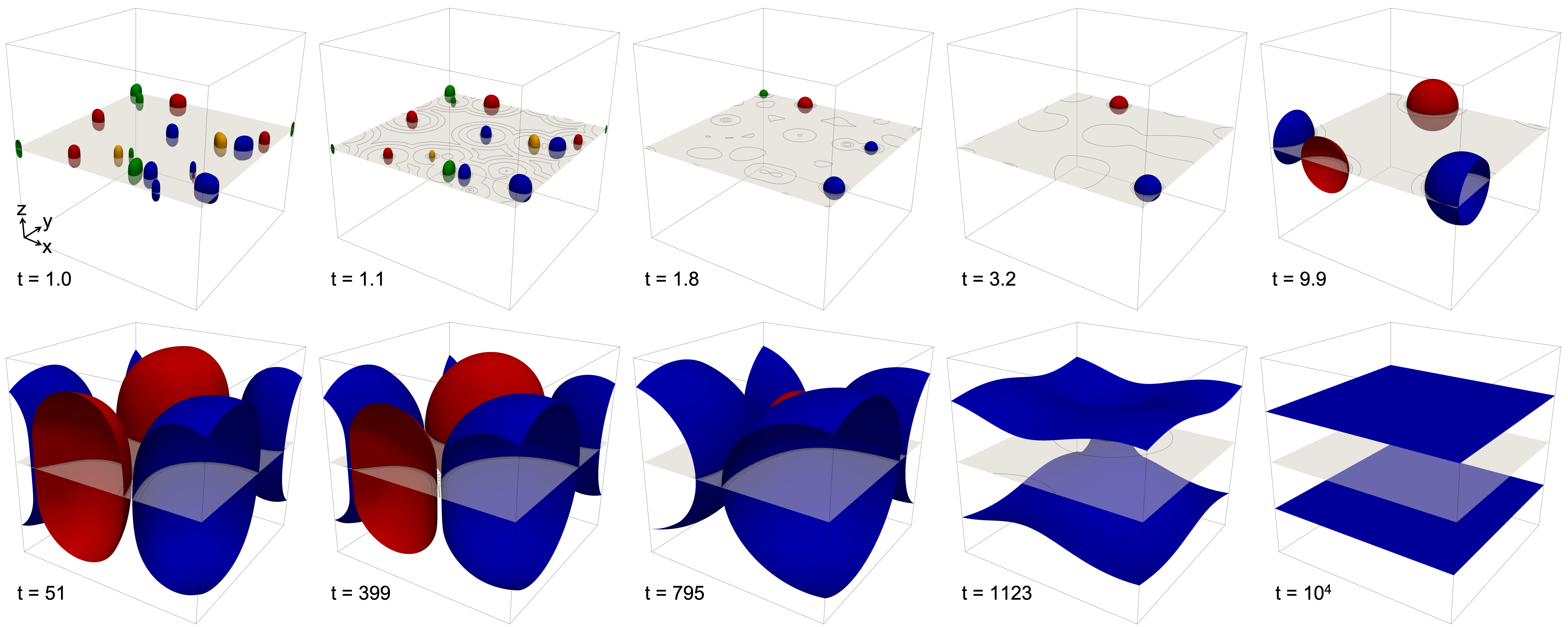
Figure 3: Evolution of $(\eta_{i}=0)$ interfaces (color) and concentration (isovalue lines along the $(z=l_{z}/2)$ plane) fields, for a 3D simulation with $n=256^{3}$ obtained with FS method.

3.2 Computational performance

The wall clock time required to complete the 2D simulations from time $1$ to $100$ (dimensionless) is presented in Figure 4.a. For each studied case, 6 simulations are run with the same parameters and the wall clock time is determined by averaging the results because a variation in the wall clock time consumed by Scikit-CUDA is observed. Different line thicknesses or symbol sizes represent different $\Delta t$ (thicker/bigger: lower $\Delta t$). Solid blue lines show the FS algorithm, symbols show the FS-FD algorithm with $\mathcal{O}(\Delta l^{2})$ (yellow $\circ$) or $\mathcal{O}(\Delta l^{4})$ (green $\times$), and dashed red lines show the corresponding FD algorithm. As expected, the wall clock time decreases with $\Delta t$ due to the fact that fewer steps are necessary to reach $t=100$. For a given $\Delta t$, the performance of all FS methods is similar because $\|\boldsymbol{\xi}\|^{2}$ is computed only once at the initialization stage.

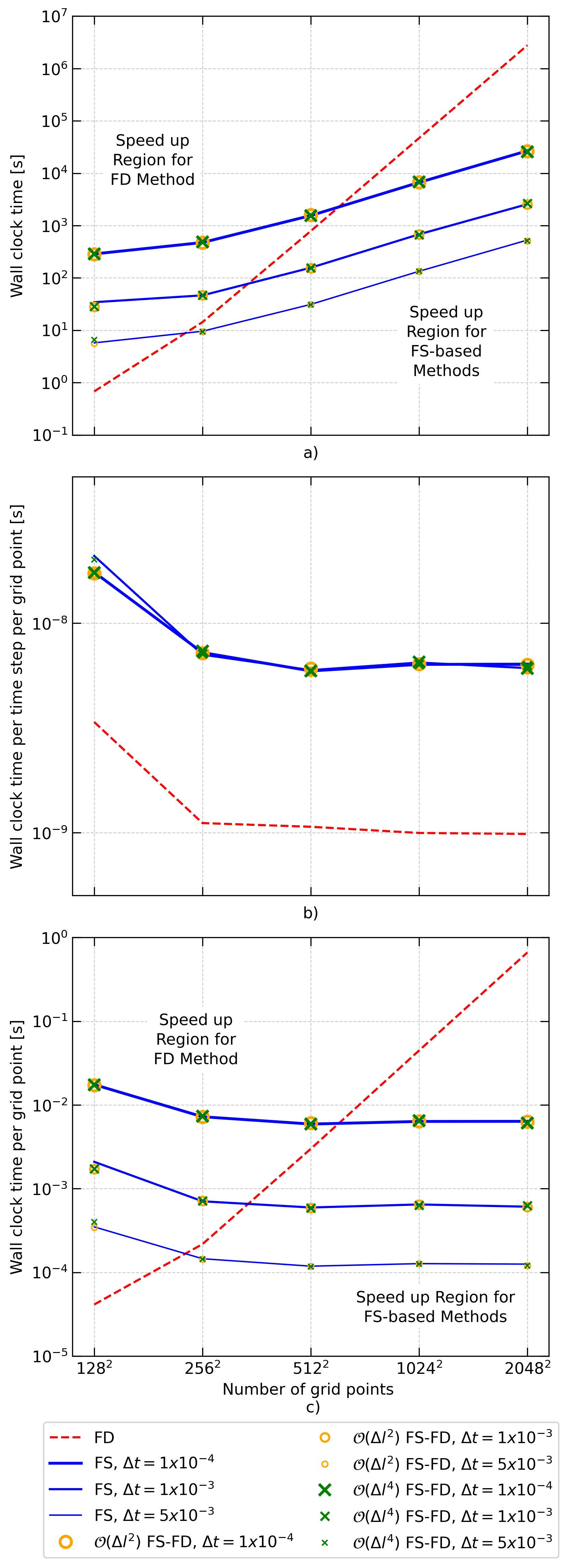
Figure 4: Computational performance for 2D cases. a) wall clock time, b) wall clock time per time step per grid point, and c) wall clock time per grid point, all of them for different numbers of grid points.

The wall clock time to compute one time step per grid point is shown in Figure 4.b for 2D simulations. This metric is independent of the FS method and the chosen time step. For all methods, it is significantly higher for $n=128^{2}$, which is attributed to parallelization inefficiency when the grid size is small. Indeed, a $128^{2}$ domain corresponds to less than 3.8 grid points per CUDA core, which is not optimal in the absence of any load balancing supervision. The required solution time per grid point per time step using the FS methods is between 5.2 and 6.5 times higher than using the FD method. This is due to the required computation, at every step, of $\mathcal{F}$ of the partial derivatives of $f_{chem}$ at time $t$, and $\mathcal{F}^{-1}$ of $\widehat{c}$ and $\widehat{\eta_{i}}$ at time $t+\Delta t$, which are not required in FD. Hence, FS methods perform best when $\Delta t$ is sufficiently larger than with the FD method, namely by a factor of 6.5 or more, in order to compensate for the extra time needed to calculate $\mathcal{F}$ and $\mathcal{F}^{-1}$. This compensation is observed at $n\geq 256^{2}$ for $\Delta t=5\times 10^{-3}$ (i.e., $\Delta t_{\rm FS}/\Delta t_{\rm FD}=9.8$), at $n\geq 512^{2}$ for $\Delta t=10^{-3}$ (i.e., $\Delta t_{\rm FS}/\Delta t_{\rm FD}=28.1$), and at $n\geq 1024^{2}$ for $\Delta t=10^{-4}$ (i.e., $\Delta t_{\rm FS}/\Delta t_{\rm FD}=44.9$), as seen in Figures 4.a and 4.c. When $n=128^{2}$, the FD method has a better performance in comparison with the FS ones, but its accuracy is not as good, as discussed in Section 3.3.

The wall clock time required to complete the 3D simulations from time $1$ to $100$ (dimensionless) is presented in Figure 5.a. Solid blue lines show the FS algorithm, dashed yellow lines show the FS-FD algorithm with $\mathcal{O}(\Delta l^{2})$, dashed green lines show the FS-FD algorithm with $\mathcal{O}(\Delta l^{4})$, and dashed red lines show the corresponding FD algorithm. For each case with $n=128{3}$ and $n=256^{3}$, computed with FS-based methods, the wall clock time is determined by averaging the results obtained from 6 simulations because the wall clock time consumed by Scikit-CUDA presents some variations. The same behavior as in 2D cases is observed and the performance is in favor of FS methods when $\Delta t$ is sufficiently larger than with the FD method, by a factor of 4.3 or more, in order to compensate for the extra time needed to calculate $\mathcal{F}$ and $\mathcal{F}^{-1}$. This compensation is observed at $n\geq 128^{3}$ ($\Delta t_{\rm FS}/\Delta t_{\rm FD}=62.9$). When $n<128^{3}$, the FD method has a better performance in comparison with the FS ones, but its accuracy is not as good. The wall clock time to compute one step per each grid point is shown in Figure 5.b. This metric is independent of the FS method and the chosen time step. In all cases, it increases significantly for $n=16^{3}$ and $n=32^{3}$, which is related to parallelization inefficiency when the grid size is small. The required solution time per time step per grid point using the FS methods is between 2.3 and 4.3 times higher than the using the FD method. This ratio is lower than in 2D cases because FS methods compute $\|\boldsymbol{\xi}\|^{2}$ at the begining of the simulation and in this way the number of operations per grid point is the same for 2D and 3D, but it is not the case for FD method, which uses 5-point stencil in 2D and 7-point stencil in 3D, increasing the computational cost per grid point, as illustrated in Figure 5.b with 2D cases shown as symbols.

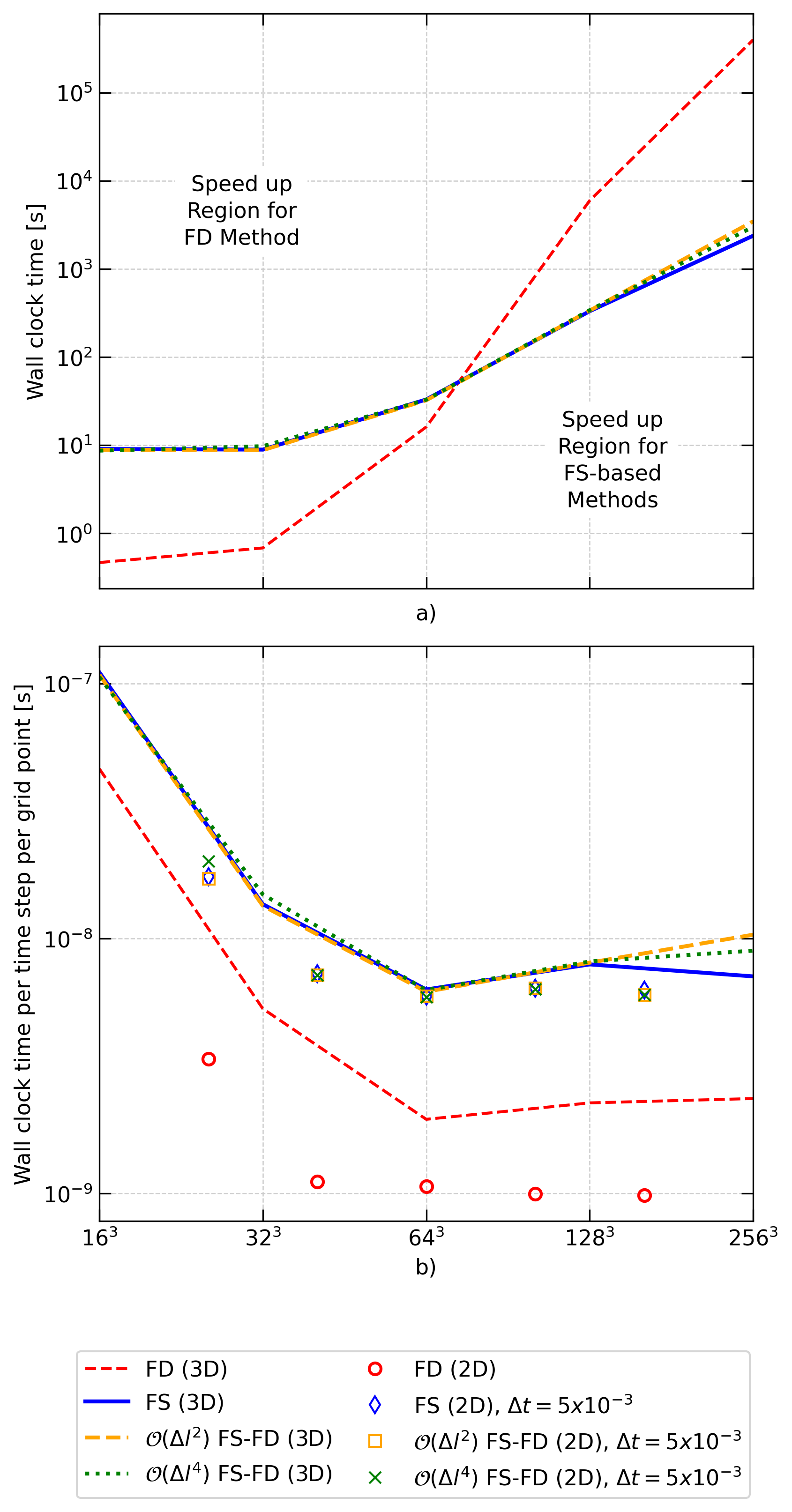
Figure 5: Computational performance for 3D cases for different numbers of grid points (see Table 2): a) wall clock time and b) wall clock time per time step per grid point.

Regarding GPU memory (RAM) consumption, the FS and FD 2D simulations with $n=2048^{2}$ require 1.93 GB and 0.46 GB, respectively, and the FS and FD 3D simulations with $n=256^{3}$ require 7.14 GB and 1.52 GB, respectively. This difference arises from the fact that 12 complex arrays are needed for the FS scheme compared to the 6 real ones for FD. The increase in performance (and accuracy, as shown in Section 3.3) provided by FS methods thus comes at the cost of a higher memory consumption – but even the 7 GB required by the largest $256^{3}$ cases with 5 tracked fields easily fits within almost modern GPU.

3.3 Accuracy of the results

The accuracy of results obtained for different values of $\Delta t$ and $n$ is quantified, in comparison to a reference solution by measuring the L₂ normalized global error of a field $\phi$ computed at $t=100$ as:

$$E_{\phi}=\dfrac{\int_{V}(\phi_{0}-\phi)^{2}\,dV}{\int_{V}\phi_{0}^{2}\,dV}$$ (22)

where $\phi_{0}$ is the reference solution field and $\phi$ is the assessed solution field for a given test condition.

In the absence of a reference (e.g., analytical) solution, the reference solution for 2D simulations is chosen as the FS implementation with the lowest $\Delta t=10^{-4}$ and the highest $n=2048^{2}$. For the phase fields, the solution of $\eta_{i}$ ($i=1\text{ to }4$) are added together into a field $\eta$. We only compare accuracy for the 2D calculations, as we consider that the finest $256^{3}$ grid is not fine enough to be considered a reference, and we observed trends observed in 2D to be generalizable to 3D.

Figure 6 shows the errors, in percentage, for (a) concentration and (b) phase fields with different numbers of grid points and time step size for 2D cases. As expected, the errors decrease with increasing number of grid points and decreasing $\Delta t$. For the coarsest $n=128^{2}$ grid, good accuracy (i.e., an error lower than 1%) is achieved, except for FD and $\mathcal{O}(\Delta l^{2})$ FS-FD methods, giving errors of $E_{c}[\%]=2.03$ and $E_{\eta}[\%]=7.74$. FS and $\mathcal{O}(\Delta l^{4})$ FS-FD methods provide more accurate results than FD or $\mathcal{O}(\Delta l^{2})$ FS-FD because they lead to more accurate spatial derivatives even on coarser grids. Comparing two cases with equivalent errors, namely $E_{c}[\%]\approx 10^{-6}$ and $E_{\eta}[\%]\approx 2\times 10^{-5}$, the wall clock time ratio between FS ($n=256^{2}$ and $\Delta t=10^{-3}$) and FD ($n=2048^{2}$ and $\Delta t=1.490\times 10^{-7}$) is over four orders of magnitude ($6\times 10^{4}$), at 46 seconds and 32 days, respectively. Using the $\mathcal{O}(\Delta l^{4})$ FS-FD algorithm, a lower time step $\Delta t=10^{-4}$ is required to achieve a similar accuracy. Since the required time step is one order of magnitude lower than with FS, the resulting speed-up compared to FD at a similar error is one order of magnitude lower ($\mathcal{O}(\Delta l^{4})$ FS-FD is still faster than FD by over three orders of magnitude).

In summary, for simulations requiring a sufficient level of accuracy, the FS method, and to a less extent the $\mathcal{O}(\Delta l^{4})$ FS-FD method, are significantly more efficient than the classical FD algorithm, due to less stringent requirements on both spatial and temporal discretization.

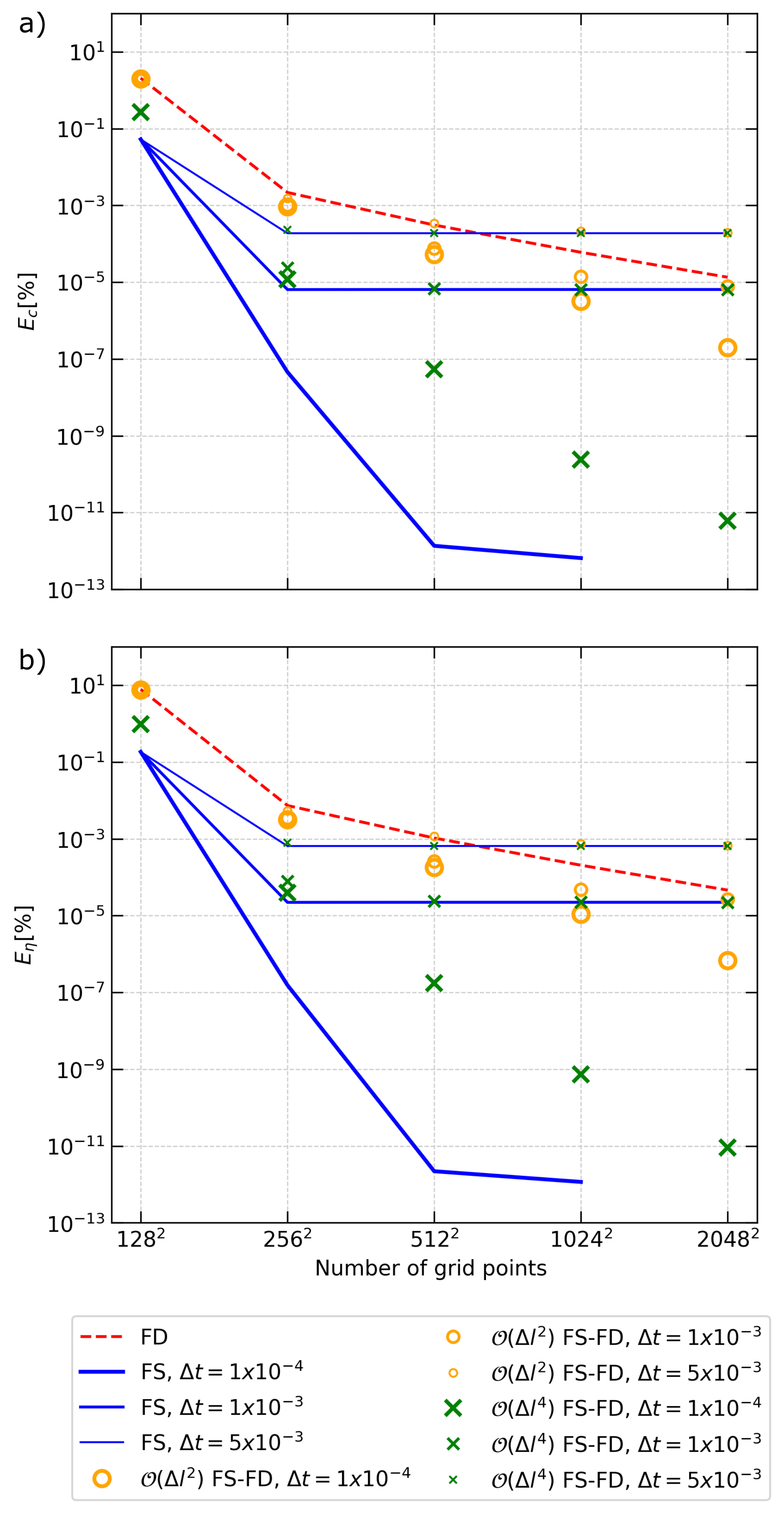
Figure 6: Error for 2D cases of a) concentration field and b) phase field for different numbers of grid point.

4 Conclusions

Here, we compared different numerical resolution methods for a benchmark Ostwald-ripening phase-field benchmark simulation. Our spectral solver makes use of a semi-implicit Fourier spectral-based numerical method, implemented in Python language, and parallelized on a single GPU. By comparison with first-order forward Euler finite difference for time discretization and second-order centered finite difference for space discretization, also parallelized on a single GPU, we conclude that:

• Fourier spectral-based methods significantly outperform finite differences when a large number of spatial grid points is required. This advantage is due to the much larger stable time step afforded by semi-implicit FS methods against explicit FD, in spite of the additional operations (transformation and anti-transformation of complex/scalar variables) per time step required by the FS solver. For our implementation, the performance is in favor of FS methods as long as $\Delta t$ is larger than the maximum stable time step for the FD method by a factor of 6.5 in 2D or 4.3 in 3D.

• The time step stability does not strongly depend on the grid size in the semi-implicit FS-based methods, which represents a significant advantage when a fine spatial discretization is required.

• Under the same temporal and spatial discretization conditions, all of the Fourier spectral-based methods (namely FS or FS-FD) have the same computational performance, but the highest accuracy is obtained with the Fourier spectral scheme.

• For a similar level of accuracy (i.e., of error) for both phase and concentration fields, the computational performance of the FS and FS-FD $\mathcal{O}(\Delta l^{4})$ methods exceeds that of explicit FD by more than four orders of magnitude.

• The Python programming allowed an easy implementation of the model and exploitation of the benefit of GPU device through the CUDA kernel implementation.

• For the consider benchmark, Fourier spectral-based methods required 4.7 times more memory (RAM) than the explicit FD, which may limit the applicability of the former for 3D domains with fine grids using single-GPU hardware.

Data Availability

Data will be made available on request.

References

- [1] L.-Q. Chen, “Phase-field models for microstructure evolution,” Annual Review of Materials Research, vol. 32, no. 1, pp. 113–140, 2002.
- [2] W. J. Boettinger, J. A. Warren, C. Beckermann, and A. Karma, “Phase-field simulation of solidification,” Annual Review of Materials Research, vol. 32, no. 1, pp. 163–194, 2002.
- [3] N. Moelans, B. Blanpain, and P. Wollants, “An introduction to phase-field modeling of microstructure evolution,” Calphad, vol. 32, no. 2, pp. 268–294, 2008.
- [4] I. Steinbach, “Phase-field models in materials science,” Modelling and Simulation in Materials Science and Engineering, vol. 17, no. 7, p. 073001, 2009.
- [5] M. R. Tonks and L. K. Aagesen, “The phase field method: mesoscale simulation aiding material discovery,” Annual Review of Materials Research, vol. 49, pp. 79–102, 2019.
- [6] D. Tourret, H. Liu, and J. LLorca, “Phase-field modeling of microstructure evolution: Recent applications, perspectives and challenges,” Progress in Materials Science, vol. 123, p. 100810, 2022. A Festschrift in Honor of Brian Cantor.
- [7] W. L. George and J. A. Warren, “A parallel 3d dendritic growth simulator using the phase-field method,” Journal of Computational Physics, vol. 177, no. 2, pp. 264–283, 2002.
- [8] B. Nestler, “A 3D parallel simulator for crystal growth and solidification in complex alloy systems,” Journal of Crystal Growth, vol. 275, no. 1, pp. e273–e278, 2005. Proceedings of the 14th International Conference on Crystal Growth and the 12th International Conference on Vapor Growth and Epitaxy.
- [9] A. Vondrous, M. Selzer, J. Hötzer, and B. Nestler, “Parallel computing for phase-field models,” The International Journal of High Performance Computing Applications, vol. 28, no. 1, pp. 61–72, 2014.
- [10] N. Provatas, N. Goldenfeld, and J. Dantzig, “Adaptive mesh refinement computation of solidification microstructures using dynamic data structures,” Journal of Computational Physics, vol. 148, no. 1, pp. 265–290, 1999.
- [11] M. Greenwood, K. Shampur, N. Ofori-Opoku, T. Pinomaa, L. Wang, S. Gurevich, and N. Provatas, “Quantitative 3D phase field modelling of solidification using next-generation adaptive mesh refinement,” Computational Materials Science, vol. 142, pp. 153–171, 2018.
- [12] J. Rosam, P. K. Jimack, and A. Mullis, “An adaptive, fully implicit multigrid phase-field model for the quantitative simulation of non-isothermal binary alloy solidification,” Acta Materialia, vol. 56, no. 17, pp. 4559–4569, 2008.
- [13] P. Bollada, C. Goodyer, P. Jimack, A. Mullis, and F. Yang, “Three dimensional thermal-solute phase field simulation of binary alloy solidification,” Journal of Computational Physics, vol. 287, pp. 130–150, 2015.
- [14] A. Yamanaka, T. Aoki, S. Ogawa, and T. Takaki, “GPU-accelerated phase-field simulation of dendritic solidification in a binary alloy,” Journal of Crystal Growth, vol. 318, no. 1, pp. 40–45, 2011. The 16th International Conference on Crystal Growth (ICCG16)/The 14th International Conference on Vapor Growth and Epitaxy (ICVGE14).
- [15] S. Sakane, T. Takaki, M. Ohno, T. Shimokawabe, and T. Aoki, “GPU-accelerated 3D phase-field simulations of dendrite competitive growth during directional solidification of binary alloy,” IOP Conference Series: Materials Science and Engineering, vol. 84, p. 012063, jun 2015.
- [16] T. Shimokawabe, T. Aoki, T. Takaki, T. Endo, A. Yamanaka, N. Maruyama, A. Nukada, and S. Matsuoka, “Peta-scale phase-field simulation for dendritic solidification on the TSUBAME 2.0 supercomputer,” in Proceedings of 2011 International Conference for High Performance Computing, Networking, Storage and Analysis, SC ’11, (New York, NY, USA), Association for Computing Machinery, 2011.
- [17] S. Sakane, T. Takaki, and T. Aoki, “Parallel-GPU-accelerated adaptive mesh refinement for three-dimensional phase-field simulation of dendritic growth during solidification of binary alloy,” Materials Theory, vol. 6, no. 1, p. 3, 2022.
- [18] T. Takaki, S. Sakane, M. Ohno, Y. Shibuta, T. Aoki, and C.-A. Gandin, “Competitive grain growth during directional solidification of a polycrystalline binary alloy: Three-dimensional large-scale phase-field study,” Materialia, vol. 1, pp. 104–113, 2018.
- [19] Y. Song, F. L. Mota, D. Tourret, K. Ji, B. Billia, R. Trivedi, N. Bergeon, and A. Karma, “Cell invasion during competitive growth of polycrystalline solidification patterns,” Nature Communications, vol. 14, no. 1, p. 2244, 2023.
- [20] J. Hötzer, M. Jainta, P. Steinmetz, B. Nestler, A. Dennstedt, A. Genau, M. Bauer, H. Köstler, and U. Rüde, “Large scale phase-field simulations of directional ternary eutectic solidification,” Acta Materialia, vol. 93, pp. 194–204, 2015.
- [21] S. Lucarini, M. V. Upadhyay, and J. Segurado, “FFT based approaches in micromechanics: fundamentals, methods and applications,” Modelling and Simulation in Materials Science and Engineering, vol. 30, no. 2, p. 023002, 2021.
- [22] L. Chen and J. Shen, “Applications of semi-implicit Fourier-spectral method to phase field equations,” Computer Physics Communications, vol. 108, no. 2, pp. 147–158, 1998.
- [23] J. Zhu, L.-Q. Chen, J. Shen, and V. Tikare, “Coarsening kinetics from a variable-mobility cahn-hilliard equation: Application of a semi-implicit fourier spectral method,” Physical Review E, vol. 60, no. 4, p. 3564, 1999.
- [24] W. Feng, P. Yu, S. Hu, Z. Liu, Q. Du, and L. Chen, “Spectral implementation of an adaptive moving mesh method for phase-field equations,” Journal of Computational Physics, vol. 220, no. 1, pp. 498–510, 2006.
- [25] L. Chen, J. Chen, R. Lebensohn, Y. Ji, T. Heo, S. Bhattacharyya, K. Chang, S. Mathaudhu, Z. Liu, and L.-Q. Chen, “An integrated fast fourier transform-based phase-field and crystal plasticity approach to model recrystallization of three dimensional polycrystals,” Computer Methods in Applied Mechanics and Engineering, vol. 285, pp. 829–848, 2015.
- [26] M. Cheng and J. A. Warren, “An efficient algorithm for solving the phase field crystal model,” Journal of Computational Physics, vol. 227, no. 12, pp. 6241–6248, 2008.
- [27] G. Tegze, G. Bansel, G. I. Tóth, T. Pusztai, Z. Fan, and L. Gránásy, “Advanced operator splitting-based semi-implicit spectral method to solve the binary phase-field crystal equations with variable coefficients,” Journal of Computational Physics, vol. 228, no. 5, pp. 1612–1623, 2009.
- [28] X. Shi, H. Huang, G. Cao, and X. Ma, “Accelerating large-scale phase-field simulations with GPU,” AIP Advances, vol. 7, no. 10, p. 105216, 2017.
- [29] J. Lee and K. Chang, “Effect of magnetic ordering on the spinodal decomposition of the Fe-Cr system: A GPU-accelerated phase-field study,” Computational Materials Science, vol. 169, p. 109088, 2019.
- [30] A. Eghtesad, K. Germaschewski, I. J. Beyerlein, A. Hunter, and M. Knezevic, “Graphics processing unit accelerated phase field dislocation dynamics: Application to bi-metallic interfaces,” Advances in Engineering Software, vol. 115, pp. 248–267, 2018.
- [31] A. Jokisaari, P. Voorhees, J. Guyer, J. Warren, and O. Heinonen, “Benchmark problems for numerical implementations of phase field models,” Computational Materials Science, vol. 126, pp. 139–151, 2017.
- [32] A. A. Wheeler, W. J. Boettinger, and G. B. McFadden, “Phase-field model for isothermal phase transitions in binary alloys,” Physical Review A, vol. 45, no. 10, p. 7424, 1992.
- [33] J. Zhu, T. Wang, A. Ardell, S. Zhou, Z. Liu, and L. Chen, “Three-dimensional phase-field simulations of coarsening kinetics of particles in binary ni–al alloys,” Acta Materialia, vol. 52, no. 9, pp. 2837–2845, 2004.
- [34] J. W. Cahn, “On spinodal decomposition,” Acta Metallurgica, vol. 9, no. 9, pp. 795–801, 1961.
- [35] S. M. Allen and J. W. Cahn, “A microscopic theory for antiphase boundary motion and its application to antiphase domain coarsening,” Acta Metallurgica, vol. 27, no. 6, pp. 1085–1095, 1979.
- [36] W. H. Müller, “Mathematical vs. experimental stress analysis of inhomogeneities in solids,” Journal De Physique Iv, vol. 06, 1996.
- [37] L. Givon, “Scikit-CUDA Documentation,” https://scikit-cuda.readthedocs.io/en/latest, 2021.
- [38] A. Klöckner, N. Pinto, Y. Lee, B. Catanzaro, P. Ivanov, and A. Fasih, “PyCUDA and PyOpenCL: A Scripting-Based Approach to GPU Run-Time Code Generation,” Parallel Computing, vol. 38, no. 3, pp. 157–174, 2012.