Bifurcations of Riemann Ellipsoids

Abstract

We give an account of the various changes in the stability character in the five types of Riemann ellipsoids by establishing the occurrence of different quasi-periodic Hamiltonian bifurcations. Suitable symplectic changes of coordinates, that is, linear and non-linear normal form transformations are performed, leading to the characterisation of the bifurcations responsible of the stability changes. Specifically we find three types of bifurcations, namely, Hamiltonian pitchfork, saddle-centre and Hamiltonian-Hopf in the four-degree-of-freedom Hamiltonian system resulting after reducing out the symmetries of the problem. The approach is mainly analytical up to a point where non-degeneracy conditions have to be checked numerically. We also deal with the regimes in the parametric plane where Liapunov stability of the ellipsoids is accomplished. This strong stability behaviour occurs only in two of the five types of ellipsoids, at least deductible only from a linear analysis.

MSC Classification]70H14, 37J20

1 Introduction

One of the relevant problems Newton addresses in his Principia Principia is the determination of the shape of the Earth when rotating around its axis. He assumes the Earth to be a homogeneous axisymmetric self-gravitating fluid slowly rotating around its axis and shows that rotation makes the body oblate. This investigation constitutes the first attempt at determining how rotation affects the shape of a body whose surface is not rigid and is the beginning of a fruitful line of research that notable scientists, such as MacLaurin or Jacobi follow. The models addressed by these authors assume that the fluid is stationary in a frame rotating with the body.

In 1860, Dirichlet Dirichlet starts a new line of research when considering non-rigid movements. He contemplates configurations whose motion in an inertial frame is a linear function of the coordinates. In particular, he considers

$$x(t,y)=F(t)\,y,\qquad F(t)\in SL(3),$$ (1)

where $x(t,y)$ is the position of a particle at time $t$ in a fixed reference system, $y$ are the coordinates of the particle in the reference system centred at the body and $SL(3)$ denotes the special linear group of degree $3$ over ${\mathbb{R}}$. Dirichlet addresses the problem of determining the conditions for these configurations to have an ellipsoidal figure at any moment Dirichlet; chandrasekhar1969ellipsoidal; fasso2001stability. Assuming that the reference configuration of the fluid mass is a radius $\ignorespaces\rho$ -ball, the free surface of the fluid mass determined by (1) is an ellipsoid with semi-axes $\ignorespaces\rho a_{1},\rho a_{2},\rho a_{3}$ , where $\ignorespaces a_{i}$ are the singular values of matrix $\ignorespaces F$ , i.e. the square root of the eigenvalues of $FF^{T}$ or $F^{T}F$.

It is Euler’s equations that govern the dynamics of adiabatic and inviscid flows. They are a set of quasi-linear partial differential equations that correspond to the Navier-Stokes equations with no viscosity and no thermal conductivity. Dirichlet’s philosophy is using Lagrangian formulation to reduce Euler’s equations to a system of ordinary differential equations such that the position of the particle in the ellipsoid at any time is a linear homogeneous function of its initial position. He proves that (1) forms an invariant subsystem of Euler’s equations of fluid dynamics. It is his student, Dedekind, who publishes Dirichlet’s work posthumously and completes some results.

Riemann Riemann subsequently continues Dirichlet’s work and reformulates the equations of motion (1) in a convenient way to study steady asymmetric configurations. Riemann determines and classifies all possible relative equilibrium conditions and analyses the stability of the corresponding equilibria. They are characterised by different relations among the angular velocities and the figures’ semi-axes. There are five kinds of these states called Riemann ellipsoids. They are denoted by $S_{2}$, $S_{3}$, I, II, III and are motions of the type (1) such that

$$F(t)=\exp(t\,\Omega_{l})\,A\exp(-t\,\Omega_{r}),$$ (2)

where

$$A=\mbox{diag}\left(a_{1},a_{2},a_{3}\right),\,\Omega_{l},\Omega_{r}\,\,\mbox{being constant antisymmetric $(3\times 3)$-matrices.}$$

The equilibrium form does not perform a rigid motion, since it is a composition of an internal rotation together with a stretch along the principal axes and a spatial rotation such that the free surface retains a rotating ellipsoidal shape. Thence, Riemann ellipsoids are steady states of an ideal incompressible homogeneous self-gravitating fluid mass that has an ellipsoidal shape. The fluid particles describe either periodic or quasi-periodic rosette-shaped motions. In this latter case they depend on the two angular frequencies, $\omega_{l}$ and $\omega_{r}$, respectively associated to matrices $\Omega_{l}$ and $\Omega_{r}$. For ellipsoids $S_{2}$ and $S_{3}$ vectors $\omega_{l}$ and $\omega_{r}$ are parallel to the same principal axis of the ellipsoid; this axis is either the shortest for $S_{3}$ or the middle one for $S_{2}$. For ellipsoids I, II and III, both $\omega_{l}$ and $\omega_{r}$ lie in one of the two principal planes containing the longest ellipsoid’s principal axis. Given an $S$-type Riemann ellipsoid we say it is co-parallel when the dot product of $\omega_{l}$ and $\omega_{r}$ is positive, otherwise we call it counter-parallel. All $S_{3}$-ellipsoids are counter-parallel, while the $S_{2}$-ellipsoids may be co-parallel or counter-parallel.

Ensuing contributions by Liapunov, Poincaré and Cartan enhance knowledge of this problem. Chandrasekhar chandrasekhar1965; chandrasekhar1966; chandrasekhar1969ellipsoidal enlarges and completes the work initiated by the previous authors, studying the linear (its spectral version) stability of the ellipsoids by making use of the Virial Theorem of Mechanics. In particular, he presents in a unified way Dirichlet and Dedekind’s approaches, MacLaurin spheroids, Jacobi and Dedekind ellipsoid and Riemann ellipsoids. In lebovitz1996, Lebovitz explains why some of Riemann’s conclusions on stability are incorrect, in contrast to Chandrasekhar’s. Rosensteel Rosensteel1; Rosensteel2; Rosensteel3 reformulates the problem from a symplectic geometry point of view and also adapts it to nuclear physics models. Moreover, applying symplectic geometry Lewis Lewis gives an account of the stability of MacLaurin spheroids, already accomplished by Riemann and Chandrasekhar. Paper roberts1999symmetries continues with the Hamiltonian geometric approach to Riemann’s classification of equilibrium ellipsoids. Related amendments to Riemann’s conclusions are included in Marshalek. The Hamiltonian formulation is also discussed in MoLeBi. A recent differential geometric approach can be seen in OlmosSousa, where the authors deal with the non-linear stability of some particular Riemann ellipsoids that can be formulated as three-degree-of-freedom Hamiltonian systems. Indeed, there is a wide bibliography on the theme. For a historical account see, for instance chandrasekhar1969ellipsoidal. A good review paper with some new results on the dynamics of self-gravitating liquid and gas ellipsoids is BorisovKilinMamaev.

In fasso2001stability; fasso2014erratum Fassò and Lewis perform a thorough analysis of the stability of Riemann ellipsoids, improving and completing previous studies appearing in the literature, in particular, they amend some of Chandrasekhar’s findings. Especially, they notice that the regions of known instability of the ellipsoids of types II and III are substantially smaller than those sought by Chandrasekhar. As a first step, Fassò and Lewis perform a linear (the so-called spectral) stability analysis, as they focus on the eigenvalues of the linearisation matrix. In a second step they deal with the non-linear stability of the ellipsoids, applying Nekhoroshev theory on exponentially long-time stability of solutions. The approach followed by Fassò and Lewis can be interpreted as semi-numerical: when possible, the calculations are carried out symbolically, but the determination of the bifurcation curves is done numerically. In this paper we continue their work and deepen the analysis of the dynamics and stability of Riemann ellipsoids. Our notations and calculations are based in theirs. We have reproduced the material from fasso2001stability needed for the understanding of the present manuscript.

We present a systematic study of the bifurcations arising for Riemann ellipsoids. This problem is far from trivial, as the computations we perform imply manipulating large formulae. The Hamiltonian function accounts for a system of four degrees of freedom and it depends on an incomplete elliptic integral that is handled in closed form, that is, without resorting to numerical approximations. Our study is mostly analytical, said in other words, in closed form: the linear and non-linear normal forms and related transformations are all analytical, but some final checks proving non-degeneracy (normally that an expression does not vanish on a bifurcation line) should be made numerically, as we shall mention adequately. Moreover, all calculations have been carried out with Mathematica, using integer arithmetic. Notice that the numerical testing does not reduce the rigour of our analysis, and we can state the occurrence of different bifurcations by means of theorems. Regarding previous approaches dealing with bifurcations analysis for the four-degree-of-freedom Riemann ellipsoids we only know of a recent reference benavides, which is mainly numerical. On our side we prove that there are up to three types of quasi-periodic bifurcations, the most abundant being the Hamiltonian-Hopf bifurcations, that arise for the ellipsoids of types I, II and III. However, the ellipsoids $S_{2}$ experience a Hamiltonian-pitchfork bifurcation, whereas type II-ellipsoids undergo a saddle-centre bifurcation. All these bifurcations take place in the parametric plane determined by the two essential parameters, the same plane as the one considered in chandrasekhar1969ellipsoidal and fasso2001stability.

Quasi-periodic bifurcations occurring in the Hamiltonian context have been extensively studied by Broer, Hanßman and co-workers, and we follow the monograph hanssmann2006local to establish our results on the bifurcations of Riemann ellipsoids.

In future we will provide the non-linear stability analysis of the different Riemann ellipsoids. By this we mean stability of formal type, the so-called Lie stability, which in particular generalises Nekhoroshev-type stability for equilibrium points of elliptic character, see Carcamo2021.

The paper is structured as follows. Section 2 presents the Hamiltonian formulation of the system. Section 3 provides the equilibria of the problem and their regions of existence. The analysis of the bifurcations can be found in the subsequent sections. The stability of $S_{2}$-ellipsoids is dealt with in Section 4. The main finding concerning these ellipsoids is a Hamiltonian pitchfork bifurcation, which is studied through a non-linear approach. Ellipsoids of type $S_{3}$ are Liapunov stable, as shown in Section 5. This result is due to Riemann, we simply recover it for completeness. In Section 6 we deal with type-I ellipsoids, analysing the particular case of irrotational ellipsoids (one of the two angular frequencies vanishes and the Hamiltonian system can be reduced by one degree of freedom). Concretely we study its stability and make the observation that the transition from stability to instability is done by means of two Hamiltonian-Hopf bifurcation points. There is a saddle-centre bifurcation related to type-II ellipsoids that is described in Section 7. For type-III ellipsoids there is a Hamiltonian-Hopf bifurcation that is explained in Section LABEL:TypeIII. Finally, there is a global bifurcation involving the $S_{2}$ and type-III ellipsoids that is described in Section LABEL:global. This bifurcation corresponds to a global viewpoint of the pitchfork bifurcation tackled in Section 4. The main achievements and some remarks regarding possible future approaches are outlined in Section LABEL:conclusions. Appendix LABEL:C1C2 provides explicit expressions of two improper integrals in terms of two incomplete elliptic integrals that are required in our approach. In Appendix LABEL:CoefficientsL we place the essential formulae related to the regime of the $S_{2}$-ellipsoids where the pitchfork bifurcation arises. Finally, Appendix LABEL:Linearization is devoted to the description of Markeev’s procedure to compute the linear normal form of a Hamiltonian system corresponding to an elliptic equilibrium. We also collect the entries of the transformation matrix used to deal with the pitchfork bifurcation analysis.

The calculations presented in Appendix LABEL:C1C2 are crucial for the achievements obtained on the Riemann ellipsoids. Actually, the determination of these two functions allows us to explicitly write the coordinates of all ellipsoids, as well as the sets in the parametric plane where the ellipsoids are properly defined. Moreover, excepting the curves associated to Hamiltonian-Hopf bifurcations that, much as determined analytically, are approximated by applying numerical techniques, making the approach practical, the rest of lines and points in the parametric plane corresponding to changes in stability have been obtained in closed form. This is in part due to the improper integrals provided in Appendix LABEL:C1C2. We shall give details on this feature when dealing with the study performed in the five ellipsoids.

Our analysis has not pursued the heavy task of seeking all stability regions and bifurcation curves in the parametric plane (some portions of it certainly being very subtle) corresponding to ellipsoids of types I, II and III. Apart from the analysis carried out in Sections 6, 7 and LABEL:TypeIII on the bifurcations, we have checked the linear stability in the regions encountered in fasso2001stability, by simply picking samples in different regions of the parametric plane. Our results agree with the ones obtained by Fassò and Lewis. Moreover, according to our appraisals, the bifurcations of these three types of ellipsoids not considered in our study seem to be of Hamiltonian-Hopf type, although we have not performed a further study about this.

The bifurcations accounted for in Sections 4, 6, 7 and LABEL:TypeIII have to be understood as the dynamical behaviour of a single ellipsoid. Noticing that a specific point in the parametric plane represents a Riemann ellipsoid with its type of stability, for such a Riemann ellipsoid, the occurring bifurcations of invariant (KAM) tori of various dimensions have to be thought as the typical bifurcations expected to take place in a Hamiltonian system of four degrees of freedom. The KAM tori change their stability depending on the bifurcation they experience. From this viewpoint the richness in the dynamic behaviour of the Riemann ellipsoids is evident, a fact already seen by Chandrasekhar chandrasekhar1969ellipsoidal and Fassò and Lewis fasso2001stability. The case of the bifurcation described in Section LABEL:global is different because it involves two types of ellipsoids, namely, $S_{2}$ and type III.

In general the computations in the work are lengthy; that is why in the text we have written down the most abridged ones, while the rest is comprised in a Mathematica 13.2 file attached to this manuscript. In this file we have included the derivation of all formulae providing detailed explanations. The calculations performed in the file are usually quite involved and they often need careful simplification rules towards getting compact expressions. In this respect there is a clear distinction between the treatment of $S$-ellipsoids where the formulae are long but manageable and the treatment of types I, II and III where the computations become enormous, although they are affordable to extract useful information regarding the bifurcations of the problem. As well, we have checked our findings with care, both analytically and numerically. The Mathematica program runs on medium-scale computers, such as laptops with 2,9 GHz Intel Core i7 processor and 16Gb of memory.

2 Formulation of the problem

Following the detailed description appearing in fasso2001stability we start by summarising the essential steps and notations to state the formulation of the problem.

Riemann uses the singular value decomposition of matrices to formulate system (1) with $F$ in (2). Given $F\in SL(3)$, in any singular value decomposition there exist matrices $\ignorespaces U_{l}$ and $\ignorespaces U_{r}$ such that $F=U_{l}AU_{r}^{T}$, where $\ignorespaces A$ is a diagonal matrix (the singular matrix) whose diagonal elements are the eigenvalues of $\ignorespaces F$ . The ordering fixed for the elements in matrix $\ignorespaces A$ is $a_{1}\geq a_{2}\geq a_{3}>0$. In like manner, $\Omega_{l}=U_{l}^{T}\dot{U}_{l}$ and $\Omega_{r}=U_{r}^{T}\dot{U}_{r}$.

At this point we introduce the potential function

$$\mathcal{V}(A)=-2\pi{\mathsf{g}}\int_{0}^{\infty}\left((s+a_{1}^{2})(s+a_{2}^{2})(s+a_{3}^{2})\right)^{-1/2}ds,$$

where ${\mathsf{g}}$ denotes the gravitational constant.

Dirichlet shows that (1) is a solution of the hydrodynamical equation for an ideal incompressible homogeneous self-gravitating fluid with constant pressure at the boundary when

$$\mathbb{P}_{F}\left[\ddot{F}+U_{l}\mathcal{V}^{\prime}(A)U_{r}^{T}\right]=0,$$ (3)

where $\mathcal{V}^{\prime}=\mbox{diag}\left(\frac{\partial\mathcal{V}}{\partial a_{1}},\frac{\partial\mathcal{V}}{\partial a_{2}},\frac{\partial\mathcal{V}}{\partial a_{3}}\right)$ and $\mathbb{P}_{F}(G)=G-\frac{1}{3}\langle G,F\rangle F^{-T}$, for any $G\in L(3)$, with $L(3)$ denoting the group of motions of the three-dimensional Euclidean space and $\langle\,,\rangle$ denoting the standard inner product in $L(3)$.

After Riemann’s reformulation, the previous condition is translated into

$$\mathbb{P}_{A}\left[\ddot{A}+2(\Omega_{l}{\dot{A}}-{\dot{A}}\Omega_{r})+{\dot{\Omega}_{l}}A-A{\dot{\Omega}_{r}}+\Omega_{l}^{2}A-2\Omega_{l}A\Omega_{r}+A\Omega_{r}^{2}+{\mathcal{V}}^{\prime}(A)\right]=0.$$ (4)

This equation determines a second-order differential system on the manifold $\mathcal{A}\times SO(3)\times SO(3)$, where

$${\mathcal{A}}=\left\{\mbox{diag}\left(a_{1},a_{2},(a_{1}a_{2})^{-1}\right)\,:\,a_{1}>a_{2}>a_{1}^{-1/2}\right\}.$$

Riemann’s condition (4) is equivalent to the restriction of Dirichlet’s condition (3) to the submanifold

$$Q=\left\{F\in SL(3)\,:\,a_{1}>a_{2}>a_{1}^{-1/2}\right\}.$$

As shown in fasso2001stability, the two conditions are related by a four-to-one covering.

In the following we present Riemann’s equation (4) in Hamiltonian form on the cotangent bundle of $\mathcal{A}\times SO(3)\times SO(3)$. As a first step, a diffeomorphism is established between $\mathcal{A}$ and

$$\mathcal{B}=\left\{b=(b_{1},b_{2})\in\mathbb{R}^{2}\,:\,b_{1}>b_{2}>\frac{1}{\sqrt{b_{1}}}>0\right\},$$ (5)

where $(b_{1},b_{2})$ are the first two singular values of $F$ and $b_{3}=(b_{1}b_{2})^{-1}$. After due identifications (see fasso2001stability) it is possible to pass to the sixteen-dimensional manifold ${\mathcal{M}}={\mathcal{B}}\times{\mathbb{R}}^{2}\times(SO(3))^{2}\times({\mathbb{R}}^{3})^{2}$, which is diffeomorphic to the cotangent bundle of $\mathcal{A}\times SO(3)\times SO(3)$.

Proposition 2 in fasso2001stability establishes that Riemann’s equation (4) on $\mathcal{A}\times SO(3)\times SO(3)$ is equivalent to the following Hamiltonian defined on ${\mathcal{M}}$

$$H(b,c,U,m)=\mbox{$\frac{1}{2}$}c\cdot\mathcal{K}(b)\cdot c+\mbox{$\frac{1}{2}$}m\cdot\mathcal{J}(b)\cdot m+\mathcal{V}(b),$$

with

$$\mathcal{K}(b)=\frac{1}{b_{1}^{2}b_{2}^{2}+b_{1}^{2}b_{3}^{2}+b_{2}^{2}b_{3}^{2}}\left(\begin{array}[]{cc}b_{1}^{2}(b_{2}^{2}+b_{3}^{2})&-b_{3}\\ \vskip 6.0pt plus 2.0pt minus 2.0pt\cr-b_{3}&b_{2}^{2}(b_{1}^{2}+b_{3}^{2})\end{array}\right),$$

$$\mathcal{J}(b)=\left(\begin{array}[]{cccccc}\frac{b_{2}^{2}+b_{3}^{2}}{(b_{2}^{2}-b_{3}^{2})^{2}}&0&0&\frac{2\,b_{2}b_{3}}{(b_{2}^{2}-b_{3}^{2})^{2}}&0&0\\ 0&\frac{b_{1}^{2}+b_{3}^{2}}{(b_{1}^{2}-b_{3}^{2})^{2}}&0&0&\frac{2\,b_{1}b_{3}}{(b_{1}^{2}-b_{3}^{2})^{2}}&0\\ 0&0&\frac{b_{1}^{2}+b_{2}^{2}}{(b_{1}^{2}-b_{2}^{2})^{2}}&0&0&\frac{2\,b_{1}b_{2}}{(b_{1}^{2}-b_{2}^{2})^{2}}\\ \frac{2\,b_{2}b_{3}}{(b_{2}^{2}-b_{3}^{2})^{2}}&0&0&\frac{b_{2}^{2}+b_{3}^{2}}{(b_{2}^{2}-b_{3}^{2})^{2}}&0&0\\ 0&\frac{2\,b_{1}b_{3}}{(b_{1}^{2}-b_{3}^{2})^{2}}&0&0&\frac{b_{1}^{2}+b_{3}^{2}}{(b_{1}^{2}-b_{3}^{2})^{2}}&0\\ 0&0&\frac{2\,b_{1}b_{2}}{(b_{1}^{2}-b_{2}^{2})^{2}}&0&0&\frac{b_{1}^{2}+b_{2}^{2}}{(b_{1}^{2}-b_{2}^{2})^{2}}\\ \end{array}\right)$$

and ${\mathcal{V}}$ the self-gravitational potential

$${\mathcal{V}}(b)=-\frac{4\pi{\mathsf{g}}}{\sqrt{b_{1}^{2}-b_{3}^{2}}}\,F\left(\arccos\left(\frac{b_{3}}{b_{1}}\right)\bigg{|}\,\frac{b_{1}^{2}-b_{2}^{2}}{b_{1}^{2}-b_{3}^{2}}\right),$$

where $F(\phi\mid k)$ stands for the incomplete elliptic integral of the first kind, for $\ignorespaces\phi\in(0,\frac{\pi}{2})$ and $\ignorespaces k\in(0,1)$ , i.e.

$$F(\phi\mid k)=\int_{0}^{\phi}\left(1-k^{2}\sin^{2}(\theta)\right)^{-1/2}d\theta.$$

Notice that this is not a standard notation. It corresponds to the way Mathematica and also fasso2001stability handle it. Hamiltonian $H$ is invariant under a symplectic action of $SO(3)\times SO(3)$ on ${\mathcal{M}}$ and, consequently, the reduced space is the eight-dimensional symplectic manifold given by

$$P_{L,R}=\mathcal{B}\times\mathbb{R}^{2}\times\left(S^{2}_{L}\times S^{2}_{R}\right)$$ (8)

(see Proposition 3 in fasso2001stability), where $S^{2}_{\rho}$ is the sphere of radius $\rho$, $L=\|\eta_{l}\|$, $R=\|\eta_{r}\|$ are fixed, $m=(\eta_{l},\eta_{r})\neq(0,0)$ with $\eta_{l}=(m_{1},m_{2},m_{3})\in\mathbb{R}^{3}$ and $\eta_{r}=(m_{4},m_{5},m_{6})\in\mathbb{R}^{3}$. Vectors $\eta_{l}$ and $\eta_{r}$ refer to the angular momentum and circulation (or vorticity or angular velocity) vectors, respectively. They correspond to the $\omega_{l}$ and $\omega_{r}$ of the introduction. The reduced Hamiltonian is

$$\begin{array}[]{ccccc}H&:&P_{L,R}&\longrightarrow&\mathbb{R}\\ &&(b,c,\eta_{l},\eta_{r})&\mapsto&H(b,c,\eta_{l},\eta_{r}),\end{array}$$

where $c=(c_{1},c_{2})$ are the momenta conjugate to $b=(b_{1},b_{2})$. Besides, $\eta_{l},\eta_{r}$ have the following Poisson structure:

$$\begin{array}[]{lcllcllcl}\{m_{1},m_{2}\}&=&m_{3},\quad\{m_{1},m_{3}\}&=&-m_{2},\quad\{m_{2},m_{3}\}&=&m_{1},\\[4.30554pt] \{m_{4},m_{5}\}&=&m_{6},\quad\{m_{4},m_{6}\}&=&-m_{5},\quad\{m_{5},m_{6}\}&=&m_{4},\end{array}$$

with the rest of the Poisson brackets equal to zero.

Hence, the simplified form of the Hamiltonian defined on the manifold $P_{L,R}$ is given by

$$\begin{array}[]{lcl}H(b,c,m)&=&\displaystyle\frac{(b_{2}^{2}+b_{3}^{2})b_{1}^{2}c_{1}^{2}+(b_{1}^{2}+b_{3}^{2})b_{2}^{2}c_{2}^{2}-2\,b_{3}c_{1}c_{2}}{2\,(b_{1}^{2}b_{2}^{2}+b_{1}^{2}b_{3}^{2}+b_{2}^{2}b_{3}^{2})}\\[12.91663pt] &&\displaystyle+\,\frac{(b_{1}^{2}+b_{2}^{2})(m_{3}^{2}+m_{6}^{2})+4\,b_{1}b_{2}m_{3}m_{6}}{2\,(b_{1}^{2}-b_{2}^{2})^{2}}\\[12.91663pt] &&\displaystyle+\,\frac{(b_{1}^{2}+b_{3}^{2})(m_{2}^{2}+m_{5}^{2})+4\,b_{1}b_{3}m_{2}m_{5}}{2\,(b_{1}^{2}-b_{3}^{2})^{2}}\\[12.91663pt] &&\displaystyle+\,\frac{(b_{2}^{2}+b_{3}^{2})(m_{1}^{2}+m_{4}^{2})+4\,b_{2}b_{3}m_{1}m_{4}}{2\,(b_{2}^{2}-b_{3}^{2})^{2}}\\[12.91663pt] &&\displaystyle-\,\frac{4\pi{\mathsf{g}}}{\sqrt{b_{1}^{2}-b_{3}^{2}}}F\left(\arccos\left(\frac{b_{3}}{b_{1}}\right)\bigg{|}\,\frac{b_{1}^{2}-b_{2}^{2}}{b_{1}^{2}-b_{3}^{2}}\right).\end{array}$$ (9)

Hamiltonian $H(b,c,m)$ represents the Hamiltonian function in the coordinates $b_{1},b_{2}$ with respective conjugate momenta $c_{1},c_{2}$, and the three-dimensional vectors $\eta_{l}=(m_{1},m_{2},m_{3})$ and $\eta_{r}=(m_{4},m_{5},m_{6})$. Notice that $b_{3}$ is related to $b_{1}$, $b_{2}$ through the constraint $b_{1}b_{2}b_{3}=1.$ The reduced system has $4$ degrees of freedom and reads as

$$\left\{\begin{array}[]{rcl}\displaystyle\frac{db}{dt}&=&\displaystyle\frac{\partial H}{\partial c},\\[6.88889pt] \displaystyle\frac{dc}{dt}&=&\displaystyle-\frac{\partial H}{\partial b},\\[6.88889pt] \displaystyle\frac{d\eta_{l}}{dt}&=&\displaystyle\eta_{l}\times\frac{\partial H}{\partial\eta_{l}},\\[6.88889pt] \displaystyle\frac{d\eta_{r}}{dt}&=&\displaystyle\eta_{r}\times\frac{\partial H}{\partial\eta_{r}},\\[6.88889pt] \end{array}\right.$$ (10)

except one case, the so-called irrotational ellipsoid, where either $\eta_{l}=0$ or $\eta_{r}=0$. In this case the Hamiltonian system has 3 degrees of freedom and the reduced space becomes $P_{L}=\mathcal{B}\times\mathbb{R}^{2}\times S^{2}_{L}$ or $P_{R}=\mathcal{B}\times\mathbb{R}^{2}\times S^{2}_{R}$.

3 The equilibria: Riemann ellipsoids

This section is intended to the introduction of the five types of Riemann ellipsoids, which are the equilibria of the reduced system (10). Most of the formulae we present are provided in Section 3 of fasso2001stability; in particular, see Proposition 4 and lemmas 3 and 4 (in Appendix A). The expressions that follow are key to the development of the rest of the paper. Notice that $c^{\ast}=(0,0)$ at the equilibrium and we denote $b^{\ast}=(b_{1}^{\ast},b_{2}^{\ast},b_{3}^{\ast})$ also at the equilibrium.

With the aim of establishing the existence of the different types of equilibria in the space ${\mathcal{B}}$ the following functions are introduced:

$$\begin{array}[]{ccl}G(x,y,z)&=&x^{2}(y^{2}-z^{2})C_{1}(x,y,z)+(y^{2}-4\,z^{2})\big{(}z^{2}C_{1}(x,y,z)\\[3.44444pt] &&\hskip 156.49014pt+\,C_{2}(x,y,z)\big{)},\\[6.45831pt] D(x,y,z)&=&x^{2}(y^{2}-z^{2})+z^{2}(4\,z^{2}-y^{2}),\\[6.45831pt] G^{S}_{\pm}(x,y,z)&=&\displaystyle\frac{(x\mp z)^{4}}{xz}\Big{(}\big{(}xy^{2}z\pm(x^{2}y^{2}-x^{2}z^{2}+y^{2}z^{2})\big{)}C_{1}(x,y,z)\\[3.44444pt] &&\hskip 45.52458pt+\,(xz\pm y^{2})C_{2}(x,y,z)\Big{)},\\[6.45831pt] N^{S}_{\pm}(x,y,z)&=&\frac{1}{2}\left(\sqrt{G^{S}_{+}(x,y,z)}\pm\sqrt{G^{S}_{-}(x,y,z)}\right),\\[6.45831pt] G^{R}_{\pm}(x,y,z)&=&\displaystyle(y\mp z)^{4}\left(x^{2}-(y\pm 2\,z)^{2}\right)\frac{(x^{2}-z^{2})G(x,y,z)}{(x^{2}-y^{2})D(x,y,z)},\\[10.33327pt] N^{R}_{\pm}(x,y,z)&=&\frac{1}{2}\Big{(}\sqrt{G^{R}_{+}(x,y,z)}\pm\sqrt{G^{R}_{-}(x,y,z)}\Big{)},\end{array}$$ (11)

where

$$\begin{array}[]{ccc}C_{1}(x,y,z)&=&\displaystyle 2\pi{\mathsf{g}}\int_{0}^{\infty}\left((s+x^{2})(s+y^{2})(s+z^{2})\right)^{-3/2}s\,ds,\\[10.33327pt] C_{2}(x,y,z)&=&\displaystyle 2\pi{\mathsf{g}}\int_{0}^{\infty}\left((s+x^{2})(s+y^{2})(s+z^{2})\right)^{-3/2}s^{2}\,ds.\end{array}$$

These integrals have been treated numerically in chandrasekhar1969ellipsoidal; fasso2001stability. In Appendix LABEL:C1C2 we provide analytical expressions of them.

Using these functions the domains of existence of the five equilibria are given by

$$\begin{array}[]{lcl}{\mathcal{B}}_{S_{2}}&=&\Big{\{}b\in{\mathcal{B}}\,:\,G_{-}^{S}(b_{1}^{\ast},b_{2}^{\ast},b_{3}^{\ast})\geq 0\Big{\}},\\[6.45831pt] {\mathcal{B}}_{S_{3}}&=&\Big{\{}b\in{\mathcal{B}}\,:\,G_{+}^{S}(b_{1}^{\ast},b_{3}^{\ast},b_{2}^{\ast})\geq 0\Big{\}},\\[6.45831pt] {\mathcal{B}}_{\rm I}&=&\Big{\{}b\in{\mathcal{B}}\,:\,b_{1}^{\ast}\leq 2\,b_{2}^{\ast}-b_{3}^{\ast}\Big{\}},\\[6.45831pt] {\mathcal{B}}_{\rm II}&=&\Big{\{}b\in{\mathcal{B}}\,:\,b_{1}^{\ast}\geq 2\,b_{2}^{\ast}+b_{3}^{\ast},\,\,D(b_{1}^{\ast},b_{3}^{\ast},b_{2}^{\ast})<0\Big{\}},\\[6.45831pt] {\mathcal{B}}_{\rm III}&=&\Big{\{}b\in{\mathcal{B}}\,:\,b_{1}^{\ast}\geq b_{2}^{\ast}+2\,b_{3}^{\ast},\,\,G(b_{1}^{\ast},b_{2}^{\ast},b_{3}^{\ast})>0\Big{\}}.\end{array}$$

They are represented in the subsequent sections. There is an overlapping among the different regions, despite the fact that there exists a small portion of the parametric plane where there are no Riemann ellipsoids. Fig. 1 contains the superposition of the five regions in the parametric plane $b_{2}^{\ast}/b_{1}^{\ast}$–$b_{3}^{\ast}/b_{1}^{\ast}$.

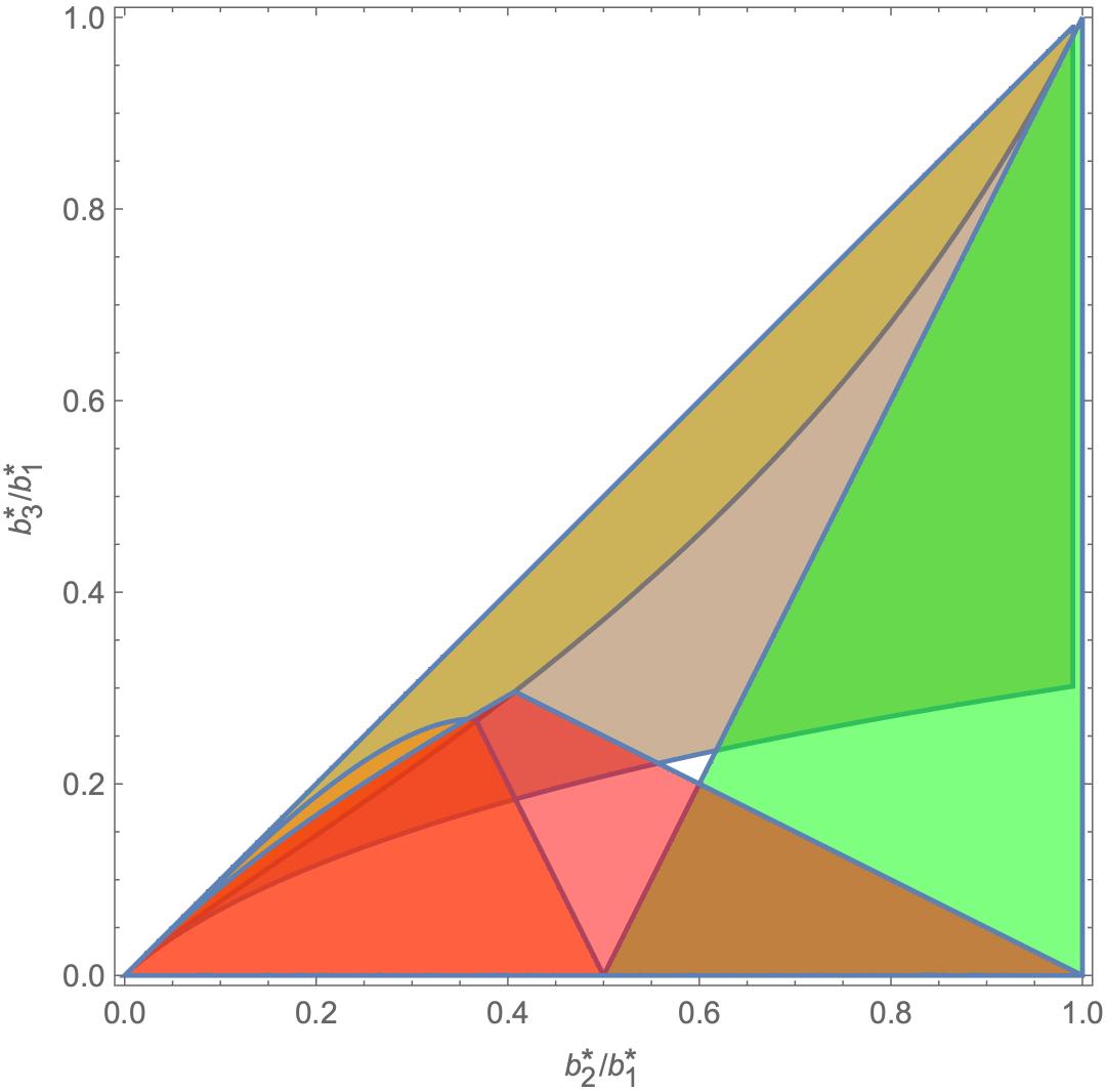
Figure 1: Superposition of the regions of existence of the five Riemann ellipsoids in the plane $b_{2}^{\ast}/b_{1}^{\ast}$–$b_{3}^{\ast}/b_{1}^{\ast}$

The five types of Riemann ellipsoids appear in Table 1, together with their regions of existence and their coordinates in the reduced space. The canonical basis of ${\mathbb{R}}^{3}$ is denoted as $\{e_{1},e_{2},e_{3}\}$.

Table 1: The first column shows the five types of Riemann ellipsoids. In the second column regions of existence in the plane $b_{2}^{\ast}/b_{1}^{\ast}$–$b_{3}^{\ast}/b_{1}^{\ast}$ are indicated. The third column accounts for the vectors $\mu^{\pm}_{\alpha}(b^{\ast})$ standing for $\eta_{l}(b^{\ast})$, $\eta_{r}(b^{\ast})$ such that the coordinates in $S_{L}^{2}\times S_{R}^{2}$ become $(\mu^{+}_{\alpha}(b^{\ast}),\mu^{-}_{\alpha}(b^{\ast}))$ or $(\mu^{-}_{\alpha}(b^{\ast}),\mu^{+}_{\alpha}(b^{\ast}))$. Hence, the coordinates of an ellipsoid of type $\alpha$ in $P_{L,R}$ are $(b^{\ast},0,\mu^{+}_{\alpha}(b^{\ast}),\mu^{-}_{\alpha}(b^{\ast}))$ or $(b^{\ast},0,\mu^{-}_{\alpha}(b^{\ast}),\mu^{+}_{\alpha}(b^{\ast}))$

Type ($\alpha$)	Region $(b_{2}^{\ast}/b_{1}^{\ast},b_{3}^{\ast}/b_{1}^{\ast})$	$\mu^{\pm}_{\alpha}(b^{\ast})$
$S_{2}$	${\mathcal{B}}_{S_{2}}$	$N^{S}_{\pm}(b_{1}^{\ast},b_{2}^{\ast},b_{3}^{\ast})e_{2}$
$S_{3}$	${\mathcal{B}}_{S_{3}}$	$N^{S}_{\pm}(b_{1}^{\ast},b_{3}^{\ast},b_{2}^{\ast})e_{3}$
I	${\mathcal{B}}_{\rm I}$	$N^{R}_{\pm}(b_{1}^{\ast},b_{3}^{\ast},b_{2}^{\ast})e_{1}+N^{R}_{\pm}(b_{3}^{\ast},b_{1}^{\ast},b_{2}^{\ast})e_{3}$
II	${\mathcal{B}}_{\rm II}$	$N^{R}_{\pm}(b_{1}^{\ast},b_{3}^{\ast},b_{2}^{\ast})e_{1}+N^{R}_{\mp}(b_{3}^{\ast},b_{1}^{\ast},b_{2}^{\ast})e_{3}$
III	${\mathcal{B}}_{\rm III}$	$N^{R}_{\pm}(b_{1}^{\ast},b_{2}^{\ast},b_{3}^{\ast})e_{1}+N^{R}_{\mp}(b_{2}^{\ast},b_{1}^{\ast},b_{3}^{\ast})e_{2}$

Remark 3.1.

The reduced system is invariant under both a ${\mathbb{Z}}_{2}$ and a ${\mathbb{Z}}_{4}$ action. A Riemann ellipsoid can be identified with the $({\mathbb{Z}}_{4}\times{\mathbb{Z}}_{2})$-orbit of an equilibrium of the reduced system, and it can consist of eight, four, or two equilibrium points on the reduced phase space, this depending on the number of zeroes vectors $\eta_{l}$, $\eta_{r}$ have; see more details in Proposition 4 of fasso2001stability. As ${\mathbb{Z}}_{2}$, ${\mathbb{Z}}_{4}$ are discrete symmetries, their application to further reduce the system would introduce singularities in the reduced space. In view of this, we do not reduce the system further and work with regular reduction techniques. Finally, following Fassò and Lewis, we distinguish between relative equilibria whose projections in $S_{L}^{2}\times S_{R}^{2}$ have coordinates $(\mu^{+}_{\alpha}(b^{\ast}),\mu^{-}_{\alpha}(b^{\ast}))$ or $(\mu^{-}_{\alpha}(b^{\ast}),\mu^{+}_{\alpha}(b^{\ast}))$, calling them adjoint equilibria.

In the following sections we describe the bifurcations of the equilibria. As a first step, their linear stability is determined. For that, we calculate the associated symplectic linear normal form and see that the equilibrium’s linearisation matrix is diagonalisable CushmanBurgoyne; LaubMeyer1974. Here we follow Markeev’s procedure Markeev to bring the linear Hamiltonian system (i.e. the one corresponding to the quadratic terms of the Hamilton function) to diagonal form. The algorithm is described in Appendix LABEL:Linearization and is designed for elliptic equilibria in Hamiltonian systems. The next step is the analysis of the non-linear stability and the bifurcations. We start by studying the stability of $S_{2}$-ellipsoids.

4 Stability of $S_{2}$-ellipsoids and the quasi-periodic pitchfork bifurcation in $\mathcal{B}_{S_{2}}$

The linear stability analysis of the $S_{2}$-ellipsoids is performed analytically without particularising for specific values of $(b_{2}^{\ast}/b_{1}^{\ast},b_{3}^{\ast}/b_{1}^{\ast})$ on a grid of points in the parametric plane, albeit the expressions are quite big. Nevertheless, the computations are much easier for these ellipsoids and for $S_{3}$ than they are for types I, II and III. The reason stems from the discrete symmetries of the problem and from the fact that the angular frequencies $\eta_{l}$ and $\eta_{r}$ are parallel to the same principal axis of the ellipsoid. This implies that the Hessian matrix and the associated linearisation matrix contain several zero blocks.

Recall that the region of existence for $S_{2}$-ellipsoids is defined by

$$\mathcal{B}_{S_{2}}=\Big{\{}b\in\mathcal{B}\,:\,G^{S}_{-}(b_{1}^{\ast},b_{2}^{\ast},b_{3}^{\ast})\geq 0\Big{\}},$$

where $\ignorespaces\mathcal{B}$ is given in (5). The region is represented in Fig. 2. It is enclosed between the lines $b_{2}^{\ast}=b_{3}^{\ast}$ and $G^{S}_{-}(b_{1}^{\ast},b_{2}^{\ast},b_{3}^{\ast})=0$. The green line is defined through the identity $G^{S}_{+}(b_{1}^{\ast},b_{2}^{\ast},b_{3}^{\ast})=G^{S}_{-}(b_{1}^{\ast},b_{2}^{\ast},b_{3}^{\ast})$ and corresponds to irrotational ellipsoids. On this line the Hamiltonian equation gets reduced to a system with three degrees of freedom. Above the line the two momenta of the ellipsoids are counter-parallel, whereas they are co-parallel below the curve.

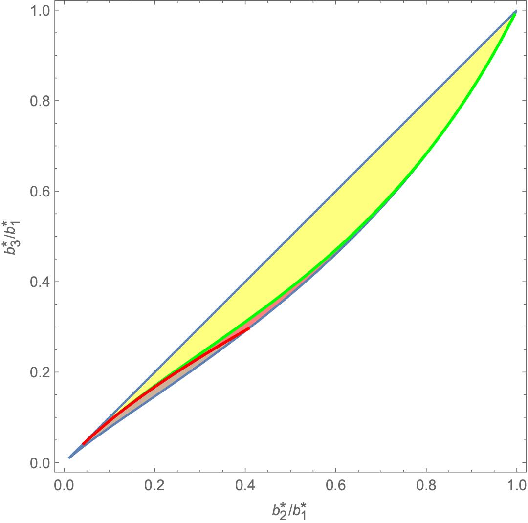
Figure 2: ${\mathcal{B}}_{S_{2}}$: Region of existence of the $S_{2}$-Riemann ellipsoids in the parametric plane $b_{2}^{\ast}/b_{1}^{\ast}$–$b_{3}^{\ast}/b_{1}^{\ast}$. The green line ( $G^{S}_{+}(b_{1}^{\ast},b_{2}^{\ast},b_{3}^{\ast})=G^{S}_{-}(b_{1}^{\ast},b_{2}^{\ast},b_{3}^{\ast})$) corresponds to the irrotational ellipsoids, whereas the red-one ($G=0$) accounts for a quasi-periodic Hamiltonian pitchfork bifurcation of co-parallel $S_{2}$-ellipsoids. In the yellow subregion the ellipsoids are Liapunov stable, while in the pink one they are linearly stable and in the brown one they are unstable

The region is divided into three sub-regions with different dynamics. Counter-parallel $S_{2}$-ellipsoids are Liapunov stable, as Riemann already stated Riemann. Co-parallel $S_{2}$-ellipsoids result to be linearly stable with indefinite quadratic Hamiltonian function, thus their Liapunov stability is not known from the linear analysis and a non-linear investigation is due.

We prove that co-parallel ellipsoids undergo a Hamiltonian pitchfork bifurcation of quasi-periodic nature. The red curve ($G=0$) corresponds to a supercritical quasi-periodic pitchfork bifurcation of invariant $3$-tori. An elliptic $3$-torus above the curve becomes parabolic on $G=0$ and then it turns hyperbolic when crossing the bifurcation line. Additionally, two elliptic $3$-tori are born when the first torus changes its stability. Furthermore, the appearance of the elliptic tori is associated to a global bifurcation involving type-III ellipsoids and it will be described in Section LABEL:global. The proof of the pitchfork bifurcation of invariant tori is partially based on KAM theory. We follow hanssmann2006local (Section 4.1), but references LitvakHinenzonRomKedar2002; LitvakHinenzonRomKedar2002Nonlinearity are also illustrative.

The values of $\mu^{\pm}_{S_{2}}(b^{\ast})$ introduced in the previous section are

$$N^{S}_{\pm}(b_{1}^{\ast},b_{2}^{\ast},b_{3}^{\ast})e_{2}=\left(0,\mbox{$\frac{1}{2}$}\Big{(}\sqrt{G^{S}_{+}(b_{1}^{\ast},b_{2}^{\ast},b_{3}^{\ast})}\pm\sqrt{G^{S}_{-}(b_{1}^{\ast},b_{2}^{\ast},b_{3}^{\ast})}\Big{)},0\right),$$ (13)

see Table 1. We check that these expressions are well defined. Due to the fact that in the $\mathcal{B}_{S_{2}}$-region $\ignorespaces G^{S}_{-}(b_{1}^{\ast},b_{2}^{\ast},b_{3}^{\ast})\geq 0$ holds, the only thing that should be checked is ${G^{S}_{+}(b_{1}^{\ast},b_{2}^{\ast},b_{3}^{\ast})}\geq 0.$ From (11) we obtain

$$\begin{array}[]{lcl}G_{+}^{S}(b_{1}^{\ast},b_{2}^{\ast},b_{3}^{\ast})&=&\displaystyle\frac{(b_{1}^{\ast 2}b_{2}^{\ast}-1)^{4}}{b_{1}^{\ast 6}b_{2}^{\ast 5}}\Big{(}\big{(}b_{2}^{\ast 2}+b_{1}^{\ast 4}b_{2}^{\ast 4}+b_{1}^{\ast 2}(b_{2}^{\ast 3}-1)\big{)}C_{1}(b_{1}^{\ast},b_{2}^{\ast},b_{3}^{\ast})\\ &&\hskip 59.75095pt+\,\big{(}b_{1}^{\ast 2}b_{2}^{\ast}(b_{2}^{\ast 3}+1)\big{)}C_{2}(b_{1}^{\ast},b_{2}^{\ast},b_{3}^{\ast})\Big{)}.\end{array}$$

Note that $C_{i}(b^{\ast})$ are non-negative, as they are integrals of positive functions. Additionally, using (5) it is readily deduced that the terms factorising $C_{1}(b^{\ast})$ and $C_{2}(b^{\ast})$ are also positive. Hence, $G_{+}^{S}(b_{1}^{\ast},b_{2}^{\ast},b_{3}^{\ast})$ is non-negative in this region.

The following theorem is the main result regarding the dynamics of $S_{2}$-ellipsoids.

Theorem 4.1.

Region $\mathcal{B}_{S_{2}}$ is divided into three sub-regions with the following features:

1. The first subregion is bounded by the lines $b_{2}^{\ast}=b_{3}^{\ast}$ and $G^{S}_{+}(b_{1}^{\ast},b_{2}^{\ast},b_{3}^{\ast})=G^{S}_{-}(b_{1}^{\ast},b_{2}^{\ast},b_{3}^{\ast})$ (green curve in Fig. 2) and corresponds with counter-parallel $S_{2}$-ellipsoids. The counter-parallel $S_{2}$-ellipsoids in the interior of this subregion and the irrotational ones on the green curve are Liapunov stable.
   

2. The second subregion is delimited above by the line $G^{S}_{+}(b_{1}^{\ast},b_{2}^{\ast},b_{3}^{\ast})=G^{S}_{-}(b_{1}^{\ast},b_{2}^{\ast},b_{3}^{\ast})$ and below by the curves $\ignorespaces G=0$ and $G^{s}_{-}(b_{1}^{\ast},b_{2}^{\ast},b_{3}^{\ast})=0$:
   

   • The co-parallel $S_{2}$-ellipsoids are linearly stable inside this region and on this part of the line $G^{s}_{-}(b_{1}^{\ast},b_{2}^{\ast},b_{3}^{\ast})=0$.

   • The curve $\ignorespaces G=0$ (red line in Fig. 2) corresponds to a Hamiltonian pitchfork bifurcation of quasi-periodic nature.

3. The third subregion is bounded from above by the curve $G=0$ and by $G^{s}_{-}(b_{1}^{\ast},b_{2}^{\ast},b_{3}^{\ast})=0$ from below and corresponds with co-parallel $S_{2}$-ellipsoids. Inside this region the ellipsoids are unstable.

Proof: We choose the ellipsoid with $(S^{2}_{L}\times S^{2}_{R})$-coordinates $(\mu^{+}_{S_{2}}(b^{\ast}),\mu^{-}_{S_{2}}(b^{\ast}))$, the study being the same for its adjoint ellipsoid. Parameters $L$, $R$ satisfy

$$L=N^{S}_{+}(b^{\ast}),\quad R=|N^{S}_{-}(b^{\ast})|,$$

where $N^{S}_{\pm}$ has been introduced in (13). Counter-parallel $S_{2}$-ellipsoids are represented by the equilibrium with coordinates $(b_{1}^{\ast},b_{2}^{\ast},0,0,0,-L,0,0,R,0)$. Thus, the projection onto $S^{2}_{L}\times S^{2}_{R}$ corresponds to the South-North poles of the two-spheres. The coordinates of co-parallel ellipsoids are $(b_{1}^{\ast},b_{2}^{\ast},0,0,0,L,0,0,R,0)$ and the projection onto $S^{2}_{L}\times S^{2}_{R}$ corresponds to the North-North poles of the two-spheres.

We start by determining the linear stability. The first step is shifting the equilibrium to the origin. For that, the following transformation is applied

$$(\bar{b},\bar{c},q_{1},q_{2},p_{1},p_{2})\rightarrow(b,c,\eta_{l},\eta_{r}),$$

where $\bar{b}=(\bar{b}_{1},\bar{b}_{2})$, $\bar{c}=(\bar{c}_{1},\bar{c}_{2})$ and

$$\begin{array}[]{lcl}b_{i}&=&b_{i}^{\ast}+{\bar{b}_{i}},\quad c_{i}={\bar{c}_{i}},\\[4.30554pt] m_{1}&=&\pm q_{1}\sqrt{L-\frac{q_{1}^{2}+p_{1}^{2}}{4}},\quad m_{2}=\mp L\pm\frac{q_{1}^{2}+p_{1}^{2}}{2},\quad m_{3}=p_{1}\sqrt{L-\frac{q_{1}^{2}+p_{1}^{2}}{4}},\\[4.30554pt] m_{4}&=&-q_{2}\sqrt{R-\frac{q_{2}^{2}+p_{2}^{2}}{4}},\quad m_{5}=R-\frac{q_{2}^{2}+p_{2}^{2}}{2},\quad m_{6}=p_{2}\sqrt{R-\frac{q_{2}^{2}+p_{2}^{2}}{4}},\end{array}$$

with the upper sign applying for counter-parallel ellipsoids and the lower one for co-parallel ellipsoids, see also the similar approach followed in fasso2001stability.

Notice that the local coordinates $(q_{1},q_{2},p_{1},p_{2})$ are canonical, as they preserve the Poisson structure associated to $m_{i}$, $i=1,\ldots,6$; thus, the whole transformation is symplectic.

Naming $u=(\bar{b},q_{1},q_{2},\bar{c},p_{1},p_{2})$, the set of Cartesian coordinates (also said rectangular), the next step is performing a Taylor expansion around $u=0$ up to polynomials of degree two. We determine the quadratic form $H_{2}(u)=\frac{1}{2}\,u^{T}\cdot(-{\mathcal{J}}_{8}{\mathcal{L}})\cdot u$, where ${\mathcal{J}}_{8}$ is the usual $(8\times 8)$-skew symmetric matrix, whereas $H_{2}$ refers to the Hamiltonian function of the linearised system around $u=0$ with linearisation matrix ${\mathcal{L}}$. The entries of this matrix are provided explicitly in Appendix LABEL:CoefficientsL for the co-parallel case. Notice that they are similar in the counter-parallel regime and that they have been placed in the Mathematica file supplied with the paper.

Next, we apply Markeev’s algorithm described in Appendix LABEL:Linearization to bring $H_{2}$ to normal form. We arrive at the following conclusions:

1. Counter-parallel ellipsoids are Liapunov stable because the Hamiltonian corresponding to the linearised system in the normal-form coordinates $z=(x_{1},x_{2},x_{3},y_{1},y_{2},y_{3})$ becomes

   $$H_{2}(z)=\frac{\omega_{1}}{2}(x_{1}^{2}+y_{1}^{2})+\frac{\omega_{2}}{2}(x_{2}^{2}+y_{2}^{2})+\frac{\omega_{3}}{2}(x_{3}^{2}+y_{3}^{2})+\frac{\omega_{4}}{2}(x_{4}^{2}+y_{4}^{2}),$$

   where the frequencies $\omega_{i}$ appear in (LABEL:omegas) and have to be understood such that the associated coefficients $\ell_{i,j}$ are those specific for the counter-parallel regime of the $S_{2}$-ellipsoids. The entries $\ell_{i,j}$ are given in the Mathematica file. In this subregion of $\mathcal{B}_{S_{2}}$ the transformation matrix ${\mathcal{T}}$ appearing in Appendix LABEL:Linearization is real and the $\omega_{i}$, $i=1,\ldots,4$, coefficients are positive. Thus, applying Dirichlet Stability Theorem meyeroffin, Liapunov stability is achieved.
   

   On the boundary of the subregion, i.e. on the curve $G^{S}_{+}(b_{1}^{\ast},b_{2}^{\ast},b_{3}^{\ast})=G^{S}_{-}(b_{1}^{\ast},b_{2}^{\ast},b_{3}^{\ast})$ (green line in Fig. 2) the system has three degrees of freedom. We set $m_{1}=m_{2}=m_{3}=0$ and take $u=(\bar{b},q_{2},\bar{c},p_{2})$. The equilibrium has coordinates $(b_{1}^{\ast},b_{2}^{\ast},0,0,0,R,0)$ and the symplectic matrix ${\mathcal{T}}_{I}$ is defined accordingly. We note that all matrices ${\mathcal{L}}_{I}$, ${\mathcal{T}}_{I}$ and ${\mathcal{J}}_{6}$ involved are $(6\times 6)$-dimensional. The normal-form Hamiltonian truncated at degree two in this case is

   $$H_{2}(z)=\frac{\omega_{1}}{2}(x_{1}^{2}+y_{1}^{2})+\frac{\omega_{2}}{2}(x_{2}^{2}+y_{2}^{2})+\frac{\omega_{3}}{2}(x_{3}^{2}+y_{3}^{2}).$$

   The frequencies $\omega_{i}$ appearing in (LABEL:omegas) satisfy $\omega_{i}>0$ for $i=1,2,3$. Thereby, Liapunov stability also holds on the boundary of this subregion.
   

2. (and (iii)) Now we focus on co-parallel ellipsoids. The linear normal form is determined by applying Markeev’s approach as in item i. That being said, we wish to obtain a normal-form Hamiltonian that remains valid not only for the linearly stable part, but also for the unstable one. Thus, we need to make a slight modification in the calculation of matrix ${\mathcal{T}}$. Indeed, it is enough to do $x_{4}\rightarrow\sqrt{\omega_{4}}x_{4}$, $y_{4}\rightarrow y_{4}/\sqrt{\omega_{4}}$. By applying this change and doing some simplifications the resulting matrix, that we also name ${\mathcal{T}}$ is, is real and well defined everywhere above, below and on the red line. (The $\omega_{4}$ in the denominator of $y_{4}$ compensates with a factor in the denominator that also vanishes on the bifurcation line leading to a valid formula which makes sense even when $\omega_{4}=0$.) The final linear transformation remains symplectic, and is given in Appendix LABEL:Linearization.
   

   Matrix ${\mathcal{T}}$ lies in the range of the so called versal normal form. The theory was developed by Arnold Arnold to overcome the difficulty that for matrices that depend on parameters their transformations into Jordan canonical form could become singular. In our context, $\mathcal{T}$ depends smoothly on $\omega_{4}$ and it is real and non-singular in a neighbourhood, at least in a narrow strip surrounding the curve $G=0$.
   

   The transformed quadratic Hamiltonian function is

   $$H_{2}(z)=\frac{\omega_{1}}{2}(x_{1}^{2}+y_{1}^{2})+\frac{\omega_{2}}{2}(x_{2}^{2}+y_{2}^{2})+\frac{\omega_{3}}{2}(x_{3}^{2}+y_{3}^{2})-\frac{1}{2}(\omega_{4}^{2}x_{4}^{2}+y_{4}^{2}),$$

   with $\omega_{i}$ given in (LABEL:omegas), where this time $\ell_{i,j}$ are provided in an explicit way in Appendix LABEL:CoefficientsL. We stress that $\omega_{i}>0$ for $i=1,2,3$, while $\omega_{4}$ can be positive, pure imaginary with negative imaginary part or zero. More specifically $\omega_{4}>0$ for co-parallel ellipsoids above the bifurcation line $G=0$ (i.e., the red line in Fig. 2), whereas $\omega_{4}=\imath\bar{\omega}_{4}$, $\bar{\omega_{4}}<0$ for co-parallel ellipsoids below the red curve, and $\omega_{4}=0$ on the curve $G=0$. Actually, $G=0$ is equivalent to $\omega_{4}=0$ at the points of the parametric plane where the bifurcation takes place. Thereby, both above and below the line $G=0$ the Hamiltonian is semisimple.
   

   The origin $z=0$ is linearly stable above $G=0$, as the linearisation is of the type centre $\times$ centre $\times$ centre $\times$ centre with three positive signs in front of the $\omega_{i}>0$ and one negative. Below the red curve, since

   $$-\mbox{$\frac{1}{2}$}(\omega_{4}^{2}x_{4}^{2}+y_{4}^{2})=-\mbox{$\frac{1}{2}$}(-\bar{\omega}_{4}^{2}x_{4}^{2}+y_{4}^{2}),\quad\mbox{with}\,\,\bar{\omega}_{4}^{2}>0,$$

   the equilibrium is unstable with linearisation centre $\times$ centre $\times$ centre $\times$ saddle. On the red curve the Hamiltonian is no longer semisimple, as it has the nilpotent term $-y_{4}^{2}/2$.
   

   In order to prove that a quasi-periodic Hamiltonian pitchfork bifurcation takes place we need to determine the non-linear terms up to degree four. For that, we extend the computation of the normal form up to quartic terms in the $z$ coordinates and express the normal form in complex/real-symplectic coordinates, say $Z=(X_{1},X_{2},X_{3},X_{4},Y_{1},Y_{2},Y_{3},Y_{4})$, such that

   $$\begin{array}[]{lcl}x_{i}&=&\mbox{$\frac{1}{\sqrt{2}}$}(X_{i}+\imath Y_{i}),\quad y_{i}=\mbox{$\frac{1}{\sqrt{2}}$}(\imath X_{i}+Y_{i}),\quad i=1,\ldots,3,\\[3.87498pt] x_{4}&=&X_{4},\quad y_{4}=Y_{4}.\end{array}$$ (14)

   Then,

   $$H_{2}(Z)=\imath\omega_{1}X_{1}Y_{1}+\imath\omega_{2}X_{2}Y_{2}+\imath\omega_{3}X_{3}Y_{3}-\mbox{$\frac{1}{2}$}(\omega_{4}^{2}X_{4}^{2}+Y_{4}^{2}).\\$$

   It is time to apply the linear changes passing from the $u$ coordinates to the $Z$ and execute two steps of the Lie transformation method Deprit, proceeding in a symbolic fashion. The first order of the generating function, ${\mathcal{W}}_{1}$, is determined in such a way that the associated normal form, $H_{1}$, be zero. For that, we deal with the homological equation solving 120 linear equations with 120 unknowns (these unknowns are the coefficients of the terms of ${\mathcal{W}}_{1}$, i.e., monomials of degree three in $Z$). Cubic terms are neither present in the Hamiltonian funciton written in normal-form coordinates. This is due to the reversible character of the perturbation in case of type-$S$ ellipsoids.
   

   For computing the normal-form Hamiltonian, say $H_{4}$, and the associated generating function ${\mathcal{W}}_{2}$ we impose that the terms in the normal form are combinations of $X_{1}Y_{1}$, $X_{2}Y_{2}$, $X_{3}Y_{3}$, $X_{4}^{2}$. As $H_{4}$ is of degree four in $Z$ (by an abuse of notation we also name $Z$ the transformed coordinates), we set

   $$\begin{array}[]{lcl}H_{4}(Z)&=&Q_{1}(X_{1}Y_{1})^{2}+Q_{2}(X_{2}Y_{2})^{2}+Q_{3}(X_{3}Y_{3})^{2}+Q_{4}(X_{4}^{2})^{2}\\[3.87498pt] &&+\,Q_{5}X_{1}Y_{1}X_{2}Y_{2}+Q_{6}X_{1}Y_{1}X_{3}Y_{3}+Q_{7}X_{2}Y_{2}X_{3}Y_{3}\\[3.87498pt] &&+\,Q_{8}X_{1}Y_{1}X_{4}^{2}+Q_{9}X_{2}Y_{2}X_{4}^{2}+Q_{10}X_{3}Y_{3}X_{4}^{2}.\end{array}$$

   One has to expect a transformed Hamiltonian like $H_{4}$ due to the nilpotent term in $H_{2}$ when $\omega_{4}=0$, see meyeroffin. The $Q_{i}$ coefficients $(i=1,\ldots,10)$ and the ones forming the function ${\mathcal{W}}_{2}$ are determined by solving a consistent underdetermined linear system with 330 equations and 340 unknowns. Out of all unknowns, 330 correspond to the coefficients of ${\mathcal{W}}_{2}$ written in terms of the monomials of degree four in $Z$, and the other ten are the $Q_{i}$.
   

   The transformation is well defined excepting certain resonance values. We determine the resonances by taking the denominators in the generating functions ${\mathcal{W}}_{1}$ and ${\mathcal{W}}_{2}$, evaluating them along the bifurcation line ($\omega_{4}=0$) and selecting the ones that pass through zero. There are two resonances of order $3$ and one of orders $2$ and $4$, specifically

   $$-\omega_{1}+\omega_{3},\,-\omega_{1}+2\,\omega_{2},\,-2\,\omega_{2}+\omega_{3},\,-\omega_{1}+3\,\omega_{2}.$$

   They are shown in Fig. 3. The order-two resonance is $-\omega_{1}+\omega_{3}$. The order-three ones are $-\omega_{1}+2\,\omega_{2}$ and $-2\,\omega_{2}+\omega_{3}$. The resonance of order $4$ is $-\omega_{1}+3\,\omega_{2}$. Consequently, in order to avoid the appearance of vanishing denominators in the expressions, we need to remove from the line $G=0$ those points $(b_{2}^{\ast}/b_{1}^{\ast},b_{3}^{\ast}/b_{1}^{\ast})$ where the linear combinations of the frequencies become zero, since for these points of the parametric plane the approach is not valid. Furthermore, by continuity of the formulae with respect to the parameters $b^{\ast}$, we discard small neighbourhoods (balls centred at the points where the denominators are exactly zero), since some terms in the generating functions become unbounded there. More precisely, $-\omega_{1}+\omega_{3}=0$ for $b_{2}^{\ast}/b_{1}^{\ast}\approx 0.3602$, $-\omega_{1}+2\,\omega_{2}=0$ for $b_{2}^{\ast}/b_{1}^{\ast}\approx 0.2716$, $-2\,\omega_{2}+\omega_{3}=0$ for $b_{2}^{\ast}/b_{1}^{\ast}\approx 0.2802$ and $-\omega_{1}+3\,\omega_{2}=0$ for $b_{2}^{\ast}/b_{1}^{\ast}\approx 0.1518$ and the values of $b_{3}^{\ast}/b_{1}^{\ast}$ are determined after solving the equation $G=0$.
   

   

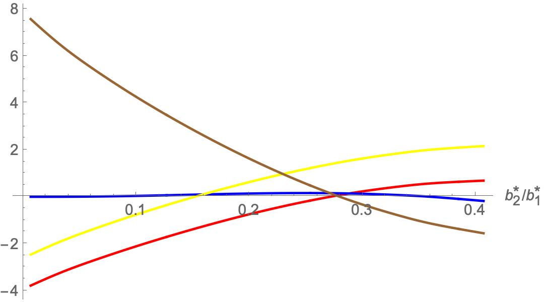
   Figure 3: Resonances of different orders. Order 2: blue, $-\omega_{1}+\omega_{3}$. Order 3: red, $-\omega_{1}+2\,\omega_{2}$; brown, $-2\omega_{2}+\omega_{3}$. Order 4: yellow, $-\omega_{1}+3\,\omega_{2}$. Despite the blue curve looks very close to the axis $b_{2}^{\ast}/b_{1}^{\ast}$, it starts on the left taking the value $-\omega_{1}+\omega_{3}=7.44...\cdot 10^{-6}$ for $b_{2}^{\ast}/b_{1}^{\ast}\approx 0$, then, it increases reaching its maximum at around $b_{2}^{\ast}/b_{1}^{\ast}=0.24$ and decreases crossing the horizontal axis at a unique point around $b_{2}^{\ast}/b_{1}^{\ast}=0.3602$

   Next we check the specific conditions for establishing the occurrence of a supercritical quasi-periodic Hamiltonian pitchfork bifurcation on the curve $G=0$, see Theorem 4.13 in hanssmann2006local.
   

   We return to a real normal form by introducing the actions $I_{i}=\imath X_{i}Y_{i}$, $i=1,2,3$. The linearised system has as Hamiltonian function

   $$H_{2}(I,X_{4},Y_{4})=\omega_{1}I_{1}+\omega_{2}I_{2}+\omega_{3}I_{3}-\mbox{$\frac{1}{2}$}(\omega_{4}^{2}X_{4}^{2}+Y_{4}^{2}),\,\,\,\,I=(I_{1},I_{2},I_{3}).$$

   At this point we consider the truncated normal form $H^{4}=H_{2}+\frac{1}{2}H_{4}$ in terms of $I$, $X_{4}$, $Y_{4}$. We write it as

   $$\begin{array}[]{rcl}H^{4}(I,X_{4},Y_{4})&=&\omega_{1}I_{1}+\omega_{2}I_{2}+\omega_{3}I_{3}-\mbox{$\frac{1}{2}$}(\omega_{4}^{2}X_{4}^{2}+Y_{4}^{2})\\[3.87498pt] &&-\,\mbox{$\frac{1}{2}$}\left(Q_{1}I_{1}^{2}+Q_{2}I_{2}^{2}+Q_{3}I_{3}^{2}+Q_{5}I_{1}I_{2}+Q_{6}I_{1}I_{3}+Q_{7}I_{2}I_{3}\right.\\[3.87498pt] &&\left.\hskip 19.34766pt+\,\imath\,(Q_{8}I_{1}+Q_{9}I_{2}+Q_{10}I_{3})X_{4}^{2}-Q_{4}X_{4}^{4}\right),\end{array}$$ (15)

   which is a real function because $Q_{8}$, $Q_{9}$, $Q_{10}$ are pure imaginary while the other $Q_{i}$ are real.
   

   Notice that the coefficient of $Y_{4}^{2}$ in $H^{4}$ is negative. Besides, we take a careful look at the coefficients of $X_{4}^{2}$ and $X_{4}^{4}$, respectively,

   $$-\mbox{$\frac{1}{2}$}\left(\omega_{4}^{2}+\imath(Q_{8}I_{1}+Q_{9}I_{2}+Q_{10}I_{3})\right),\quad\mbox{$\frac{1}{2}$}Q_{4}.\\$$

   Firstly, the coefficient of $X_{4}^{2}$ is zero for $I=0$, $\omega_{4}=0$ but it does not vanish when $\omega_{4}\neq 0$ and $I=0$, that is, in a neighbourhood of the line $G=0$. Proving that $Q_{4}\neq 0$ when $\omega_{4}=0$ requires more effort. We need to prove that both coefficients vanish only when $\omega_{4}=0$. We also check that the coefficient of $X_{4}^{4}$ is different from zero. Let us stress that $Q_{4}$ is computed in an explicit way on the whole line $G=0$ and also in a neighbourhood of it, and it is given in terms of $b^{\ast}$ and supplied in the Mathematica file. However, for the sake of proving that it does not vanish on the bifurcation line we proceed by replacing $Q_{4}$ in terms of the values $b^{\ast}$ take on the line $G=0$. This step is numerical but we have performed it with very high precision of the calculations. We conclude that $Q_{4}<0$ in all points of the bifurcation line, see Fig. 4. By continuity of the formulae with respect to the parameters and variables it is also negative on a narrow strip of the bifurcation line in the parametric plane. This bifurcation is of supercritical type as the coefficient of $Y_{4}^{2}$ is negative and the coefficient of $X_{4}^{4}$ remains negative as well.
   

   

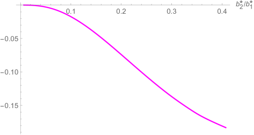
   Figure 4: Coefficient $Q_{4}$ evaluated along the line $G=0$. It is always below the horizontal axis. In fact, it starts taking the value $Q_{4}=-7.341...\cdot 10^{-6}$ for $b_{2}^{\ast}/b_{1}^{\ast}\approx 0$, and it is a decreasing function. Thus, $Q_{4}$ is negative for $b^{\ast}$ on the bifurcation line

   At this point we need to prove the persistence under perturbation of the invariant tori related to the bifurcation. For this purpose we introduce

   $$\tilde{c}(I)=-\mbox{$\frac{1}{2}$}\omega_{4}^{2}-\mbox{$\frac{\imath}{2}$}(Q_{8}I_{1}+Q_{9}I_{2}+Q_{10}I_{3}),\quad\tilde{\omega}_{i}(I)=\frac{\partial H^{4}(I,0,0)}{\partial I_{i}},$$

   and define the map $\xi:I\rightarrow\left(\tilde{c}(I),\tilde{\omega}_{1}(I),\tilde{\omega}_{2}(I),\tilde{\omega}_{3}(I)\right)$. Notice that $\tilde{c}(I)$ is taken as the coefficient of $X_{4}^{2}$ in $H^{4}$.
   

   We have to prove that $\xi$ a submersion at $\omega_{4}=0$, i.e. that the map is differentiable and the differential is surjective everywhere. Following hanssmann2006local, on the one hand we get $D\tilde{c}(0)=-\frac{\imath}{2}(Q_{8},Q_{9},Q_{10})\neq(0,0,0)$ along the curve $G=0$, excepting at the resonance combinations which lead to very small or null denominators. More precisely, the evaluation of the norm of $D\tilde{c}(0)$ on a grid of points along the curve $G=0$, remains positive and its minimum value is approximately $0.1617$. On the other hand, we build the ($3\times 3$)-matrix $\mathtt{M}$ whose first row is $(\tilde{\omega}_{1}(I),\tilde{\omega}_{2}(I),\tilde{\omega}_{3}(I))$, the second and third rows are the partial derivatives of the first row with respect to $I_{1}$ and $I_{3}$. The determinant of $\mathtt{M}$ at $I=0$ yields

   $$\mbox{$\frac{1}{4}$}\left(\omega_{1}(2\,Q_{3}Q_{5}-Q_{6}Q_{7})+\omega_{2}(Q_{6}^{2}-4\,Q_{1}Q_{3})+\omega_{3}(2\,Q_{1}Q_{7}-Q_{5}Q_{6})\right).$$

   This expression remains positive in a fine grid of points $b^{\ast}$ chosen homogeneously along the bifurcation curve $\omega_{4}=0$. We have to exclude the resonance values, where the normal-form computations do not make sense. Then, we conclude that the map $\xi$ is a submersion. The related calculations are provided in the Mathematica file.
   

   This gives the persistence of the invariant tori that interplay in the bifurcation.

Remark 4.2.

Determining the validity of the linear normal-form transformations, that is, whether ${\mathcal{T}}$, ${\mathcal{T}}_{I}$ are real matrices with non-vanishing denominators in the corresponding subregions of $\mathcal{B}_{S_{2}}$ where they are built, is not easy to accomplish. The same happens with the frequencies $\omega_{i}$. For instance, they are strictly positive for the ellipsoids of item i in the proof. Thus, one concludes Liapunov stability. In fact, we have all the associated expressions given explicitly in terms of $b^{\ast}$, but they are too big so that we can check our requisites. One can prove some partial results, for instance: $\omega_{1}>\omega_{2}$, $\omega_{3}>|\omega_{4}|$. An alternative is checking the validity of our claim on a fine grid in ${\mathcal{B}}_{S_{2}}$, with the values $\ell_{i,j}$ take accordingly to the subregion we are considering. This can be performed with Mathematica using the routine RegionPlot[], that makes plots of the provided formulae on specified regions in a two-dimensional grid. The approach is numerical but one can use high precision for the internal calculations. For instance, one can check that $\omega_{i}>0$ on the green line and above it. The approach is similar for the behaviour of $\omega_{4}$ close to the bifurcation line. Proceeding like this we observe that the constructions we present are all right.

Remark 4.3.

The invariant $3$-tori persisting in the co-parallel region (above and below the bifurcation line) are surrounded by families of invariant Lagrangian $4$-tori. This is established applying the standard Kolmogorov’s non-degeneracy condition.

Remark 4.4.

The principal terms of the invariant $3$ or $4$-tori that persist the small perturbations are trivially derived from Hamiltonian $H^{4}$ in (15) in the normal-form coordinates $I$, $X_{4}$,$Y_{4}$. It is possible to obtain them in the original coordinates by undoing the normal-form transformations.

5 Stability of $S_{3}$-ellipsoids

We deal with the $S_{3}$-ellipsoids. Riemann already proved that they are Liapunov stable Riemann. Our contribution stems from the fact that the calculations are symbolically in the entire region of existence. This time $\mu^{\pm}_{S_{3}}(b^{\ast})$ of Table 1 is

$$N^{S}_{\pm}(b_{1}^{\ast},b_{3}^{\ast},b_{2}^{\ast})e_{3}=\left(0,0,\mbox{$\frac{1}{2}$}\Big{(}\sqrt{G^{S}_{+}(b_{1}^{\ast},b_{3}^{\ast},b_{2}^{\ast})}\pm\sqrt{G^{S}_{-}(b_{1}^{\ast},b_{3}^{\ast},b_{2}^{\ast})}\Big{)}\right).$$ (16)

The region of the parametric plane where these Riemann ellipsoids exist is given by

$${\mathcal{B}}_{S_{3}}=\Big{\{}b\in{\mathcal{B}}\,:\,G_{+}^{S}(b_{1}^{\ast},b_{3}^{\ast},b_{2}^{\ast})\geq 0\Big{\}}$$

and is represented in Fig. 5. Condition $G_{-}^{S}(b_{1}^{\ast},b_{3}^{\ast},b_{2}^{\ast})\geq 0$ is satisfied because

$$\begin{array}[]{lcl}G_{-}^{S}(b_{1}^{\ast},b_{3}^{\ast},b_{2}^{\ast})&=&\displaystyle\frac{(b_{1}^{\ast}-b_{2}^{\ast})^{4}}{b_{1}^{\ast 3}b_{2}^{\ast 3}}\Big{(}\big{(}b_{1}^{\ast 4}b_{2}^{\ast 4}+b_{1}^{\ast}b_{2}^{\ast}-b_{1}^{\ast 2}-b_{2}^{\ast 2}\big{)}C_{1}(b_{1}^{\ast},b_{3}^{\ast},b_{2}^{\ast})\\ &&\displaystyle\hskip 51.21504pt+\,\big{(}b_{1}^{\ast 3}b_{2}^{\ast 3}-1\big{)}C_{2}(b_{1}^{\ast},b_{3}^{\ast},b_{2}^{\ast})\Big{)}\end{array}$$

and $C_{1}(b_{1}^{\ast},b_{3}^{\ast},b_{2}^{\ast})$, $C_{2}(b_{1}^{\ast},b_{3}^{\ast},b_{2}^{\ast})$, together with their coefficients, are also positive by condition (5). In so doing, the $S_{3}$-ellipsoids are properly defined in ${\mathcal{B}}_{S_{3}}$.

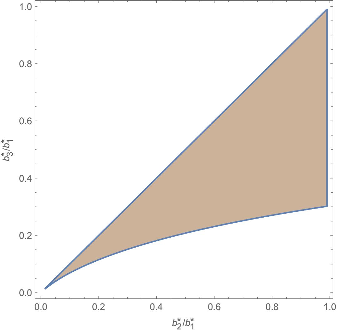
Figure 5: ${\mathcal{B}}_{S_{3}}$: Region of existence of the $S_{3}$-Riemann ellipsoids

We state the main result of this section.

Theorem 5.1.

$S_{3}$-ellipsoids are Liapunov stable equilibria in their entire region of existence.

Proof: We take the cue from the scheme pursued in the proof of Theorem 4.1. The coordinates of the $S_{3}$-ellipsoids are $(b_{1}^{\ast},b_{2}^{\ast},0,0,0,0,-L,0,0,R)$, with $L$ and $R$ as in the case of $S_{2}$-ellipsoids. Projecting them onto $S^{2}_{L}\times S^{2}_{R}$ they correspond to the South-North poles of the two-spheres. Hence, $S_{3}$-ellipsoids are counter-parallel and the following change to symplectic variables is applied

$$(\bar{b},\bar{c},q_{1},q_{2},p_{1},p_{2})\rightarrow(b,c,\eta_{l},\eta_{r}),$$

where $\bar{b}=(\bar{b}_{1},\bar{b}_{2})$, $\bar{c}=(\bar{c}_{1},\bar{c}_{2})$ and

$$\begin{array}[]{lcl}b_{i}&=&b_{i}^{\ast}+{\bar{b}_{i}},\quad c_{i}={\bar{c}_{i}},\\[4.30554pt] m_{1}&=&p_{1}\sqrt{L-\frac{q_{1}^{2}+p_{1}^{2}}{4}},\quad m_{2}=q_{1}\sqrt{L-\frac{q_{1}^{2}+p_{1}^{2}}{4}},\quad m_{3}=-L+\frac{q_{1}^{2}+p_{1}^{2}}{2},\\[5.59721pt] m_{4}&=&p_{2}\sqrt{R-\frac{q_{2}^{2}+p_{2}^{2}}{4}},\quad m_{5}=-q_{2}\sqrt{R-\frac{q_{2}^{2}+p_{2}^{2}}{4}},\quad m_{6}=R-\frac{q_{2}^{2}+p_{2}^{2}}{2}.\end{array}$$

In this manner we translate the equilibrium to the origin. Then, a Taylor expansion up to degree 2 is computed in the coordinates $u$. The coefficients of the linearisation matrix ${\mathcal{L}}$ are similar to those given in Appendix LABEL:CoefficientsL for the $S_{2}$-ellipsoids in the co-parallel regime, and they are provided in the Mathematica file accompanied to this text. Next, we apply Markeev’s procedure described in Appendix LABEL:Linearization to bring the quadratic form $H_{2}(u)$ to normal form. The linearisation in Cartesian coordinates results to be

$$H_{2}(z)=\frac{\omega_{1}}{2}(x_{1}^{2}+y_{1}^{2})+\frac{\omega_{2}}{2}(x_{2}^{2}+y_{2}^{2})+\frac{\omega_{3}}{2}(x_{3}^{2}+y_{3}^{2})+\frac{\omega_{4}}{2}(x_{4}^{2}+y_{4}^{2}),$$

with $\omega_{i}$ appearing in (LABEL:omegas) and the corresponding $\ell_{i,j}$ are given in the Mathematica file. One has that $\omega_{i}>0$ for $i=1,\ldots,4$. Consequently, $S_{3}$-ellipsoids are Liapunov stable.

Remark 5.2.

Analogous considerations to those made in Remark 4.2 apply for the $S_{3}$-ellipsoids. They also apply in the bifurcation study of types-II and III ellipsoids.

6 Linear stability of type-I irrotational ellipsoids

This section is devoted to the analysis of the stability of type-I ellipsoids. Their existence domain is

$$\mathcal{B}_{{\rm I}}=\Big{\{}b\in\mathcal{B}\,:\,b_{1}^{\ast}\leq 2b_{2}^{\ast}-b_{3}^{\ast}\Big{\}},$$

and is represented in Fig. 6.

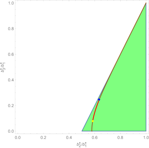
Figure 6: ${\mathcal{B}}_{{\rm{I}}}$: Region of existence of type-I Riemann ellipsoids. The curve corresponds to irrotational ellipsoids. In the red portion there is linear stability, whereas there is instability in the brown ones. The brown part continues to the point $(1,1)$. The yellow and blue points are likely to be Hamiltonian-Hopf bifurcations

Type-I ellipsoids can be linearly stable or unstable, passing from stable to unstable through bifurcation lines whose distribution may be very subtle fasso2001stability. We have not detected Liapunov stability in this region just from a linear analysis. It could arise after studying the non-linear terms, but this is far from obvious. The bifurcation lines likely correspond to quasi-periodic Hamiltonian-Hopf bifurcations broer2007quasi; meyeroffin. We do not present the analysis of these bifurcations in this section, as it is similar to the one we shall detail for type-III ellipsoids.

The procedure to study the linear stability of these ellipsoids follows the ideas of previous sections. We start by choosing the ellipsoid with $(S^{2}_{L}\times S^{2}_{R})$-coordinates $(\mu^{+}_{N}(b_{1}^{\ast},b_{3}^{\ast},b_{2}^{\ast}),\mu^{-}_{N}(b_{3}^{\ast},b_{1}^{\ast},b_{2}^{\ast}))$, as the analysis for its adjoint is equivalent. Parameters $L$, $R$ satisfy

$$\begin{array}[]{rcl}L&=&\sqrt{N^{R}_{+}(b_{1}^{\ast},b_{3}^{\ast},b_{2}^{\ast})^{2}+N^{R}_{+}(b_{3}^{\ast},b_{1}^{\ast},b_{2}^{\ast})^{2}},\\[4.30554pt] R&=&\sqrt{N^{R}_{-}(b_{1}^{\ast},b_{3}^{\ast},b_{2}^{\ast})^{2}+N^{R}_{-}(b_{3}^{\ast},b_{1}^{\ast},b_{2}^{\ast})^{2}},\end{array}$$

where $N^{R}_{\pm}(x,y,z)$ are given in (11).

Remark 6.1.

We have checked that the coordinates of the type-I ellipsoids make sense in the domain ${\mathcal{B}}_{\rm I}$, that is, that according to (11) and Table 1, the terms inside the square roots of $N^{R}_{\pm}$ are non-negative for all $b^{\ast}$ in ${\mathcal{B}}_{\rm I}$. For doing it we take into account that $C_{i}\geq 0$ as well as the other restrictions delimiting the set ${\mathcal{B}}_{\rm I}$. The computations involved discussing that some rational functions cannot be negative imposing additional restrictions. They appear in the Mathematica file. Similarly, we have proved that the coordinates of the ellipsoids of types II and III are right in ${\mathcal{B}}_{\rm II}$ and ${\mathcal{B}}_{\rm III}$, respectively.

The symplectic coordinates introduced for this case are

$$\begin{array}[]{lcl}b_{i}&=&b_{i}^{\ast}+{\bar{b}_{i}},\quad c_{i}={\bar{c}_{i}},\\[3.87495pt] m_{1}&=&-q_{1}\sqrt{L-\frac{q_{1}^{2}+p_{1}^{2}}{4}},\quad m_{2}=L-\frac{q_{1}^{2}+p_{1}^{2}}{2},\quad m_{3}=p_{1}\sqrt{L-\frac{q_{1}^{2}+p_{1}^{2}}{4}},\\[6.45831pt] m_{4}&=&-q_{2}\sqrt{R-\frac{q_{2}^{2}+p_{2}^{2}}{4}},\quad m_{5}=R-\frac{q_{2}^{2}+p_{2}^{2}}{2},\quad m_{6}=p_{2}\sqrt{R-\frac{q_{2}^{2}+p_{2}^{2}}{4}}.\end{array}$$ (17)

Unlike the previous cases, after the expansion of the Hamiltonian as a Taylor series up to degree two around the origin, we have not performed all the computations in a symbolic way. More precisely, we have not carried out the detailed numerical sweep of fasso2001stability, in the sense that we have not taken a very fine grid and have done the linear analysis in that grid, but simply we have picked different points in the regions encountered by Fassò and Lewis fasso2001stability. Our results agree with the ones obtained by them, regardless of the fact that short of spectral stability we go a bit further and obtain linear stability. The reader can see Figs. 3(a) and 4(a) in fasso2001stability for the stability regions.

The linear analysis has been performed by following Appendix LABEL:Linearization, in case that the equilibria were elliptic points. On the boundary of the region $(b_{1}^{\ast}=2\,b_{2}^{\ast}-b_{3}^{\ast})$ we find either linearly stable points with linearisation

$$-\frac{\omega_{1}}{2}(x_{1}^{2}+y_{1}^{2})-\frac{\omega_{2}}{2}(x_{2}^{2}+y_{2}^{2})+\frac{\omega_{3}}{2}(x_{3}^{2}+y_{3}^{2})+\frac{\omega_{4}}{2}(x_{4}^{2}+y_{4}^{2}),$$

with $\omega_{i}>0$ for $i=1,\ldots,4$ (upper part of the line) or unstable of the type centre $\times$ centre $\times$ focus (lower part of the line).

In the interior of region ${\mathcal{B}}_{\rm I}$ there are stable points with linearisation

$$-\frac{\omega_{1}}{2}(x_{1}^{2}+y_{1}^{2})+\frac{\omega_{2}}{2}(x_{2}^{2}+y_{2}^{2})+\frac{\omega_{3}}{2}(x_{3}^{2}+y_{3}^{2})+\frac{\omega_{4}}{2}(x_{4}^{2}+y_{4}^{2}),$$ (18)

or

$$\frac{\omega_{1}}{2}(x_{1}^{2}+y_{1}^{2})-\frac{\omega_{2}}{2}(x_{2}^{2}+y_{2}^{2})-\frac{\omega_{3}}{2}(x_{3}^{2}+y_{3}^{2})+\frac{\omega_{4}}{2}(x_{4}^{2}+y_{4}^{2}),$$ (19)

with $\omega_{i}>0$ for $i=1,\ldots,4$ or unstable of the type centre $\times$ centre $\times$ focus.

Type-I irrotational ellipsoids satisfy

$$b_{1}^{\ast 2}+b_{2}^{\ast 2}+b_{1}^{\ast 4}b_{2}^{\ast 4}-3\,b_{1}^{\ast 2}b_{2}^{\ast 6}=0$$ (20)

and are represented by the curve shown in Fig. 6. The irrotational curve crosses the subregions of stability and instability. The effect of passing through the irrotational curve, both in the linearly stable and in the unstable regimes of region ${\mathcal{B}}_{\rm I}$, is that on the left-hand side of the irrotational curve the minus sign in front of one of the $\omega_{i}$ becomes a positive sign when passing to the right-hand side of the curve and the term is zero on the line. This happens regardless of the nature of the point (either with linearisation centre $\times$ centre $\times$ centre $\times$ centre or centre $\times$ centre $\times$ focus). This effect was already observed for the $S_{2}$-ellipsoids. Here there is no Liapunov stability, at from the linear analysis, though.

The transition from the linearly-stable parts of the irrotational curve to the unstable ones is likely to be made through two Hamiltonian-Hopf bifurcations. These bifurcations are no longer curves in the parametric plane but isolated points on the curve (20). To obtain the values of these points we impose the condition on the eigenvalues to be in the right resonance relation, that is, the $1$:$-1$, with non-null nilpotent part. One passes from linear stability with quadratic Hamiltonian in normal form given by (18) or by (19) to instability, where the unstable character of the points is manifested by the appearance of a complex quadruplet of eigenvalues while one of the imaginary pairs remain imaginary.

Now we focus our study on the irrotational regime. The approach is analytical. The Hamiltonian system has three degrees of freedom and our aim is to deal with the changes between stability and instability behaviour. We detail how to obtain the normal-form Hamiltonian in case of linear stability. The analysis in the unstable case is similar but with the transformation to normal form dealing with the focus character of the unstable degrees of freedom, i.e. the ones corresponding to the quadruplet related to the eigenvalues $\pm a\pm\imath b$ (with $a,b>0$). This requires a different approach (see for instance LaubMeyer1974) that we do not handle here.

Let $A\approx(0.58419,0.07787)$, $B\approx(0.63527,0.24613)$ be the points on the parametric plane $b_{2}^{\ast}/b_{1}^{\ast}$–$b_{3}^{\ast}/b_{1}^{\ast}$ corresponding, respectively, with the yellow and blue points in Fig. 6. The main result in this section is the following.

Theorem 6.2.

Type-I irrotational ellipsoids are linearly stable between the points $A$ and $B$ of the parametric plane. They are unstable elsewhere.

Proof: As already said on the irrotational curve we work with three degrees of freedom. One of the two spheres is reduced to a point. We introduce a rotation matrix

$${\mathcal{R}}(\gamma)=\left(\begin{array}[]{ccc}\cos\gamma&0&\sin\gamma\\ 0&1&0\\ \sin\gamma&0&\cos\gamma\end{array}\right)$$

with the aim of using the angle $\gamma$ to get a simpler expression of the quadratic Hamiltonian and related linearisation matrix. After setting $q_{1}=p_{1}=0$ the transformation (17) results in

$$\begin{array}[]{l}m_{1}=m_{2}=m_{3}=0,\\[4.30554pt] m_{4}=-q_{2}\sqrt{R-\frac{q_{2}^{2}+p_{2}^{2}}{4}},\quad m_{5}=R-\frac{q_{2}^{2}+p_{2}^{2}}{2},\quad m_{6}=p_{2}\sqrt{R-\frac{q_{2}^{2}+p_{2}^{2}}{4}}.\end{array}$$

Applying the rotation matrix ${\mathcal{R}}(\gamma)$ to $\eta_{r}$, and using the same name for the $m_{i}$, we get the symplectic change

$$\begin{array}[]{ccl}m_{4}&=&-q_{2}\sqrt{R-\frac{q_{2}^{2}+p_{2}^{2}}{4}}\cos\gamma+p_{2}\sqrt{R-\frac{q_{2}^{2}+p_{2}^{2}}{4}}\sin\gamma,\\[4.30554pt] m_{5}&=&R-\frac{q_{2}^{2}+p_{2}^{2}}{2},\\[4.30554pt] m_{6}&=&p_{2}\sqrt{R-\frac{q_{2}^{2}+p_{2}^{2}}{4}}\cos\gamma+q_{2}\sqrt{R-\frac{q_{2}^{2}+p_{2}^{2}}{4}}\sin\gamma.\end{array}$$

Now we evaluate the coordinates $(q_{2},p_{2})$ at the equilibrium, taking into account that $R=(q_{2}^{\ast 2}+p_{2}^{\ast 2})/2$. Then, the following relations are obtained:

$$q_{2}^{\ast}=\frac{\sqrt{2}(-m_{4}^{\ast}\cos\gamma+m_{6}^{\ast}\sin\gamma)}{(m_{4}^{\ast 2}+m_{6}^{\ast 2})^{1/4}},\quad p_{2}^{\ast}=\frac{\sqrt{2}(m_{6}^{\ast}\cos\gamma+m_{4}^{\ast}\sin\gamma)}{(m_{4}^{\ast 2}+m_{6}^{\ast 2})^{1/4}},$$

where $m_{i}^{\ast}$ are given at the equilibrium. These expressions in terms of $b^{\ast}$ appear explicitly in the Mathematica file.

The final transformation is $(q_{2},p_{2})\rightarrow(\bar{q}_{2},\bar{p}_{2})$, where $q_{2}=q_{2}^{\ast}+\bar{q}_{2}$ and $p=p_{2}^{\ast}+\bar{p}_{2}$. We apply it to Hamiltonian (9) and expand up to terms of degree 2. Then, following fasso2001stability we select $\gamma$ such that the term containing $\bar{b}_{1}\bar{p}_{2}$ vanishes.

We arrive at

$$\gamma=\arccos\left(\frac{m^{\ast}_{6}}{\sqrt{m_{4}^{\ast 2}+m_{6}^{\ast 2}}}\right).$$

The next step follows the footsteps of the study of $S_{2}$ and $S_{3}$. We apply Markeev’s method described in Appendix LABEL:Linearization to bring the quadratic form $-\frac{1}{2}\,u^{T}\cdot{\mathcal{J}}_{6}{\mathcal{L}}_{I}\cdot u$, with $u=(\bar{b}_{1},\bar{b}_{2},\bar{q}_{2},\bar{c}_{1},\bar{c}_{2},\bar{p}_{2})$, to normal form. The linearisation matrix is

$${\mathcal{L}}_{I}=\left(\begin{array}[]{cccccc}0&0&0&\ell_{1,4}&\ell_{1,5}&0\\ \vskip 6.0pt plus 2.0pt minus 2.0pt\cr 0&0&0&\ell_{1,5}&\ell_{2,5}&0\\ \vskip 6.0pt plus 2.0pt minus 2.0pt\cr 0&0&0&0&0&\ell_{3,6}\\ \vskip 6.0pt plus 2.0pt minus 2.0pt\cr\ell_{4,1}&\ell_{4,2}&\ell_{4,3}&0&0&0\\ \vskip 6.0pt plus 2.0pt minus 2.0pt\cr\ell_{4,2}&\ell_{5,2}&\ell_{5,3}&0&0&0\\ \vskip 6.0pt plus 2.0pt minus 2.0pt\cr\ell_{4,3}&\ell_{5,3}&0&0&0&0\end{array}\right),$$

where the coefficients $\ell_{i,j}$ are functions of $b^{\ast}$. Besides, the frequencies $\omega_{i}$ are expressed in terms of $\ell_{i,j}$, similarly to what we showed for the type-$S$ ellipsoids, much as through more involved expressions. The $\ell_{i,j}$ and $\omega_{i}$ are provided in the Mathematica file.

Moving along the curve (20) by means of different numerical samples, we observe basically two behaviours. Either the eigenvalues of the linearisation matrix are pure imaginary and the eigenvectors span ${\mathbb{R}}^{6}$ or there is a pair of pure imaginary eigenvalues and a quadruplet $\pm a\pm\imath b$, with $a,b>0$. Imposing the frequencies to be in $1$:$-1$ non-semisimple resonance, we obtain two points in the parametric plane with coordinates $A\approx(0.58419,0.07787)$, $B\approx(0.63527,0.24613)$ such that for $b^{\ast}$ in (20) without including $A$ and $B$ (red part of the curve in Fig. 6), the quadratic normal-form Hamiltonian in the rectangular coordinates $z$ is

$$H_{2}(z)=-\frac{\omega_{1}}{2}(x_{1}^{2}+y_{1}^{2})+\frac{\omega_{2}}{2}(x_{2}^{2}+y_{2}^{2})+\frac{\omega_{3}}{2}(x_{3}^{2}+y_{3}^{2}),$$

with $\omega_{i}>0$. Thus, on the stable part of the irrotational curve we obtain linear stability. On the curve (20) outside the segment $(A,B)$ (brown parts of the curve plotted Fig. 6) we get instability through the behaviour explained in the paragraphs previous to this theorem. Thus, $A$, $B$ are likely to correspond to two points where Hamiltonian-Hopf bifurcations take place. In fact, thinking of the Hamiltonian system with four degrees of freedom, points $A$ and $B$ belong to two curves in the parametric plane where Hamiltonian-Hopf bifurcations occur. They correspond to the two main curves in Fig. 3(a) of fasso2001stability, accounting for the transition between spectral stability and instability.

The rest of lines in the parametric plane exhibiting changes in stability have not been tackled in detail, but our numerical approach suggests that they are related to Hamiltonian-Hopf bifurcations. See also Figs. 3(a), 4(a) in fasso2001stability.

7 Quasi-periodic saddle-centre bifurcation of type-II ellipsoids

This section is devoted to the analysis of the stability and bifurcations of type-II ellipsoids. As it occurred with type-I ellipsoids, we give a numerical description of the different regimes appearing in $\mathcal{B}_{\rm II}$ and study one of the two types of bifurcations analytically. The other one is left for the section related to type-III ellipsoids. Recall that

$${\mathcal{B}}_{\rm II}=\Big{\{}b\in{\mathcal{B}}\,:\,b_{1}^{\ast}\geq 2\,b_{2}^{\ast}+b_{3}^{\ast},D(b_{1}^{\ast},b_{3}^{\ast},b_{2}^{\ast})<0\Big{\}},$$

with $D$ given in (11). This region is represented in Fig. 7.

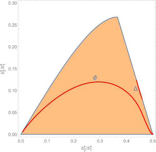
Figure 7: ${\mathcal{B}}_{{\rm{II}}}$: Region of existence of the type-II Riemann ellipsoids. The red lines $\Phi$ and $\Delta$ correspond to saddle-centre bifurcations

We select the ellipsoid with $(S^{2}_{L}\times S^{2}_{R})$-coordinates $(\mu^{+}_{N}(b_{1}^{\ast},b_{3}^{\ast},b_{2}^{\ast}),$ $\mu^{-}_{N}(b_{3}^{\ast},b_{1}^{\ast},b_{2}^{\ast}))$. The analysis for its adjoint essentially follows suit. Now $L$, $R$ are related to $b^{\ast}$ by

$$\begin{array}[]{rcl}L&=&\sqrt{N^{R}_{+}(b_{1}^{\ast},b_{3}^{\ast},b_{2}^{\ast})^{2}+N^{R}_{-}(b_{3}^{\ast},b_{1}^{\ast},b_{2}^{\ast})^{2}},\\[5.59721pt] R&=&\sqrt{N^{R}_{-}(b_{1}^{\ast},b_{3}^{\ast},b_{2}^{\ast})^{2}+N^{R}_{+}(b_{3}^{\ast},b_{1}^{\ast},b_{2}^{\ast})^{2}}.\\ \end{array}\\$$

The symplectic transformation suited for this case is

$$\begin{array}[]{lcl}b_{i}&=&b_{i}^{\ast}+{\bar{b}_{i}},\quad c_{i}={\bar{c}_{i}},\\[4.30554pt] m_{1}&=&-q_{1}\sqrt{L-\frac{q_{1}^{2}+p_{1}^{2}}{4}},\quad m_{2}=L-\frac{q_{1}^{2}+p_{1}^{2}}{2},\quad m_{3}=p_{1}\sqrt{L-\frac{q_{1}^{2}+p_{1}^{2}}{4}},\\[4.30554pt] m_{4}&=&-q_{2}\sqrt{R-\frac{q_{2}^{2}+p_{2}^{2}}{4}},\quad m_{5}=R-\frac{q_{2}^{2}+p_{2}^{2}}{2},\quad m_{6}=p_{2}\sqrt{R-\frac{q_{2}^{2}+p_{2}^{2}}{4}},\end{array}$$ (22)

with

$$q_{i}=q_{i}^{\ast}+\bar{q}_{i},\quad p_{i}=p_{i}^{\ast}+\bar{p}_{i},$$

and such that

$$\begin{array}[]{lcllcl}L&=&\frac{1}{2}(p_{1}^{\ast 2}+q_{1}^{\ast 2}),&R&=&\frac{1}{2}(p_{2}^{\ast 2}+q_{2}^{\ast 2}),\\[6.45831pt] q_{1}^{\ast}&=&\frac{-\sqrt{2}\,m_{1}^{\ast}}{(m_{1}^{\ast 2}+m_{3}^{\ast 2})^{1/4}},&q_{2}^{\ast}&=&\frac{-\sqrt{2}\,m_{4}^{\ast}}{(m_{4}^{\ast 2}+m_{6}^{\ast 2})^{1/4}},\\[6.45831pt] p_{1}^{\ast}&=&\frac{\sqrt{2}\,m_{3}^{\ast}}{(m_{1}^{\ast 2}+m_{3}^{\ast 2})^{1/4}},&p_{2}^{\ast}&=&\frac{\sqrt{2}\,m_{6}^{\ast}}{(m_{4}^{\ast 2}+m_{6}^{\ast 2})^{1/4}}.\\ \end{array}$$

We notice that the specific values of $L$, $R$, $q_{i}^{\ast}$, $p_{i}^{\ast}$, $m_{i}^{\ast}$ are related to each other through the previous formulae. All of them are ultimately explicitly written as functions of the parameters $b^{\ast}$.

By picking some samples in the region of the parametric plane denoted by ${\mathcal{B}}_{\rm II}$, we have numerically determined that the unstable ellipsoids of type II have either focus $\times$ focus or centre $\times$ centre $\times$ focus linearisation in the upper part of their region of existence. At some point, the focus $\times$ focus equilibria changes to linearisation of type centre $\times$ centre $\times$ focus. Eventually, a Hamiltonian-Hopf bifurcation occurs and they become linearly stable (centre $\times$ centre $\times$ centre $\times$ centre) with two positive signs in front of the $\omega_{i}>0$ and two negative ones.

On the boundary line $b_{1}^{\ast}=2\,b_{2}^{\ast}+b_{3}^{\ast}$ the equilibria are unstable of focus $\times$ saddle $\times$ saddle or centre $\times$ centre $\times$ centre $\times$ saddle type. At some point they become linearly stable with linearisation of centre $\times$ centre $\times$ centre $\times$ centre type, the quadratic normal-form Hamiltonian being indefinite with with two positive signs in front of the $\omega_{i}>0$ and two negative ones. They are linearly stable in a very narrow strip and then change stability to become unstable with linearisation centre $\times$ centre $\times$ centre $\times$ saddle. This change is in correspondence with a saddle-centre bifurcation, as we shall show with detail in Theorem 7.1. This exploration is compatible with the findings in fasso2001stability, although Fassò and Lewis refer to spectral stability, it is indeed linear stability, which is a bit stronger.

It is likely that there are two kinds of bifurcations involving type-II ellipsoids: on the one hand, Hamiltonian-Hopf bifurcations, where a linearly-stable equilibrium loses its stable character and two of the four pure imaginary eigenvalues change to become a quadruplet of complex eigenvalues. On the other hand, saddle-centre bifurcations, where a pair of pure imaginary eigenvalues becomes real. To prove that such a bifurcation takes place one has to compute higher-order terms because a mere linear analysis is not enough, as we show in Theorem 7.1 below. Besides, there is a transition line between focus $\times$ focus to centre $\times$ centre $\times$ focus regime, but we do not pay attention to it.

In Fig. 7 we represent in red the curves corresponding to the saddle-centre bifurcations. Here we do not plot the Hamiltonian-Hopf bifurcations because we leave the study of this bifurcation for type-III ellipsoids. They can be seen in Fig. 4 of fasso2001stability. An interesting degenerate case is the point in parametric plane where the Hamiltonian-Hopf and the saddle-centre bifurcations meet.

Now we focus on the quasi-periodic saddle-centre bifurcation. We follow the ideas of BroerHuitemaSevryuk; HanssmannCentreSaddle, adapting them to our setting. The main result of the section is given next.

Theorem 7.1.

Type-II ellipsoids undergo a quasi-periodic saddle-centre bifurcation. Additionally there is a degenerate case corresponding to a tangency between two curves, one regarding a saddle-centre bifurcation and the other one regarding a Hamiltonian-Hopf bifurcation.

Proof: We begin our proof in a similar way as we initiated the proof of Theorem 6.2. We introduce two rotation matrices ${\mathcal{R}}(\gamma_{1})$ and ${\mathcal{R}}(\gamma_{2})$ to construct a symplectic transformation that allows us to get a simpler expression of the quadratic Hamiltonian in normal form.

Combining the initial change of coordinates (22) with the two rotation matrices we obtain the symplectic change

$$\begin{array}[]{lcl}m_{1}&=&-q_{1}\sqrt{L-\frac{q_{1}^{2}+p_{1}^{2}}{4}}\cos\gamma_{1}+p_{1}\sqrt{L-\frac{q_{1}^{2}+p_{1}^{2}}{4}}\sin\gamma_{1},\quad m_{2}=L-\frac{q_{1}^{2}+p_{1}^{2}}{2},\\[7.3194pt] m_{3}&=&p_{1}\sqrt{L-\frac{q_{1}^{2}+p_{1}^{2}}{4}}\cos\gamma_{1}+q_{1}\sqrt{L-\frac{q_{1}^{2}+p_{1}^{2}}{4}}\sin\gamma_{1},\\[7.3194pt] m_{4}&=&-q_{2}\sqrt{R-\frac{q_{2}^{2}+p_{2}^{2}}{4}}\cos\gamma_{2}+p_{2}\sqrt{R-\frac{q_{2}^{2}+p_{2}^{2}}{4}}\sin\gamma_{2},\quad m_{5}=R-\frac{q_{2}^{2}+p_{2}^{2}}{2},\\[7.3194pt] m_{6}&=&p_{2}\sqrt{R-\frac{q_{2}^{2}+p_{2}^{2}}{4}}\cos\gamma_{2}+q_{2}\sqrt{R-\frac{q_{2}^{2}+p_{2}^{2}}{4}}\sin\gamma_{2}.\end{array}$$

The angles $\gamma_{i}$ are introduced with the goal of getting some zero entries in the linearisation matrix that we are going to build.

The relations at the equilibrium are

$$\begin{array}[]{lcllcl}q_{1}^{\ast}&=&\displaystyle\frac{\sqrt{2}(-m_{1}^{\ast}\cos\gamma_{1}+m_{3}^{\ast}\sin\gamma_{1})}{(m_{1}^{\ast 2}+m_{3}^{\ast 2})^{1/4}},&p_{1}^{\ast}&=&\displaystyle\frac{\sqrt{2}(m_{3}^{\ast}\cos\gamma_{1}+m_{1}^{\ast}\sin\gamma_{1})}{(m_{1}^{\ast 2}+m_{3}^{\ast 2})^{1/4}},\\[8.61108pt] q_{2}^{\ast}&=&\displaystyle\frac{\sqrt{2}(-m_{4}^{\ast}\cos\gamma_{2}+m_{6}^{\ast}\sin\gamma_{2})}{(m_{4}^{\ast 2}+m_{6}^{\ast 2})^{1/4}},&p_{2}^{\ast}&=&\displaystyle\frac{\sqrt{2}(m_{6}^{\ast}\cos\gamma_{2}+m_{4}^{\ast}\sin\gamma_{2})}{(m_{4}^{\ast 2}+m_{6}^{\ast 2})^{1/4}}.\end{array}$$

We select $\gamma_{1}$ and $\gamma_{2}$ so that the terms of the transformed quadratic Hamiltonian containing $\bar{b}_{1}\bar{p}_{1},\bar{b}_{2}\bar{p}_{2},\bar{b}_{1}\bar{p}_{2},\bar{b}_{2}\bar{p}_{1}$ are zero. We end up with

$$\gamma_{1}=\arccos\left(\frac{m^{\ast}_{3}}{\sqrt{m_{1}^{\ast 2}+m_{3}^{\ast 2}}}\right),\quad\gamma_{2}=-\arccos\left(\frac{m^{\ast}_{6}}{\sqrt{m_{4}^{\ast 2}+m_{6}^{\ast 2}}}\right).\\$$

Next, we apply Markeev’s procedure (see Appendix LABEL:Linearization) to obtain the corresponding diagonal linear normal form in rectangular coordinates, say $z$. The linearisation matrix is

$${\mathcal{L}}=\left(\begin{array}[]{cccccccc}0&0&0&0&\ell_{1,5}&\ell_{1,6}&0&0\\ \vskip 6.0pt plus 2.0pt minus 2.0pt\cr 0&0&0&0&\ell_{1,6}&\ell_{2,6}&0&0\\ \vskip 6.0pt plus 2.0pt minus 2.0pt\cr 0&0&0&0&0&0&\ell_{3,7}&\ell_{3,8}\\ \vskip 6.0pt plus 2.0pt minus 2.0pt\cr 0&0&0&0&0&0&\ell_{3,8}&\ell_{4,8}\\ \vskip 6.0pt plus 2.0pt minus 2.0pt\cr\ell_{5,1}&\ell_{5,2}&\ell_{5,3}&\ell_{5,4}&0&0&0&0\\ \vskip 6.0pt plus 2.0pt minus 2.0pt\cr\ell_{5,2}&\ell_{6,2}&\ell_{6,3}&\ell_{6,4}&0&0&0&0\\ \vskip 6.0pt plus 2.0pt minus 2.0pt\cr\ell_{5,3}&\ell_{6,3}&\ell_{7,3}&\ell_{7,4}&0&0&0&0\\ \vskip 6.0pt plus 2.0pt minus 2.0pt\cr\ell_{5,4}&\ell_{6,4}&\ell_{7,4}&\ell_{8,4}&0&0&0&0\end{array}\right),$$

where the coefficients $\ell_{i,j}$ are given in terms of $b^{\ast}$. The relationship between both kinds of parameters is much more involved than in case of $S$-ellipsoids. Nevertheless, it has to be expected since the linearisation matrix has less zero blocks than the ones appearing in Appendix LABEL:Linearization. Anyway, we have succeeded in obtaining closed formulae and they are supplied in the Mathematica file. The expressions of the $\omega_{i}$ in terms of $\ell_{i,j}$ are also cumbersome but they can be computed explicitly. The reason is that they are obtained from the roots of the characteristic equation of an $(8\times 8)$-matrix, but this equation contains only even powers in the unknown, say $\lambda$. Thus, it is indeed a polynomial equation of degree four whose roots are derived in closed form. We have achieved this, arriving at formulae of quite big sizes but still manageable to work with them. The related eigenvectors are also provided. The values of $\omega_{i}$ as functions of $\ell_{i,j}$ are also presented in the Mathematica file.

As in the previous cases we apply the procedure due to Markeev and delineated in Appendix LABEL:Linearization. A last step is needed to make the approach valid when the frequency $\omega_{4}$ vanishes. We set $x_{4}\rightarrow\sqrt{\omega_{4}}x_{4}$, $y_{4}\rightarrow y_{4}/\sqrt{\omega_{4}}$, exactly as we did for the $S_{2}$-ellipsoids in the co-parallel regime. We arrive at the quadratic Hamiltonian function in normal form:

$$H_{2}(z)=-\frac{\omega_{1}}{2}(x_{1}^{2}+y_{1}^{2})+\frac{\omega_{2}}{2}(x_{2}^{2}+y_{2}^{2})+\frac{\omega_{3}}{2}(x_{3}^{2}+y_{3}^{2})-\frac{1}{2}(\omega_{4}^{2}x_{4}^{2}+y_{4}^{2}),$$

with $\omega_{i}>0$, $i=1,2,3$, while $\omega_{4}$ can be positive, zero or pure imaginary such that $\omega_{4}=\imath\bar{\omega}_{4}$ with $\bar{\omega}_{4}<0$. The corresponding transformation matrix $\mathcal{T}$, the one in charge of bringing $H_{2}$ to normal form, is symplectic and has real entries for $\omega_{4}\geq 0$ or pure imaginary. Moreover, $\mathcal{T}$ depends smoothly on $\omega_{4}$, thus it is a versal normal form. Up to this step the form of the quadratic Hamiltonian in normal form is the same as the one occurring in the co-parallel regime of the $S_{2}$-ellipsoids, excepting one sign. However the bifurcation is going to be different, but this will be concluded after analysing the higher-order terms.

As we have seen, the responsible for the bifurcation is the frequency $\omega_{4}$. Expressing $\omega_{4}$ as an explicit function of $b_{2}^{\ast}/b_{1}^{\ast}$ and $b_{3}^{\ast}/b_{1}^{\ast}$ is hard. Nevertheless, taking into account that the determinant of the linearisation matrix ${\mathcal{L}}$ is equal to the product of its eigenvalues, so $|{\mathcal{L}}|=(\omega_{1}\omega_{2}\omega_{3}\omega_{4})^{2}$. Then $\omega_{4}=0$ implies $|{\mathcal{L}}|=0$. This fact allows us to determine an analytical expression of the bifurcation curves subsequent to removing spurious terms. The relevant factor corresponding to the bifurcation lines in the parametric plot is given by a compact formula, and is provided in the Mathematica file. It has been depicted in Fig. 7 (red lines $\Phi$ and $\Delta$). Bifurcation line $\Phi$ corresponds to the lower arch in region ${\mathcal{B}}_{\rm II}$ in fasso2001stability (see Fig. 4 (b), (c) and (d)). Line $\Delta$ also appears in Fig. 4 (d) of fasso2001stability, although it requires some clarification that we do below.

After applying the linear transformation obtained above to terms of degree three and four we apply a Lie transformation Deprit to compute the corresponding normal form up to terms of degree four in rectangular coordinates. We want to see that the requested non-degeneracy conditions needed to prove that a quasi-periodic saddle-centre bifurcation takes place are fulfilled. To achieve this, we pass to complex variables by means of the change (14).

The linear normal form in complex/real variables, that is, in $Z$ defined for the $S_{2}$-ellipsoids, has as Hamiltonian function

$$H_{2}(Z)=-\imath\omega_{1}X_{1}Y_{1}+\imath\omega_{2}X_{2}Y_{2}+\imath\omega_{3}X_{3}Y_{3}-\mbox{$\frac{1}{2}$}(\omega_{4}^{2}X_{4}^{2}+Y_{4}^{2}).\\$$

Due to the structure of the zeroth-order Hamiltonian $H_{2}$ and taking into account that due to the lack symmetries if compared to $S_{2}$-ellipsoids, some terms of degree three have to be retained in the transformed Hamiltonian, we impose the first-order normal-form Hamiltonian, which is composed by homogeneous polynomials of degree three in complex/real coordinates, to be of the form

$$H_{3}(Z)={\mathsf{C}}_{1}X_{1}Y_{1}X_{4}+{\mathsf{C}}_{2}X_{2}Y_{2}X_{4}+{\mathsf{C}}_{3}X_{3}Y_{3}X_{4}+{\mathsf{C}}_{4}X_{4}^{3},$$

with ${\mathsf{C}}_{i}$ some parameters (real or complex) that have to be determined. Notice that we use the same name for the transformed and untransformed coordinates. The reason for the monomials chosen to get $H_{3}$ is due to the form $H_{2}$ has and in particular due to the nilpotent part of $H_{2}$ for $\omega_{4}=0$. The same will happen for higher-order terms. Introducing the generating function $\mathcal{W}_{1}$ as a homogeneous polynomial in $Z$ of degree three with undetermined coefficients, we impose that the related homological equation be satisfied. This leads to a system of linear equations whose unknowns are the coefficients of $\mathcal{W}_{1}$ and the ${\mathsf{C}}_{i}$. This is an underdetermined system with 120 linear equations and 124 unknowns that has been solved. Coefficients ${\mathsf{C}}_{i}$ depend explicitly on the $\ell_{i,j}$, $\omega_{i}$ and $b^{\ast}$.

Passing from the $X_{i}/Y_{i}$ to the actions $I_{i}$, $i=1,2,3$, the truncated normal-form Hamiltonian at first order, that is, $H_{2}+H_{3}$ reads as

$$\begin{array}[]{lcl}H^{3}(I,X_{4},Y_{4})&=&-\omega_{1}I_{1}+\omega_{2}I_{2}+\omega_{3}I_{3}-\mbox{$\frac{1}{2}$}(\omega_{4}^{2}X_{4}^{2}+Y_{4}^{2})\\[4.30554pt] &&-\,\imath({\mathsf{C}}_{1}I_{1}+{\mathsf{C}}_{2}I_{2}+{\mathsf{C}}_{3}I_{3})X_{4}+{\mathsf{C}}_{4}X_{4}^{3}.\end{array}$$

In the process of getting the suitable normal form for the saddle-centre bifurcation we make a shift in $X_{4}$

$$X_{4}=\bar{X}_{4}+X_{40},\quad Y_{4}=\bar{Y}_{4},$$

where

$$X_{40}=\frac{\omega_{4}^{2}}{6{\mathsf{C}}_{4}}$$

and apply it to $H^{3}$. In this way we absorb the term in $\bar{X}_{4}^{2}$, providing the denominator of $X_{40}$ does not vanish at the bifurcation curve, that is, ${\mathsf{C}}_{4}\neq 0$, arriving at a suitable pattern for proving the existence of a saddle-centre bifurcation. We get

$$H^{3}(I,\bar{X}_{4},\bar{Y}_{4})=-\omega_{1}I_{1}+\omega_{2}I_{2}+\omega_{3}I_{3}-\mbox{$\frac{1}{2}$}\bar{Y}_{4}^{2}+{\mathsf{C}}_{5}(I)+{\mathsf{C}}_{6}(I)\bar{X}_{4}+{\mathsf{C}}_{4}\bar{X}_{4}^{3},$$

where ${\mathsf{C}}_{5}$ and ${\mathsf{C}}_{6}$ depend linearly on the actions and on the parameters of the problem.

In a bid to get the persistence of KAM tori associated to the bifurcation, the normal form $H^{3}$ is still too degenerate and the related Hessian that we have to check is zero. For this reason we have to compute the order two (second step of the normal form procedure) in order to incorporate a quadratic dependence in the actions and obtain the required rank (three) to prove this persistence.

The second-order normal form, i.e. the terms of degree four in complex/real variables $Z$, is of the form

$$\begin{array}[]{lcl}H_{4}(Z)&=&Q_{1}(X_{1}Y_{1})^{2}+Q_{2}(X_{2}Y_{2})^{2}+Q_{3}(X_{3}Y_{3})^{2}+Q_{4}X_{4}^{4}+Q_{5}X_{1}Y_{1}X_{2}Y_{2}\\[4.30554pt] &&+\,Q_{6}X_{1}Y_{1}X_{3}Y_{3}+Q_{7}X_{2}Y_{2}X_{3}Y_{3}+Q_{8}X_{1}Y_{1}X_{4}^{2}+Q_{9}X_{2}Y_{2}X_{4}^{2}\\[4.30554pt] &&+\,Q_{10}X_{3}Y_{3}X_{4}^{2},\end{array}$$

where the $Q_{i}$ coefficients are determined, together with the ones of the generating function ${\mathcal{W}}_{2}$. This is achieved by solving a linear system of 330 equations and 340 unknowns. After some simplifications and arrangements done with the aim of controlling that the denominators of the monomials forming the generating function do not vanish when $\omega_{4}=0$, we have ended up with concrete expressions for $Q_{i}$ and ${\mathcal{W}}_{2}$, which in turn are explicit functions of $b^{\ast}$.

Now we consider the truncated normal form at degree four in the (transformed) coordinates $I$, $X_{4}$, $Y_{4}$. Hamiltonian $H^{4}=H_{2}+H_{3}+\frac{1}{2}H_{4}$ reads as

$$H^{4}(I,X_{4},Y_{4})=F_{1}(I)-\mbox{$\frac{1}{2}$}Y_{4}^{2}+F_{2}(I)X_{4}+F_{3}(I)X_{4}^{2}+F_{4}X_{4}^{3}+F_{5}X_{4}^{4},$$

with $F_{i}(I)$, $i=1,2,3$, polynomials in $I$ that depend on $b^{\ast}$ whereas $F_{4}$, $F_{5}$ are functions of $b^{\ast}$. Specifically

$$\begin{array}[]{rcl}F_{1}(I)&=&-\omega_{1}I_{1}+\omega_{2}I_{2}+\omega_{3}I_{3}\\[3.44444pt] &&-\,\mbox{$\frac{1}{2}$}(Q_{1}I_{1}^{2}+Q_{2}I_{2}^{2}+Q_{3}I_{3}^{2}+Q_{5}I_{1}I_{2}-Q_{6}I_{1}I_{3}+Q_{7}I_{2}I_{3}),\\[4.30554pt] F_{2}(I)&=&-\imath({\mathsf{C}}_{1}I_{1}+{\mathsf{C}}_{2}I_{2}+{\mathsf{C}}_{3}I_{3}),\\[4.30554pt] F_{3}(I)&=&-\mbox{$\frac{1}{2}$}\omega_{4}^{2}-\mbox{$\frac{\imath}{2}$}(Q_{8}I_{1}+Q_{9}I_{2}+Q_{10}I_{3}),\\[4.30554pt] F_{4}&=&{\mathsf{C}}_{4},\\[4.30554pt] F_{5}&=&\mbox{$\frac{1}{2}$}Q_{4}.\end{array}$$

Hamiltonian $H_{3}$ is taken above without doing the shift.

We can eliminate the term depending on $X_{4}^{2}$ as before, but this time it is a bit more involved. Calling $\psi_{i}$ the angles conjugate to $I_{i}$ we introduce the transformation

$$\begin{array}[]{rcl}X_{4}&=&\bar{X}_{4}+X^{\ast}_{40}(\bar{I}),\quad Y_{4}=\bar{Y}_{4},\\[4.30554pt] \psi_{i}&=&\displaystyle\bar{\psi}_{i}+\bar{Y}_{4}\frac{\partial{X^{\ast}_{40}(\bar{I})}}{\partial\bar{I}_{i}},\quad I_{i}=\bar{I}_{i}.\end{array}$$

The modification done on $\psi_{i}$ is due to the fact that $X^{\ast}_{40}$ depends on the $\bar{I}$. Then, the change is symplectic. An additional detail is that when we solve the equation for determining $X^{\ast}_{40}$, there are two possible solutions (it is obtained by solving a second-degree equation) and the right choice depends on the sign of the coefficient of $X_{4}^{3}$ in the Taylor expansion for the specific values of $b^{\ast}$. We remark that $X^{\ast}_{40}(0)=0$ when $\omega_{4}=0$.

The resulting (truncated) normal-form Hamiltonian becomes

$$H^{4}(\bar{I},\bar{X}_{4},\bar{Y}_{4})=F^{\ast}_{1}(\bar{I})-\mbox{$\frac{1}{2}$}\bar{Y}_{4}^{2}+F^{\ast}_{2}(\bar{I})\bar{X}_{4}+F^{\ast}_{4}(\bar{I})\bar{X}_{4}^{3}+F_{5}\bar{X}_{4}^{4},$$

with $F^{\ast}_{1}$, $F^{\ast}_{2}$, $F^{\ast}_{4}$ functions of $\bar{I}$. The term $F_{5}\bar{X}_{4}^{4}$ can be considered of higher order for $\bar{X}_{4}$ small enough.

At this point we examine the possible resonances introduced in the Lie transformation process. More precisely we have checked whether the denominators of the terms of the generating functions vanish when $\omega_{4}=0$. Focusing on the line $\Phi$, being the approach the same for $\Delta$, we have found three fourth-order resonances, namely

$$-\omega_{1}+3\,\omega_{3},\quad-2\,\omega_{1}+\omega_{2}+\omega_{3},\quad\omega_{1}-\omega_{2}+2\,\omega_{3}.$$

These values are removed from our study and are represented in Fig. 8. Concretely, we have to discard from the parametric plane the points $(b_{2}^{\ast}/b_{1}^{\ast},b_{3}^{\ast}/b_{1}^{\ast})$ such that the linear combinations of the frequencies given above become zero. We obtain: $-\omega_{1}+3\,\omega_{3}=0$ for $b_{2}^{\ast}/b_{1}^{\ast}\approx 0.144,0.272,0.438$; $-2\,\omega_{1}+\omega_{2}+\omega_{3}=0$ for $b_{2}^{\ast}/b_{1}^{\ast}\approx 0.240,0.468,0.485$; $\omega_{1}-\omega_{2}+2\,\omega_{3}=0$ for $b_{2}^{\ast}/b_{1}^{\ast}\approx 0.177,0349,0.379$. The corresponding values of $b_{3}^{\ast}/b_{1}^{\ast}$ are obtained after solving $\omega_{4}=0$. By a continuity argument we also remove small neighbourhoods of these points, because some denominators of the formulae become very small. These roots and their neighbourhoods have to be discarded from our analysis.

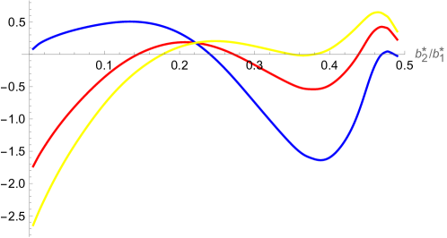
Figure 8: Resonances appearing in the computation of the normal form to determine the quasi-periodic saddle-centre bifurcation for type-II ellipsoids. The red line corresponds to $-\omega_{1}+3\,\omega_{3}$, the blue one to $-2\,\omega_{1}+\omega_{2}+\omega_{3}$ and the yellow one to $\omega_{1}-\omega_{2}+2\,\omega_{3}$

We deal now with the conditions that $H^{4}$ has to fulfill in a bid to establish the occurrence of the saddle-centre bifurcation. We apply Theorem 4.4 of hanssmann2006local. We need to study the behaviour of $F^{\ast}_{2}$ and $F^{\ast}_{4}$, respective coefficients of $\bar{X}_{4}$ and $\bar{X}_{4}^{3}$. In particular we have to prove that $F^{\ast}_{2}$ vanishes for $\bar{I}=0$, $\omega_{4}=0$ but $F^{\ast}_{4}(0)\neq 0$ for $\omega_{4}=0$. On the one hand, as for $\omega_{4}=\bar{I}=0$ we know that the coefficient $X^{\ast}_{40}$ vanishes, one has that $F^{\ast}_{2}(0)=F_{2}(0)=0$. On the other hand we observe that the coefficient $F^{\ast}_{4}(0)$ (with $\omega_{4}=0$) is equal to the coefficient ${\mathsf{C}}_{4}$, which is given in an explicit way on the bifurcation line $\Phi$ in terms of $b^{\ast}$ and placed in the Mathematica file. However, in a bid to check that it does not vanish on the line $\Phi$ we need to proceed numerically though with very high precision in the computations. Thus, we check how it evolves along the bifurcation curve $\Phi$. We depict in Fig. 9 the variation of this coefficient when $b^{\ast}$ is in $\Phi$.

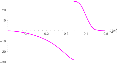
Figure 9: Coefficient ${\mathsf{C}}_{4}$ with $\omega_{4}=0$ evaluated along the line $\Phi$. It never touches the horizontal axis. In fact, when $b_{2}^{\ast}/b_{1}^{\ast}\approx 0$, the coefficient is $-0.0078$ and it goes on decreasing up to the point $b_{2}^{\ast}/b_{1}^{\ast}\approx 0.3381$ where a discontinuity occurs. Its corresponding $b_{3}^{\ast}/b_{1}^{\ast}$ jumps from approximately $-27.9366$ to $27.9366$. Then ${\mathsf{C}}_{4}$ becomes positive and remains above the horizontal axis. When $b_{2}^{\ast}/b_{1}^{\ast}\approx 1/2$, ${\mathsf{C}}_{4}$ takes its minimum value, $0.0038$

The values of $b^{\ast}$ related to the resonances presented above and small balls around them are not taken into account for our analysis. The value $b_{2}^{\ast}/b_{1}^{\ast}\approx 0.3381$ (see Fig. 9) has nothing to do with the resonances. In fact, it is related to the manner the linear normal form has been built. In spite of that, the linear change is properly defined for this value. The corresponding ratio $b_{3}^{\ast}/b_{1}^{\ast}$ (obtained imposing that the point $b^{\ast}$ belongs to $\Phi$) is approximately $0.1163$ though it does not affect the overall study since this coefficient does not vanish along the bifurcation curve.

In a final step we prove the persistence of the KAM tori related to the bifurcation. We introduce

$$\tilde{c}(I)=F^{\ast}_{2}(\bar{I}),\quad\tilde{\omega}_{i}(I)=\displaystyle\frac{\partial F^{\ast}_{1}(\bar{I})}{\partial\bar{I}_{i}},$$

and define the map

$$\xi:\bar{I}\rightarrow\left(\tilde{c}(\bar{I}),\tilde{\omega}_{1}(\bar{I}),\tilde{\omega}_{2}(\bar{I}),\tilde{\omega}_{3}(\bar{I})\right).$$

We prove that it is a submersion at $\omega_{4}=0$, i.e. that $\xi$ is differentiable with its differential being surjective everywhere. We get $D\tilde{c}(0)=-\imath({\mathsf{C}}_{1},{\mathsf{C}}_{2},{\mathsf{C}}_{3})\neq(0,0,0)$ along the curve $\Phi$, where we have discarded the resonance values but not the point $(b_{2}^{\ast}/b_{1}^{\ast},b_{3}^{\ast}/b_{1}^{\ast})\approx(0.3381,0.1163)$. More precisely, evaluating ere the norm of $D\tilde{c}(0)$ along the bifurcation curve we have noticed that it is always positive, and tends to zero when approaching the right-end point of the curve, where it takes its minimum value, around $0.0089$. Analogously to the analysis made in Section 4 we form the ($3\times 3$)-matrix $\mathtt{M}$ where its first row is $(\tilde{\omega}_{1}(\bar{I}),\tilde{\omega}_{2}(\bar{I}),\tilde{\omega}_{3}(\bar{I}))$, its second row is the partial derivative of the first one with respect to $\bar{I}_{1}$ and its third row is the partial derivative with respect to $\bar{I}_{2}$. The determinant of $\mathtt{M}$ evaluated at $\bar{I}=\omega_{4}=0$ is different from zero along the bifurcation curve $\Phi$, excepting a discrete set of points which have nothing to do with the resonances dealt with above. For those points where $\text{ M }\text{ = 0}weformthematricesbutinsteadofderivingwithrespectto\text{I\_1}\text{,}\text{I\_2},wedoitwithrespectto\text{I\_1}\text{,}\text{I\_3}orto\text{I\_1}\text{,}\text{I\_2}.Wehavecheckedthatatleastoneofthesetwodeterminantsdoesnotvanishonthepointswhere\text{M}issingular,soweconcludethattherankof\text{M}(orofoneoftheotherpossiblesmatrices)isthree.Ofcourse,thevaluesalreadyremovedwheretheanalysiscannotbeapplied.Hence,itisconcludedthatthemapintroducedaboveisasubmersion.Thecalculationsaregiveninthe\mathrm{Mathematica}file.Thisallowsustoconcludethepersistenceoftheinvarianttorithatinterplayinthebifurcation.Asthesignof\overline{\text{Y}}\text{\_4^2}in\text{H^4}isalwaysnegative,theKAMtoriarisewhentheproduct\text{F\_2^∗(}\overline{\text{I}}\text{) F\_4^∗( }\overline{\text{I}}\text{)}isnegative.Actually,thisproductisafunctionwithnon-trivialdependenceon\overline{\text{I}},asitcontainsrationaltermsandsquareroots,henceitcantakepositive,negativeorcomplexvalues,accordingtotherelativevaluesamongthe\overline{\text{I}}\text{\_i}.Thus,when\text{F\_2^∗(}\overline{\text{I}}\text{) F\_4^∗( }\overline{\text{I}}\text{) ¡ 0}thereisafamilyofelliptic\text{3}-toriandanotheroneofhyperbolictypeanddimension\text{2}.Thesetwofamiliesmergetobecomeoneonthebifurcationcurve\text{Φ}.Then,\text{F\_2^∗( }\overline{\text{I}}\text{) = 0}andtheresultingtoribecomeparabolic.Thetoridisappearwhen\text{F\_2^∗( }\overline{\text{I}}\text{) F\_4^∗( }\overline{\text{I}}\text{) ¿ 0}.Theparabolic\text{3}-torialsopersistunderperturbation.Toconcludetheproofofthetheoremwehavetoanalysethepointintheparametricplanewheretwotypesofbifurcationstakeplace.Thecorrespondingnormal-formHamiltonianhasbeenalsoobtainedanalytically.ThistangencypointappearsinFig.\text{<span class="ltx\_ref ltx\_missing\_label ltx\_font\_italic ltx\_ref\_self">LABEL:fig:Degenerate</span>}.WehavedeferredthestudyofoneoftheHamiltonian-HopfbifurcationsthattakeplaceinthecasesofellipsoidsoftypesI,IIandIIItothenextsection.HereweonlyshowhowthetwobifurcationsareexperiencedbytheRiemannellipsoidsinasinglepointoftheparametricplane.Thisisindeedtheonlypointwherewehaveobservedtwobifurcations.\text{Figure 10Figure 1010Figure 1010TangencypointbetweentheHamiltonian-Hopfbif}$