Influence of HW-SW-Co-Design
on Quantum Computing Scalability

Abstract

The use of quantum processing units (QPUs) promises speed-ups for solving computational problems. Yet, current devices are limited by the number of qubits and suffer from significant imperfections, which prevents achieving quantum advantage. To step towards practical utility, one approach is to apply hardware-software co-design methods. This can involve tailoring problem formulations and algorithms to the quantum execution environment, but also entails the possibility of adapting physical properties of the QPU to specific applications. In this work, we follow the latter path, and investigate how key figures—circuit depth and gate count—required to solve four cornerstone NP-complete problems vary with tailored hardware properties.

Our results reveal that achieving near-optimal performance and properties does not necessarily require optimal quantum hardware, but can be satisfied with much simpler structures that can potentially be realised for many hardware approaches. Using statistical analysis techniques, we additionally identify an underlying general model that applies to all subject problems. This suggests that our results may be universally applicable to other algorithms and problem domains, and tailored QPUs can find utility outside their initially envisaged problem domains. The substantial possible improvements nonetheless highlight the importance of QPU tailoring to progress towards practical deployment and scalability of quantum software.

I Introduction

NP-Complete problems are of great interest in computer science and mathematics, as many industrial problems belong to this complexity class. They are believed to be computationally intractable for classical computers, at least in the worst case. This means that for large instances of these problems, it may not be possible to find a solution in a reasonable amount of time using any known algorithm. Industrial use-cases already benefit from approximating optimisation. These problems can be rewritten as NP-optimisation (NPO) problems and also include combinatorial elements to represent each problem [1, 2]. In practice, there exist heuristics and approximation algorithms that can be used to find good near-optimal solutions to some NP-complete problems by choosing a trade-off between performance and result quality, albeit it is known that problems exist that defy such techniques [3, 4].

Quantum algorithms in general have the potential to improve both, the quality and performance of approximate solutions to NP-complete problems [5]. QAOA (Quantum Approximate Optimisation Algorithm) is a particularly well-known and widely studied quantum algorithm for finding approximate solutions to combinatorial optimisation problems. However, among other factors, current quantum hardware limitations restrict the potential of using QAOA to solve problems of practical interest. Quantum computers face different challenges; for instance they are limited to a relatively small number of qubits, typically ranging from around 50 to 400. Scaling quantum computers to large numbers of qubits is a difficult engineering problem that also heavily depends on the specific hardware platform. Another problem is that quantum computers are susceptible to noise and distortions from their environment and suffer from imperfections in the control signals [6], both leading to errors in the operations performed on the qubits, and limited decoherence times.

Changes to the hardware architecture can influence the connectivity between qubits, the coherence time, and the gate error rates. These modifications impact the performance and resource requirements of quantum algorithms, such as the number of gates needed to execute the quantum circuit, the number of measurements required and the amount of memory and time needed to store and manipulate quantum states. In this paper, we consider the effects of such hardware improvements on four NP- complete problems: Travelling Salesperson (TSP), Number Partitioning (NumPart), Maximum Cut (MaxCut) and Maximum 3-Satisfiability (Max3Sat).

This is of particular importance in the current era of noisy, intermediate-scale quantum (NISQ) computers, which is expected to last for at least several years (possibly even decades) until fault-tolerant, perfect quantum computing becomes feasible. Yet, there is an increasing interest in utilising NISQ devices in high- performance computing (HPC) scenarios, and tailoring NISQ devices to problems is seen as a possible or even necessary of stepping towards practically relevant quantum speedups and advantage. As properties of quantum algorithms depend on QPU (hardware) properties [7], hardware-software co-design can help to address some of the key challenges of current quantum devices [8]. By designing algorithms and programs optimised for these limitations, it may be possible to surpass result quality of more generic approaches. It is also an important and promising approach to optimise the performance and efficiency of quantum computing systems by putting both the hardware and software component as a cohesive unit. The focus of this paper is to examine the impact of hardware-software co-design on quantum computing scalability. We use numerical experiments to explore the potential for co-design using a hybrid quantum algorithm (QAOA) applied so several subject problems. The quantum circuits are compiled to different types of simulated hardware backends, which are extended from the topology of the IBM-Q devices.

The paper is augmented by a reproduction package [9], which is available for download (link in PDF). Some supporting material that we could not present in the main text is available on the supplementary website.

The rest of this work is structured as follows. Section II reviews related work. Following in Sec. III, we explain the principles behind our approach, and also elaborate on properties of the subject problems. Results from numerical experiments, conducted in Sec. IV, are analysed in Sec. V, which also presents a general model that universally describes all subject problems. Finally, Sec. VII discusses the consequences of our findings, together with an outlook on future research directions.

II Related Work

QAOA has been studied as a promising approach to solve combinatorial optimisation problems. Several previous works have focused on optimising QAOA for available quantum hardware. The main challenges in this context are the limited number of qubits and the high error rates of current quantum devices. To address these challenges, different approaches have been proposed, such as the use of hardware-software co-design, error mitigation techniques [10], hardware-efficient ansätze [5] or hybrid classical-quantum optimisation [11]. Lotshaw et al. [12] discuss the impact of problem sizes and complexity on QAOA performance and resource requirements on contemporary hardware, and also analyse scalability of the algorithm under different hardware topologies. Furthermore, Wille et al. [13] address the challenge of mapping quantum circuits to the topology of targeted architectures and present a tool for tackling this problem. Some works have focused more on designing quantum hardware that is optimised for specific quantum algorithms. For example in the work of Kandala et al. [14], a superconducting quantum processor was optimised for the variational quantum eigensolver (VQE) algorithm. The paper shows that this approach can significantly reduce the number of gates required to implement VQE on the hardware. In [8], an architecture design-flow for superconducting quantum computers is proposed that finds a trade-off between optimisation of the processor’s yield rate and a mapping with minimal gate-overhead. The ansatz is compared to other designs using the example of VQE for quantum chemistry calculations. Furthermore, Linke et al. [15] assert that co-designing quantum applications for specific purposes is crucial to successfully utilise quantum computers in the near future. They reach this conclusion by comparing identical quantum algorithms on two different hardware platforms.

III Context and Foundations

In the following, we lay some foundations necessary to understand our approach and rationale behind the experiments..

III-A Quantum Optimisation with QAOA

QAOA is a widely used variational hybrid quantum algorithm on NISQ hardware developed by Fahri  et al. in 2014 [5]. The algorithm has shown promising results on small-scale quantum devices for several optimisation problems, including the MaxCut problem, TSP [16], or similar problems [17]. As quantum hardware continues to improve, QAOA and other quantum optimisation algorithms are expected to play an increasingly important role in solving real-world problems.

III-A1 Algorithm

QAOA produces approximate solutions for combinatorial optimisation problems, which are described by a problem Hamiltonian $H_{p}$. The algorithm consists of several layers of parameterised unitary operators $U(\beta,\gamma)$. As the number of layers $p\geq 1$, $p\in\mathbb{N}$ increases, the quality of the approximation improves [5]. First, the quantum register is initialised in a well-defined state and after applying the unitary operators, the expectation value of $H_{p}$ is measured in the final state. The parameters $\beta,\gamma$ of the quantum circuit are optimised by classical methods such that the expectation value of $H_{p}$ is minimised.

Each layer consists of two different kinds of unitaries, $U(\beta_{i})=e^{i\beta H_{B}}$ and $U(\gamma_{i})=e^{i\gamma H_{P}}$. The algorithm applies a mixer Hamiltonian, typically a Pauli-X operator, to each qubit using the $U(\beta_{i})=e^{i\beta H_{B}}$ unitary. This is followed by a combination of single qubit $Z-$rotations $R_{Z}(\gamma_{i})$ and two-qubit rotation gates $R_{ZZ}(\gamma_{i})$ composing the $U(\gamma_{i})=e^{i\gamma H_{P}}$ unitary. Multiple layers of this process correspond to a discretized time evolution governed by the Hamiltonians $H_{P}$ and $H_{B}$. The algorithm’s initial state is usually the ground state of $H_{B}$, prepared using Hadamard gates $H$. To optimise the objective function, the quantum circuit is executed multiple times, and the qubits are measured in the computational basis. The mean of the expectation values of $H_{P}$ for each measurement outcome is minimised by the classical optimiser, and the optimal solution is derived as the state or bit string with the lowest energy expectation value in the probability distribution obtained from the final set of parameters. The algorithm determines the minimum value of the objective function specified in quadratic unconstrained binary form (QUBO). A classical algorithm that can efficiently sample the output distribution of QAOA even for $p=1$, cannot exist based on reasonable complexity-theoretic assumptions. This indicates the possibility of quantum advantage, but practical utility on real-world problems require further investigations [7].

III-B Translation of algorithms to quantum hardware

When programming a quantum algorithm, initially no restrictions on the type of gates being used or the interaction between qubits is made. However, to execute a certain quantum algorithm on a specific hardware backend, it needs to be compiled [18] to the properties of the backend, which is also called transpilation [19]. The most important properties of a quantum computer that influence the transpilation of circuits are the size of the backend, that is, the number of qubits available, their geometric arrangement and connectivity, and the native gate set. For the actual execution of the circuit, also other factors such as the fidelities of gate operations, initialization and measurement as well as the decoherence and gate operation times play an important role.

The connectivity measures the number of other qubits one qubit can interact with, and thus the ability to perform a two-qubit gate operation between them. If a two-qubit gate needs to be executed between qubits which are not connected, a Swap gate can be applied to swap the states of two qubits. The geometric layout and connectivity of the QPU can be depicted by a graph with nodes representing the qubits and edges connecting two qubits if an interaction between them is possible. Analogously, the circuit that is executed can also be represented by a graph, which has an edge between two nodes, if a two-qubit gate is performed between the corresponding qubits. The transpilation process maps this circuit graph to the hardware graph, while taking into account further restrictions, such as the native gate set.

Due to the decomposition of gates into the native gate set of the hardware as well as the insertion and further decomposition of Swap gates, the transpiled circuit contains more gates in total. This is crucial in the current NISQ-era, as each gate introduces an error, and thus the quality of the results is expected to drop with a growing number of operations. Moreover, the circuit depth is increased, which measures the maximum length of the circuit accounting for parallel execution of gates, as well as the overall runtime of the algorithm, due to the finite execution time of each gate. The available quantum computers only have a limited decoherence time, in which operations can be performed, that should not be exceeded by the algorithm runtime.

Thus, to increase the performance of quantum algorithms on near-term quantum computers, the number of gate operations should be minimised. This could be achieved by designing optimised algorithms or by increasing the connectivity of the hardware.

The ability to modify these properties depends on the type of the QPU being used. Today, several different types of quantum computing hardware exist, which differ by the physical implementation of qubits. The two states $\ket{0}$ and $\ket{1}$ can be encoded in various different ways such as the naturally occurring discrete energy levels of single ions or atoms, the effective energies of superconducting circuit elements or in the spatial modes of single photons, to just name a few [20, 21, 22, 23]. Along with the choice of qubits, also the control and readout techniques, the infrastructure requirements (e.g., if cooling with a cryostat is needed) and the properties relevant for mapping between logical and physical circuits, such as the number of qubits, the native gate set and the connectivity are different for each type of QPU. This means that the performance of a quantum algorithm usually heavily depends on the type of hardware that it is running on.

III-C Problem selection

In this paper, we focus on problems that belong to complexity class NP-Complete (NPC), as it contains practically relevant problems that, assuming the usually uncontended $\text{P}\neq\text{NP}$ hypothesis, cannot be efficiently solved on a classical machine, and are in most instances also hard to approximate, as is textbook knowledge [24].

A decision problem $p$ is in NPC if a solution can be determined by a non-deterministic Turing machine in polynomial time (i.e., $p\in\text{NP}$), and is additionally NP-hard, which means that any other problem in NP can be reduced to $p$ in polynomial time. We investigate the fundamental MaxCut, NumPart, TSP and Max3Sat problem.

III-C1 Maximum Cut

Given an undirected graph $G=(V,E)$ composed of vertices $V$ and the set of edges $E$, the objective is to partition the vertices into two disjoint sets, S and T, while maximising the number of edges that cross the partition:

$$\max_{x_{i,j}}\sum_{(i,j)\in E}(2x_{i}x_{j}-x_{i}-x_{j}),$$ (1)

where $x_{i}$ is a binary variable that takes the value $1$ if vertex $V_{i}$ lies in the first subset S and $0$ if it lies in the second subset T.

III-C2 Number Partitioning

Let $x_{1},x_{2}\,\ldots,x_{n}$ be a set of positive integers. The objective is to divide the set into two subsets S and T, while minimising the difference between the sums of the two non-empty subsets

$$\min_{x_{i}}\left(\sum_{i=1}^{n}a_{i}x_{i}-\sum_{i=1}^{n}a_{i}(1-x_{i})\right)^{2},$$ (2)

where $x_{i}=1$ if $a_{i}$ is assigned to subset S and $x_{i}=0$ if $a_{i}$ is assigned to subset T. Note that we minimise the square of the expression, since a QUBO formulation is not able to represent the alternative of absolute values.

III-C3 Travelling Salesperson

Given a set of $n$ cities $1,2,\ldots,n$, the travelling salesperson problem determines the shortest path, whilst starting and ending at the same city and visiting each location exactly once

$$\min_{x_{i,j}}\sum_{i=1}^{n}\sum_{j\neq i,j=1}^{n}c_{i,j}x_{i,j},$$ (3)

where $x_{i,j}=1$ if the path goes from city $i$ to city $j$ and $x_{i,j}=0$ otherwise.

III-C4 Maximum 3-Satisfiability

Given a set of m clauses $1,2,\ldots,m$ , each consisting of three Boolean variables or their negations, Max3Sat seeks to find an assignment of truth values to the variables that satisfies the maximum number of clauses. The objective function can be expressed as follows:

$$\max_{x_{i,j}}\frac{1}{m}\sum_{i=1}^{m}w_{i}\sum_{j=1}^{3}x_{i,j},$$ (4)

where $w_{i}$ is the weight of clause $i$, $c_{i}$ is the number of literals in clause $i$ that are satisfied by the assignment, and $m$ is the total number of clauses.

We selected this set of problems for two reasons, one of which is that they represent significant industrial use cases associated with them. MaxCut has various industrial applications in network optimisation and clustering. Amongst other things it is used for targeted advertising, recommendation systems as well as identifying the ideal placement, for instance, for hospitals or subway stations to extend and improve infrastructures. NumPart can be used for load balancing. The goal could be to divide a set of tasks among machines in a way that minimises the differences in workload. It can also help to find an optimal division of orders among workers. The TSP is well known and is commonly applied in the logistics and transportation industry [25]. Just as importantly, Max3Sat is used in the design of digital circuits, where the goal is to minimise the number of gates needed to implement a logic function, thus reducing the overall complexity of the circuit. This can help save costs and leads to a better performance. It is worth noting that many other NP-Complete problems have similar applications in various industrial settings.

The other reason to chose this set of problems is that decision problems are less common in industrial use-cases than approximate optimisation problems. For example, in the case of the travelling salesperson one could ask ”what are possible short routes”. Accepting for small deviations from optimal solutions can lead to significant savings in time and effort for many problems, which usually is a more desirable outcome in practical applications [1]. This particular problem set contains problems from three different complexity classes when described as NP (nondeterministic polynomial time) problems—APX-Complete, NPO-Complete and MAX-SNP. This helps us compare the scalability within the same complexity class, as well as across different complexity classes.

III-D Complexity classes in NP optimisation problems

APX-complete problems are considered to be the hardest problems to approximate within a constant factor in polynomial time, assuming $\text{P}\neq\text{NP}$. MaxCut belongs to this complexity class. NPO-complete problems include the TSP and NumPart problem. These problems are characterised by the task of finding an optimal solution that satisfies a set of constraints, and are at least as hard as the hardest decision problems in NP. Unlike APX-complete problems, NPO-complete problems may not have a constant-factor approximation algorithm that runs in polynomial time. On the other hand, MAX-SNP consists of optimisation problems that can be expressed as a Boolean formula in conjunctive normal form, where each clause is a disjunction of at most k literals. The main difference between these complexity classes lies in the available approximation algorithms [26].

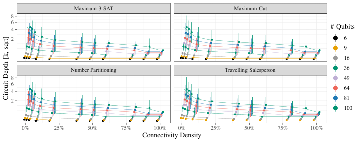
Figure 1: Span of achievable circuit depths for the subject problems in different sizes, plotted over varying degrees of connectivity. Data points for each density are slightly displaced horizontally to make point ranges visible; connecting lines do not provide a fit to the data, but are only used to guide the eye.

IV Experiments

IV-A Setup

In this work, the quantum circuits are designed and transpiled using Qiskit [27]. We study the QAOA-circuits for several instances of the four problems described above after being transpiled to hardware backends with different properties. As a starting point, a backend with 127 qubits is chosen that matches the geometric layout and connectivity of the current IBM-Q devices, the so-called heavy-hex-geometry [28]. The native gate set corresponds to that of IBM-Q, containing the following gates: Rotation $RZ$, phase shift $SX$, Pauli (Not) $X$, and controlled X ($\text{C\raisebox{0.80002pt}{--}}\!X$). In principle, also the influence of noise on the transpilation process could be modelled in Qiskit, which is, however, not in the scope of this work.

We investigate the depth and number of Swap gates of the transpiled circuits depending on the connectivity and size of the backend. The circuit depth measures the overall length of the circuit, taking into account also parallel execution of gates. The Swap gate counts are derived by mapping each circuit a second time using an extended native gate set including the Swap gate. This prevents the latter from being decomposed into other gates.

The connectivity of the backend is measured in terms of a connectivity density

$$c=\frac{N_{C}}{N_{C,\mathrm{max}}},$$ (5)

with $N_{C}$ denoting the total number of edges in the hardware graph and $N_{C,\mathrm{max}}=N(N-1)/2$ the maximal number of edges for $N$ qubits. While $c=1$ describes a device with all-to-all connectivity such as in ideal simulations, the heavy-hex-geometry has a connectivity density of $c\approx 1.8\%$. This value corresponds to each qubit having on average $2.27$ nearest neighbours. In the experiments presented below, the connectivity density is increased by randomly adding connections between pairs of qubits until the desired value is reached. The average number of nearest neighbours per qubit grows linearly with the connectivity density.

IV-B Problem Mapping

All problems in NP can be reduced to Quadratic Unconstrained Binary Optimisation (QUBO) problems. The QUBO formulations in this work follows the Ising formulations given by Lucas [29].

IV-B1 Maximum Cut

MaxCut can be cast using binary variables $x_{i}$, where $x_{i}=1$ indicates that node $i$ belongs to the first subset, and $x_{i}=0$ indicates that it belongs to the second subset. If an edge connecting nodes $i$ and $j$ is part of the cut, then one of $x_{i}$ and $x_{j}$ is equal to zero and the other one is equal to one, resulting in $H_{ij}=(x_{i}+x_{j}-2x_{i}x_{j})$ being $1$, whereas $H_{ij}$ equals $0$ if $x_{i}=x_{j}$. The goal is to find the MaxCut by maximising the sum of $H_{ij}$ over all edges of the graph or in other words minimising the sum over $-H_{ij}$. The optimal solution is the ground state of the Hamiltonian

$$H_{P}=\sum_{(i,j)\in E}(2x_{i}x_{j}-x_{i}-x_{j})$$ (6)

which serves as the objective function for the QAOA algorithm to find the minimum solution.

Setup: The MaxCut problem graphs $G=(V,E)$ were characterised by their number of nodes $N=|V|$, and the graph density $d$, defined as the ratio of the number of edges $|E|$ to the maximum possible number of edges $|E_{\mathrm{max}}|$ in a clique comprising $|V|$ nodes. The value of $d$ ranges from $0$ to $1$ and is set to $d=0.7$ for the experiments in this work. Each node in the graph is represented by one qubit, so the problem size given in numbers of qubits directly corresponds to the number of nodes.

IV-B2 Number Partitioning

NumPart can be reformulated as a QUBO problem using binary variables $x_{i}$ where $x_{i}=1$ indicates that $a_{i}$ belongs to subset S and if $x_{i}=0$, $a_{i}$ belongs to subset T. The objective is given by the Hamiltonian

$$H_{P}=\Big{(}\sum_{i=1}^{n}a_{i}x_{i}\Big{)}^{2}-\Big{(}\sum_{i=1}^{n}a_{i}\Big{)}^{2}$$ (7)

which represents the difference between the sums of S and T. The goal is to find the minimum value of the Hamiltonian, which corresponds to the optimal partitioning of the set.

Setup: The NumPart problem was generated as a list of length $n\in\mathbb{N}$. Each number was generated randomly, and the corresponding field index is represented by one qubit.

IV-B3 Travelling Salesperson

The objective function of the TSP, describing the total length of the tour, is given by the following Hamiltonian:

$$H_{C}=\sum_{i,j\in E,i\neq j}^{N}c_{ij}\sum_{k=1}^{N}x_{i,k}x_{j,k+1}$$ (8)

where $c_{i,j}$ is the distance between nodes $i$ and $j$; $x_{i,k}$ is a binary variable that is equal to $1$ if node $i$ is visited at position $k$ in the tour (and 0 otherwise); and $N$ denotes the total number of nodes in the TSP instance. The sum over $k$ enforces the ordering of the nodes in the tour. Note that $x_{i,N+1}$ is equivalent to $x_{i,1}$, so the tour loops back to the starting node and in our case $c_{i,j}=c_{j,i}$. To ensure that each city is visited exactly once in the tour and that at each position in the tour there is exactly one city, the corresponding penalty terms are added to comprise the final Hamiltonian:

$$H=A\sum_{j=1}^{n}(1-\sum_{k=1}^{N}x_{j,k})^{2}+A\sum_{k=1}^{n}(1-\sum_{j=1}^{N}x_{j,k})^{2})+H_{C},$$ (9)

where $A$ controls the strength of the penalty.

Setup: The TSP problem graphs were represented as a complete, undirected graph (so $c_{i,j}=c_{j,i}$), where the nodes represent the cities and the edges represent the distances between them. A randomly generated distance matrix determines the distances between the cities. For $N$ nodes, we have $N^{2}$ qubits and a $N\times N$ distance matrix. The graph density for TSP is defined analogously to MaxCut and also set to $d=0.7$.

IV-B4 Maximum 3-Satisfiability

To formulate this problem as a QUBO, we introduced three binary variables $y_{i}$, $y_{j}$ and $y_{k}$, where each variable can take the value $0$ or $1$. The Hamiltonian for this problem is given by

$$H=\sum_{i=1}^{m}(1-\frac{1}{2}(y_{i}+y_{j}+y_{k}-1)$$ (10)

where m is the number of clauses. The Hamiltonian is minimised when the number of satisfied clauses is maximised.

Setup: The values for each variable were generated randomly. The number of clauses added to the number of variables equals the number of qubits necessary to represent our QUBO formulation. In our experiments we use a fixed number of $3$ variables per clause. According to Figure 6, the ratio between the number of clauses and number of variables has little to no effect on the circuit depth, suggesting it can be disregarded in the experiments.

IV-C Circuit Mapping

The hardware backend is described by a connectivity graph given in the form of tuples and a native gate set. The transpilation process in Qiskit consists of several steps: First, the circuit is optimised, for instance by combining several single-qubit gates into a single one. Then, all gates which do not belong to the native gate set, such as gates with more than 2 qubits, are decomposed into the native gate set. The next step is to find an optimal placement of the logical qubits in the circuit to the physical qubits of the hardware, which corresponds to a direct mapping of the problem (or algorithm) graph to the hardware graph. Thereby, Swap gates are inserted, if necessary, and the mapping is determined to minimise the number of Swap gates. For the circuits presented here, the standard mapping method of Qiskit has been used, which includes a stochastic placement of Swap gates. After the mapping, the inserted Swap gates are being translated into the native gate set (if necessary), and the circuit is optimised once more, accounting e.g., for possible concatenations of gates.

The aggressiveness of depth optimisation varies between four levels [19] (level $n$ includes all measures of levels $k<n$):

• $0$ (off): Map without optimisation.

• $1$ (light): Collapse adjacent gates that cancel each other.

• $2$ (medium): Noise-adaptive layout, gate cancellation based on gate commutation relationships.

• $3$ (heavy): Replace blocks of gates with (different, yet semantically equivalent) optimised gate sequences.

Our numerical experiments were performed at optimisation level 2, which provides a good trade-off between result optimality and required computational effort. This choice is further justified in Section VI.

V Evaluation

We commence to discuss the outcomes of our numerical experiments in the following, and then find common patterns in the data using statistical analysis techniques.

V-A Numerical Results

V-A1 Circuit Depth and Swap gate Count

The depth of quantum circuits is analogue to classical runtime—the more gates are involved in a circuit, the longer a quantum computation takes—, but also key to understanding the capabilities of NISQ machines, as increasingly deep circuits are subject to growing amounts of noise and decoherence, eventually leading to entirely stochastic results that do not provide information about the problem at hand. Recall that quantum circuits generated for specific problem formulations are produced by a uniform generation mechanism, but vary with instance size and characteristics of the individual instances.

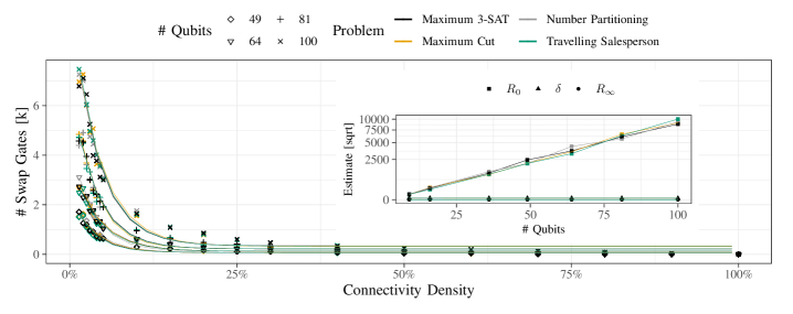
Figure 2: Outer: Empirical observation of Swap gate count decrease with increasing connectivity density (points), together with fits obtained by the negative exponential model (solid lines) for the subject problems. Inset: Corresponding model coefficients.

As one of our goals is to understand the effects of varying degrees of connectivity in (hypothetical) QPUs, first consider Fig. 1, which shows the achievable circuit depths for a given degree of (extended) connectivity for the subject problems in various instance sizes given by the amount of required qubits. Since mapping between logical and physical circuits is performed by a stochastic algorithm, we obtain a range of depths for varying connectivity densities and qubit count. Data points in Figure 1 represent mean values over 20 compilation runs. It is immediately apparent that even small increases in circuit depth over the base connectivity of IBMQ’s heavy hex topology lead to considerable reduction of the circuit depth in a similar way for all of the problem types considered here. Likewise result variability increases considerably towards smaller degrees of connectivity. Both, strength of variability and circuit depth, converge for densities exceeding 25%.

Figure 2 shows the amount of Swap gates that are required for a given connectivity density (we address the inset in Sec. V-B below). Since Swap gates are necessary to bring qubits into physical adjacency when multi-qubits operations must be applied on topologically not adjacent qubits, they can be seen as overhead that arises from restricted connectivity densities. As the figure shows, zero Swap gates are required when the density reaches 1.0, as the need to logically move qubits by swapping them around in the circuit does not arise in this case. Similar to circuit depth, we can observe a steep decline in Swap gate count with increasing connectivity density, and a plateauing of the count form densities of about $30\%$ onwards.

V-B Statistical Modelling

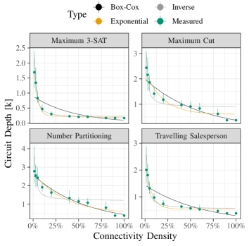
Figure 3: Comparing models (inverse, Box-Cox, negative exponential; solid lines) against the empirically measured data (points). The graph shows problem instances each requiring 64 qubits; graphs for other sizes exhibit similar characteristics and are available on the supplementary website.

While it is obvious from Figures 1 and 2 that even slightly improved connectivity density results in substantial reductions on circuit depth independent of the specific problem, it is pertinent to further characterise this empirical observation. To find simple models that accurately describe the observed phenomena, we fit statistical models to the available data.

The sharp decrease of circuit depth with increasing connectivity density, modelled in general by a functional dependency of the form $d(\varrho)=f_{\text{P}}(\varrho)$ (where P denotes specialisation for a specific problem) suggests an inverse ($f(\varrho)\sim 1/\varrho$) or negative exponential ($f(\varrho)\sim\exp(-\varrho)$) relationship. The empirical results for these ansätze (linear univariate regression [30] for the inverse relationship, non-linear regression [31] for the negative exponential), together with a linear regression fit based on a Box-Cox transformation [32] of the data, is shown in Fig. 3. Visually, it is obvious that the linear regression based approaches result in a sub-optimal match between model and data, whereas the negative exponential ansatz

$$d(\varrho)=R_{\infty}+(R_{0}-R_{\infty})\cdot e^{-\exp(\delta)\cdot\varrho}$$ (11)

describes the data very well. Based on the data for each subject problem, parameters $R_{0}$, $R_{\infty}$ and $\delta$ are obtained for varying connectivity densities. $R_{\infty}$ denotes the horizontal asymptote towards large values of the connectivity density, $R_{0}$ is the (extrapolated) circuit depth estimate for vanishing connectivity density at $\varrho=0$, offset by $R_{\infty}$. Coefficient $\delta$ represents the natural logarithm of the exponential rate constant, and characterises the speed of decline with increasing connectivity density.

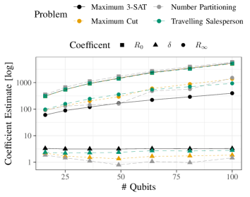
Figure 4: Coefficients for the non-linear negative exponential fit described by Eq. 11 to the circuit depths for all subject problems over varying instance sizes. Connecting lines have no significance, and are only used to guide the eye.

Consider Figure 4, which summarises the evolution of model parameters for the circuit depth with increasing instance sizes for all subject problems. Note that for each problem and instance size, we numerically compute circuit depths for a range of connectivity densities, and then fit Eq. 11 to the data. Consequently, each combination of problem and instance size delivers three parameters. The evolution of these parameters with increasing instance sizes is shown in the figure.

Apart from some smaller variations for NumPart, the rate constant $\delta$ is stable across instance sizes—that means that exponential improvements in circuit depth with increasing connectivity density are achieved nearly uniformly across the full spectrum of instance sizes. As gains are mostly independent of the problem, we hypothesise that this behaviour holds as a general law for QAOA-based approaches. Circuit depths in the limits of zero and full connectivity, obviously increase with increasing problem size. It is however important to observe that the evolution is also very similar across subject problems, again hinting at a general property of QAOA circuits.

The inset in Fig. 2 can be interpreted similarly, except that we use Swap gate counts instead of circuit density as dependent quantity for the model in Eq. 11. Since it is an a-priori invariant that the Swap gate count needs to reach zero for full connectivity (qubits do not need to be swapped around if interactions between any possible pair can be implemented natively), we fit a restricted form of Eq. 11 where the asymptote $R_{\infty}$ is constrained to vanish. The obtained parameters show even better agreement across subject problems than for the circuit depth, which can be explained by the fact that Swap gates constitute “overhead” gates to compensate for connectivity deficiencies. As our results show, this impacts all problems equally. Yet, the observed exponential decrease with increasing connectivity density underlines that even small changes have substantial impact on QC utility.

V-C Implications for Co-Design

In the previous section we have seen that the circuit depth as well as the number of inserted Swap gates is already reduced by a significant amount when increasing the connectivity density to intermediate values of about $30\%$. This value increases slightly with the problem size, but does not depend on the problem type, as shown in Fig. 4. Overall, we can state that full connectivity is not essential to decrease the resource requirements for the considered QAOA circuits.

In general, a quantum computing device with connectivity density between $10\%$ to $50\%$ would be an appropriate choice for all of the four problem types. The Swap gate overhead might be reduced further, if also the geometric layout of the hardware graph directly matches that of the problem graph, opposed to randomly adding connections as done in this work. A connectivity density of $c=10\%$ corresponds to each qubit being connected to $15$ nearest neighbours on average, for $c=50\%$ this increases to $64$ neighbours. Apart from the reduced number of gates in the circuit, a higher qubit connectivity is desirable for implementing efficient error-correction schemes which in turn require a lower overhead in the number of physical qubits needed to encode a logical qubit, such as low-density parity check (LDPC) codes [33, 22].

The connectivity of currently available quantum computers depends on the type of quantum hardware being used. Architectures based on superconducting qubits, such as the devices built by IBM and Google, are currently limited to nearest neighbour connectivity (so $c\approx 3.2\%$) [34, 15, 35]. There exist several ideas to increase the connectivity. One common approach is to couple several qubits to a quantum bus, either directly via tuning their frequencies in and out of resonance with the bus [36], or indirectly via additional flux qubits [34], which are variably tuned. The latter architecture has the advantage of lower cross-talk and longer coherence times, since the data qubits can be operated at their optimal frequencies. Other ideas include using sparse connections but with non-trivial topologies, extending the architecture to 3D or using long cables to connect distant qubits [22]. With the quantum bus setup proposed in [34], the connectivity could theoretically be increased such that two-qubit-gates can be performed between all pairs of qubits, superseding the insertion of Swap gates at all. Nevertheless, realising such a setup with only an intermediate connectivity, as suggested by our findings, will in any case benefit the practical implementation.

In general, increasing the number of connections between qubits can lead to a higher probability for crosstalk. This term describes unwanted interaction between qubits or between qubits and the control signals, which means that a gate pulse can effect other than the target qubit(s) or local gate operations are disturbed by other gate operations applied in parallel. These effects are especially detrimetal for implementing error correction, which assumes that gate errors only affect the state of the target qubits. For superconducting qubits, crosstalk can be reduced by using qubits with tunable frequencies (see [34]) and / or tunable couplers to switch connections dynamically on and off. In addition, optimizing the pattern of tunable qubit frequencies and gate schedules via software can also lead to substantial improvements [37]. On the other hand, architectures with fixed-frequency qubits and fixed couplers like IBM-Q that do not allow for such optimisation suffer from fewer sources of noise. In this case, optimised gate schedules are being used to minimise crosstalk [38].

Quantum computers based on cold neutral atoms and Rydberg-interactions already feature a higher connectivity of about $1$:$10$ to $1$:$20$ in 2D- and 3D-layouts [21], which would correspond to $c\approx 8$-$16\%$ for the heavy-hex-based layout. The connectivity can be further increased by using higher energy levels for the Rydberg interaction, which, however, might lead to a higher susceptibility to noise and become technically challenging. Another approach is shuttling of atoms during the computation to allow for two-qubit-gates between arbitrary pairs of qubits [39]. In general, crosstalk is quite low for neutral atom qubits [40, 41], since their distances can be made large enough to avoid unwanted excitations of spectator qubits. Also, increasing the qubit connectivity is not necessarily related to higher crosstalk for this platform.

In contrast to the two previous examples, trapped ion quantum computers are characterized by an all-to-all connectivity, which means that two-qubit gates can be performed between each pair of qubits, but also up to $20$ qubits can be entangled [42]. On the other hand, ion trap setups are more difficult to scale to larger numbers of qubits. The most common technique stores ions in a linear string and is limited to qubits numbers in the range of $50$. This has to be compared to superconducting qubits and neutral atoms, which currently offer up to $\approx 400$ [43] and $\approx 100$ [21, 39] qubits, respectively, and, in the latter case, are also easier to scale. Ion strings with larger number of ions are expected to suffer from lower gate speeds, higher crosstalk and background noise [44]. To realise trapped-ion devices with larger number of qubits, mainly two different approaches exist: coupling several linear traps via photonic interconnects or shuttling of ions in a 2D trap. While the first approach is more simple to realise, it is affected by higher crosstalk due to residual illumination of ions which are not targeted by a gate operation. Crosstalk can be reduced by careful design of pulse sequences or improved laser focusing, as well as by using refocusing schemes [45]. While the first option can be broadly attributed to the software domain, the latter two options are deeply intertwined with the core physical realisation of QPUs.

Finally, to find the most suitable platform for a quantum program, a trade-off between several properties such as the connectivity, number of qubits or error-rates has to be made.

VI Threats to Validity

VI-A External Validity

Our scope is limited to the Qiskit compiler and the base topology of IBM-Q devices. It is important to note that using different compilers may result in varying circuit properties (see Salm et al. [46]), which means that our findings may not be applicable to other compilers. Additionally, different topologies may yield different outcomes. Furthermore, we only consider QAOA. There are other (variational) quantum algorithms as well as different types of the QAOA algorithms, that tackle NP optimisation problems [47]. While it is possible to model the impact of noise on the transpilation process in Qiskit, which would effect the circuit depth, it falls outside the scope of this work [48].

VI-B Internal Validity

Our observations rely on controlled numerical experiments that depend on explicit parameters, but may also be influenced by confounding factors. In the following, we consider various possible confounding factors, and find that they pose moderate to no risk to the validity of our study.

VI-B1 Influence of Mapping Optimisation

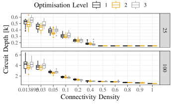
Figure 5: Distribution of circuit depth for two instance sizes (25 and 100 qubits) over connectivity density for varying optimisation levels obtained with the Qiskit compiler 0.41.1, see the replication package on the supplementary website for details) for the travelling salesperson problem.

Since the circuit mapping (transpilation) problem is known to be NP-complete by itself (see, e.g., [48]), it is unavoidable to use approximation techniques that cannot guarantee optimal results in feasible time, and therefore require precise characterisation. In particular, there is the risk that the technical choice of optimisation level could impact our general conclusions; likewise, different compiler/mapping approaches could influence behaviour.

Consider Figure 5, which compares mapping results with different optimisation levels for medium and large problem instances requiring 25 and 100 qubits for the TSP (identical observations can be made for the other subject problems). All levels follow the exponential decrease pattern, with relatively small improvements of optimisation level 3, although it is also clear that the highest optimisation level does not guarantee smallest circuits, neither averaged nor overall. As the highest optimisation level implies considerably increased simulation times (days instead of hours), we find our choice of optimisation level 2 justified. While there are many other approaches to circuit compilation that we cannot compare in detail in the scope of this work, the results of Salm et al. [46], together with results that take differences for mapping practical problems between the most widespread compilers into account [49], indicate that the risk of observing a qualitatively different scaling behaviour is absolute minor, though.

VI-B2 Influence of Instance Properties

Quantum circuits for a given problem are constructed using a uniform mechanism that depends on problem size, but also on the properties of the instance itself. As the observed exponential decrease in circuit depth might depend on the latter properties, we explore a varying set of parameters for problem MAX-3SAT. Boolean satisfiability is known to exhibit marked differences in computational complexity depending on the ratio $\alpha=|C|/|V|$ between the number of variables $|V|$ and clauses $|C|$ (see, e.g., Refs [50]). Fig. 6 shows how the circuit depth decreases with increasing connectivity density for random instances of the problem that are constrained to a given value of $\alpha$. We scan across values of $\alpha$ that represent regions where instances are either trivially to solve by guessing ($\alpha\in[0,3.5]$) or finding contradictory assignments that show non-solubility ($\alpha\in[4.9,11]$), as well as the region around $\alpha\approx 4.2$ that is known to contain computationally hard problem instances.

The inset shows that all three model coefficients $R_{0},R_{\infty}$ and $\delta$ as given in Eq. 11 are are in good agreement with a constant value for each across the whole spectrum of $\alpha$, indicating no influence of the specific instance. Consequently, we deem this risk minor to negligible. For this particular assessment, it was not necessary to test other problem sizes, as $\alpha$ determines the complexity of the Max3Sat problem.

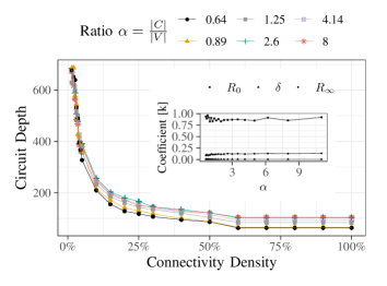
Figure 6: Empirically observed circuit depth degradation for MAX-3SAT on 36 variables, with varying degrees of $\alpha$ (outer plot; see the main text for an explanation of this parameter), and the coefficients obtained for Eq. 11 (inset). The outer plot shows mean circuit depths obtained with 20 samples per data point and omit ranges to reduce visualisation clutter, while the model fit is obtained from the full data set. Connecting lines are used to guide the eye.

VI-B3 Influence of Backend Size

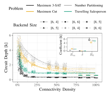
Figure 7: Empirical observations for circuit depth for problems with constant size of 36 qubits with varying backend sizes (geometrically extrapolated from the IBM-Q heavy-hex backend), together with nonlinear regression fits of the model in Eq. 11 (we augment the empirical observations with a slight horizontal jitter to reduce overplotting. Inset: Distribution of regression coefficients.

Our numerical experiments are performed using a constant backend size of $127$ qubits, so the ratio of the problem size to the backend size varies. If the problem is much smaller than the backend, several mappings of logical to physical qubits are possible. We empirically study whether this influences the circuit depth by uniformly scaling the backend size, while retaining the connectivity structure of the heavy-hex geometry, which is composed of a certain number of rows and columns containing interconnected rings. Figure 7 shows circuit depths for varying backend sizes, whose geometry has been consistently extended from the IBM-Q Washington architecture with 127 qubits. Backend sizes are specified in the form $[n,m]$, where $n$ denotes the number of rows, and $m$ the number of columns (details in the replication package on the supplementary website). This creates backends ranging from 143 ($6\times 4$) to 297 ($8\times 6$) qubits.

For none of the problems, the exponential decrease for increasing connectivity density changes; there is practically no influence of the increased backend size for Max 3-SAT and TSP. For MaxCut and NumPart, the asymptotes vary moderately depending on backend size, yet the differences are only relevant for connectivity densities exceeding $50\%$. However, since the models overestimate the connectivity densities compared to empirical observations, we err—if at all—on the side of caution. These observations are also backed by the regression model coefficients, whose distribution for each subject problem is shown in the inset. Especially the rate parameter is extremely narrowly distributed, which means that the exponential decrease with increasing connectivity density is independent of the base backend size. Consequently, we deem this threat minor.

VII Discussion & Outlook

In conclusion, our results show that an all-to-all connectivity is not necessary to achieve near-optimal circuit depth for all subject problems. Even small changes to the density can lead to significant improvements, particularly across different problem sizes and types. Lower connectivity between qubits, lower circuit depth and lower gate counts can help scale quantum systems, as the number of interactions between qubits, the number of quantum gates required to execute algorithms and the overall complexity of the system is decreased. Therefore it becomes easier to maintain coherence and reduce the probability of errors and decoherence, which are crucial factors in building scalable quantum computing systems [51]. We have identified an underlying effective model, which exhibits an exponential decrease in circuit depth with increasing connectivity uniformly across all instance sizes. This suggest that our findings may be applicable to other problem domains. Our results also point towards the construction of better problem-adapted QPUs as a possible step towards practical applications of quantum computing. The fact that all problems demonstrate a consistent exponential decrease in circuit depth as connectivity density rises is a highly encouraging and promising observation. This trend is true for all investigated problems. Further research is required to explore the full potential of our findings and understand the optimal topologies as well as the effects on scalability for specific problems and problem classes. This includes a comprehensive analysis of the effects of noise and different topology layouts. Moreover, it is important to incorporate more refined physical models that better capture the physical trade-offs involved. Finally, it is important to emphasise the importance of hardware-software co-design for achieving scalability in quantum computing. As we continue to explore new algorithms and applications, it will be necessary to develop hardware and software in tandem to ensure that they are optimised for each other.

Acknowledgements This work is supported by the German Federal Ministry of Education and Research within the funding program Quantentechnologien – von den Grundlagen zum Markt, contract number 13N16092.

References

- [1] I. Sax, S. Feld et al., “Approximate approximation on a quantum annealer,” in Proceedings of the 17th ACM International Conference on Computing Frontiers, ser. CF ’20. New York, NY, USA: Association for Computing Machinery, 2020, p. 108–117. [Online]. Available: https://doi.org/10.1145/3387902.3392635
- [2] A. Bayerstadler, G. Becquin et al., “Industry quantum computing applications,” EPJ Quantum Technology, vol. 8, no. 1, 11 2021. [Online]. Available: https://epjquantumtechnology.springeropen.com/track/pdf/10.1140/epjqt/s40507-021-00114-x.pdf
- [3] V. T. Paschos, “An overview on polynomial approximation of NP-hard problems,” The Yugoslav Journal of Operations Research, vol. 19, no. 37, pp. 3–40, 2009. [Online]. Available: http://eudml.org/doc/261608
- [4] D. S. Hochbaum, Ed., Approximation Algorithms for NP-Hard Problems. USA: PWS Publishing Co., 1996.
- [5] E. Farhi, J. Goldstone, and S. Gutmann, “A quantum approximate optimization algorithm,” 2014. [Online]. Available: https://arxiv.org/abs/1411.4028
- [6] J. S. Clarke, “An optimist’s view of the 4 challenges to quantum computing,” Quantum, p. 2, Mar 2019. [Online]. Available: https://spectrum.ieee.org/an-optimists-view-of-the-4-challenges-to-quantum-computing
- [7] K. Wintersperger, H. Safi, and W. Mauerer, “QPU-System Co-Design for Quantum HPC Accelerators,” in Proceedings of the 35th GI/ITG International Conference on the Architecture of Computing Systems. Gesellschaft für Informatik, 8 2022.
- [8] G. Li, A. Wu et al., “On the co-design of quantum software and hardware,” in Proceedings of the Eight Annual ACM International Conference on Nanoscale Computing and Communication, ser. NANOCOM ’21. New York, NY, USA: Association for Computing Machinery, 2021. [Online]. Available: https://doi.org/10.1145/3477206.3477464
- [9] W. Mauerer and S. Scherzinger, “1-2-3 reproducibility for quantum software experiments,” Q-SANER@IEEE International Conference on Software Analysis, Evolution and Reengineering, 2022.
- [10] K. Temme, S. Bravyi, and J. M. Gambetta, “Error mitigation for short-depth quantum circuits,” Physical Review Letters, vol. 119, no. 18, nov 2017. [Online]. Available: https://doi.org/10.1103%2Fphysrevlett.119.180509
- [11] V. Akshay, D. Rabinovich et al., “Parameter concentrations in quantum approximate optimization,” Physical Review A, vol. 104, no. 1, jul 2021. [Online]. Available: https://doi.org/10.1103%2Fphysreva.104.l010401
- [12] P. C. Lotshaw, T. Thien Nguyen et al., “Scaling quantum approximate optimization on near-term hardware,” Scientific Reports, vol. 12, no. 1, july 2022. [Online]. Available: https://doi.org/10.1038%2Fs41598-022-14767-w
- [13] R. Wille and L. Burgholzer, “MQT QMAP: efficient quantum circuit mapping,” CoRR, vol. abs/2301.11935, 2023. [Online]. Available: https://doi.org/10.48550/arXiv.2301.11935
- [14] A. Kandala, A. Mezzacapo et al., “Hardware-efficient variational quantum eigensolver for small molecules and quantum magnets,” Nature, vol. 549, no. 7671, pp. 242–246, sep 2017. [Online]. Available: https://doi.org/10.1038%2Fnature23879
- [15] N. M. Linke, D. Maslov et al., “Experimental comparison of two quantum computing architectures,” Proceedings of the National Academy of Sciences, vol. 114, no. 13, pp. 3305–3310, mar 2017. [Online]. Available: https://doi.org/10.1073%2Fpnas.1618020114
- [16] R. Shaydulin and Y. Alexeev, “Evaluating quantum approximate optimization algorithm: A case study,” in 2019 Tenth International Green and Sustainable Computing Conference (IGSC). IEEE, oct 2019. [Online]. Available: https://doi.org/10.1109%2Figsc48788.2019.8957201
- [17] S. Feld, C. Roch et al., “A hybrid solution method for the capacitated vehicle routing problem using a quantum annealer,” M. S. Sarandy, Ed., vol. 6. Frontiers Media SA, 6 2019. [Online]. Available: https://arxiv.org/abs/1811.07403
- [18] D. Venturelli, M. Do et al., “Quantum circuit compilation: An emerging application for automated reasoning,” in Proceedings of the Scheduling and Planning Applications Workshop (SPARK2019), 2019.
- [19] Qiskit Transpiler Documentation. https://qiskit.org/documentation/apidoc/transpiler.html.
- [20] C. D. Bruzewicz, J. Chiaverini et al., “Trapped-ion quantum computing: Progress and challenges,” Applied Physics Reviews, vol. 6, no. 2, p. 021314, 2019. [Online]. Available: https://doi.org/10.1063/1.5088164
- [21] L. Henriet, L. Beguin et al., “Quantum computing with neutral atoms,” Quantum, vol. 4, p. 327, Sep. 2020.
- [22] S. Bravyi, O. Dial et al., “The Future of Quantum Computing with Superconducting Qubits,” Journal of Applied Physics, vol. 132, no. 16, p. 160902, Oct. 2022. [Online]. Available: https://aip.scitation.org/doi/abs/10.1063/5.0082975
- [23] S. Slussarenko and G. J. Pryde, “Photonic quantum information processing: A concise review,” Applied Physics Reviews, vol. 6, no. 4, p. 041303, 2019. [Online]. Available: https://doi.org/10.1063/1.5115814
- [24] D. P. Williamson and D. B. Shmoys, The Design of Approximation Algorithms. Cambridge University Press, 2011.
- [25] A. Alridha, A. M. Salman, and A. Sabah Al-Jilawi, “The applications of np-hardness optimizations problem,” Journal of Physics: Conference Series, vol. 1818, no. 1, p. 012179, mar 2021. [Online]. Available: https://dx.doi.org/10.1088/1742-6596/1818/1/012179
- [26] C. Pierluigi and K. Viggo, “A compendium of np optimization problems,” 1994, 2005. [Online]. Available: https://www.csc.kth.se/tcs/compendium/
- [27] Abby-Mitchell, H. Abraham et al., “Qiskit: An open-source framework for quantum computing,” 2021.
- [28] The IBM Quantum heavy hex lattice. https://research.ibm.com/blog/heavy-hex-lattice.
- [29] A. Lucas, “Ising formulations of many np problems,” Frontiers of Physics in China, vol. 2, pp. 5–, 2014.
- [30] L. Fahrmeir, T. Kneib et al., Regression: Models, Methods and Applications. Berlin: Springer-Verlag, 2013.
- [31] D. Bates and D. Watts, Nonlinear regression analysis and its applications, ser. Wiley series in probability and mathematical statistics. New York: Wiley, 1988. [Online]. Available: http://gso.gbv.de/DB=2.1/CMD?ACT=SRCHA&SRT=YOP&IKT=1016&TRM=ppn+025625357&sourceid=fbw_bibsonomy
- [32] W. N. Venables and B. D. Ripley, Modern Applied Statistics with S, 4th ed. New York: Springer, 2002, iSBN 0-387-95457-0. [Online]. Available: https://www.stats.ox.ac.uk/pub/MASS4/
- [33] N. P. Breuckmann and J. N. Eberhardt, “Quantum Low-Density Parity-Check Codes,” PRX Quantum, vol. 2, no. 4, p. 040101, Oct. 2021. [Online]. Available: https://link.aps.org/doi/10.1103/PRXQuantum.2.040101
- [34] R. Stassi, M. Cirio, and F. Nori, “Scalable quantum computer with superconducting circuits in the ultrastrong coupling regime,” npj Quantum Information, vol. 6, no. 1, p. 67, Aug. 2020. [Online]. Available: https://www.nature.com/articles/s41534-020-00294-x
- [35] R. Acharya, I. Aleiner et al., “Suppressing quantum errors by scaling a surface code logical qubit,” Nature, vol. 614, no. 7949, pp. 676–681, Feb. 2023. [Online]. Available: https://doi.org/10.1038/s41586-022-05434-1
- [36] C. Song, K. Xu et al., “Generation of multicomponent atomic schrödinger cat states of up to 20 qubits,” Science, vol. 365, no. 6453, pp. 574–577, 2019. [Online]. Available: https://www.science.org/doi/abs/10.1126/science.aay0600
- [37] Y. Ding, P. Gokhale et al., “Systematic Crosstalk Mitigation for Superconducting Qubits via Frequency-Aware Compilation,” in 2020 53rd Annual IEEE/ACM International Symposium on Microarchitecture (MICRO). Athens, Greece: IEEE, Oct. 2020, pp. 201–214. [Online]. Available: https://ieeexplore.ieee.org/document/9251858/
- [38] P. Murali, D. C. Mckay et al., “Software mitigation of crosstalk on noisy intermediate-scale quantum computers,” in Proceedings of the Twenty-Fifth International Conference on Architectural Support for Programming Languages and Operating Systems, ser. ASPLOS ’20. New York, NY, USA: Association for Computing Machinery, 2020, p. 1001–1016. [Online]. Available: https://doi.org/10.1145/3373376.3378477
- [39] D. Bluvstein, H. Levine et al., “A quantum processor based on coherent transport of entangled atom arrays,” Nature, vol. 604, no. 7906, pp. 451–456, Apr. 2022. [Online]. Available: https://www.nature.com/articles/s41586-022-04592-6
- [40] T. Xia, M. Lichtman et al., “Randomized benchmarking of single-qubit gates in a 2d array of neutral-atom qubits,” Phys. Rev. Lett., vol. 114, p. 100503, Mar 2015. [Online]. Available: https://link.aps.org/doi/10.1103/PhysRevLett.114.100503
- [41] T. M. Graham, M. Kwon et al., “Rydberg-mediated entanglement in a two-dimensional neutral atom qubit array,” Phys. Rev. Lett., vol. 123, p. 230501, Dec 2019. [Online]. Available: https://link.aps.org/doi/10.1103/PhysRevLett.123.230501
- [42] N. Friis, O. Marty et al., “Observation of entangled states of a fully controlled 20-qubit system,” Phys. Rev. X, vol. 8, p. 021012, Apr 2018. [Online]. Available: https://link.aps.org/doi/10.1103/PhysRevX.8.021012
- [43] IBM Quantum computer with 433 qubits. https://newsroom.ibm.com/2022-11-09-IBM-Unveils-400-Qubit-Plus-Quantum-Processor-and-Next-Generation-IBM-Quantum-System-Two.
- [44] K. R. Brown, J. Kim, and C. Monroe, “Co-designing a scalable quantum computer with trapped atomic ions,” npj Quantum Information, vol. 2, no. 1, p. 16034, Nov. 2016. [Online]. Available: https://doi.org/10.1038/npjqi.2016.34
- [45] P. Parrado-Rodríguez, C. Ryan-Anderson et al., “Crosstalk Suppression for Fault-tolerant Quantum Error Correction with Trapped Ions,” Quantum, vol. 5, p. 487, Jun. 2021. [Online]. Available: https://doi.org/10.22331/q-2021-06-29-487
- [46] M. Salm, J. Barzen et al., “Automating the comparison of quantum compilers for quantum circuits,” in Service-Oriented Computing, J. Barzen, Ed. Cham: Springer International Publishing, 2021, pp. 64–80.
- [47] M. Cerezo, A. Arrasmith et al., “Variational quantum algorithms,” Nature Reviews Physics, vol. 3, no. 9, pp. 625–644, aug 2021. [Online]. Available: https://doi.org/10.1038%2Fs42254-021-00348-9
- [48] A. Paler, A. Zulehner, and R. Wille, “Nisq circuit compilation is the travelling salesman problem on a torus,” Quantum Science and Technology, vol. 6, no. 2, p. 025016, mar 2021. [Online]. Available: https://dx.doi.org/10.1088/2058-9565/abe665
- [49] M. Schönberger, S. Scherzinger, and W. Mauerer, “Ready to leap (by co-design)? join order optimisation on quantum hardware,” in Proceedings of ACM SIGMOD/PODS International Conference on Management of Data, 2023.
- [50] T. Krüger and W. Mauerer, “Quantum annealing-based software components: An experimental case study with SAT solving,” Q-SE@ICSE, 2020. [Online]. Available: https://arxiv.org/abs/2005.05465
- [51] D. Reilly, “Challenges in scaling-up the control interface of a quantum computer,” in Proceedings of 2019 IEEE International Electron Devices Meeting IEDM, 12 2019, pp. 31.7.1–31.7.6.
- [52] R. Wille, L. Burgholzer, and A. Zulehner, “Mapping quantum circuits to ibm qx architectures using the minimal number of swap and h operations,” in Proceedings of the 56th Annual Design Automation Conference 2019, ser. DAC ’19. New York, NY, USA: Association for Computing Machinery, 2019. [Online]. Available: https://doi.org/10.1145/3316781.3317859
- [53] S. Sivarajah, S. Dilkes et al., “t: a retargetable compiler for nisq devices,” Quantum Science and Technology, vol. 6, no. 1, p. 014003, nov 2020. [Online]. Available: https://dx.doi.org/10.1088/2058-9565/ab8e92
- [54] Y. A. Kharkov, A. Ivanova et al., “Arline benchmarks: Automated benchmarking platform for quantum compilers,” ArXiv, vol. abs/2202.14025, 2022.