T-ADAF: Adaptive Data Augmentation Framework for Image Classification Network based on Tensor T-product Operator

Abstract

Image classification is one of the most fundamental tasks in Computer Vision. In practical applications, the datasets are usually not as abundant as those in the laboratory and simulation, which is always called as Data Hungry. How to extract the information of data more completely and effectively is very important. Therefore, an Adaptive Data Augmentation Framework based on the tensor T-product Operator is proposed in this paper, to triple one image data to be trained and gain the result from all these three images together with only less than 0.1% increase in the number of parameters. At the same time, this framework serves the functions of column image embedding and global feature intersection, enabling the model to obtain information in not only spatial but frequency domain, and thus improving the prediction accuracy of the model. Numerical experiments have been designed for several models, and the results demonstrate the effectiveness of this adaptive framework. Numerical experiments show that our data augmentation framework can improve the performance of original neural network model by 2%, which provides competitive results to state-of-the-art methods.

Keywords: Data Augmentation, tensor T-product, Image Classification, Neural Network, Adaptive Framework.

AMS Subject Classifications: 15A18, 65F10, 65F15, 68T45.

1 Introduction

The image classification issue has always been one of the most important problems in the field of the computer vision. Many researchers have focused on achieving improvements in prediction accuracy of image classification. On this long and challenging road, many important branches have been derived out and several worthy research topics have been provided. Since neural networks were firstly proposed in the twentieth century, scientists have inestigated this fundamental problem for plenty of years. However, the early neural network models have not been applied on large-scale applications due to the limitations of computational power and insufficient data sets. The proposal of back-propagation algorithm [1] and the rapid increase of computational power in recent years have made it possible to train neural networks, especially deep neural networks. With more layers of the neural network models designed, the structure is becoming more complex and performance of the model is becoming better.

A lot of researches [2, 3, 4, 5, 6, 7, 8, 9, 10, 11] are devoted to improving the accuracy rate of image classification, such as Convolutional Neural Network (CNN) [12, 13], Vision Transformer [14] and their variants. The LeNet-5 was proposed to solve the problem of handwritten digit classification, which was an early application of Convolutional Neural Networks in the field of image recognition. In recent years, the application of attention mechanisms [15] has further improved the performance of models, in the field of not only Computer Vision [16] but also Natural Language Processing [17]. By stacking attention modules, Vision Transformer contains more model parameters and further improves the ability to acquire and preserve information. However, in practice, the number of parameters and complexity of the model are often limited by factors such as memory, CPU or GPU, etc.

Different from the relatively idealized conditions in the laboratory, algorithm scientists often face a variety of problems such as data hungry, model complexity limitation and constraint by computational power in practical application [18]. First of all, many practical scenarios are unlikely to provide enough data for neural networks to learn, which leads to the problems of data hungry. Secondly, the limited running memory and storage space do not support the stacking of neural network layers and the increasing in the number of parameters. Meanwhile, the data often changes in real time and the models need to output results as soon as possible, so there is no time to manually adjust the hyper-parameters. Last but not least, due to the impact of insufficient computational power, such as GPU resources, it is impossible to have almost infinite iteration time as in the laboratory. The Adaptive Data Augmentation Framework proposed in this paper solves the above problems. On the premise of increasing the number of parameters by less than one thousandth and keeping the hyper-parameters unchanged, this data augmentation framework not only improves the prediction accuracy of image classification but also reduces the number of iterations required to achieve the highest prediction accuracy.

Data hungry is a problem which is often encountered in practical tasks. Many domains, such as science and medicine, would hardly have datasets the size of ImageNet. The size of dataset limits the ability of model to obtain information from the training set, which affects the final performance of the prediction results. In response to the problem of data hungry, many people have proposed data augmentation algorithms. Among them, the direct operations on an image include flip, rotation, scaling, cropping and shifting. In addition, adding Gaussian noise can also achieve the effect of data augmentation. However, these data augmentation techniques prohibit dynamic adjustment of the parameters during the training process. Thus the effect of the whole augmentation technique has been determined at the beginning of iterations. Therefore, adaptive trainable data augmentation algorithms become a necessary research topic [19]. It is worth mentioning that the Generative Adversarial Network (GAN) [20, 21, 22] is a very delicately designed neural network model. GAN enables one network to generate samples that are different from the training set and hard to distinguish from the other network, and uses two subneural networks to compete against each other during the training process to reach a Nash equilibrium. In the process of training, the prediction accuracy is improved, and it can also be regarded as an adaptive data augmentation framework.

In this paper, our idea mainly comes from exploring the complementarity of tensor operators and deep neural networks in the ability of image information extraction. We notice that neural networks built using only tensor operators [23] do not reach the SOTA (State of the Art) level. We think that the reason may lie in the insufficient ability of tensor operators to extract local features. Meanwhile, the traditional deep learning network has a certain space for improvement in the extraction of global image information, such as the relative positions of pixels and the potential correlation between pixels [24]. As an RGB image, a digitized image should be considered as a third-order tensor. It is therefore natural to ask whether it is feasible to treat the image as a three-dimensional whole and add it to the operation of the neural network model. There have been several papers proposing tensor deep learning models or tensor high-dimensional functions and achieving some results before us [25, 26, 27, 23, 28]. However, the complexity of tensor computation and the ability of pure tensor neural networks to capture local features are two important constrains. Fortunately, the T-product operator is introduced to deal with problems related to third-order tensors. Before that, operators could cause a lot of problems with the curse of dimensionality or too much complexity, such as Einstein product and outer product.

We combine T-product and original learning model for better properties and higher accuracy, where the T-product operator obtains the macroscopic features of the whole, and the original model obtains the microscopic features of the detailed parts. Different from the existing Tensor Network or Tensor Neural Network [29, 30, 31, 32], we propose an Adaptive Data Augmentation Framework based on the tensor T-product (T-ADAF). With only increasing the number of parameters by less than 0.1%, the augmentation of the three-dimensional tensor data of the image is achieved by the T-product operator in a structure-preserving manner, giving three times the amount of data for the original model to be enhanced. Since the deep learning model is not completely discarded, the T-product operator and the model are tightly coupled to obtain richer features of image data, not only global but also local features, not only in spatial domain but also in frequency domain. The numerical experiments will demonstrate the effectiveness of our framework.

The innovation and contribution of this paper can be summarized as follows.

• This paper proposes an novel adaptive data augmentation framework to solve the problem of data hunger, extracting more fundamental features.

• This paper explores the application of tensor T-product operator in image classification tasks and obtains the SOTA results. According to the references we collect, few experimental results have been disclosed in the literature.

• The prediction accuracy is improved on the premise that the number of model parameters is rarely increasing. This has great practical and theoretical value for many miniaturized deep learning tasks, with storage or memory limited.

Moreover, the advantages of the adaptive data augmentation framework proposed in this paper can be listed here.

• User Friendliness. All of image classification networks, $\mathcal{F}$, can be considered as a function space, $\mathscr{F}=\{\mathcal{F}\}$, and T-ADAF can be considered as a functional, $\Theta$, on the network function space, $\mathscr{F}$. Any model can be embedded in this framework, with all hyperparameters of the original model unchanged. At the same time, the framework only increases less than one thousandth of the original model parameters. This provides great convenience for the use of the framework.

• Better Performance. The framework adds the T-product tensor operator on the premise of retaining the advantages of the original deep learning network. This framework can provide three times the amount of data for the model, while improving the model’s performances for image data. Meanwhile, T-ADAF is adaptive and the tensor parameters in framework are designed as learnable parameters during training process to be more suitable for classification models.

• More Complete Information Extraction. In this framework, the original model processes signals in the spatial domain and concentrates more on local features, while the T-Product module processes signals in the frequency domain and pays more attention on global features. Scientists can adjust the weights to determine relative importances on T-Product module and original model.

This paper is organized as follows. In Section 2, some fundamental definitions, properties and notations of T-product operator are listed for convenience. Besides, some main results are reviewed. Adaptive Data Augmentation Framework is gained in Section 3. Numerical experiments are designed to compare the model to be promoted with our Adaptive Data Augmentation Framework respectively in Section 4. Finally, in Section 5, we analyze the results and indicate the advantages of Adaptive Data Augmentation Framework.

2 Tensor T-product

In this section, tensor T-product from the numerical linear algebra will be introduced. At the same time, some essential theorems and properties will be analyzed, which will be utilized for the following sections [33, 34, 35, 23, 36, 37].

2.1 Notations and Index

Suppose that we have a tensor $\mathcal{A}\in\mathbb{R}^{m\times n\times p}$. Its frontal, horizontal and lateral slices are defined respectively

$$\begin{cases}&\mathcal{A}[:,\ :,\ i]\in\mathbb{R}^{m\times n},\ \ i=1,2,\ldots,p\\ &\mathcal{A}[j,\ :,\ :]\in\mathbb{R}^{n\times p},\ \ j=1,2,\ldots,m\\ &\mathcal{A}[:,\ k,\ :]\in\mathbb{R}^{m\times p},\ \ k=1,2,\ldots,n.\end{cases}$$ (2.1)

This can be illuminated more clearly by the following figures.

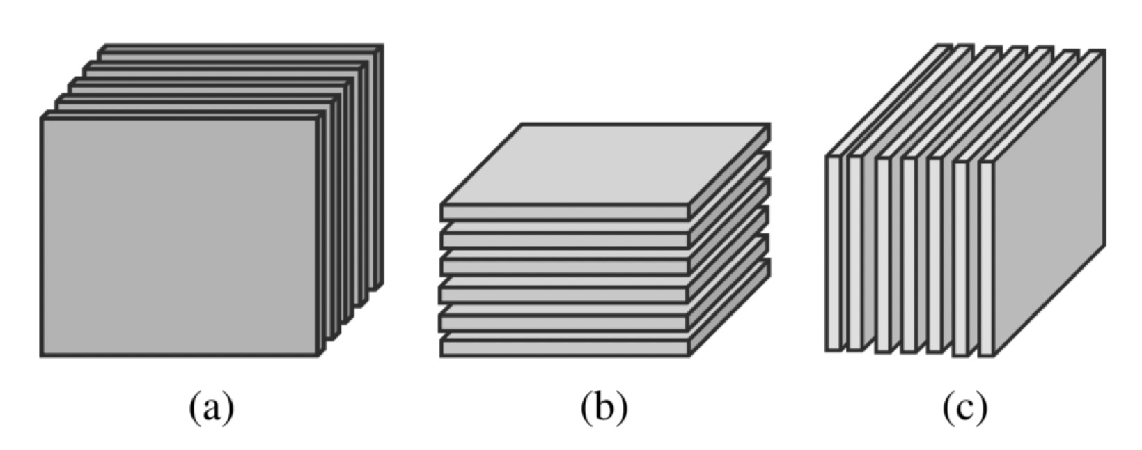
Figure 1: (a) frontal, (b) horizontal, (c) lateral slices of a three order tensor

The frontal slices can be denoted as $A^{(i)}\in\mathbb{R}^{m\times n}$, for convenience. Furthermore, we also define some tensor operators, bcirc, unfold and fold, respectively,

$${\rm bcirc}(\mathcal{A})=\begin{bmatrix}A^{(1)}&A^{(p)}&A^{(p-1)}&\cdots&A^{(2)}\\ A^{(2)}&A^{(1)}&A^{(p)}&\cdots&A^{(3)}\\ A^{(3)}&A^{(2)}&A^{(1)}&\cdots&A^{(4)}\\ \vdots&\ddots&\ddots&\ddots&\vdots\\ A^{(p)}&A^{(p-1)}&A^{(p-2)}&A^{(2)}&A^{(1)}\end{bmatrix}\in\mathbb{R}^{mp\times np},$$

$${\rm unfold}(\mathcal{A}):=\begin{bmatrix}A^{(1)}\\ A^{(2)}\\ \vdots\\ A^{(p)}\\ \end{bmatrix}\in\mathbb{R}^{mp\times n},\quad{\rm fold}({\rm unfold}(\mathcal{A}))=\mathcal{A}.$$

The corresponding inverse operation of bcirc,

$${\rm bcirc}^{-1}:\mathbb{R}^{mp\times np}\rightarrow\mathbb{R}^{m\times n\times p}$$

is defined as

$${\rm bcirc}^{-1}({\rm bcirc}(\mathcal{A}))=\mathcal{A}.$$

2.2 Tensor T-product

Definition 2.1.

(Tensor T-product)

Suppose that there are $\mathcal{A}\in\mathbb{R}^{m\times n\times p}$ and $\mathcal{B}\in\mathbb{R}^{n\times s\times p}$. The T-product between $\mathcal{A}$ and $\mathcal{B}$ is an $m\times s\times p$ tensor defined by

$$\mathcal{A}*\mathcal{B}:={\rm fold}({\rm bcirc}(\mathcal{A}){\rm unfold}(\mathcal{B})).$$

From now on, we will use ‘$*$’ as T-product in the rest of this paper [23].

Definition 2.2.

(Transpose and Conjugate Transpose)

If $\mathcal{A}$ is a third order tensor, whose size is $m\times n\times p$, then the transpose $\mathcal{A}^{\top}$ could be defined from transforming all of the frontal slices and reversing the order of the transposed frontal slices from 2 to $p$. Similarly, the conjugate transpose $\mathcal{A}^{H}$ could also be defined from conjugating all of the frontal slices and reversing the order of the transposed frontal slices from 2 to $p$. Writing these two relationships in MATLAB mathematical forms, we have

$$\begin{cases}\mathcal{A}^{\top}[:,:,0]&=\mathcal{A}[:,:,0]^{\top},\\ \mathcal{A}^{\top}[:,:,i]&=\mathcal{A}[:,:,p-i]^{\top}\ \ {\rm for}\ i=1,2,\ldots,p-1,\\ \mathcal{A}^{H}[:,:,0]&=\mathcal{A}[:,:,0]^{H},\\ \mathcal{A}^{H}[:,:,i]&=\mathcal{A}[:,:,p-i]^{H}\ \ {\rm for}\ i=1,2,\ldots,p-1.\end{cases}$$ (2.2)

Definition 2.3.

(Identity Tensor) The $n\times n\times p$ identity tensor $\mathcal{I}_{nnp}$ is defined as a tensor whose first frontal slice is the $n\times n$ identity matrix, and whose other frontal slices are all zeros.

It is easy to check that for all $\mathcal{A}\in\mathbb{R}^{m\times n\times p}$, there exists $\mathcal{A}*\mathcal{I}_{nnp}=\mathcal{I}_{mmp}*\mathcal{A}=\mathcal{A}$.

Lemma 2.1.

[38] Using the above definitions of T-product and bcirc operator, there exists

(1) $bcirc(\mathcal{A}*\mathcal{B})=bcirc(\mathcal{A})\cdot bcirc(\mathcal{B}),$  (2) $(\mathcal{A}*\mathcal{B})^{H}=\mathcal{B}^{H}*\mathcal{A}^{H}$, $(\mathcal{A}*\mathcal{B})^{\top}=\mathcal{B}^{\top}*\mathcal{A}^{\top}$,

(3) $bcirc(\mathcal{A}^{\top})=bcirc(\mathcal{A})^{\top}$,  $bcirc(\mathcal{A}^{H})=bcirc(\mathcal{A})^{H}$.

It can be easy to notice that the complexity of matrix multiplication to compute T-product by definitions increases rapidly as the dimensions of these tensors goes up, that is $O(mp\times np\times s)=O(mnsp^{2}).$ Fortunately, T-product can be accelerated by the Discrete Fourier Transform (DFT) and the Fast Fourier Transform (FFT). Let $F_{n}$ be the $n\times n$ DFT matrix,

$$F_{n}=\frac{1}{\sqrt{n}}\begin{bmatrix}1&1&1&\cdots&1\\ 1&\omega^{1}&\omega^{2}&\cdots&\omega^{n-1}\\ 1&\omega^{2}&\omega^{4}&\cdots&\omega^{2(n-1)}\\ \vdots&\vdots&\vdots&\ddots&\vdots\\ 1&\omega^{n-1}&\omega^{2(n-1)}&\cdots&\omega^{(n-1)(n-1)}\\ \end{bmatrix},$$

where $\omega=e^{-\frac{2\pi i}{n}}$ is the primitive $n$-th root of unity in which $i^{2}=-1$. It is well-known that a block circulant matrix can be block diagonalized by using the Fourier transform [39],

$${\rm bcirc}(\mathcal{A})=\left(F^{H}_{p}\otimes I_{m}\right)\begin{bmatrix}A_{1}&&&\\ &A_{2}&&\\ &&\ddots&\\ &&&A_{p}\end{bmatrix}\left(F_{p}\otimes I_{n}\right),$$ (2.3)

where $F_{p}^{H}$ is the conjugate transpose of $F_{p}$ and ‘$\otimes$’ is the Kronecker product [40].

2.3 FFT Algorithm to Compute T-product

Following the analysis of Section 2.2, we can generate the algorithm to compute T-product based on the FFT method as follows. By recursively dividing the array into even and odd indexed elements, referring to Subsection 1.4 of [41], the FFT can reduce computational complexity of the DFT. Here we will introduce the well-known FFT algorithm, where $\omega=e^{-\frac{2\pi i}{n}}$ is the primitive $n$-th root of unity and $x(s,t,n)=(x(s),x(s+t),x(s+2t),\ldots,x(s+rt))$ with $x(s+rt)<n\leq x(s+(r+1)t)$.

  Algorithm 1 Fast Fourier Transform Algorithm

 

  $x\in\mathbb{R}^{n}$ and $n=2^{t}$

  the Discrete Fourier Transform of $x$, $\hat{x}=\text{fft}(x,n)$ If $n=1$:     $\hat{x}=x$ Else     $m=n/2$     $d=(1,\omega,\ldots,\omega^{m-1})^{\top}$     $\hat{x}=\left[\begin{matrix}\text{fft}(x(1:2:n),m)+d.*\text{fft}(x(2:2:n),m)\\ \text{fft}(x(1:2:n),m)-d.*\text{fft}(x(2:2:n),m)\end{matrix}\right]$ End

 

In this algorithm, “.*” denotes element-wise multiplication between two vectors. Similarly, inverse Fast Fourier Transform (iFFT) operation can be defined. In [34, 35], Kilmer has shown that (2.3) could be equal to take the DFT and iDFT operation on $\mathcal{A}$ along its third dimension. For $i=1,\ldots,m$ and $j=1,\dots,n$, the tube element vector of $\mathcal{A}\in\mathbb{R}^{m\times n\times p}$ is noted as $\mathcal{A}[i,j,:]$.

  Algorithm 2 T-product Algorithm based on FFT Method

 

  $\mathcal{A}\in\mathbb{R}^{m\times n\times p}$ and $\mathcal{B}\in\mathbb{R}^{n\times s\times p}$

  $\mathcal{C}=\mathcal{A}*\mathcal{B}\in\mathbb{R}^{m\times s\times p}$

Step 1: Take FFT operation on $\mathcal{A}$ For $i=1,\ldots,m$ and $j=1,\dots,n$, $\ \ \ \ \widehat{\mathcal{A}}[i,j,:]$ = fft($\mathcal{A}[i,j,:],$ $p$) End

Step 2: Take FFT operation on $\mathcal{B}$ For $j=1,\ldots,n$ and $t=1,\dots,s$, $\ \ \ \ \widehat{\mathcal{B}}[j,t,:]$ = fft($\mathcal{A}[j,t,:],$ $p$) End

Step 3: Compute the frontal piecewise product between $\mathcal{A}$ and $\mathcal{B}$ For $k=1,\cdots,p$, $\ \ \ \ \widehat{\mathcal{C}}[:,:,k]$ = $\widehat{\mathcal{A}}[:,:,k]\cdot\widehat{\mathcal{B}}[:,:,k]$ End

Step 4: Take iFFT operation on $\mathcal{C}$ For $i=1,\ldots,m$ and $t=1,\dots,s$, $\ \ \ \ {\mathcal{C}}[i,t,:]$ = ifft($\widehat{\mathcal{C}}[i,t,:],$ $p$) End

 

Remark 1.

In this algorithm, the computation complexity is

$$O(m\times n\times s\times p)=O(mnsp).$$

Meanwhile, the cost of FFT in one tube is $O(p\log p)$. So the whole cost of T-product based on FFT method between $\mathcal{A}\in\mathbb{R}^{m\times n\times p}$ and $\mathcal{B}\in\mathbb{R}^{n\times s\times p}$ is

$$O(mnsp+mnp\log p+nsp\log p),$$

which is efficient than just using definition of T-product.

2.4 Reviews of Tensor Deep Learning Methods

As a high-order data storage structure, tensor has the property of preserving structures and connections among different data points. On contrary, vectorization always destroys the data structure, which might limit the performance of model. In plenty of deep learning tasks, such as color images, video, and a variety of time-varying signals, tensors have obvious advantages. At the same time, the nonlinearity and flexibility implied by the tensor operator offer more freedom to the model construction. There has been a lot of research on tensor deep learning to propose many important ideas and models. For instance, in [42], Shi, Ma, and Fu propose a fuzzy support tensor product method for image classification, utilizing lots of unlabeled image data and improving the network robustness. Meanwhile, in [43], Naumov et al. uses Tetra-AML toolbox and tensor network to provide model compression for deep network like ResNet-18. In addition to some traditional senses, the tensor network also makes improvement in medical image classification [44] and quantum-based image recognition [45, 46]. Apart from RGB images, tensor neural networks have many applications in hyperspectral image (HSI) image recognition. A tensor-based dictionary self-taught learning classification method is proposed for solving precise object classification problems based on Hyperspectral imagery with limited training data [47]. Besides, in [48], Liu, Ma, and Wang studied HSI and intuitively represented HSI as a third-order tensor. In the sparse tensor dictionary learning algorithm, the joint spatial-spectral information can significantly improve the accuracy of HSI classification, combining with tensor Turker decomposition [49, 50]. Meanwhile, different from the traditional vector-based or matrix-based methods, in [51], tensor technique is adopted to extract the joint spatial-spectral tensor features. Tensor T-product [23] is also studied to model the forward propagation in neural networks. Besides, some other researches focus on tensor deep learning modeling [52, 53, 54, 55].

3 Adaptive Data Augmentation Framework

In this section, the Adaptive Data Augmentation Framework based on T-product will be derived and the Tensor Back-Propagation algorithm will be introduced.

3.1 Adaptive Data Augmentation Framework based on Tensor T-product

In such a $K$-classification image recognition task, there is a model, $\mathcal{F}$, that needs to be improved. Assume that the parameter space of this model is $\Phi$. The $i$-th image data is considered in RGB (Red, Green, Blue) as a three-order tensor $\mathcal{A}^{(i)}\in\mathbb{R}^{m\times n\times 3}$.

Following this, the label of observed data $\mathcal{A}^{(i)}$ which belongs to $k$-th class is a $k$-dimension one-hot vector $\bm{y}_{i}$, where

$$y_{ij}=\begin{cases}1,\ \ \ j=k,\\ 0,\ \ \ j\neq k.\end{cases}$$

Then our goal is to make sure that

$$k=\arg\max\mathcal{F}(\mathcal{A}^{(i)};\Phi),$$ (3.1)

where $\mathcal{F}(\mathcal{A}^{(i)};\Phi)$ is also a $k$-dimension prediction vector, $p_{i}=\mathcal{F}(\mathcal{A}^{(i)};\Phi).$

There are many kinds of loss function that we could choose. In this paper, what we utilize is Cross Entropy function,

$$\mathcal{L}=-\frac{1}{N}\sum_{i}\sum_{k=1}^{K}y_{ik}\log(p_{ik}),$$ (3.2)

where $y_{ik}$ is the label of data $i$ and $p_{ik}$ is the predicted probability that the observed sample $i$ belongs to the class $k$.

As we introduce about the T-product, if we permute a image data $\mathcal{A}_{0}\in\mathbb{R}^{m\times n\times 3}$ into ${\mathcal{A}}_{1}\in\mathbb{R}^{m\times 3\times n}$ and ${\mathcal{A}}_{2}\in\mathbb{R}^{n\times 3\times m}$, the parameter tensors, $\mathcal{W}_{1}\in\mathbb{R}^{3\times 3\times n}$ and $\mathcal{W}_{2}\in\mathbb{R}^{3\times 3\times m}$, could be multiplied to maintain the size of the permuted image tensor data. The sizes of

$$\mathcal{A}_{1}*\mathcal{W}_{1}\in\mathbb{R}^{m\times 3\times n}$$

and

$$\mathcal{A}_{2}*\mathcal{W}_{2}\in\mathbb{R}^{n\times 3\times m}$$

are both similar to those of $\mathcal{A}_{1}$ and $\mathcal{A}_{2}$. The following figure can help readers understand the process better.

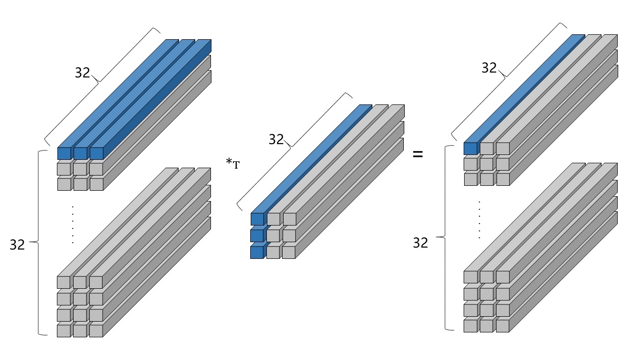
Figure 2: Tensor T-Product in T-ADAF between $\mathcal{A}_{i}\in\mathbb{R}^{32\times 3\times 32}$ and $\mathcal{W}_{i}\in\mathbb{R}^{3\times 3\times 32},\ i=1,2$

The blue tubes in the above Figure shows how FFT and dot product work in T-product. All of the data can be permuted into a normal image size $\mathbb{R}^{m\times n\times 3}$. As a consequence, they can be treated as two new images and taken into the processing of classification. From the model, $\mathcal{F}$, three results can be gained, $\bm{r}=(r_{0},r_{1},r_{2})^{\top}$,

$$\begin{cases}r_{0}&=\mathcal{F}(\mathcal{A}_{0};\Phi),\\ r_{1}&=\mathcal{F}(\mathcal{A}_{1};\Phi),\\ r_{2}&=\mathcal{F}(\mathcal{A}_{2};\Phi).\end{cases}$$ (3.3)

These three results are combined together to gain the final prediction result

$$r=\bm{w}^{\top}\bm{r}=w_{0}r_{0}+w_{1}r_{1}+w_{2}r_{2},$$ (3.4)

where $\bm{w}=(w_{0},w_{1},w_{2})^{\top}$ is the corresponding weight of each results.

Remark 2.

It should be noticed that:

• T-product could be considered as the projections into different dimensions and the weights show the importance of these corresponding projections.

• The weights $w_{i}$, $i=0,1,2$ could be chosen as any vectors, which satisfy

  $$w_{0}+w_{1}+w_{2}=1,$$ (3.5)

  such as $\left(\frac{1}{3},\frac{1}{3},\frac{1}{3}\right)$, $\left(\frac{1}{2},\frac{1}{4},\frac{1}{4}\right)$ or $(\frac{2}{5},\frac{3}{10},\frac{3}{10})$.

• The weights in T-product, $\mathcal{W}_{i},\ i=1,2$ are all initialized by identity tensor on T-product, $\mathcal{I}_{nnp},$ to make sure that

  $$\mathcal{F}(\mathcal{A}_{0};\Phi)=\mathcal{F}(\mathcal{A}_{1};\Phi)=\mathcal{F}(\mathcal{A}_{2};\Phi).$$

  Moreover, considering T-ADAF as a functional on the model function space $\mathscr{F}=\{\mathcal{F}\}$ and noting it as $\Theta$, there exists that

  $$\Theta(\mathcal{F}|\Phi^{(0)},\mathcal{W}_{1}^{(0)},\mathcal{W}_{2}^{(0)})=\mathcal{F}(\ \cdot\ |\Phi^{(0)}),\ \ for\ \mathcal{F}\in\mathscr{F},$$

  where $\Phi^{(0)},\mathcal{W}_{1}^{(0)},\mathcal{W}_{2}^{(0)}$ are the initial parameters of original model and T-product, respectively.

Figure 3: Model Enhancement Framework based on T-product

For convenience, Figure 3 is the schematic illustration of the framework based on T-product. In the full of framework, all of the hyper-parameters when training are maintained, such as learning rates, batch size, etc.

3.2 Tensor Back-Propagation based on T-product

In this subsection, Tensor Back-Propagation (BP) [56, 57] based on T-product will be introduced. If an algorithm engineer could rewrite the BP algorithm in Cuda or Pytorch, it will save some time to train the neural network with our Adaptive Data Augmentation Framework. These conclusion has been derived by Newman et al. [23, Derivation 4.1].

Theorem 3.1.

Suppose that forward propagation of tensor T-product operation in a neural network is

$$\mathcal{A}_{j+1}=\sigma(\mathcal{Z}_{j+1})=\sigma(\mathcal{W}_{j}*\mathcal{A}_{j}+\mathcal{B}_{j}),$$ (3.6)

for $j=0,1,\ldots,N$, where $\sigma(\cdot)$ is the activation function. $\mathcal{M}$ is the whole tensor neural network. Then the tensor back-propagation formulas can be computed by,

$$\delta\mathcal{A}_{N}=\mathcal{W}_{N}^{\top}*\frac{\partial\mathcal{M}}{\partial\mathcal{A}_{N}},$$ (3.7)

$$\delta\mathcal{A}_{j}=\mathcal{W}_{j}^{\top}*(\delta\mathcal{A}_{j+1}\odot\sigma^{\prime}(\mathcal{Z}_{j+1})),\ \ {\rm for}\ \ i=0,1,\ldots,N-1,$$ (3.8)

$$\delta\mathcal{W}_{j}=(\delta\mathcal{A}_{j+1}\odot\sigma^{\prime}(\mathcal{Z}_{j+1}))*\mathcal{A}_{j}^{\top},\ \ {\rm for}\ \ i=0,1,\ldots,N-1,$$ (3.9)

where

$$\delta\mathcal{A}_{j}:=\frac{\partial\mathcal{M}}{\partial\mathcal{A}_{j}},\ \ {\rm for}\ \ i=0,1,\ldots,N,$$

is the erros on the $j$-th layer, $\delta^{\prime}$ is the derivative of the activation function and ‘$\odot$’ is the Hadamard element-wise product.

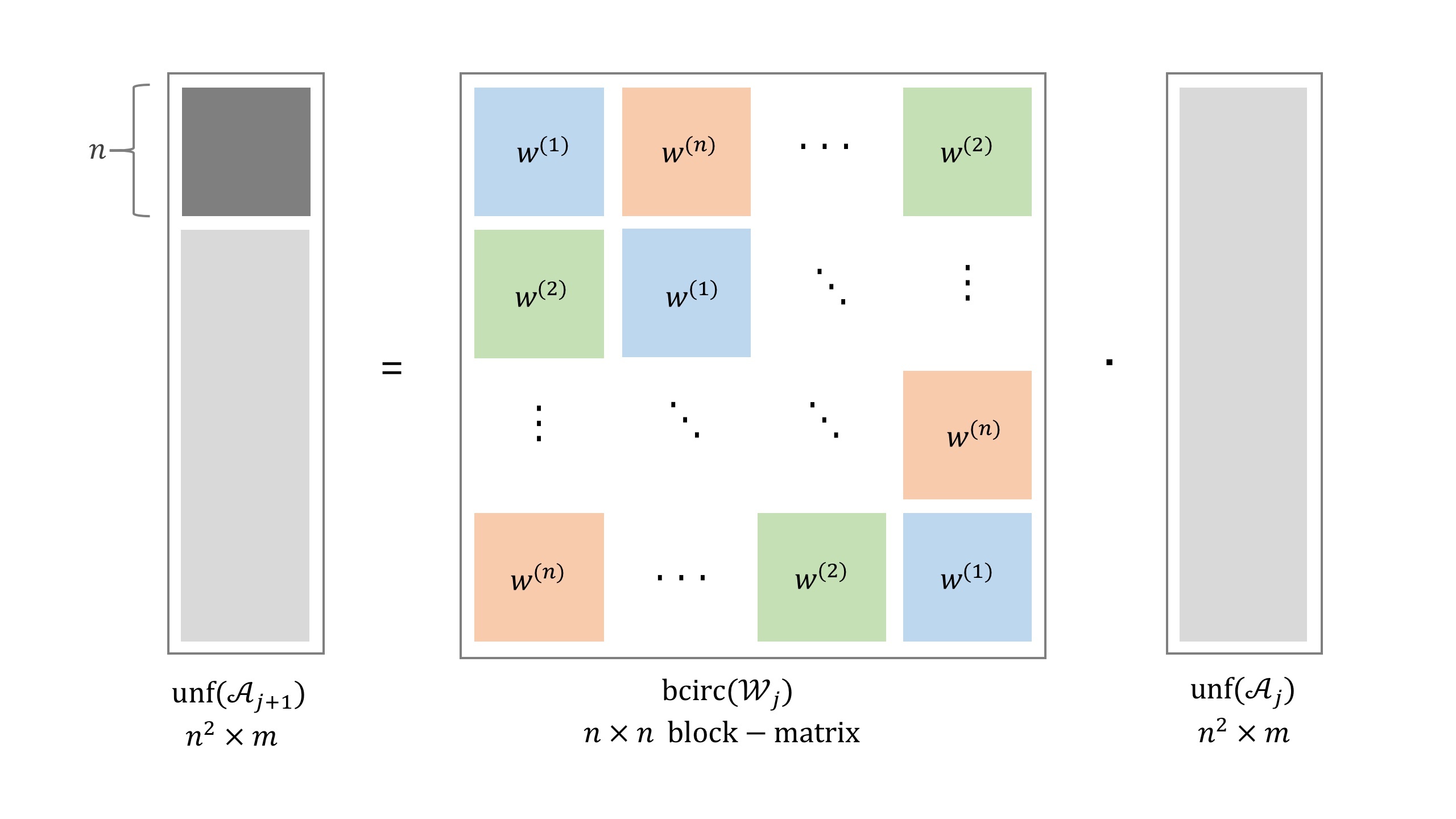
Figure 4: Definition of Tensor T-Product with Bcirc Operator

Suppose that the auto back-propagation operator in PyTorch or TensorFlow is noted as $\Psi(\delta_{final};\mathcal{F})$, where $\mathcal{F}$ is the original model and $\delta_{final}$ is the error in the final step between the actual target vector and final predicted result. From the above definition,

$$\Psi(\delta_{final};\mathcal{F})=\delta_{T},$$ (3.10)

where $\delta_{T}$ is the error after T-product.

  Algorithm 3 Back-Propagation Algorithm for T-ADAF

 

  The final error between the actual target vector and final predicted result, $\delta_{final}$. The original model, $\mathcal{F}$. Initial data before T-product, $\mathcal{A}_{0}\in\mathbb{R}^{m\times n\times 3}$.

  The error of weights in T-product, $\delta\mathcal{W}_{0}$.

Hyper-parameters: The batch size, $B$. The maximum number of iteration epochs, $N$. The learning rate schedule, $\eta_{i},\ i=1,\ldots,N.$ The optimizer to train the model parameters, $\mathcal{O}$. The weights of each prediction results, $w$. Initial weights in T-product, $\mathcal{W}_{0}\in\mathbb{R}^{3\times 3\times n}$.

Step 1: Compute the error after T-product, $\delta_{T}$, using the auto back-propagation operator in PyTorch,

$$\Psi(\delta_{final};\mathcal{F})=\delta_{T}.$$

Step 2: Permute $\delta_{T}\in\mathbb{R}^{m\times n\times 3}$ into $\widehat{\delta}_{T}\in\mathbb{R}^{m\times 3\times n}$ and $\mathcal{A}_{0}\in\mathbb{R}^{m\times n\times 3}$ into $\widehat{\mathcal{A}_{0}}\in\mathbb{R}^{m\times 3\times n}$.

Step 3: Compute the permuted error of weights in T-product, ${\delta\mathcal{W}_{0}}^{\top}$.

    Step 3.1: Compute

$$\widehat{\delta\mathcal{A}_{0}}^{\top}=\mathcal{W}_{0}*\left(\widehat{\delta}_{T}^{\top}\odot\sigma^{\prime}\left(\mathcal{W}_{0}^{\top}*\widehat{\mathcal{A}_{0}}^{\top}\right)\right).$$

    Step 3.2: Compute

$${\delta\mathcal{W}_{0}}^{\top}=\left(\widehat{\delta}_{T}^{\top}\odot\sigma^{\prime}\left(\mathcal{W}_{0}^{\top}*\widehat{\mathcal{A}_{0}}^{\top}\right)\right)*\mathcal{A}_{0}.$$

Step 4: Permute ${\delta\mathcal{W}_{0}}^{\top}\in\mathbb{R}^{3\times 3\times n}$ into ${\delta\mathcal{W}_{0}}\in\mathbb{R}^{3\times 3\times n}$.

 

Remark 3.

Compared with the original automatic back propagation algorithm in PyTorch Toolbox, Algorithm 3 does not need to calculate the numerical difference of T-product operator. Therefore, Algorithm 3 avoids multiple computations of the entire frame map and reduces the consumption of calculation.

3.3 Analysis of T-ADAF

According to the definition of T-product, such a circulant convolution-like structure will extract a more comprehensive global data feature information for any side of it. For each frontal slice, the T-product

$$\mathcal{C}=\mathcal{A}*\mathcal{B}$$ (3.11)

could be considered as a circulant convolution-like structure,

$$C^{(k)}=A^{(k)}\cdot B^{(1)}+\sum_{i=1}^{k-1}A^{(i)}\cdot B^{(k-i+1)}+\sum_{i=k+1}^{n}A^{(i)}\cdot B^{(n-i+k+1)},$$ (3.12)

for $k=1,2,\ldots,n$.

There may be some connections between two blocks of pixels that are far apart and can provide valuable information for model prediction. However, only with the local convolution and pooling operations of the neural network, such features may be diluted or even disappeared. But T-product provides the ability to obtain more global information.

In T-ADAF, T-product plays the role of frequency domain information extraction and analysis. Let us review the algorithm to compute T-product between two tensors,

$$\mathcal{A}*\mathcal{W}=iDFT(DFT(\mathcal{A})\star DFT(\mathcal{W})),$$ (3.13)

where ‘$\star$’ means the slice-wise dot product, i.e.,

$$\mathcal{A}\star\mathcal{W}[:,\ :,\ i]=\mathcal{A}[:,\ :,\ i]\ \mathcal{W}[:,\ :,\ i],$$ (3.14)

for $i=1,2,\ldots,N$. DFT transforms image data from spatial domain to frequency domain. Then the linear mapping can be understood as a fully connected layer to extract and analyze the frequency domain signals. Finally, iDFT transfers the data from the frequency domain back to the spatial domain. As a consequence, the data generated through this series of processes are provided to the neural network for further learning as the result of data augmentation, thus improving the performance of original model.

4 Numerical Results

In this section, we aim to make the numerical experiences as close as possible to the actual applications and illuminate that the improvements derive from the T-product-based framework indeed. For these purposes, we present the numerical results in the order by the time when the original models were published. We divide the numerical experiments into two parts, LeNet-5 models and Deep Neural Network models. Looking back on the history of neural networks, LeNet-5 was proposed and studied early. With introduction of deeper models, LeNet-5 gradually faded out of the limelight. However, for many application scenarios, it still has the advantages of smaller memory consumption and fast training speed. For some projects that do not require too high prediction accuracy, small models are a less expensive option. In the past decade, many neural network models with sophisticated design and high performance have been proposed, which we classify as deeper models and explore the effectiveness of this data augmentation framework for these models. We have tested the framework in some undisclosed data sets with some success. In this section, we present the numerical results based on open data sets.

4.1 Preparations and Hyper-parameter Settings

The CIFAR-10 dataset consists of $32\times 32\times 3$ RGB images belonging to $10$ different classes, 50,000 training images and 10,000 testing images. Meanwhile, CIFAR-100 dataset consists of $32\times 32\times 3$ RGB images belonging to $100$ different classes, 50,000 training images and 10,000 testing images. Each set of images is equally distributed among different classes. We normalize the (R, G, B) channels of each image with means of $(0.4914,0.4822,0.4465)$ and standard deviations of $(0.2023,0.1994,0.2010)$.

The batch size, $B$, is set as 32. The maximum number of iteration epochs, $N$, is 100 for LeNet-5, while $N=200$ for other models. The optimizer to train the model parameters is Adam [58]. The weights in T-product, $\mathcal{W}_{0}\in\mathbb{R}^{3\times 3\times n}$, is initialized as $\mathcal{W}_{0}=\mathcal{I}$, since we want the data augmentation is started from the situation without any changes, i.e., $\mathcal{A}*\mathcal{I}=\mathcal{A}$. As for the learning rate schedules, $\eta_{i},\ i=1,\ldots,N,$ they are also different for each cases. The learning rates of tensor product parameters are one fifth of those of deep learning network parameters. For reproducing the original performance in [59], the learning rate schedule of CCT / CVT remains unchanged, with the learning rate nonlinear declining. The learning rate schedules of LeNet-5, VGG, ResNet, and MobileNet with T-ADAF are listed in Table 1 and Table 2.

Epoch	1-50	51-100
LeNet-5	0.1	0.02
T-product	0.02	0.004

Table 1: Learning Rate Schedule of LeNet-5 with T-ADAF

Epoch	1-60	61-120	121 - 160	161-200
VGG / ResNet / MobileNet	0.1	0.02	0.004	0.0008
T-product	0.02	0.004	0.0008	0.00016

Table 2: Learning Rate Schedule of VGG, ResNet and MobileNet with T-ADAF

	$w_{0}$	$w_{1}$	$w_{2}$
333	$\frac{1}{3}$	$\frac{1}{3}$	$\frac{1}{3}$
433	0.4	0.3	0.3
525	0.5	0.25	0.25

Table 3: Suffixes of the model name and their meanings

Here, $w_{0}$ is the wight of the original image. Essentially these parameters indicate how important the original image is relative to the other two images.

4.2 Numerical Results of LeNet-5 with T-ADAF

In practical applications, especially with computational power and storage space limited, LeNet-5 is also an available model. This model, from the paper [60], is an old but very efficient convolutional neural network for handwritten character recognition. Meanwhile, algorithm scientists usually do not pursue an accuracy improvement of less than one percentage point, but are more concerned with reducing training costs. In order to better simulate the model evaluation metric in practical applications, two new definitions are introduced here.

Definition 4.1.

For any single trained model $\mathcal{F}$, assume that its iteration sequence is $\{t\in\mathbb{N}^{+}:1\leq t\leq T\}$, where $T$ is the maximum number of iterations. The corresponding training iteration parameter sequence is $\left\{\mathcal{W}_{t}\right\}_{1\leq t\leq T}$. Let $\left\{\lambda_{t}\right\}_{1\leq t\leq T}$ be the sequence of accuracy rates in the iterative process. Then the minimum available number of training iterations for the model $\mathcal{F}$ in this training iteration is defined as,

$$t^{ava}=\operatorname*{argmin}_{1\leq t\leq T}\left\{\lambda_{t}\geq\lfloor\lambda_{\max}\rfloor\right\},$$

where $\lfloor\cdot\rfloor$ means the round down operation and

$$\lambda_{\max}=\max_{1\leq t\leq T}\{\lambda_{t}\}.$$

Meanwhile, the available accuracy rate is

$$\lambda_{\min}^{ava}=\lfloor\lambda_{\max}\rfloor$$

Definition 4.2.

A trained model group $\mathcal{G}$ contains one original model $\mathcal{F}_{0}$ and some other enhanced model $\mathcal{F}_{i},i=1,2,\ldots,m$. Assume that their iteration sequences are $\{t\in\mathbb{N}^{+}:1\leq t\leq T\}$, where $T$ is the maximum number of iterations. Let $\left\{\lambda_{t}^{(i)}\right\}_{1\leq t\leq T},i=0,1,\ldots,m,$ be the sequences of accuracy rates in these iterative processes. From Definition 4.1, the minimum available number of training iterations for the group $\mathcal{G}$ is defined as

$$t^{ava}_{i}=\operatorname*{argmin}_{1\leq t\leq T}\left\{\lambda_{t}^{(i)}\geq\lfloor\lambda_{\max}^{(0)}\rfloor\right\}.$$

for $i=1,2,\ldots,m$.

Here, we mainly test the performance of LeNet-5 on CIFAR-10 and CIFAR-100. The only thing to note is that LeNet-5 was originally designed to process greyscale images, while CIFAR10 and CIFAR100 are both RGB images. Therefore, we need to modify the parameters of the convolution kernel to make LeNet-5 meet our experimental requirements.

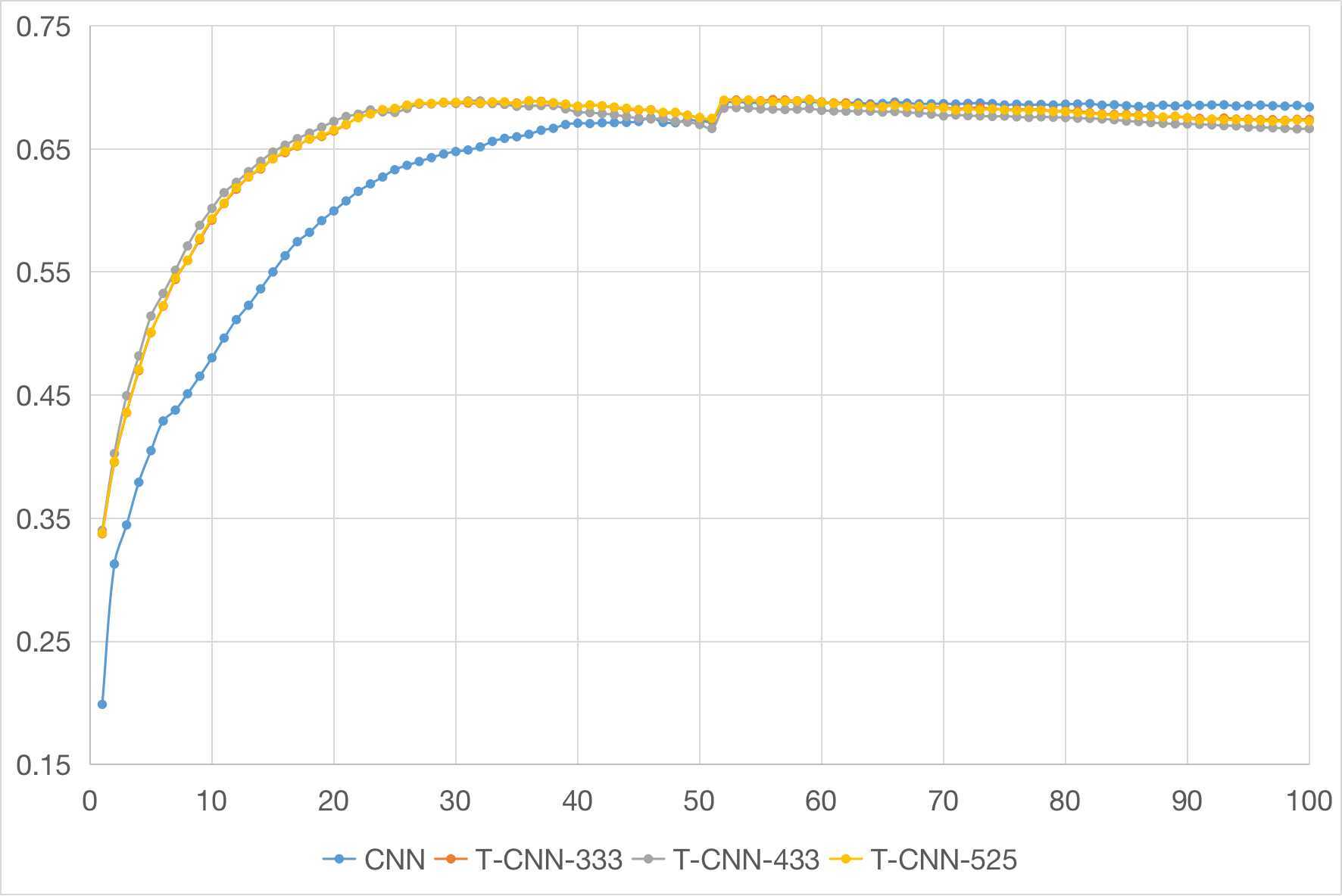
(a) CIFAR-10

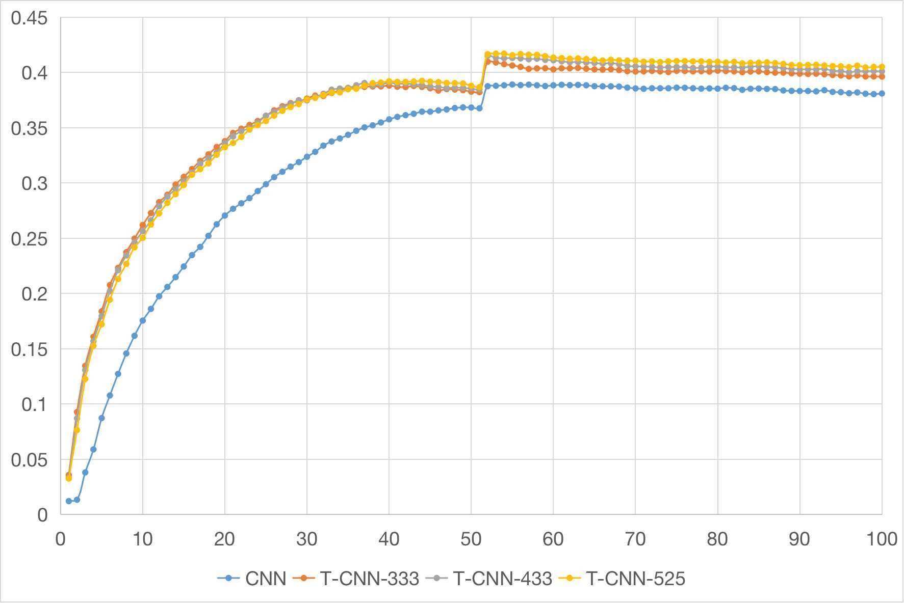
(b) CIFAR-100

Figure 5: LeNet-5 Model with T-product Enhancement Framework

In the Figure 5, we can see that for the CIFAR-100 dataset, the data augmentation framework can not only accelerate the iterative convergence speed of the deep learning model, but also improve the prediction accuracy of the original model. For the CIFAR-10 dataset, each category has 5000 samples to be learned, so the effect of final prediction accuracy enhancement is not obvious. But the data augmentation framework still reduces the number of iterations required. From Definition 4.2, we summarize the whole iteration processes as Table 5.

	$\lambda_{\max}^{(0)}$	$\lfloor\lambda_{\max}^{(0)}\rfloor$	$\lambda_{\max}^{(T333)}$	$\lambda_{\max}^{(T433)}$	$\lambda_{\max}^{(T525)}$
CIFAR-10	0.6888	0.68	0.6876	0.6886	0.6898
CIFAR-100	0.3859	0.38	0.4066	0.4118	0.4137

Table 4: Maximum Accuracy Rates of Numerical Results when Testing LeNet-5

	Original	T333	T433	T525
CIFAR-10	52	24	24	25
CIFAR-100	52	34	33	35

Table 5: Minimum Epochs to Attend $\lfloor\lambda_{\max}^{(0)}\rfloor$ when Testing LeNet-5

Among them, T433 represents the model that uses the T-product to enhance the framework and takes 0.4-0.3-0.3 as the weights. As it can be seen from Table 4 and Table 5, since the amount of data in the CIFAR-10 dataset is relatively sufficient, the advantages of the data enhancement framework are not obvious, and the effect of CIFAR-100 is more obvious. However, for both datasets, there is a clear advantage to reaching the minimum number of iterations available. This shows that in practical applications, a model using the data augmentation framework can be trained into use in fewer iteration steps.

4.3 Numerical Results of Deep Neural Network with T-ADAF

In this subsection, we test four models, VGG-16, ResNet-18, ResNet-34 and CCT-6, respectively. Due to the relatively high complexity and information extraction ability of these four models, the ten-category problem of the CIFAR-10 dataset is not challenging for them. The test accuracy rate has reached more than 95%, even 98%. Therefore, to better illustrate the performance of the adaptive data augmentation framework, we only show and analyze the performance of these four models.

VGG-Net, first proposed in 2014, have proved that increasing the depth of the network can affect the final performance of the network. In VGG, multiple small convolution kernels are used instead of a large convolution kernel that had been commonly used before to reduce the calculation amount of convolution operations under the condition of ensuring the same receptive field. VGG-Net increases the depth of network and improves the effect of that. ResNet, which was first proposed in 2015 [61], used the residual structure in the neural network model for the first time, which solved the problem of gradient disappearance that often occurred when the number of layers in the previous model was increased. Since then, deep neural networks have become truly possible, and deep learning has gained more and more attention. Empirically, the depth of the network is critical to the performance of the model. When the number of network layers is increasing, the network can extract more complex feature patterns, so theoretically better results can be achieved. ResNet has gained good results in various competitions that year. Moreover, transformer [62] was a common model in the field of natural language processing and was introduced in Computational Vision in 2018. Vision transformer (ViT) achieves further improvements in prediction performance by stacking attention modules [14]. CCT [59] reduces the number of parameters on the premise of ensuring the prediction accuracy, and provides convenience for the application and promotion of ViT.

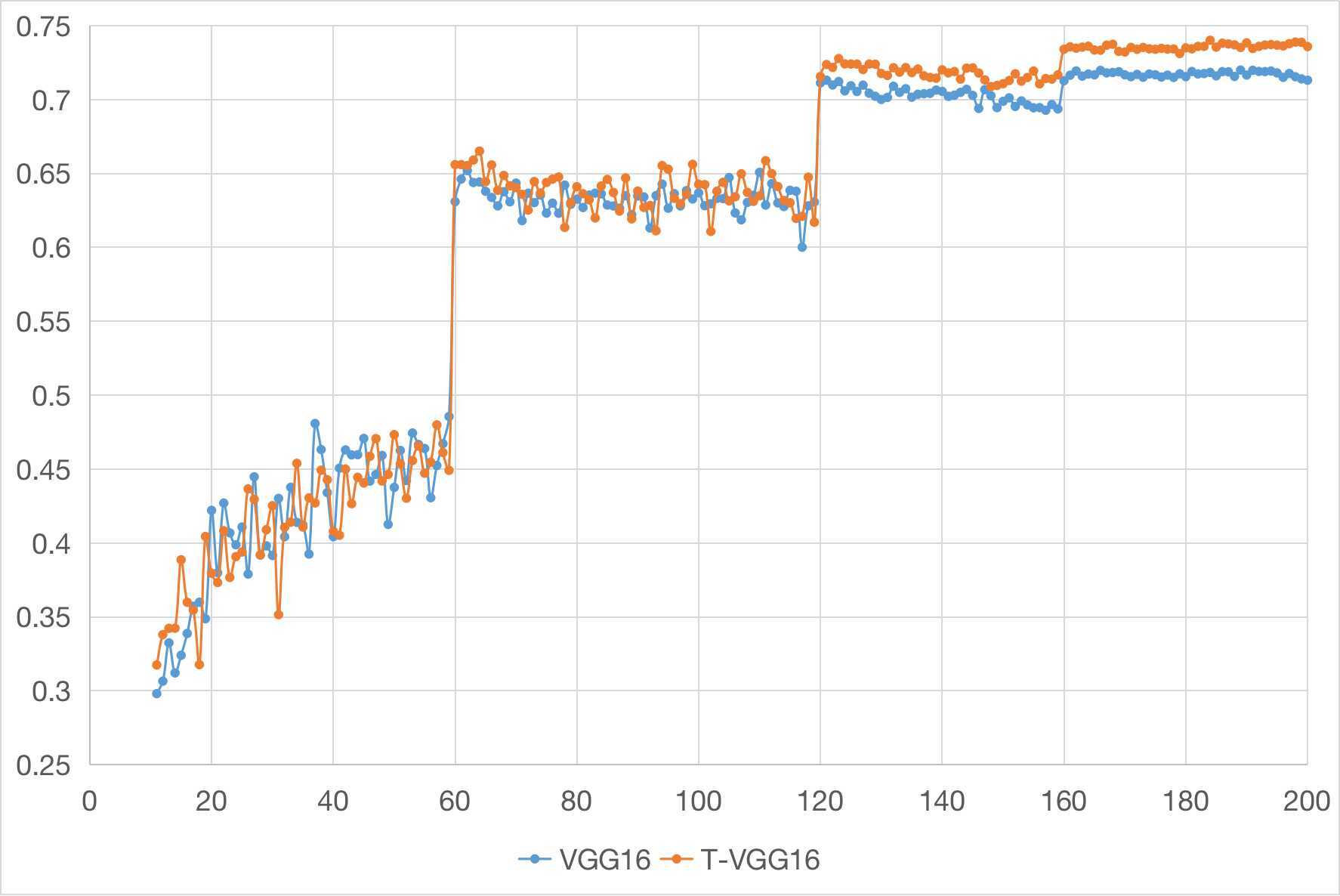
(a) Epoch 10-200

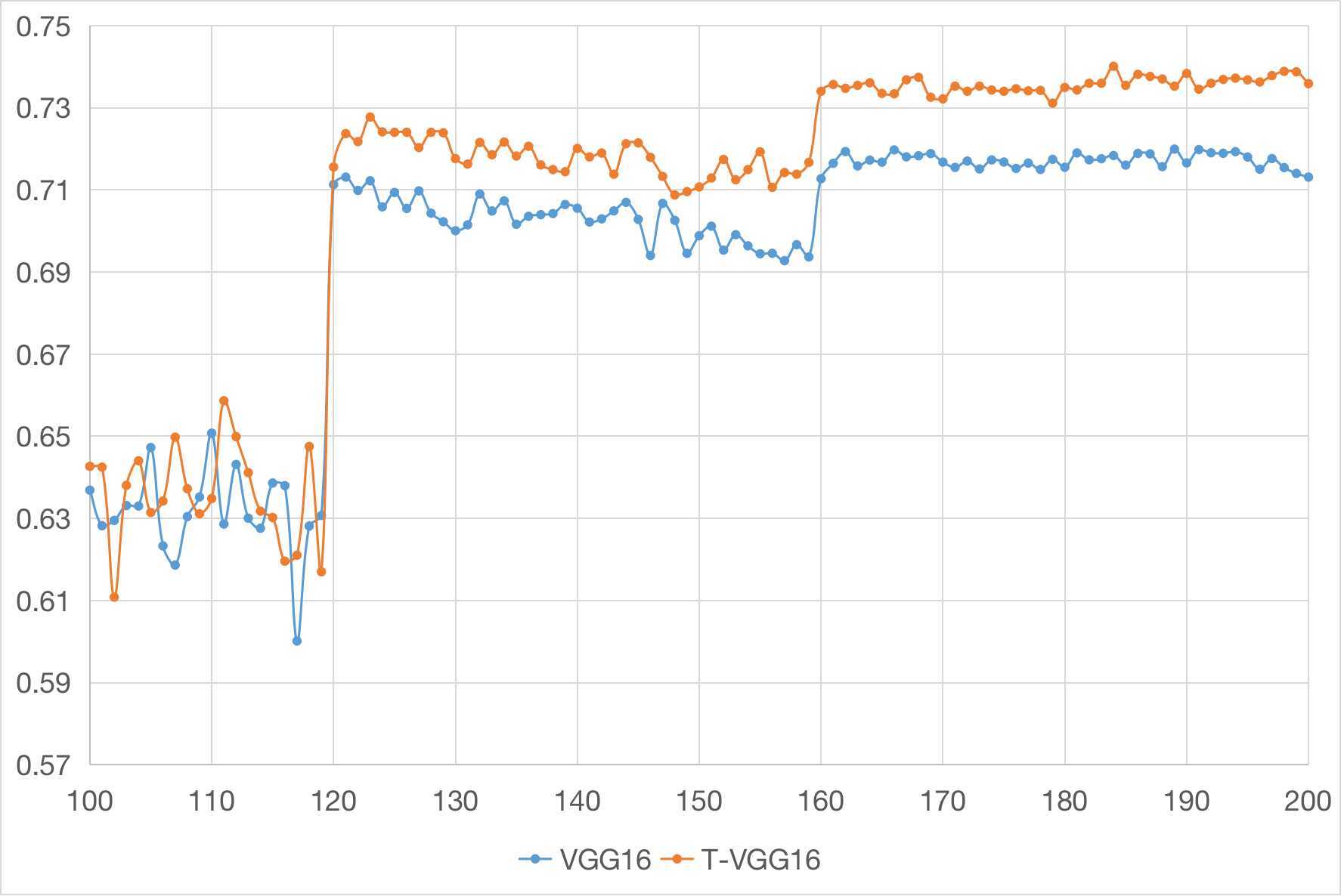
(b) Epoch 100-200

Figure 6: VGG-16 Model with T-ADAF

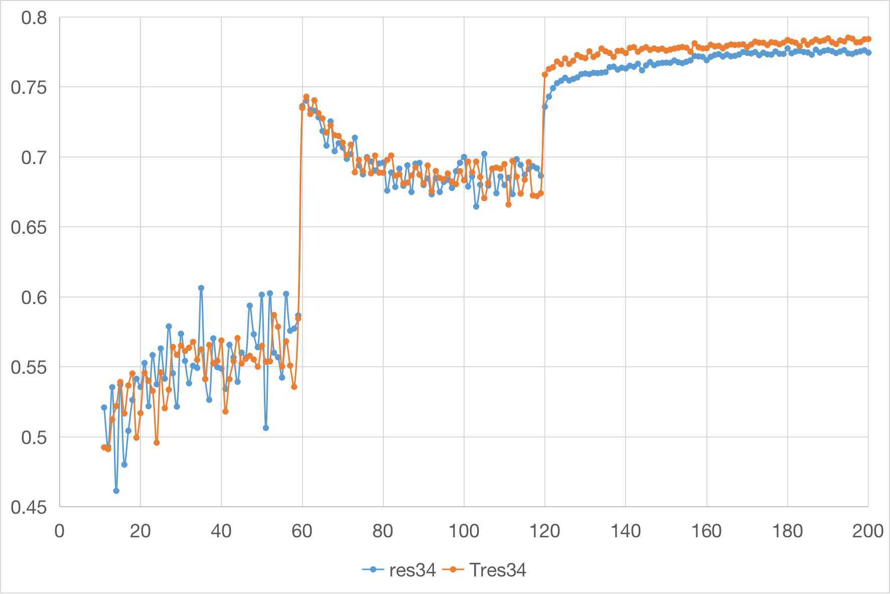
(a) Epoch 10-200

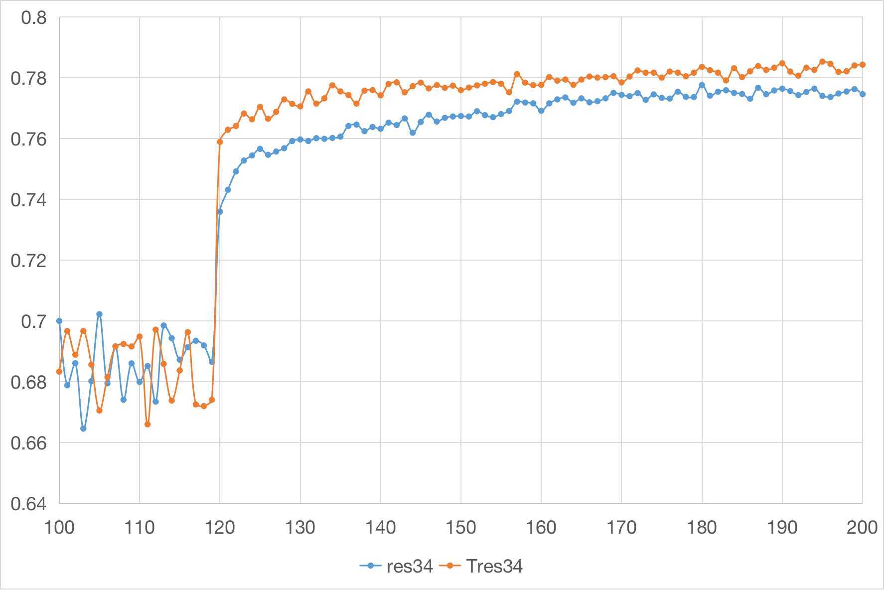
(b) Epoch 100-200

Figure 7: ResNet-34 Model with T-ADAF

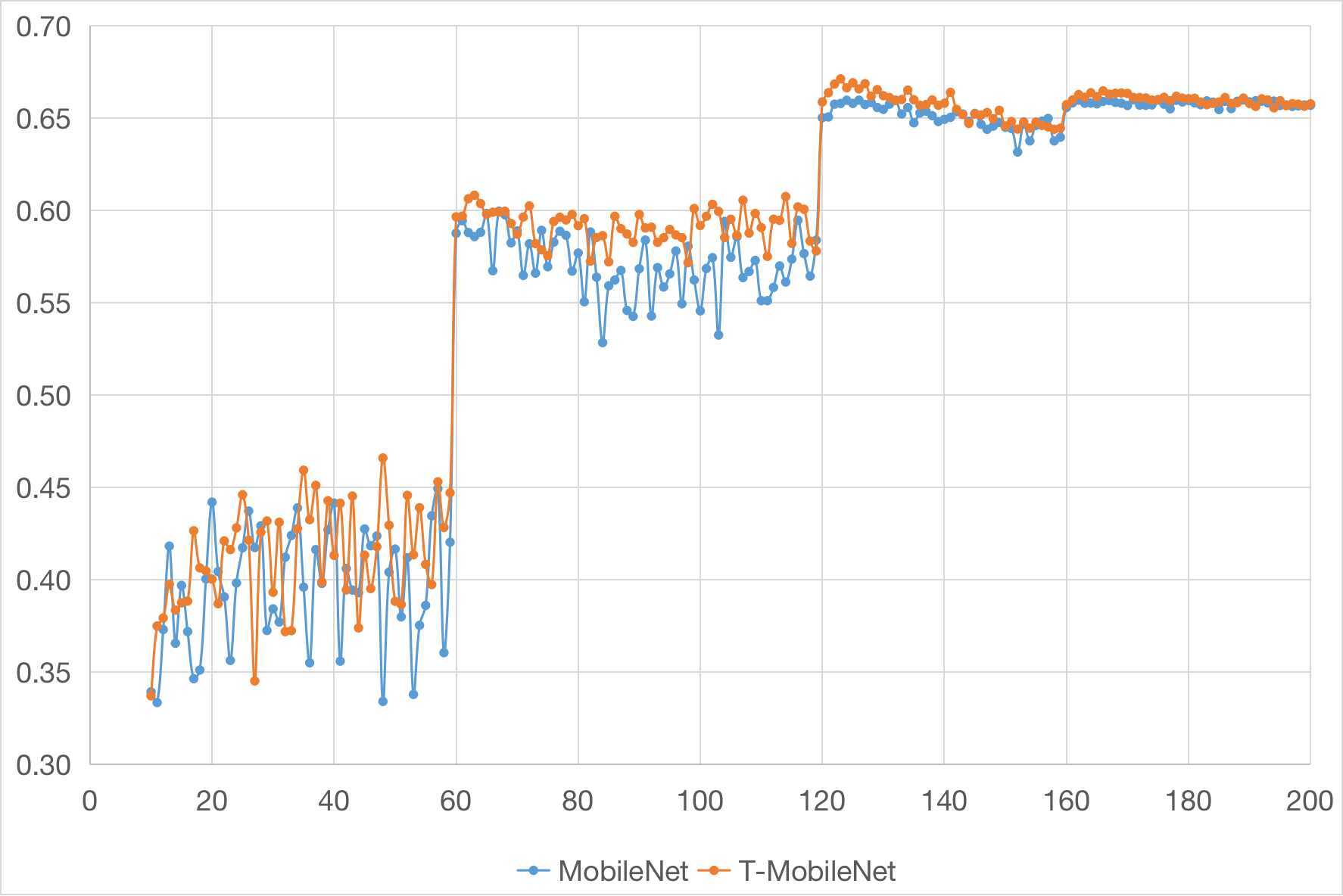
(a) Epoch 10-200

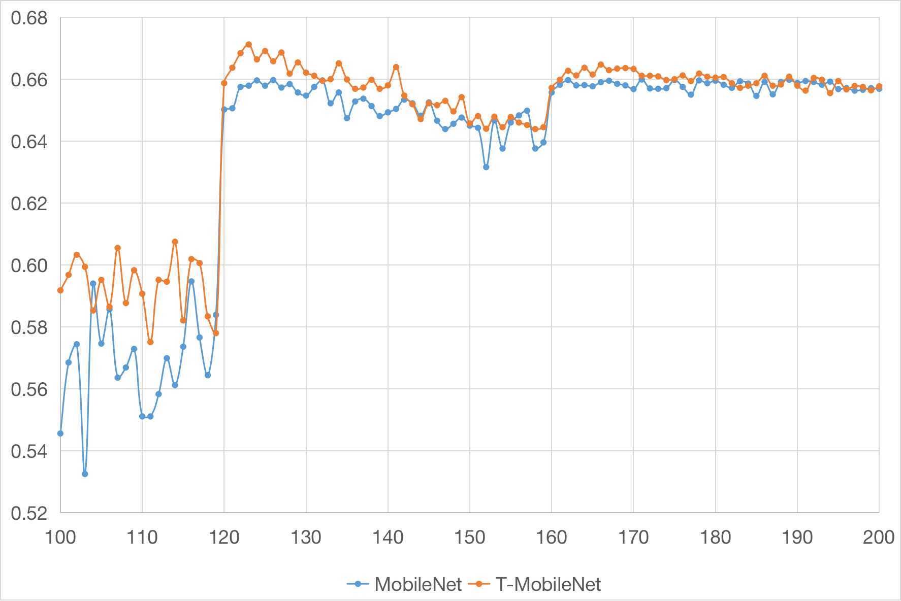
(b) Epoch 100-200

Figure 8: MobileNet Model with T-ADAF

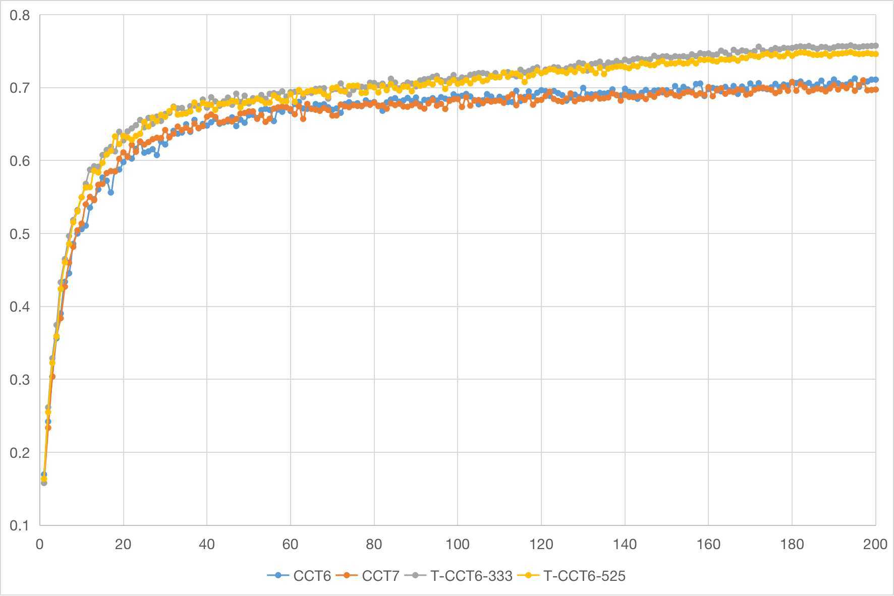
Figure 9: CCT-6 Model with T-ADAF about Top-1 Accuracy on CIFAR-100

Figure 6-8 show how the prediction accuracy changes with the iterative epoch increasing. For convenience, we separately show the process of epoch 100-200 in the (b) picture. We choose VGG-16, ResNet-34 and CCT-6 as examples for showing iteration details.

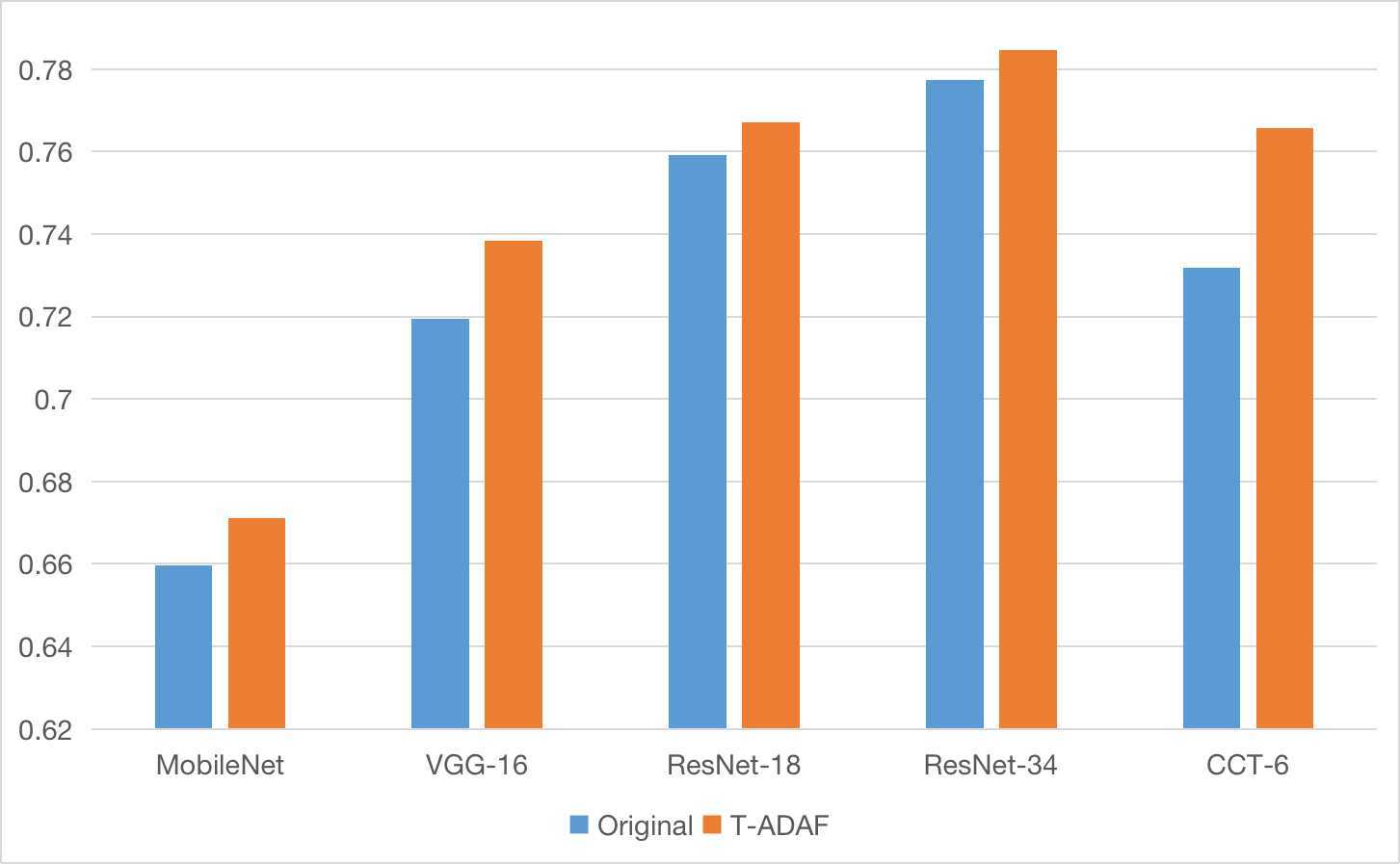
Figure 10: Comparisons among 5 Different Models and T-ADAF

Model		Original	T-333	T-433	T-525
VGG-16	Top-1	0.2805	0.2726	0.2674	0.2616
	Top-5	0.1061	0.0924	0.0921	0.0915
ResNet-18	Top-1	0.2409	0.2356	0.2330	0.2361
	Top-5	0.0725	0.0648	0.0616	0.0652
ResNet-34	Top-1	0.2226	0.2194	0.2153	0.2171
	Top-5	0.0601	0.0575	0.0558	0.0569
CCT-6	Top-1	0.2681	0.2342	0.2393	0.2405
	Top-5	0.0728	0.0621	0.0673	0.0714

Table 6: Errors of Numerical Results for Testing Deep Models on CIFAR-100

From these results, we can see that the data augmentation framework can indeed improve the performance and fasten accelerate learning iteration speed of the model. The data augmentation frameworks under different weight settings are slightly different, but generally all perform better than the original models.

Remark:

• In the adaptive data augmentation framework based on tensor T-product, the parameters in T-product in epoch 1-120 are learnable, while the T-product parameters are designed to remain unchanged in epochs 121-200. In addition, we have tested to find that fixing T-product parameter in epochs 121-200 does not affect the model performance and could avoid the risks of over-fitting.

• Numerical experiments are based on Intel i5-10400F with NVIDIA 3080-10G. In the first 120 epochs, the running time of the enhanced model is about 4.5 times of that of the original model. Among them, the time consumption caused by data augmentation is three times, and the extra consumption caused by T-product operator is about 1.5 times of that of the original model. Meanwhile, in epochs 121-200, the enhanced model costs 2.2 times more time than the original model.

4.4 Comparisons with Tensor Neural Network by Newman

In 2018, Newman, Horesh, Avron and Kilmer [23] has proposed a tensor neural network based on T-product. What should be noted here is that the co-author, Kilmer, is an applied mathematician who was the first scholar to come up with T-Product. Besides for the tensor neural network, Kilmer has received plenty of results in the filed, which combines tensor operators with the machine learning and some other applications [63, 64, 65].

In this subsection, we will introduce this network briefly and compare our adaptive data augmentation framework with Newman et al. [23], in their paper, tensor forward propagation was defined as,

$$\mathcal{A}_{j+1}=\sigma(\mathcal{W}_{j}*\mathcal{A}_{j}+\mathcal{B}_{j}),$$ (4.1)

for $j=0,1,\ldots,N-1$, where $\sigma$ is an element-wise nonlinear activation function and $N$ is the numbers of layers in the network. We test MNIST and CIFAR-100 data sets on Tensor Neural Network and models with Adaptive Data Augmentation Framework based on T-product.

	Tensor Neural Network	LeNet-5 with T-ADAF	VGG-16 with T-ADAF
MNIST	97 - 98 %	97.83 %	-
CIFAR-10	60 $\pm$ 0.5 %	68.98 %	91.25 %

Table 7: Comparison of Tensor Neural Network and models with T-ADAF

In the above table, we utilize T-ADAF as the short of Adaptive Data Augmentation Framework based on T-product. From this table, we can notice that T-ADAF improves the performance of the tensor neural network.

5 Summaries

In this paper, we propose an adaptive data augmentation framework by combining the tensor T-product and original neural network models. The RGB images are regarded as the third-order tensor data, and the T-product transformations of the two dimensions are performed in two dimensions of length and width. Such operations preserve the size of image and provide triple training samples for the learning of neural network model.

As shown in the numerical experiments in the previous section, the T-product based data augmentation framework does have a good ability to augment the dataset and improve the model performance. At the same time, the proportion of parameters that are added is far smaller than that of improvements in model ability to acquire features. We use the torchsummary module in python to count model parameters. The parameters that we add for T-ADAF to be trained are two tensors $\mathcal{W}\in\mathbb{R}^{3\times 3\times 32}$. As a consequence, we only adopt 576 additional parameters to control the memory and computational power requirements.

	Original Paramters	Additional Parameters	Additional Proportion	Original Best-Acc	Enhanced Best-Acc	Improvement
LeNet-5	145,578	576	0.3957%	38.59%	41.37%	2.78%
VGG-16	34,015,396	576	0.0017%	71.95%	73.84%	1.89%
ResNet-18	11,220,132	576	0.0051%	75.91%	76.70%	0.79%
ResNet-34	21,328,292	576	0.0027%	77.74%	78.47%	0.73%
CCT-6	3,717,733	576	0.0156%	73.19%	76.58%	3.39%

Table 8: Comparison of Parameters and Best-Acc between Original models and Enhanced models with T-ADAF

From Table 8, T-ADAF can improve the performance of original models with about 2% on average. In 2021, Hassani [59] claims that their best Top-1 accuracy result of CCT model on CIFAR-100 is 75.59%, while the best results of CCT with T-ADAF is 76.58%. Moreover, the best results of ResNet-34 with T-ADAF is 78.47%. It is worth noting that these results are derived directly from the training of CIFAR-100. Instead, better results can be obtained if transfer learning [66] is performed using models that have been pre-trained on larger datasets.

5.1 Conclusions

In one word, such a data augmentation framework has three main contributions as follows.

Firstly, the framework is an adaptive data augmentation framework which provides convenience for users. T-ADAF provides two more images for the original deep neural network model to gain the final prediction results together. Also, since the enhanced mapping parameters of the dataset are learnable, the framework will become more and more adaptable to the requirements of the problem as the training process going. It has obvious advantages over the more frequently used operations such as rotation and cropping.

Secondly, the framework greatly improves the model performance. The circulant convolution-like design in T-product improves the ability of the model to obtain global information. At the same time, the image embedding of length and width dimensions and the subsequent feature intersection also contribute to the prediction accuracy of the model. Numerical experiments show that the framework has great improvements and enhancements for both small and large models.

Finally, the framework combines tensor operators with neural networks, which provides deep learning models with the ability to process signals in both spatial and frequency domains. Meanwhile, T-Product module can obtain more global informations than CNN. The excellent mathematic properties of tensor T-product operators guarantee the performance of the model framework to a certain extent.

5.2 Prospects of Future Research

We believe that feature mining and machine learning based on high-order tensor data have broad research prospects. The relative position of data in three or higher dimensional space does contain plenty of information. In addition, it is also a meaningful topic to explain the effect of tensor operators on deep learning tasks from the perspective of numerical algebra.

Declaration of Interests

The authors have not disclosed any competing interests.

References

- [1] Yann LeCun, Bernhard Boser, John S Denker, Donnie Henderson, Richard E Howard, Wayne Hubbard, and Lawrence D Jackel. Backpropagation applied to handwritten zip code recognition. Neural Computation, 1(4):541–551, 1989.
- [2] Yao Du, Pan Xie, Mingye Wang, Xiaohui Hu, Zheng Zhao, and Jiaqi Liu. Full transformer network with masking future for word-level sign language recognition. Neurocomputing, 500:115–123, 2022.
- [3] Alex Krizhevsky, Ilya Sutskever, and Geoffrey E Hinton. Imagenet classification with deep convolutional neural networks. Advances in Neural Information Processing Systems, 25, 2012.
- [4] Mercedes E Paoletti, Juan Mario Haut, Ruben Fernandez-Beltran, Javier Plaza, Antonio J Plaza, and Filiberto Pla. Deep pyramidal residual networks for spectral–spatial hyperspectral image classification. IEEE Transactions on Geoscience and Remote Sensing, 57(2):740–754, 2018.
- [5] Esteban Real, Alok Aggarwal, Yanping Huang, and Quoc V Le. Regularized evolution for image classifier architecture search. In Proceedings of the AAAI Conference on Artificial Intelligence, volume 33, pages 4780–4789, 2019.
- [6] Jürgen Schmidhuber. Deep learning in neural networks: An overview. Neural Networks, 61:85–117, 2015.
- [7] Patrice Y Simard, David Steinkraus, John C Platt, et al. Best practices for convolutional neural networks applied to visual document analysis. In Icdar, volume 3, 2003.
- [8] Karen Simonyan and Andrew Zisserman. Very deep convolutional networks for large-scale image recognition. arXiv preprint arXiv:1409.1556, 2014.
- [9] Christian Szegedy, Sergey Ioffe, Vincent Vanhoucke, and Alexander A Alemi. Inception-v4, inception-resnet and the impact of residual connections on learning. In Thirty-first AAAI Conference on Artificial Intelligence, 2017.
- [10] Saining Xie, Ross Girshick, Piotr Dollár, Zhuowen Tu, and Kaiming He. Aggregated residual transformations for deep neural networks. In Proceedings of the IEEE Conference on Computer Vision and Pattern Recognition, pages 1492–1500, 2017.
- [11] Barret Zoph, Vijay Vasudevan, Jonathon Shlens, and Quoc V Le. Learning transferable architectures for scalable image recognition. In Proceedings of the IEEE Conference on Computer Vision and Pattern Recognition, pages 8697–8710, 2018.
- [12] Weibo Liu, Zidong Wang, Xiaohui Liu, Nianyin Zeng, Yurong Liu, and Fuad E Alsaadi. A survey of deep neural network architectures and their applications. Neurocomputing, 234:11–26, 2017.
- [13] Qianru Zhang, Meng Zhang, Tinghuan Chen, Zhifei Sun, Yuzhe Ma, and Bei Yu. Recent advances in convolutional neural network acceleration. Neurocomputing, 323:37–51, 2019.
- [14] Ashish Vaswani, Noam Shazeer, Niki Parmar, Jakob Uszkoreit, Llion Jones, Aidan N Gomez, Łukasz Kaiser, and Illia Polosukhin. Attention is all you need. 31st Conference on Neural Information Processing Systems (NIPS 2017), Long Beach, CA, 30, 2017.
- [15] Zhaoyang Niu, Guoqiang Zhong, and Hui Yu. A review on the attention mechanism of deep learning. Neurocomputing, 452:48–62, 2021.
- [16] Yanming Guo, Yu Liu, Ard Oerlemans, Songyang Lao, Song Wu, and Michael S Lew. Deep learning for visual understanding: A review. Neurocomputing, 187:27–48, 2016.
- [17] Fahad Lateef and Yassine Ruichek. Survey on semantic segmentation using deep learning techniques. Neurocomputing, 338:321–348, 2019.
- [18] Xiongwei Wu, Doyen Sahoo, and Steven CH Hoi. Recent advances in deep learning for object detection. Neurocomputing, 396:39–64, 2020.
- [19] Ekin D Cubuk, Barret Zoph, Dandelion Mane, Vijay Vasudevan, and Quoc V Le. Autoaugment: Learning augmentation strategies from data. In Proceedings of the IEEE/CVF Conference on Computer Vision and Pattern Recognition, pages 113–123, 2019.
- [20] Antreas Antoniou, Amos Storkey, and Harrison Edwards. Data augmentation generative adversarial networks. arXiv preprint arXiv:1711.04340, 2017.
- [21] Antonia Creswell, Tom White, Vincent Dumoulin, Kai Arulkumaran, Biswa Sengupta, and Anil A Bharath. Generative adversarial networks: An overview. IEEE Signal Processing Magazine, 35(1):53–65, 2018.
- [22] Ian Goodfellow, Jean Pouget-Abadie, Mehdi Mirza, Bing Xu, David Warde-Farley, Sherjil Ozair, Aaron Courville, and Yoshua Bengio. Generative adversarial nets. Advances in Neural Information Processing Systems, 27, 2014.
- [23] Elizabeth Newman, Lior Horesh, Haim Avron, and Misha Kilmer. Stable tensor neural networks for rapid deep learning. arXiv preprint arXiv:1811.06569, 2018.
- [24] Alexander Novikov, Dmitrii Podoprikhin, Anton Osokin, and Dmitry P Vetrov. Tensorizing neural networks. Advances in Neural Information Processing Systems, 28, 2015.
- [25] Majid Janzamin, Hanie Sedghi, and Anima Anandkumar. Beating the perils of non-convexity: Guaranteed training of neural networks using tensor methods. arXiv preprint arXiv:1506.08473, 2015.
- [26] Yun Miao, Liqun Qi, and Yimin Wei. Generalized tensor function via the tensor singular value decomposition based on the t-product. Linear Algebra and its Applications, 590:258–303, 2020.
- [27] Yun Miao, Liqun Qi, and Yimin Wei. T-Jordan canonical form and T-Drazin inverse based on the T-product. Communications on Applied Mathematics and Computation, 3(2):201–220, 2021.
- [28] Kristof T Schütt, Farhad Arbabzadah, Stefan Chmiela, Klaus R Müller, and Alexandre Tkatchenko. Quantum-chemical insights from deep tensor neural networks. Nature Communications, 8(1):1–8, 2017.
- [29] Xin-Qi Bao and Yun-Fang Wu. A tensor neural network with layerwise pretraining: Towards effective answer retrieval. Journal of Computer Science and Technology, 31(6):1151–1160, 2016.
- [30] Glen Evenbly and Guifré Vidal. Tensor network states and geometry. Journal of Statistical Physics, 145(4):891–918, 2011.
- [31] Glen Evenbly and Guifré Vidal. Tensor network renormalization. Physical Review Letters, 115(18):180405(1–14), 2015.
- [32] Simone Montangero, Montangero, and Evenson. Introduction to Tensor Network Methods. Springer, 2018.
- [33] Ning Hao, Misha E Kilmer, Karen Braman, and Randy C Hoover. Facial recognition using tensor-tensor decompositions. SIAM Journal on Imaging Sciences, 6(1):437–463, 2013.
- [34] Misha E Kilmer and Carla D Martin. Factorization strategies for third-order tensors. Linear Algebra and its Applications, 435(3):641–658, 2011.
- [35] Misha E Kilmer, Karen Braman, Ning Hao, and Randy C Hoover. Third-order tensors as operators on matrices: A theoretical and computational framework with applications in imaging. SIAM Journal on Matrix Analysis and Applications, 34(1):148–172, 2013.
- [36] Maolin Che and Yimin Wei. An efficient algorithm for computing the approximate t-URV and its applications. Journal of Scientific Computing, 92(3):27, 2022. Id/No 93.
- [37] Juefei Chen, Yimin Wei, and Yanwei Xu. Tensor CUR decomposition under T-product and its perturbation. Numerical Functional Analysis and Optimization, 43(6):698–722, 2022.
- [38] Kathryn Lund. The tensor t-function: A definition for functions of third-order tensors. Numerical Linear Algebra with Applications, 27(3):e2288(1–18), 2020.
- [39] Xiao-Qing Jin. Developments and Applications of Block Toeplitz Iterative Solvers, volume 2. Kluwer Academic Publishers, Dordrecht, 2003.
- [40] Roger A Horn and Charles R Johnson. Matrix Analysis. Cambridge University Press, 2012.
- [41] Gene H Golub and Charles F Van Loan. Matrix computations. JHU press, 2013.
- [42] Zhongrong Shi, Yun Ma, and Maosheng Fu. Fuzzy support tensor product adaptive image classification for the internet of things. Computational Intelligence and Neuroscience, 2022, 2022.
- [43] A Naumov, Ar Melnikov, V Abronin, F Oxanichenko, K Izmailov, M Pflitsch, A Melnikov, and M Perelshtein. Tetra-aml: Automatic machine learning via tensor networks. arXiv preprint arXiv:2303.16214, 2023.
- [44] Raghavendra Selvan and Erik B Dam. Tensor networks for medical image classification. In Medical Imaging with Deep Learning, pages 721–732. PMLR, 2020.
- [45] Ding Liu, Shi-Ju Ran, Peter Wittek, Cheng Peng, Raul Blázquez García, Gang Su, and Maciej Lewenstein. Machine learning by unitary tensor network of hierarchical tree structure. New Journal of Physics, 21(7):073059, 2019.
- [46] Román Orús. Tensor networks for complex quantum systems. Nature Reviews Physics, 1(9):538–550, 2019.
- [47] Fengshuang Liu, Jun Fu, Qiang Wang, and Rongqiang Zhao. Tensor dictionary self-taught learning classification method for hyperspectral image. Remote Sensing, 14(17):4373(1–32), 2022.
- [48] Fengshuang Liu, Jiachen Ma, and Qiang Wang. Atom-substituted tensor dictionary learning enhanced convolutional neural network for hyperspectral image classification. Neurocomputing, 455:215–228, 2021.
- [49] Maolin Che and Yimin Wei. Randomized algorithms for the approximations of Tucker and the tensor train decompositions. Advances in Computational Mathematics, 45(1):395–428, 2019.
- [50] Maolin Che, Juefei Chen, and Yimin Wei. Perturbations of the decomposition for tensor valued data in the Tucker format. Journal of Optimization Theory and Applications, 194(3):852–877, 2022.
- [51] Fengshuang Liu and Qiang Wang. A sparse tensor-based classification method of hyperspectral image. Signal Processing, 168:107361(1–14), 2020.
- [52] Andras Pellionisz and Rodolfo Llinas. Tensor network theory of the metaorganization of functional geometries in the central nervous system. Neuroscience, 16(2):245–273, 1985.
- [53] Sukhwinder Singh, Robert NC Pfeifer, and Guifré Vidal. Tensor network decompositions in the presence of a global symmetry. Physical Review A, 82(5):050301, 2010.
- [54] Sukhwinder Singh, Robert NC Pfeifer, and Guifré Vidal. Tensor network states and algorithms in the presence of a global u (1) symmetry. Physical Review B, 83(11):115125, 2011.
- [55] Richard Socher, Danqi Chen, Christopher D Manning, and Andrew Ng. Reasoning with neural tensor networks for knowledge base completion. Advances in Neural Information Processing Systems, 26, 2013.
- [56] Michael A Nielsen. Neural Networks and Deep Learning, volume 25. Determination Press, San Francisco, CA, USA, 2015.
- [57] David E Rumelhart, Geoffrey E Hinton, and Ronald J Williams. Learning representations by back-propagating errors. Nature, 323(6088):533–536, 1986.
- [58] Diederik P Kingma and Jimmy Ba. Adam: A method for stochastic optimization. arXiv preprint arXiv:1412.6980, 2014.
- [59] Ali Hassani, Steven Walton, Nikhil Shah, Abulikemu Abuduweili, Jiachen Li, and Humphrey Shi. Escaping the big data paradigm with compact transformers. arXiv preprint arXiv:2104.05704, 2021.
- [60] Yann LeCun, Léon Bottou, Yoshua Bengio, and Patrick Haffner. Gradient-based learning applied to document recognition. Proceedings of the IEEE, 86(11):2278–2324, 1998.
- [61] Kaiming He, Xiangyu Zhang, Shaoqing Ren, and Jian Sun. Deep residual learning for image recognition. In Proceedings of the IEEE Conference on Computer Vision and Pattern Recognition, pages 770–778, 2016.
- [62] Jacob Devlin, Ming-Wei Chang, Kenton Lee, and Kristina Toutanova. Bert: Pre-training of deep bidirectional transformers for language understanding. arXiv preprint arXiv:1810.04805, 2018.
- [63] Zemin Zhang, Gregory Ely, Shuchin Aeron, Ning Hao, and Misha Kilmer. Novel methods for multilinear data completion and de-noising based on tensor-svd. In Proceedings of the IEEE Conference on Computer Vision and Pattern Recognition, pages 3842–3849, 2014.
- [64] Sara Soltani, Misha E Kilmer, and Per Christian Hansen. A tensor-based dictionary learning approach to tomographic image reconstruction. BIT Numerical Mathematics, 56(4):1425–1454, 2016.
- [65] Elizabeth Newman, Misha Kilmer, and Lior Horesh. Image classification using local tensor singular value decompositions. In 2017 IEEE 7th International Workshop on Computational Advances in Multi-Sensor Adaptive Processing (CAMSAP), pages 1–5, 2017.
- [66] Fuzhen Zhuang, Zhiyuan Qi, Keyu Duan, Dongbo Xi, Yongchun Zhu, Hengshu Zhu, Hui Xiong, and Qing He. A comprehensive survey on transfer learning. Proceedings of the IEEE, 109(1):43–76, 2020.