Data Mining for Faster, Interpretable Solutions to Inverse Problems: A Case Study Using Additive Manufacturing

Abstract

Solving inverse problems, where we find the input values that result in desired values of outputs, can be challenging. The solution process is often computationally expensive and it can be difficult to interpret the solution in high-dimensional input spaces. In this paper, we use a problem from additive manufacturing to address these two issues with the intent of making it easier to solve inverse problems and exploit their results. First, focusing on Gaussian process surrogates that are used to solve inverse problems, we describe how a simple modification to the idea of tapering can substantially speed up the surrogate without losing accuracy in prediction. Second, we demonstrate that Kohonen self-organizing maps can be used to visualize and interpret the solution to the inverse problem in the high-dimensional input space. For our data set, as not all input dimensions are equally important, we show that using weighted distances results in a better organized map that makes the relationships among the inputs obvious.

1 Introduction

Many applications require the solution of an inverse problem, where, given the values of desired outputs, we seek the input values that result in these outputs. In our previous work in additive manufacturing using laser powder-bed fusion, we addressed the problem of finding input parameters that resulted in a certain depth of molten powder into the substrate. While we were able to solve the problem using a Gaussian process model as a code surrogate, we encountered two challenging issues: the first was the high computational cost of building the surrogate and the second was our inability to understand where the solution lay in the high-dimensional input space.

In this paper, we investigate several ideas to address these challenges. We first introduce the application of additive manufacturing in Section 2 and describe the data used in our study (Section 3). Next, in Section 4, we discuss how we can potentially speed up the Gaussian process (GP) surrogate by using approximations to the linear solver, which is the computationally-expensive step in GP. We consider both iterative solvers as well as a simple algorithm, which we call the independent-block GP, that was inspired by the use of tapering to approximate the covariance matrix. In Section 5, we describe the use of parallel coordinate plots and Kohonen self-organizing maps to understand the solution to the inverse problem in the input space. We present our results in Section 6 and conclude in Section 7 with a brief summary. Though our investigations were conducted using a data set from additive manufacturing, the solutions we present are broadly applicable to other inverse problems as well.

The notation used in this paper is as follows: Greek and lower case Roman letters are scalars, bold lower case Roman letters are vectors, and bold upper case Roman letters are matrices.

2 Background and motivation

Additive manufacturing (AM), or 3-D printing, is a process for fabricating parts, layer-by-layer. In laser powder-bed fusion, each layer in a part is created by spreading a thin layer of powder and using a laser beam to selectively melt the powder in specific locations so that it blends into the layers below. A specific challenge in AM, especially as we work with new materials and new additive manufacturing machines, is to understand how the many parameters that control the process affect the properties and quality of a part. These parameters range from the settings of the laser power and speed, to the characteristics of the powder, such as the particle sizes and layer thickness, and the properties of the material, such as thermal conductivity (Figure 1). While some parameters are under user control, such as the power and speed of the laser, other parameters, such as the material properties, may have values that are known only approximately.

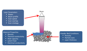
Figure 1: A schematic of the additive manufacturing process using laser powder-bed fusion illustrating the different variables that influence the properties of the part that is produced.

In previous work on additive manufacturing, we considered the problem of determining process parameters for building dense parts. We proposed an iterative approach [13, 12] that combined physics-based computer simulations with simple experiments to generate data that informed the choice of parameters likely to result in high-density parts. Intuitively, we wanted to find parameters that fully melted each layer of powder into the substrate below. Too little energy would result in un-melted powder, which would lead to lower density due to the voids between the powder particles. Too much energy would be wasteful, or worse, could result in keyhole-mode melting [15], with very deep melt pools and the formation of pores that would reduce the density.

In our approach, we started with a very simple, but approximate, physics model to identify the range of viable parameters that resulted in moderate-depth melt pools. We then identified parameters in this range for single-track experiments where we used specific laser power and speed values to melt a fixed thickness of powder spread on a plate. The plate was cut perpendicular to each track to determine how far into the substrate (the plate, in this case) the material had melted. Using these results, we could propose possible power-speed pairs for use in building a dense part.

Our initial physics model, though fast enough to allow us to explore the design space fully, was very simple and therefore, very approximate. As the single track experiments are expensive, we had to carefully select the power-speed combinations so we could gain maximum insight into the process from a limited number of tracks. To enable this selection, we proposed an intermediate step that used a more complex, and accurate, physics model that was run at a small number of points identified by the simpler model. We could then use the resulting data to build a code surrogate that allowed us to predict the output at any point in the input parameter space.

These code surrogates [12, 14] are essentially machine learning models that relate the inputs (the parameters used in AM) to the outputs (the characteristics, such as depth, of the melt-pool). We can use them to solve “inverse problems”, where we identify input parameters that give melt-pool depths in a given range for use in single-track experiments or in improved control of the process through process maps [4] that identify process parameters that result in a fixed value of the melt-pool depths. This map would allow us to maintain constant processing of the powder, for example, when the laser slows down to make a turn.

In our work on using code surrogates to solve inverse problems, we encountered two data-related challenges:

• The computational cost of building a good surrogate: Our prior work [14] showed that two methods — locally weighted kernel regression [2] and Gaussian process (GP) [22] — provide accurate predictions when the data sets are small, which is the case when both experiments and simulations are expensive. GPs are preferable as they provide both the prediction and the uncertainty on the prediction. However, as we perform more experiments and simulations, the size of the data increases, and GP can become too expensive to use, even for moderate sized problems.

• Understanding the solution of the inverse problem: When the number of input parameters is greater than two, it can be challenging to understand where the solution to the inverse problem lies in the input space. The ability to explore the solution in input space is required to gain scientific insight and to understand which input parameters to vary and how to vary them to get the desired output.

We discuss ways to address these challenges in the context of additive manufacturing but observe that they are common to the solution of inverse problems in any application domain.

Our contributions in this paper are as follows: first, inspired by the concept of tapering that introduces sparsity in the covariance matrix to reduce the computational cost, we propose a simple modification, which we call the independent-block GP, and provide guidelines for selecting the blocks such that we improve the speed of GP without sacrificing accuracy. Second, we investigate ways in which we can gain insight into the high-dimensional solutions to inverse problems using parallel coordinate plots and Kohonen self-organizing maps. We show that using weighted distances can lead to a better organized map, providing greater insight.

3 Description of the data

We conduct our investigations using data from the Eagar-Tsai model [7], which is the simple model we used to identify parameters for the single track experiments and sample points for the more complex model. This model considers a Gaussian laser beam moving on a flat plate. The resulting temperature distribution on a three-dimensional spatial grid representing the plate is used to compute the melt-pool depth as a function of four input parameters: laser power, laser speed, laser beam size, and laser absorptivity of the powder, which indicates how much of the laser energy is absorbed by the powder. We generate sample points with stratified random sampling — using the parameter ranges and the number of levels per input specified in Table 1, we place a sample point randomly in each cell, resulting in a 462-sample data set, which we refer to as ET462 [13]. This data set is used in our work on reducing the computational cost of the GP surrogate - it is small enough to permit investigations into different ideas, yet large enough to help us to understand why we need to speed up the surrogate.

Parameter	Minimum	Maximum	Levels
Power (W)	50	400	7
Speed (mm/s)	50	2250	10
Beam size ($\mu$m)	50	68	3
Absorptivity $\eta$	0.3	0.5	2

Table 1: Ranges and number of levels for the stratified random sampling in the four-dimensional input parameter space of the Eagar-Tsai model.

The second data set we use is derived from the ET462 data set and was generated to understand how to display the solution to the inverse problem. We first build a GP model using the ET462 data set and use it to predict output values at 5000 samples in the space defined by the domain in Table 1. We use the best-candidate sampling method [20, 12] to place samples randomly as far apart from each other as possible and use the GP model to generate the melt-pool depth at these points. This data set is referred to as the ET5000 data set. Then, to solve the inverse problem of finding input parameters that result in $60$$\mu$m  depth, we simply identify the sample points with depth values in the range $60\pm\Delta$$\mu$m, where the small interval is used to account for the fact that few inputs give a depth of exactly $60$$\mu$m. We considered two values of $\Delta=2\ \text{and}\ 5$, consisting of 271 and 700 samples, respectively.

4 Speeding up the Gaussian process surrogate

The Gaussian process model (GP) [22], though relatively expensive, is often a good choice as a surrogate model as it provides accurate predictions, as well as an uncertainty on the prediction. We describe GP [8] using a $d$-dimensional problem with a training set of $N$ samples, $\{{\bf x}_{1},\ldots,{\bf x}_{N}\}$ and the associated scalar output values ${\bf y}=\{y_{1},\ldots,y_{N}\}$. Each ${\bf x}_{i}$ is of dimension $d$. The pair $({\bf x}_{i},y_{i})$ is referred to as an instance in the data set. Two samples ${\bf x}_{i}$ and ${\bf x}_{j}$ in the training data are related to each other through the covariance function $k(D)$ where $D$ is the distance between ${\bf x}_{i}$ and ${\bf x}_{j}$. We use the squared-exponential function:

$$k({\bf x}_{i},{\bf x}_{j})=k(D)=\sigma_{f}^{2}\exp\bigg{(}\frac{-D^{2}}{2l^{2}}\bigg{)}+\delta_{ij}\sigma_{n}^{2}$$ (1)

where $\sigma_{f}^{2}$ is the maximum allowable covariance and $l$ is a length parameter that determines the extent of influence of each sample point and thus controls the smoothness of the interpolation. The term $\sigma_{n}^{2}$ accounts for possible noise in the data, with $\delta_{ij}=1$ when $i=j$ and 0 otherwise. We use a weighted Euclidean distance $D$, with weights $w_{m}$ in dimension $m$, defined as

$$D({\bf x}_{i},{\bf x}_{j})=\sqrt{\sum_{m=1}^{d}w_{m}({x}_{im}-{x}_{jm})^{2}}.$$ (2)

as we have found that it gives more accurate predictions by weighting each input dimension based on its importance in predicting the output. These weights, combined with the length parameter, are included in the hyperparameters for GP and determined as described later in this section.

Suppose we want to use the training data to predict the output at a new sample point ${\bf x}_{\ast}$. As the data can be represented as a sample from a multivariate Gaussian distribution, we have

$$\begin{bmatrix}{\bf y}\\ y_{\ast}\end{bmatrix}=\mathcal{N}\Bigg{(}{\bf 0},\begin{bmatrix}{\bf C}&{\bf c}_{\ast}^{T}\\ {\bf c}_{\ast}&c_{\ast\ast}\end{bmatrix}\Bigg{)}\ ,$$

where $\bf y$ is the output variable corresponding to the $N$ training instances, $y_{\ast}$ is the prediction of the output at point ${\bf x}_{\ast}$, and the sub-matrices are defined as follows:

$${\bf C}=\begin{bmatrix}k({\bf x}_{1},{\bf x}_{1})&k({\bf x}_{1},{\bf x}_{2})&\ldots&k({\bf x}_{1},{\bf x}_{N})\\ k({\bf x}_{2},{\bf x}_{1})&k({\bf x}_{2},{\bf x}_{2})&\ldots&k({\bf x}_{2},{\bf x}_{N})\\ \vdots&\vdots&\vdots&\vdots\\ k({\bf x}_{N},{\bf x}_{1})&k({\bf x}_{N},{\bf x}_{2})&\ldots&k({\bf x}_{N},{\bf x}_{N})\\ \end{bmatrix}\ ,$$ (3)

$${\bf c}_{\ast}^{T}=\begin{bmatrix}k({\bf x}_{\ast},{\bf x}_{1})&k({\bf x}_{\ast},{\bf x}_{2})&\ldots&k({\bf x}_{\ast},{\bf x}_{N})\\ \end{bmatrix}\ ,$$

and

$$c_{\ast\ast}=k({\bf x}_{\ast},{\bf x}_{\ast}).$$

The probability of $y_{\ast}$, that is, the output at the new sample point, is then given by

$$\overline{y}_{\ast}={\bf c}_{\ast}^{T}{\bf C}^{-1}{\bf y}$$ (4)

and the uncertainty in the estimate is given by the variance

$$\text{var}(y_{\ast})=c_{\ast\ast}-{\bf c}_{\ast}^{T}{\bf C}^{-1}{\bf c}_{\ast}.$$ (5)

The most expensive step in these equations is solving a system of the form ${\bf C}{\bf u}={\bf v}$. If we are interested only in predictions at new sample points, this system has to be solved only once for all new sample points with ${\bf v}={\bf y}$. But if we are also interested in the variance in the prediction, then the system has to be solved for each new sample point as, from Equation 5, the right-hand side ${\bf v}$ is ${\bf c}_{\ast}$, which depends on the new sample point.

Equations 1 and 2, indicate that the GP model is described by $d+2$ hyperparameters: $\sigma_{f}$, $\sigma_{n}$, and the $d$ weighted length scales $l/w_{i}$ that are used in the distance calculation. To obtain the optimal values for these $d+2$ hyperparameters for our training data set, we use a random search [3] through the $(d+2)$-dimensional space of parameters. To evaluate the quality of each set of hyperparameters, we use the mean absolute error (MAE) for a leave-one-out evaluation, that is, for each sample, we build the GP model using the remaining $(N-1)$ samples, calculate the prediction on the sample held out, and use the mean of the absolute error in prediction across all samples as the quality metric. If $R$ sets of hyperparameters are used to find the optimum, this results in building $R*N$ GP models. This can be a large number when $N$, the number of instances in the data set, is large. Even for moderate $N$, when the dimension $d$ of the problem is large, exploring the high-dimensional hyperparameter space to find the optimal set would require a large value for $R$.

Therefore, to reduce the cost of hyperparameter optimization in building a surrogate model, we can use one or more of the following ideas:

• reduce the number $R$ of sets of hyperparameters considered in the optimization, which could result in identifying a less than optimal set, or

• partially evaluate each set of hyperparameters if possible, and fully evaluate only those found to be promising [19], or

• use a metric that considers only some of the instances in the data set [22], which could result in a less than optimal set of hyperparameters depending on which training instances were used in the evaluations, or

• use an approximate instead of an exact method to solve the linear system in Equations 4 and 5.

In this paper, we focus on the last of these ideas, where we reduce the cost of hyperparameter optimization, not by a less-than-thorough search of the parameter space, but by reducing the cost of evaluating each parameter set through an approximate solution of the linear system. We consider two options: first, the use of a direct solver with an approximate covariance matrix obtained using a simple idea derived from the concept of tapering, and second, an iterative solver, where we control the approximation using the number of iterations.

4.1 Using approximations in a direct solver

To solve the system ${\bf C}{\bf u}={\bf v}$, with the covariance matrix ${\bf C}$ defined in Equation 3, using a direct solver, we first obtain the Cholesky factorization of ${\bf C}={\bf L}{\bf L}^{T}$ and then solve for ${\bf u}$ using two triangular solves ${\bf u}={\bf L}^{-T}({\bf L}^{-1}{\bf v})$. One way to approximate the covariance matrix is by tapering, where we introduce sparsity into the matrix and exploit the sparsity to reduce the computational cost. While we could explicitly set values in the covariance matrix less than a certain threshold, $\theta$, to zero, the resulting matrix could become non-positive-definite [10]. Instead, tapering is applied by multiplying the covariance function by another function $k_{\theta}$

$$k_{taper}(D)=k(D)*k_{\theta}(D)$$ (6)

where $k_{\theta}(D)$ is defined to be 0 if $D\geq\theta$ and a value between 0 and 1 if $D<\theta$. This introduces sparsity while retaining the positive-definiteness of the matrix. Several taper functions have been suggested, for example, the Wendland-1 taper [10]:

$$k_{\theta}(D)=\bigg{(}1-\frac{D}{\theta}\bigg{)}_{+}^{4}\bigg{(}1-4\frac{D}{\theta}\bigg{)}$$ (7)

where $(x)_{+}=max(0,x)$. Figure 2 shows the effect of the Wendland-1 taper on a squared-exponential covariance function based on the distance from a point.

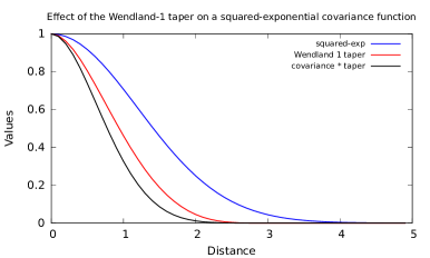
Figure 2: The effect of a Wendland-1 taper, with $\theta=3.0$ applied to a squared-exponential covariance function (Equation 1) with $\sigma_{f}=1.0$, $\sigma_{n}=0.0$ and $l=1.2$. Note that tapering reduces all values of the covariance function.

In our previous work [9], we found that tapering benefited only problems with a specific characteristic. When we introduce sparsity into the covariance matrix, the amount of sparsity must be such that it can be exploited to reduce the computational cost. At the same time, the values being dropped must be very small so that the solution with the tapered covariance matrix is close to that of the original covariance matrix. Both these conditions are satisfied when the function being approximated varies relatively rapidly so that the influence of each sample point is small, i.e., the optimal length scale $l$ in the covariance function is small.

This finding led to two observations. First, tapering would be inappropriate if the function we want to model using GP varies smoothly, not rapidly. This is the case with our additive manufacturing data set, and as the true range of the covariance function is much larger than the tapering range, we cannot introduce sparsity without introducing a large error in the tapered covariance matrix [5]. Second, in the search for optimal hyperparameters we cannot artificially restrict the length scale to be small, as we do not know apriori the true length scale of our data set. So, even if our data set could benefit from tapering, there will be some parameter sets in the hyperparameter optimization that will not benefit from tapering, and the computational costs may not reduce to the extent desired to make the use of GP tractable.

In the course of understanding the conditions under which we could use tapering, we came across a very simple idea in the literature on covariance tapers that had been found to work better than traditional tapers. In a paper discussing the theory behind the choice of a taper [24], Stein found that “for purposes of parameter estimation, covariance tapering often does not work as well as the simple alternative of breaking the observations into blocks and ignoring dependence across blocks.”. As he observes, this idea can be considered as a specific form of a taper, with

$$k_{\theta}({\bf x}_{i},{\bf x}_{j})=\begin{cases}1,&\text{if}\ {\bf x}_{i}\ \text{and}\ {\bf x}_{j}\ \text{are in same block}\\ 0,&\text{otherwise.}\end{cases}$$

A later paper by Bolin and Wallin on adaptive tapers for data sampled at irregular locations [6] also observed that while adaptive tapers outperform regular tapers, block tapering was often a better method for parameter estimation. Unfortunately, neither paper discussed how the data were to be partitioned into blocks; specifically, the dimensions along which we should block the data or the block sizes to use. To partition the observations into blocks such that nearby observations are in the same block, we have two options:

• Block tapering: This is the approach in [24, 6] where the covariance matrix is created as a block diagonal matrix, with each diagonal block corresponding to a block of the data. Though the Cholesky decomposition of each diagonal block is calculated separately, the mean absolute error across all blocks is considered in evaluating a set of hyperparameter values. As a result, a single set of optimal hyperparameters is identified for the data set, though this set may be suboptimal for each block considered independently.

• Independent-block GP: Instead of blocking the covariance matrix, we propose a simple alternative where we apply the blocking at the level of the GP. We split the data set into several smaller non-overlapping blocks along one or more input dimensions and build a separate GP model for each block, which would now have its own set of optimal hyperparameters. To predict the value at a new point, we would find which block it belonged to and use the model for that block. This approach has several benefits: it is easier to implement as the software requires minimal changes, and it can give more accurate results as the hyperparameters selected are optimal for each block as they can now be different across blocks. Further, it allows the possibility of overlapping blocks to build the GP model, which can help in reducing the prediction error at the interior block boundaries. We refer to this algorithm as the independent-block GP method and show how we can exploit the characteristics of the data to select the blocks.

4.2 Using an iterative solver

An alternate way of introducing approximation in the linear solver in an attempt to reduce its computational cost is to use an iterative solver as we can stop the iterations before an accurate solution has been found. Since the covariance matrix (Equation 3) is symmetric positive definite, an obvious choice is the conjugate gradient method [23], described in Algorithm 1.

Algorithm 1 The Conjugate Gradient algorithm to solve ${\bf C}{\bf u}={\bf v}$

1:  Set the threshold $\epsilon$ for the two norm of the residual and $max_{iter}$, the maximum number of iterations.

2:  Set the initial guess for the solution, ${\bf u}_{0}$.

3:  Set initial residual ${\bf r}_{0}={\bf v}-{\bf C}{\bf u}_{0}$ and initial direction vector ${\bf p}_{0}={\bf r}_{0}$.

4:  for $k=0$ to $iter_{max}$ do

5:     Calculate $\alpha_{k}=\frac{{\bf r}_{k}^{T}{\bf r}_{k}}{{\bf p}_{k}^{T}{\bf C}{\bf p}_{k}}$

6:     Update solution vector: ${\bf u}_{k+1}={\bf u}_{k}+\alpha_{k}{\bf p}_{k}$

7:     Update residual vector: ${\bf r}_{k+1}={\bf r}_{k}-\alpha_{k}{\bf C}{\bf p}_{k}$

8:     Calculate $\beta_{k}=\frac{{\bf r}_{k+1}^{T}{\bf r}_{k+1}}{{\bf r}_{k}^{T}{\bf r}_{k}}$

9:     If $\sqrt{{\bf r}_{k+1}^{T}{\bf r}_{k+1}}<\epsilon$ or $(k+1)>max_{iter}$, exit.

10:     Update direction vector: ${\bf p}_{k+1}={\bf r}_{k+1}+\beta_{k}{\bf p}_{k}$

11:  end for

Though the conjugate gradient method is guaranteed to converge in $N$ iterations for a matrix of size $N$, this is rarely the case due to round-off error, especially if the condition number of the matrix is large. Running the algorithm for $N$ iterations would also make it as expensive as a direct solver as each iteration involves a matrix-vector multiply, which is an $\mathcal{O}(N^{2})$ operation. So, we investigated how the solution accuracy was affected when we stopped the iterations i) when the two-norm of the residual became smaller than a threshold, and ii) after a fixed number of iterations smaller than $N$.

5 Understanding the solution of an inverse problem

Once we have built a surrogate model for the forward problem in the form of a Gaussian process, we can use the model to predict the values of the outputs at a relatively dense set of sample points in the input space. The solution to the inverse problem would then be the sample points that meet the target range, as described in Section 3. When the input space is high-dimensional (greater than 2), it is a challenge to understand and interpret the solution points in this space as they cannot be visualized easily. For example, Figure 3 shows the locations of the samples from the ET5000 data set with depth in the range [58,62]$\mu$m  using two input dimensions. For problems with a moderate to large number of input dimensions, such an approach can soon become impractical.

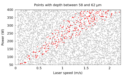
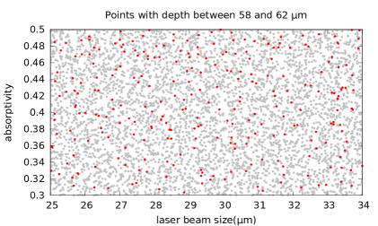
Figure 3: The sample points in the ET-5000 data set that have melt-pool depths in the range [58,62]$\mu$m, shown in red. Left: in the laser power - laser speed space and right: in the beam size - absorptivity space, indicating a pattern in the former, but not in the latter.

In this paper, we consider two methods for the display of high-dimensional data - parallel coordinate plots [11] and Kohonen self-organizing maps [17], which we describe next.

5.1 Parallel coordinate plots

Parallel coordinate plots, or parallel plots, are a visual technique useful for displaying high-dimensional data [11]. Unlike a traditional Cartesian coordinate plot, where we plot two or three dimensions using axes that are orthogonal to each other, in a parallel plot, the axes for all dimensions are placed parallel to each other and perpendicular to a horizontal line. This allows us to visualize more than three dimensions at a time in one plot.

To create a parallel plot for a data set, we first scale the values in each dimension to lie between 0 and 1, or any other minimum and maximum value. Then, an instance in the data set, which would be a point in a $d$-dimensional space, will be represented by a poly line, that is, a sequence of line segments connecting the scaled values of each dimension for that instance on each of the parallel axes.

In our earlier work [13], we used a parallel plot for the ET462 data set to gain insight into the data. We found that laser speed and power were important variables as they were correlated with the depth of the melt pool. As one would intuitively expect, higher laser power and lower laser speed resulted in deep melt pools, while lower laser power and higher laser speed resulted in shallow melt pools. This allowed us to easily identify input parameters for the moderate-sized melt pools of interest. The other two inputs did not appear to be correlated to the depth.

5.2 Kohonen self-organizing maps

A self-organizing map (SOM) [17] is a form of unsupervised neural network that is used to visualize and understand a high-dimensional data set by mapping it into a two-dimensional array using a non-linear projection. While extensive research in SOMs has been conducted over the years, in this paper, we consider a simple, parameter-free, fast version called the Batch Map algorithm [16]. Our choice is motivated by our previous work [21], where we investigated the effects of various parameters in the more complex variants of SOMs and found that the simpler versions worked just as well as the more complex ones, but required fewer parameters.

A two-dimensional SOM model is associated with a grid or lattice of nodes in two dimensions. The grid is defined by an architecture which includes the number of nodes, $NX$ and $NY$ in the $x$ and $y$ direction, respectively, and a grid layout, square or hexagonal, which defines the relative locations of the nodes on the grid. For example, Figure 4 shows the layout of a $10\times 10$ SOM on a hexagonal grid, so named as each interior node has six neighboring nodes that are equidistant from it. We use only hexagonal grids in our work as they have a more uniform neighborhood structure than square grids. Associated with each of the $NX\times NY$ grid nodes are two vectors: a two-dimensional coordinate vector with the ($x$,$y$) coordinates of the node in the grid and a $d$-dimensional weight vector, sometimes called a model vector, where the $d$ dimensions correspond to the features in the input data set.

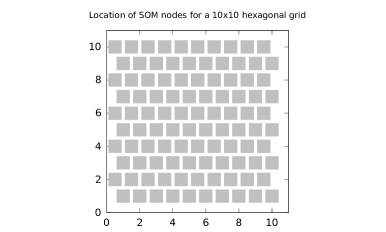
Figure 4: The locations of grid nodes for a $10\times 10$ hexagonal grid. Each node has six immediate neighbors that are equidistant from it, unlike a square grid, where a node has four neighbors at a unit distance and four neighbors $\sqrt{2}$ away.

The SOM algorithm starts by initializing the weight vector at each node of the grid. There are many ways in which this can be done; in our work, we initialize each dimension of the weight vector at a node randomly with a value between the minimum and maximum of the corresponding feature in the data set. Then, the weight vectors are updated using the data set so that they become spatially, globally ordered. As we iterate many times through the instances in the data set, the weight vectors of nodes that are closer to each other in the grid become similar, while the weight vectors of nodes that are far from from each other become less similar [18].

In the online version of the SOM algorithm, the weight vectors are updated by considering an instance at a time, as follows: starting with a random instance, ${\bf x}_{j}$, in the data set, we first find the node $c$, whose weight vector ${\bf m}_{c}$ is the closest to the instance:

$$c=\underset{i\in{1,\ldots,NX\times NY}}{\arg\min}\|{\bf x}_{j}-{\bf m}_{i}\|$$ (8)

where the distance is calculated in the feature space. The node $c$ is called the reference node for the instance ${\bf x}_{j}$. The weight ${\bf m}_{c}$ is then updated to be closer to the instance ${\bf x}_{j}$. In addition, the weights in the nodes in a neighborhood around node $c$ are also updated to be closer to ${\bf x}_{j}$. The neighborhood is defined using the coordinate vectors at the nodes and reduces in size as the iterations progress. The process is repeated with another randomly-selected instance, until we have processed $N$ instances, completing one iteration. As the instances are selected randomly, we may process some instances more than once and others none at all during an iteration. The iterations repeat until the node weights stabilize.

A faster and simpler version of the SOM algorithm is the batch version which finds the closest reference nodes to all instances first. It then updates the weight vector in each reference node with the nearest instances. This is followed by updates to the nodes in the neighborhood of the reference node of each instance. Typically, the weights in the neighborhood nodes are updated based on how far these nodes are from the reference node, with farther away nodes being updated by a smaller amount. In the Batch Map algorithm [16], which is described in Algorithm 2, this condition is simplified even further and all nodes in the neighborhood are updated to the same extent regardless of their distance to the reference node.

Both the online and batch versions of the self-organizing map operate on the features of the instances and organize the instances in this input feature space, without taking into account the output associated with each instance. The batch version can be considered as deterministic compared to the stochastic online version. Both algorithms start with a random assignment of initial weight vectors. But, as there is no randomness in the processing of the instances in the batch algorithm, the weight vectors stabilize and, unlike the online version, give the same results when the algorithm is run repeatedly.

Algorithm 2 The Batch Map algorithm

1:  Set $NX$ and $NY$, the number of grid nodes in the $x$ and $y$ direction, respectively.

2:  Generate the grid coordinates for each node.

3:  Set $r_{max}$ and $r_{min}$, the initial and final radii of the neighborhood, and $r_{iter}$, the number of iterations over which the radius is decreased from $r_{max}$ to $r_{min}$.

4:  Set the current neighborhood radius to $r_{max}$ and define $r_{delta}=(r_{max}-r_{min}/r_{iter})$.

5:  Set $iter_{max}$, the maximum number of iterations.

6:  Initialize the weight vectors at each node.

7:  for $i=1$ to $iter_{max}$ do

8:     for $inode=1$ to $NX\times NY$ do

9:        List the instances nearest to the weight vector of $inode$ or nodes in its neighborhood.

10:     end for

11:     for $inode=1$ to $NX\times NY$ do

12:        Replace the weight vector at $inode$ by the mean of the instances in its list.

13:     end for

14:     Exit if SOM has converged.

15:     Reduce the radius of the neighborhood by $r_{delta}$, without going below $r_{min}$.

16:  end for

The Batch Map algorithm is summarized in Algorithm 2. This algorithm has six parameters: $NX$ and $NY$, the number of grid nodes in the $x$ and $y$ dimension, respectively; $r_{max}$ and $r_{min}$, the initial and final radii of the neighborhood, respectively; $r_{iter}$, the number of iterations over which the radius is decreased from $r_{max}$ to $r_{min}$; and $iter_{max}$, the maximum number of iterations of the SOM algorithm, where one iteration involves a pass through all instances in the data set. Instead of stopping after a fixed number of iterations, we can also monitor a convergence metric such as

$$\frac{1}{N}\sum_{i=1}^{N}\|{\bf x}_{i}-{\bf m}_{c}\|$$ (9)

which is the average distance of each instance to the nearest node. A SOM has stabilized when this metric does not change over iterations or the maximum number of iterations has been reached. Since the Batch Map is fast enough for our data sets, we just let it run for $iter_{max}$ iterations, which is chosen to be suitably large so that the metric above stabilizes.

For our work with SOMs, we use two grids, one of size $30\times 30$ and the other of $10\times 10$. For the larger grid, we use $r_{max}=20$, $r_{min}=1$, $r_{iter}=150$ and $iter_{max}=200$. The corresponding values for the smaller grid are 8, 1, 100, and 120. $r_{max}$ was set as a large fraction of the grid size $NX$, while $r_{iter}$ was set by experimentation to be large enough to allow the map to self organize. We found that the ierations stabilized soon after $r_{iter}$, which led to the choice of $iter_{max}$. Batch Map is a very fast algorithm, and as it required no more than a few seconds for our data sets, we were able to experiment with various parameter values. We also found that the results were remarkably robust to the parameter settings.

6 Experimental results and discussion

We next present the results of our experiments with approximate solvers for GP using the ET462 data set and high-dimensional data exploration methods with the ET5000 data set.

All times reported in this paper are for codes run on an Intel Xeon W-2155 workstation with ten cores, two threads per code, and 62GB of memory. The codes are run on a single core.

6.1 Evaluating independent-block GP

In independent-block GP, we divide the input domain into blocks of sample points and ignore the dependence between the blocks. To accomplish this, we need to determine:

• The number of blocks to use: Suppose we divide the data into $B$ blocks. Then, with $N$ data points in the data set, each block will have $(N/B)$ data points if $N$ is divisible by $B$; if not, we can divide the data so the blocks have roughly equal number of points. Solving a linear system with $N$ equations using a direct method requires $\mathcal{O}(N^{3})$ floating point operations. For $B$ blocks, this reduces to $B*\mathcal{O}((N/B)^{3})$, a $B^{2}$ reduction in the computations. This makes blocking a very appealing idea if it does not result in lower predictive accuracy. To maintain the accuracy, we need to ensure that each block has a sufficient number of data points, which limits how many blocks we can create. In our work we use $B=2\ \text{and}\ 4$.

• The dimension(s) along which to block the data: We tried two options - blocking along just one dimension and blocking using two of the four input dimensions. Blocking along additional dimensions, though an option for large datasets, would have resulted in too many blocks and too few samples in each block for our dataset.

To generate results for hyper-parameter optimization using independent-block GP, we considered 100 samples in the six-dimensional GP hyper-parameter space: $\sigma_{f}$, $\sigma_{n}$, and the four weighted length scales $l/w_{i},i=1,\ldots,d$ that are used in the distance calculation. As with the generation of samples for the ET5000 data set, these six-dimensional samples were also generated using the best candidate method [20], which, by placing the samples randomly, but far apart from each other, allowed us to explore the hyperparameter space fully. For a fair comparison, we used the same 100 hyperparameter samples across all our experiments. We compared the quality of the prediction using the predicted vs. actual value for the instances in each block, where the predicted value is obtained using a GP model built with the remaining instances in the block.

For the direct solver, we use the optimized BLAS and LAPACK solvers for the symmetric matrix stored in the packed storage format, while the conjugate gradient method uses the BLAS 2 matrix vector multiply algorithm, with the matrix stored in the symmetric packed storage [1]. All computations are in double precision. We did invesitgate the use of single precision Cholesky solvers, but found that the system had to be very large for a substantial reduction in time. In addition, depending on the hyperparameters, the covariance matrix could become singular in single precision.

In the tables with the results for independent-block GP, we also report the total time for hyperparameter optimization to find the best of 100 samples for a data set with $M$ instances, where $M$ is the size of a block. For each hyperparameter sample, we perform a leave-one-out (LOO) analysis that involves the creation and solution of $M$ systems of equations, each of size $(M-1)$. In addition, we perform two leave-one-out analyses, one with a default set of hyperparameters and the other with the optimal set. For these two cases, we also generate the variance on the prediction of the instance held out from the data.

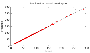
$\sigma_{f}$	$\sigma_{n}$	$l/w_{1}$	$l/w_{2}$	$l/w_{3}$	$l/w_{4}$	MAE (opt)
4.015e-05	2.080e-07	0.157	0.327	1.451	1.735	5.27e-07

Figure 5: Predicted vs. actual values of the melt pool depth for the full ET462 data set (no blocking), obtained using the LOO method and the optimal hyperparameters listed in the table. MAE is the mean absolute error at the optimal parameters. Determining the optimal hyperparameters for the original data took 1979s.

First, in Figure 5, we show the LOO accuracy of GP on the full ET462 data set with the optimal hyperparameters used to generate these results. For independent-block GP, we created the blocks by splitting the points in an input dimension based on their values; this may result in slightly unequal blocks if there is more than one point with the same input value. We then ran the GP on each individual block and found the optimal set of hyperparameters from the 100 samples. Figures 6, 7, and 8 present the results with two blocks along each input dimension, four blocks along each input dimension, and four blocks split $2\times 2$ across two input dimensions, respectively. In each figure, we first show the values of the melt-pool depth variable as a function of the input variable used in the split, followed by the performance of GP on each block using the optimal parameters identified for that block. The corresponding optimal hyperparameters for each block for the different blocking schemes are in Tables 2, 3, and 4. The tables also include the time for processing each block, the speedup relative to processing the full data set, and the mean absolute error in prediction for each block at the optimal values of the hyperparameters.

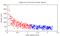
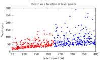
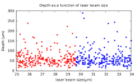
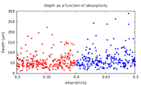
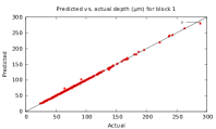
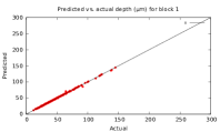
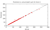
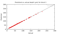
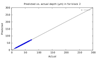
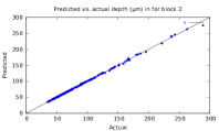
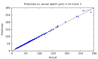
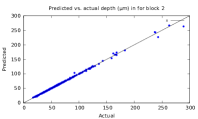
Figure 6: GP predictions with two blocks along each dimension. From left to right: blocking on the laser speed, laser power, laser beam size, and absorptivity. Top row: values of melt-pool depth as a function of the values of each input; red is low values and blue is high values. The predicted vs. actual values for the depth for points with lower values of the input (in red, middle row) and higher values of the input (in blue, bottom row).

Block	Block	Time	$\sigma_{f}$	$\sigma_{n}$	$l/w_{1}$	$l/w_{2}$	$l/w_{3}$	$l/w_{4}$	MAE
variable	number	(s)							(opt)
Speed	1000	226	3.855e-05	2.348e-07	0.185	1.107	1.781	1.973	7.08e-07
	2000	226	2.385e-05	4.143e-07	1.271	0.393	1.568	1.966	2.89e-07
Power	0100	223	3.855e-05	2.348e-07	0.185	1.107	1.781	1.973	4.72e-07
	0200	229	2.787e-05	2.683e-07	0.142	1.151	1.536	1.293	6.79e-07
Beam size	0010	231	2.101e-05	2.061e-07	0.102	0.668	1.891	1.445	7.73e-07
	0020	220	3.333e-05	2.450e-07	0.133	0.750	1.460	1.708	9.14e-07
Absorptivity	0001	226	3.855e-05	2.348e-07	0.185	1.107	1.781	1.973	7.26e-07
	0002	226	3.333e-05	2.450e-07	0.133	0.750	1.460	1.708	9.79e-07

Table 2: Optimum hyperparameters, with mean absolute error (MAE), for blocking along one dimension with two blocks. The block number has four digits in order of input variables. A value of 1 indicates lower values and 2 indicates higher values of the input; 0 indicates no blocking. Thus block 0100 has lower values of the second input parameter, the laser power. Each block has roughly (462/2 = 231) sample points. The speedup compared to no blocking is 4.38 - 4.39.

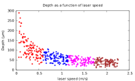
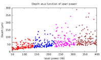
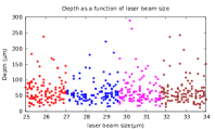
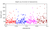
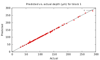
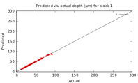
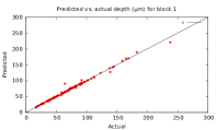
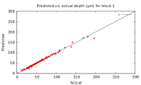
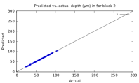
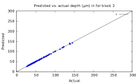
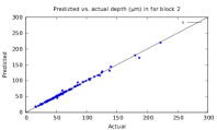
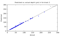
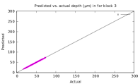
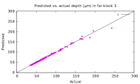
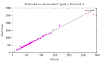
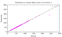
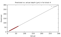
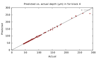
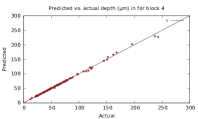
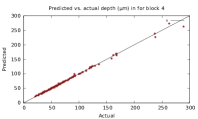
Figure 7: GP predictions with four blocks along each dimension. From left to right: blocking on the laser speed, power, beam size, and absorptivity. Top row: the values of melt-pool depth as a function of each of the inputs. Rows two through five: the LOO predicted vs. actual values for the depth corresponding to points with increasingly larger values of the input (coded by color).

Block	Block	Time	$\sigma_{f}$	$\sigma_{n}$	$l/w_{1}$	$l/w_{2}$	$l/w_{3}$	$l/w_{4}$	MAE
variable	number	(s)							(opt)
Speed	1000	27	5.300e-05	4.295e-07	0.282	0.612	1.248	1.902	9.51e-07
	2000	28	4.771e-05	3.842e-07	1.867	0.789	1.974	1.803	3.46e-07
	3000	29	3.055e-05	4.341e-07	1.860	0.320	1.680	1.847	3.11e-07
	4000	28	5.584e-05	4.068e-07	1.895	0.572	1.281	1.731	3.08e-07
Power	0100	28	3.314e-05	2.908e-07	0.247	1.543	1.941	1.601	5.11e-07
	0200	27	3.855e-05	2.348e-07	0.185	1.107	1.781	1.973	5.54e-07
	0300	29	2.787e-05	2.683e-07	0.142	1.151	1.536	1.293	1.47e-06
	0400	27	2.795e-05	2.292e-07	0.171	1.247	1.115	1.701	1.30e-06
Beam size	0010	27	3.855e-05	2.348e-07	0.185	1.107	1.781	1.973	1.49e-06
	0020	29	3.152e-05	1.571e-07	0.253	1.221	1.449	1.961	1.10e-06
	0030	24	3.855e-05	2.348e-07	0.185	1.107	1.781	1.973	2.23e-06
	0040	30	3.385e-05	3.018e-07	0.156	0.749	1.167	1.969	1.21e-06
Absorptivity	0001	27	3.806e-05	1.277e-07	0.261	0.823	1.888	1.617	1.40e-06
	0002	28	3.855e-05	2.348e-07	0.185	1.107	1.781	1.973	1.37e-06
	0003	26	3.855e-05	2.348e-07	0.185	1.107	1.781	1.973	1.31e-06
	0004	29	3.333e-05	2.450e-07	0.133	0.750	1.460	1.708	1.61e-06

Table 3: Optimum hyperparameters, with mean absolute error (MAE), for blocking along one dimension with four blocks. The block number has four digits in order of input variables. Values of 1,2,3, and 4 indicate low to high input values; 0 indicates no blocking. Each block has roughly (462/4 = 115) sample points. The speedup compared to no blocking is 17.67 - 17.99.

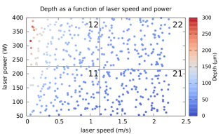
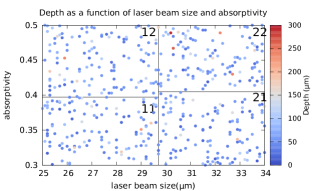
(a)		(b)

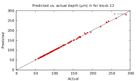
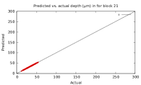
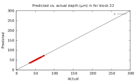
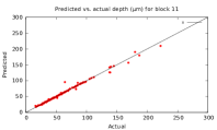
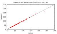
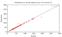
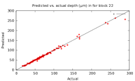
Figure 8: GP predictions with four blocks along two dimensions. (a) blocking in the laser speed and laser power inputs. (b) blocking in the laser beam size and absorptivity inputs. Each block is numbered in its top right corner. Middle and bottom rows correspond to (a) and (b), respectively, and show the LOO predicted vs. actual values for the depth for each block, from left to right: block 11, 12, 21, and 22.

Block	Block	Time	$\sigma_{f}$	$\sigma_{n}$	$l/w_{1}$	$l/w_{2}$	$l/w_{3}$	$l/w_{4}$	MAE
variables	number	(s)							(opt)
Speed	1100	27	3.855e-05	2.348e-07	0.185	1.107	1.781	1.973	6.82e-07
and	1200	28	3.855e-05	2.348e-07	0.185	1.107	1.781	1.973	8.54e-07
power	2100	27	4.209e-05	5.392e-07	1.751	1.044	1.953	1.961	2.90e-07
	2200	28	3.746e-05	5.059e-07	0.864	1.251	1.316	1.966	2.86e-07
Beam size	0011	27	3.855e-05	2.348e-07	0.185	1.107	1.781	1.973	1.88e-06
and	0012	29	3.152e-05	1.571e-07	0.253	1.221	1.449	1.961	1.39e-06
absorptivity	0021	27	3.855e-05	2.348e-07	0.185	1.107	1.781	1.973	1.48e-06
	0022	27	4.361e-05	3.459e-07	0.091	0.292	1.558	1.654	2.47e-06

Table 4: Blocking on two dimensions, four blocks: optimum parameters and mean absolute error (MAE) for each block. The four digits in each block number indicate the order of input variables. Values of 1 indicate lower input values and 2 indicates higher values of the input; 0 indicates no blocking on that input. Each block has roughly (462/4 = 115) sample points. The speedup compared to no blocking is 17.99.

We next make several observations on these plots and tables:

• Accuracy of predictions with independent-block GP: Overall, we find that the accuracy of the predictions of melt-pool depth with blocking is very good, regardless of the number of blocks or the dimensions along which the blocks are created. As we move from two blocks to four blocks, we see increased scatter around the $y=x$ line that denotes exact prediction. This behavior is also confirmed by the values of mean absolute error in the tables. A careful study indicated that there is pattern to this increased error. We know that the depth values are large at very low values of speed and high values of power. If many, or all, of these large depth instances are in one block, the prediction accuracy is good, which is the case, for example, when we split the speed dimension into four blocks. But, if the blocking distributes the instances with large depth across the blocks, there are too few such instances in each block and the prediction accuracy suffers. This suggests that we should block along the dimension(s) that allow us to keep instances with similar output values within a block.

• Optimal hyperparameter values for each block: In light of the preceding obervation, we would expect that the hyperparameters for the different blocks would likely be different from that of the full data set. The hyperparameter, $l/w_{i}$, indicates the importance of the $i$-th dimension, with a smaller value indicating greater importance. We also know from our previous work [13, 12] that for the melt-pool depth for the full data set, the laser speed is a more important input than laser power, and both beam size and absorptivity are less important. This is confirmed by the hyperparameters in Figure 5. But, when we block on the laser speed input, its importance reduces for blocks with little variation in the speed, as seen in the second row of Table 2 and the second through fourth rows in Table 3. This would suggest that implementing blocking by dividing the data into separate GP models, as we have done, is a better option than creating a single model with a block diagonal covariance matrix, as it allows the hyperparameters to adapt to the characteristics of the data in each block, resulting in more accurate predictions.

• Reduction in compute time: We expect that blocking would reduce compute time for hyperparameter optimization by a factor of $B^{2}$. In fact, the speedup values in the captions of the tables show that we obtain a better than $B^{2}$ speedup; this is the result of improved cache performance as blocking also reduces the size of the covariance matrices, leading to less communication within the memory system. Thus, for even for small values of $B$, such as 2 and 4, we obtain a speedup of 4.4 and nearly 18, respectively. Further speedup can be obtained by observing that the $B$ blocks can be processed in parallel, without incurring any extra overhead. This would result in a greater than $B^{3}$ speedup overall.

• Number of blocks to create: While it is tempting to increase $B$ to reduce the computational time, this would reduce the size of each block. If the blocking is along one dimension, each block would be “skinny”, covering a small range of values in that dimension, which would give lower accuracy as most instances would be near an internal block boundary. This would suggest blocking along more than one dimension if we want more blocks.

• Number of dimensions along which to block the data: For our data set, the results for blocking along two dimensions were no worse than blocking along a single dimension. However, it is possible that for some data sets, blocking along two, or more, dimensions could result in lower prediction accuracy at instances near the corners of the blocks. This, and similar effects at instances near internal block boundaries, could be resolved by using overlapping blocks for building the models; the output at a new instance would then be predicted using the model for the block to which the instance would be assigned in the absence of overlap.

Overall, we conclude that the reduction in compute time makes independent-block GP a very useful idea, especially if we can choose the blocks to minimize the overall scatter across the output values in the blocks.

6.2 Evaluating iterative solvers

We conducted our experiments with iterative solvers by replacing all calls to the direct solver in our code with a call to the conjugate gradient solver described in Algorithm 1. To obtain an approximate solution for the full data set, we considered two options. First, we set the maximum iterations to 462, which is the size of the system, and experimented with two values — 1.0e-3 and 1.0e-4 — of the threshold on the two norm of the residual. The iterations would stop when either of these two conditions was satisfied. We present the results in Figure 10(a) and (b) for the optimal hyperparameters. In evaluating the results, we found that for some sets of hyperparameter values, the residual did not meet the threshold criterion even after 462 iterations, suggesting that the covariance matrix is ill-conditioned for these hyperparameters.

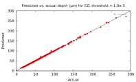
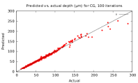
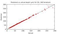
(a)	(b)	(c)	(d)

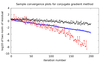
Figure 9: GP predictions using an iterative solver. The results show the LOO predicted vs. actual values of the melt-pool depth obtained using the optimal hyperparameters. (a) residual threshold = 1.0e-4, maximum iterations = 462, time = 3570s. (b) residual threshold = 1.0e-3, maximum iterations = 462, time = 3425s. (c) maximum iterations = 100, time = 1982s. (d) maximum iterations = 200, time = 2496s.

Figure 10: Convergence of the conjugate gradient solver for three different sets of hyperparameters, illustrating fast convergence in some cases, with the two norm of the residual reducing to 1.0e-8 in less than 200 iterations for a system of size 462, but quite slow and noisy in other cases.

Next, for greater control over the iterative process, we set the maximum number of iterations to two values — 100 and 200 — with a very low value of 1.0e-8 for the residual threshold. The results are presented in Figure 10(c) and (d). Our expectation was that for all 100 sets of hyperparameter values, the constraint on the number of iterations would occur before the residual reduced below the threshold. However, we found that this was not always the case, suggesting that some parameter sets resulted in very well-conditioned systems. Figure 10 shows the large disparity among convergence rates for three sample sets of hyperparameters. We also found that stopping the process after 100 iterations frequently meant that the iterations were far from converging, and likely to identify a less-than-optimal set of hyperparameters, resulting in the higher prediction error shown in Figure 10(c).

Overall, a key observation in our experiments with iterative solvers was that they were slow. Even the fastest case, with a limit of 100 iterations, at 1982s, took just as long as the direct solver on the full data set at 1979s (Figure 5), but gave less accurate results, as indicated by the scatter in Figure 10(c). Unlike the direct solvers, it is also challenging to find appropriate stopping criteria for the iterative solvers.

Finally, we observe that it is possible to improve the convergence of the iterative solvers using preconditioning [23]. A possible preconditioner would be a block diagonal preconditioner, but, our experiences in Section 6.1 suggest that the independent-block GP method would be computationally faster.

6.3 Understanding the high-dimensional solution space

We next explored the four-dimensional solution space in which instances from the ET5000 data set with depth in the range $60\pm\Delta$, with $\Delta=2\ \text{and}\ 5$, lie using parallel coordinate plots and Kohonen self organizing maps that were described in Sections 5.1 and 5.2, respectively.

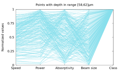
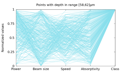
Figure 11: Parallel plots showing the points in the ET-5000 data set with melt-pool depth in the range [58,62]$\mu$m. Two different ordering of the four input variables are shown, which allows each variable to be plot adjacent to each of the remaining three variables. The class value of 1 indicates that these are points that meet the criterion on the melt-pool depth.

First, in Figure 11, we show the solution instances with depth $60\pm 2$ in parallel coordinates. As this data set has only 271 instances, the smaller number of points makes it easier to identify patterns in the solution. We consider two different orderings of the input dimensions to ensure each variable can be adjacent to all remaining variables. We observe that for the solution instances, speed and power have a nearly linear relationship as the lines connecting the two are nearly, but not perfectly, horizontal. The solution has few points at both low and high values of speed (based on the sparsity of points at the extreme ends of the speed axis), and has more instances at higher values of the power axis. This agrees with the plot in the left panel of Figure 3. It is however difficult to draw any additional conclusions regarding the solution to the inverse problem from the parallel plots, though we found them invaluable in understanding the full dataset itself [13].

The self organizing maps provide a very different insight into the solution to the inverse problem. In our work, we considered two options for the distance in Equation 8 to find the reference node - Euclidean distance and weighted Euclidean distance, where we used as weights the inverse of the weighted length scales from Figure 5, as a smaller length scale in GP indicates a more important input.

First, in Figures 12 and 13, we show results for a $30\times 30$ map for the ET5000 data set using unweighted and weighted distances, respectively. The four plots in the top row of each figure show the value of each dimension in the weight vector at the SOM nodes, followed in the second row by some statistics on the instances assigned to each node. As the 5000 instances in the data set are spread out uniformly in the input domain, we do not expect the SOM to identify any topological structure in the location of the instances in the data set.

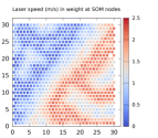
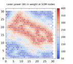
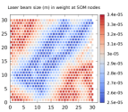
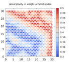
(a)	(b)	(c)	(d)
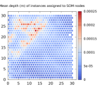
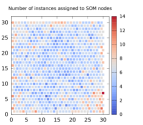
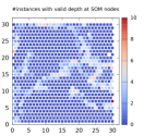
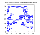
(e)	(f)	(g)	(h)

Figure 12: Results for the ET5000 data set using a $30\times 30$ SOM and unweighted distances. (a)-(d) show the values of the weights at each SOM node in the four input dimensions — speed, power, beam size, and absorptivity. (e) Mean value of the instances assigned to each SOM node. (f) Number of instances assigned to each SOM node. (g) Number of instances with melt-pool depth in range [55,65]$\mu$m  at each SOM node, with the SOM nodes with non-zero such instances hightlighted in (h). Note that there is a node with no instances assigned to it near the right edge.

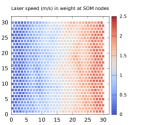
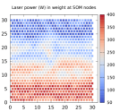
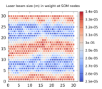
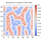
(a)	(b)	(c)	(d)
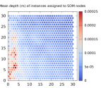
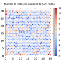
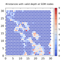
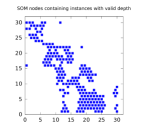
(e)	(f)	(g)	(h)

Figure 13: Results for the ET5000 data set using a $30\times 30$ SOM and weighted distances. (a)-(d) show the values of the weights at each SOM node in the four input dimensions — speed, power, beam size, and absorptivity. (e) Mean value of the instances assigned to each SOM node. (f) Number of instances assigned to each SOM node. (g) Number of instances with melt-pool depth in range [55,65]$\mu$m  at each SOM node, with the SOM nodes with non-zero such instances hightlighted in (h).

We observe that weighted distances result in a better “organized” SOM as the transition from the high to low values of an input variable, such as speed and power, is quite smooth. In contrast, with unweighted distances, the regions with very low-valued points (in dark blue) and the very high valued points (in dark red) both have medium-valued regions (in lighter blue and red) in them. In comparing panels (a) and (b) with panel (e) for both weighted and unweighted distances, we observe that deep melt pools occur at low values of speed and higher values of power, with the correlation being clearer in plots using weighted distances. Figures 12 and 13 also show the number of instances assigned to each SOM node, aas well as the SOM nodes that have instances with depth in the range [55,65]$\mu$m. The latter indicate that the solution to the inverse problem is spread out in the four-dimensional input space in the form of “veins”, rather than clustered in a bunch, in which case they would have appeared in a few nodes that are close to each other.

Next, we construct a $10\times 10$ SOM using just the 700 instances with depth in the range [55,65]$\mu$m; a smaller number of nodes is used as the data set is smaller. Figure 14 shows the mean value of the output at each SOM node; as the range of outputs is quite small, the plots are unremarkable. However, Figure 15 that shows the values of the weight vectors in each dimension using unweighted (top) and weighted (bottom) distances is a lot more interesting. First, as with the full ET5000 data set, we see that using a weighted distance results in a better “organized” SOM as the variation of weights across the nodes, especially in the speed and power dimensions, is much smoother than with unweighted distances. We also note that the solution spans the full range in all four input dimensions, furthur confirming that the solution is not a tight cluster.

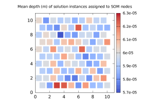
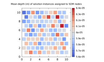
Figure 14: Solution instances, with melt-pool depth in range [55,65]$\mu$m, after processing using a $10\times 10$ SOM. The plots show the mean value of the melt-pool depth for the instances assigned to each node using unweighted (left) and weighted (right) distances.

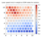
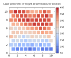
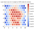
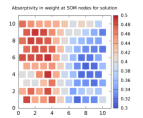
(a)	(b)	(c)	(d)
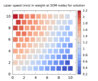
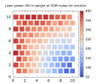
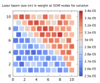
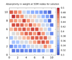
(e)	(f)	(g)	(h)

Figure 15: Solution instances, with melt-pool depth in range [55,65]$\mu$m, after processing using a $10\times 10$ SOM. The plots show the weight at each SOM node for the four inputs from left to right — (a) speed, (b) power, (c) beam size, and (d) absorptivity — using unweighted (top row, a-d) and weighted (bottom, e-h) distances.

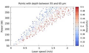
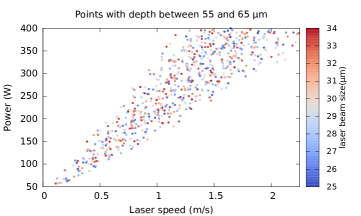
Figure 16: Solution instances, with melt-pool depth in range [55,65]$\mu$m, in the speed and power space, with points colored by absorptivity (left) and laser beam size (right).

We next focus on the results with weighted distances (Figure 15, panels (e)-(h)), to interpret the values in the corresponding nodes of the SOM across the four dimensions and understand where the solution lies in the four-dimensional input space. The plot for speed (panel (e)) has few nodes with very high or very low speed, indicating few such points in the solution, while the plot for power (panel (f)) has more nodes at higher power (in red) than at lower power (in blue). Looking at corresponding nodes in these two plots, we notice that instances at high power (along left and top edges of the SOM in panel (f)) have speed ranges that are medium to high in panel (e). However, instances at low power in the lower right corner of panel (f) have, in the corresponding nodes of panel (e), speed values that are also low. These observations are also corroborated by the plot in the left panel of Figure 3 that indicates that at low power, the solution exists across a narrow range of speed values, but at high power, the solution spans a broader range of speed values. Also, as expected, to keep the melt-pool depth roughly constant, when the power is high (low), the speed is also high (low).

The SOM results in Figure 15, bottom row, also allow us to interpret the values in the corresponding nodes in the other two dimensions. We note that the node values for the beam size vary less smoothly than the values for absorptivity, suggesting that beam size plays a less important role in determining the melt pool depth. The variation in beam size (high at top right reducing to low values at bottom left), is orthogonal to the variation in the power and speed, which is high at top left and low at bottom right. So, at any value of the power or speed, the solution spans nearly the full range of beam sizes. This is especially clear for nodes that have high values of power, along the top and left edges of the SOM.

We also observe that for these nodes with a high value of power, the nodes with a high value of speed (panel (e), top left) coincide with a high value of absorptivity. As the speed reduces from left to right and top to bottom, the absorptivity also reduces. The same behavior also holds at moderate values of power. This suggests that if we create a plot with the solution points in the speed and power space, colored by the absorptivity, then, for a given power value, we should see the absorptivity being high at high speed and low at low speed. This is confirmed by Figure 16, left panel. On hindsight, this finding is not unexpected — for near-constant depth at a given power, if we increase the speed, we should increase absorptivity to keep the energy input near constant. In our problem, we cannot explicitly control the absorptivity of the material; we used a range of values simply to account for the uncertainty in the value. But it is interesting none-the-less that the SOMs were able to identify the importance of absorptivity, especially as it is non-trivial, even with just four inputs, to find such a pattern simply by projecting the solution on subsets of the input dimensions. In Figure 16, right panel, we include a similar plot using beam size, which, as expected, shows that beam size does not play an important role in the solution.

7 Conclusions

In this paper, we considered two issues that make it challenging to solve inverse problems — the slow speed of code surrogates, such as Gaussian processes, and our inability to understand and interpret the solution in a high dimensional input space. We evaluated our proposed solutions to these issues using a problem from additive manufacturing. We showed how the simple idea of independent-block GP can be used to speed up Gaussian processes substantially, without a loss in prediction accuracy. By dividing the data into $B$ blocks, we could obtain a speed up of at least $B^{2}$, or $B^{3}$ if we parallelized the algorithm across the blocks. We also discussed how we should identify the dimensions on which to block the data and the number of blocks to create. To address the second issue, we found that using parallel coordinate plots did not offer much insight into the solution to our inverse problem in the four-dimensional input space. However, Kohonen maps, especially when used with weighted distances, were a simple and robust technique that allowed us to interpret the solution to the inverse problem.

8 Acknowledgment

LLNL-TR-818722 This work performed under the auspices of the U.S. Department of Energy by Lawrence Livermore National Laboratory under Contract DE-AC52-07NA27344. This work is part of the IDEALS project funded by the ASCR Program (late Dr. Lucille Nowell, Program Manager) at the Office of Science, US Department of Energy.

The early work on tapering was performed by Juliette Franzman, undergraduate at UC Berkeley, during a summer internship in 2019. The early work on Kohonen maps was performed by Ravi Ponmalai, undergraduate at UC Irvine, during a summer internship in 2019.

References

- [1] Anderson, E., Bai, Z., Bischof, C., Blackford, S., Dongarra, J. D. J., Croz, J. D., Greenbaum, A., Hammarling, S., McKenney, A., and Sorensen, D. LAPACK Users’ Guide, third ed. SIAM, Philadelphia, Pennsylvania, USA, 1999.
- [2] Atkeson, C., Schaal, S. A., and Moore, A. W. Locally weighted learning. AI Review 11 (1997), 75–133.
- [3] Bergstra, J., and Bengio, Y. Random search for hyper-parameter optimization. Journal of Machine Learning Research 13 (2012), 281–305.
- [4] Beuth, J., et al. Process mapping for qualification across multiple direct metal additive manufacturing processes. In International Solid Freeform Fabrication Symposium, An Additive Manufacturing Conference, D. Bourell (Ed.), University of Texas at Austin, Austin, Texas (2013), pp. 655–665.
- [5] Bolin, D., and Lindgren, F. A comparison between markov approximations and other methods for large spatial data sets. Computational Statistics & Data Analysis 61 (2013), 7 – 21.
- [6] Bolin, D., and Wallin, J. Spatially adaptive covariance tapering. Spatial Statistics 18 (06 2015).
- [7] Eagar, T., and Tsai, N. Temperature-fields produced by traveling distributed heat-sources. Welding Journal 62 (1983), S346–S355.
- [8] Ebden, M. Gaussian process for regression and classification: A quick introduction. Available at http://arxiv.org/abs/1505.02965, submitted May 2015, 2008.
- [9] Franzman, J., and Kamath, C. Understanding the Effects of Tapering on Gaussian Process Regression. Tech. Rep. LLNL-TR-787826, Lawrence Livermore National Laboratory, Livermore, CA, August 2019. Available at https://www.osti.gov/servlets/purl/1558874.
- [10] Furrer, R., Genton, M. G., and Nychka, D. Covariance tapering for interpolation of large spatial datasets. Journal of Computational and Graphical Statistics 15, 3 (2006), 502–523.
- [11] Inselberg, A. Parallel Coordinates: Visual Multidimensional Geometry and Its Applications. Springer, New York, NY, 2009.
- [12] Kamath, C. Data mining and statistical inference in selective laser melting. International Journal of Advanced Manufacturing Technology 86 (September 2016), 1659–1677.
- [13] Kamath, C., El-dasher, B., Gallegos, G. F., King, W. E., and Sisto, A. Density of additively-manufactured, 316L SS parts using laser powder-bed fus ion at powers up to 400 W. International Journal of Advanced Manufacturing Technology 74 (2014), 65–78.
- [14] Kamath, C., and Fan, Y.-J. Regression with small data sets: a case study using code surrogates in additive manufacturing. Knowledge and Information Systems 57 (2018), 475–493.
- [15] King, W. E., et al. Observation of keyhole-mode laser melting in laser powder-bed fusion additive manufacturing. Journal of Materials Processing Technology 214, 12 (2014), 2915 – 2925.
- [16] Kohonen, T. Things you haven’t heard about the self-organizing map. In IEEE International Conference on Neural Networks (1993), vol. 3, pp. 1147–1156 vol.3.
- [17] Kohonen, T. Self-Organizing Maps, 3rd ed. Springer-Verlag, Berlin, Heidelberg, 2000.
- [18] Kohonen, T. Essentials of the self-organizing map. Neural Networks 37 (2013), 52 – 65. Twenty-fifth Anniversay Commemorative Issue.
- [19] Li, L., Jamieson, K., DeSalvo, G., Rostamizadeh, A., and Talwalkar, A. Hyperband: A novel bandit-based approach to hyperparameter optimization. Journal of Machine Learning Research 18, 185 (2018), 1–52.
- [20] Mitchell, D. P. Spectrally optimal sampling for distribution ray tracing. Computer Graphics 25, 4 (1991), 157–164.
- [21] Ponmalai, R., and Kamath, C. Self-Organizing Maps and Their Applications to Data Analysis. Tech. Rep. LLNL-TR-791165, Lawrence Livermore National Laboratory, Livermore, CA, September 2019. Available at https://www.osti.gov/servlets/purl/1566795.
- [22] Rasmussen, C. E., and Williams, C. K. I. Gaussian Processes for Machine Learning. MIT Press, Cambridge, MA, 2006.
- [23] Saad, Y. Iterative Methods for Sparse Linear Systems, 2nd ed. Society for Industrial and Applied Mathematics, USA, 2003.
- [24] Stein, M. L. Statistical properties of covariance tapers. Journal of Computational and Graphical Statistics 22, 4 (2013), 866–885.