Input Rate Control in Stochastic Road Traffic Networks:
Effective Bandwidths

Abstract.

In road traffic networks, large traffic volumes may lead to extreme delays. These severe delays are caused by the fact that, whenever the maximum capacity of a road is approached, speeds drop rapidly. Therefore, the focus in this paper is on real-time control of traffic input rates, thereby aiming to prevent such detrimental capacity drops. To account for the fact that, by the heterogeneity within and between traffic streams, the available capacity of a road suffers from randomness, we introduce a stochastic flow model that describes the impact of traffic input streams on the available road capacities. Then, exploiting similarities with traffic control of telecommunication networks, in which the available bandwidth is a stochastic function of the input rate, and in which the use of effective bandwidths have proven an effective input rate control framework, we propose a similar traffic rate control policy based on the concept of effective bandwidths. This policy allows for increased waiting times at the access boundaries of the network, so as to limit the probability of large delays within the network. Numerical examples show that, by applying such a control policy capacity violations are indeed rare, and that the increased waiting at the boundaries of the network is of much smaller scale, compared to uncontrolled delays in the network.

Keywords. Road traffic network $\circ$ Stochastic traffic flow $\circ$ Input rate control $\circ$ Effective bandwidths

Affiliations. NL^∗ and RNQ are with the Korteweg-de Vries Institute for Mathematics, University of Amsterdam, Amsterdam, The Netherlands. RNQ is also with Centrum Wiskunde & Informatica, Amsterdam, The Netherlands.
^∗ corresponding author (n.a.c.levering@uva.nl)

Funding: This research project is partly funded by the NWO Gravitation project Networks, grant number 024.002.003. Date: February 29, 2024.

1. Introduction

The flow of traffic that road networks can carry is not only determined by physical characteristics of roads (width, curvature, inclination, etc.) and traffic rules (e.g., speed limits, prioritization, overtaking), but to a large extent by traffic itself. In the mathematical analysis of road traffic flow this has been recognized in what has been coined the fundamental diagram: Large traffic densities may cause traffic speeds to drop rapidly, leading to sudden capacity reductions on individual roads in the network that propagate in space and time, and deteriorate the performance of the entire network. Most road traffic control mechanisms focus on flow management inside the network. Such approaches have proven to be successful in many settings, but are challenged by the worldwide increase in travel demand. We therefore consider the real-time control of the input traffic streams, aiming to prevent the above sketched scenario in which the factual capacities on individual network roads are exceeded. By applying such a control procedure, at the cost of a some waiting time at the on-ramp boundaries of the network, we guarantee a very small probability of high delays within the network. Reducing traffic collapses in the network, also limits additional negative consequences of heavy congestion, such as environmental pollution and economic costs. The ability to apply control at the boundaries of a road network is facilitated by advances in Intelligent Transportation Systems. Specifically, control may be applied through ramp metering systems or departure time advice in navigation systems.

When considering traffic flow management, the inherently random nature of vehicle traffic should be taken into account. Specifically, due to e.g. the heterogeneity in vehicle sizes and individual driving habits, the fraction of the capacity of a road that is unavailable due to the presence of traffic flow on that road suffers from randomness. As the performance of the network, in terms of realized travel times, is significantly affected by catastrophic capacity violations, (deterministic) control policies that solely consider the capacity the average traffic flow needs on will typically perform poorly. Thus, there is a need for fast control policies that do take the fluctuations in traffic flow, and specifically, random spikes in capacity needs, into account.

In telecommunication networks, similar considerations for the construction of control policies apply: Transportation mediums have certain bandwidths (capacities in terms of traffic volume per time), and each connection using a medium requests part of this bandwidth. A control policy may decide whether new connections are allowed, thereby taking into account that the bandwidth requirement of an individual connection may fluctuate during the time it uses a medium. Typical performance control focuses on avoiding that the total demand of simultaneous connections exceed the available bandwidth. A very influential framework in the control of telecommunication networks is that of effective bandwidth, which describes the minimum bandwidth that needs to be reserved for individual connections to guarantee a certain level of service for these connections. The approach leads to linear acceptance regions, making the effective bandwidth framework a fast and easily implemented admission control procedure. In the context of telecommunications, this framework was extended to different arrival and service models, we e.g. mention the famous papers by Kelly (1991), Gibbens and Hunt (1991), Elwalid and Mitra (1993). For networks with fluctuating bandwidth demands, the notion of effective bandwidths was discussed by Hui (1988). Our goal in this paper is to explore whether the notion of effective bandwidths can be extended beyond the telecommunications context, specifically, to the context of road traffic networks.

Literature review
There is a broad range of work on the external control of traffic streams in networks, in which the control procedures are performed by a traffic planner. Traditional traffic models, such as the Lighthill-Whitham-Richards Model (Lighthill and Whitham, 1955, Richards, 1956), its discretized version, called the Cell Transmission Model (CTM) (Daganzo, 1994, 1995), and the Vickrey bottleneck model (Vickrey, 1969, Arnott et al., 1990), operate in a setting in which both demand and delays are deterministic. However, in the context of road traffic, uncertainty plays a major role. Therefore, there is a lot of interest in the stochastic counterparts of these deterministic flow models, which do account for different driver perceptions, moods, car types, etc. Recent contributions include the stochastic traffic flow models of Jabari and Liu (2012) and Mandjes and Storm (2021), the stochastic fundamental diagram of Qu et al. (2017), and the stochastic bottleneck model of Ghazanfari et al. (2021).

For the routing of individual vehicles, taking uncertainty into account entails to solving a stochastic shortest path problem, in which travel times on arcs are (time-dependent) random variables. Algorithms that minimize the expected travel time or maximize the on-time arrival probability under various various conditions are e.g. presented in Levering et al. (2021). These are stochastic analogues to (a speed-up versions of) Dijkstra’s algorithm, which yields the optimal route for a vehicle in a deterministic network. For the optimal routing of traffic streams in deterministic networks, the seminal work of Wardrop introduces a user equilibrium (i.e., no driver has the incentive to switch routes) and a social equilibrium (i.e., minimizing the total network travel cost). Examples of stochastic counterparts of the Wardrop model, in which the delay is not simply a deterministic function of the traffic flow, are found in Angelidakis et al. (2013), Nikolova and Stier-Moses (2011), Cominetti et al. (2019). Typically, these studies consider the stochastic user equilibrium, the stochastic social optimum, or the best or worst ratio between these as a function of the risk-adverseness of the vehicles.

Whereas the above works do consider uncertainty, their focus lies on the routing of traffic streams. However, in case of high demand, even with an optimal routing scheme, unlimited access to a highway network can lead to capacity violations, which has led to various studies about input rate control strategies. Papageorgiou and Kotsialos (2002) and Shaaban et al. (2016) contain overviews of ramp metering strategies, but the referenced works typically consider control in a deterministic setting. In Kovács (2016), uncertainty in the arrival stream is taken into account, but the framework is limited to a single one-directed road that consists of multiple segments, and the objective of study is a proportionally fair control scheme. A similar objective is studied in Kelly and Williams (2010), who do consider uncertainty in the arrival streams for a full network of roads. They analyze the performance of a Brownian network model – often used for proportionally fair control in telecommunication models – as approximate model for the controlled motorway.

Contributions
The contributions of this paper are twofold. In the first place, we present a stochastic flow model, that describes the part of the road capacity that is effectively taken by the traffic input streams on that road. This overcomes the limitations of deterministic models, that do not account for different perceptions, responses, driving habits, car types, etc. Specifically, we model the capacity needs as compound Poisson process. This model offers great flexibility, as we impose only little assumptions on the jump distribution of this process.

In the second place, we show how the concept of effective bandwidths can be used to construct a fast control policy in the road traffic context. This policy allows waiting at the boundaries of the network, so as to prevent capacity violations within the network. We show that the asymptotic regime suggests a similar notion of effective bandwidths, investigate the properties of these effective bandwidths, and test their optimality through various numerical examples. In particular, these experiments show that, by applying an effective bandwidth policy, capacity violations are rare, and that the as a result, the total time spent before the end of a trip is significantly smaller than for three other control algorithms that serve as benchmarks.

Organization
The remainder of this paper is now structured as follows. Section 2 starts with a description of the utilized capacity model, to then introduce the resulting problem of input flow rate control. The application of effective bandwidths for flow control in the context of road traffic is described in Section 3. Numerical examples that compare the performance of our method to three benchmark algorithms are given in Section 4. Section 5 contains concluding remarks.

2. Preliminaries

In a road traffic network, exceeding the capacity of a road may lead to extreme delays for (a part of) the road users. To keep a handle on congestion, we consider the control of the input traffic streams of the network. We are, however, challenged by the fact that, by the heterogeneity within and between traffic input streams, the impact of traffic flows on the available capacity suffers from randomness. We start by describing a stochastic road traffic model in Section 2.1, which describes the capacity that is effectively used by the input traffic flows. Then, in this model setting, Section 2.2 introduces the problem of controlling the input flow rates of the network, with the aim to avert delays due to exceedingly high traffic loads.

2.1. Utilized capacity model

We consider a model of road network and corresponding graph representation $G=(N,A)$, of which the set of nodes $N$ represents the ramps or junctions in the road network and the set of directed arcs $A=\{a_{1},\dots,a_{J}\}$ represents the roads connecting these ramps and junctions. Each directed arc $a\in A$ has a capacity $C_{a}$, indicating how much flow can be carried by the arc (i.e., number of vehicles that can enter the arc per time unit). A path from node $n_{1}\in N$ to node $n_{2}\in N$ is a collection of connected directed arcs that starts at $n_{1}$ and ends at $n_{2}$, and we denote with $\mathcal{P}=\{P_{1},\dots,P_{I}\}$ the set of all paths in the network. These paths are described by the route-link incidence matrix $B$, whose elements indicate which links are part of which paths, i.e.,

$$B_{ij}=\begin{cases}1,&a_{j}\in P_{i}\\ 0,&a_{j}\notin P_{i}\end{cases}\quad\quad\quad i=1,\dots,I\quad j=1,\dots,J.$$

Many of the traditional traffic flow models are deterministic. That is, with $r_{P_{i}}$ the (mean) input flow rate for a path $P_{i}\in\mathcal{P}$ (i.e., the average number of vehicles per minute traversing $P_{i}$), it is commonly assumed that

$$r_{a_{j}} =\sum_{i=1}^{I}B_{ij}r_{P_{i}},\quad\quad j=1,\dots,J,$$

and that the capacity on arc $a_{j}$ is exceeded if $r_{a_{j}}>C_{a_{j}}$. However, it is widely recognized that, due to the variation in individual driver behaviour and heterogeneity in vehicle sizes, the capacity needed by the flow on path $P_{i}$ is a stochastic measure. To capture this uncertainty in capacity needs, we introduce the random variable $Y_{a_{j}}$, denoting the so-called utilized capacity of arc $a_{j}$, i.e., the flow produced by traffic traversing arc $a_{j}$. Then, we say that the capacity is exceeded on arc $a_{j}$ if the total utilized capacity is higher than $C_{a_{j}}$.

For a description of the randomness of the utilized capacity, we model $Y_{a_{j}}$ as a sum of compound Poisson processes. We set

$$Y_{a_{j}}\mathrel{\overset{\makebox[0.0pt]{\mbox{\tiny d}}}{=}}\sum_{i=1}^{I}B_{ij}\sum_{k=1}^{M_{i}}D_{ik},$$ (1)

with $M_{i}\sim\text{Poisson}(r_{P_{i}})$, $r_{P_{i}}\in\mathbb{R}_{>0}$, and $D_{i1},\dots,D_{iM_{i}}$ i.i.d. non-negative random variables with known distribution. Thus, every path $P_{i}$ that uses arc $a_{j}$ generates a Poisson number $M_{i}$ of vehicles on that arc, with mean $r_{P_{i}}$, the average number of vehicles per minute traversing $P_{i}$. The amount that one such vehicle contributes to the occupied capacity is modeled by $D_{i1}\mathrel{\overset{\makebox[0.0pt]{\mbox{\tiny d}}}{=}}D_{i}$. Note that, with limited assumptions on its distribution, this random variable offers great modeling flexibility, and can e.g. be used to capture the heterogeneity in vehicle sizes. Indeed, modeling the impact of passenger cars and trucks with $D_{i}^{\text{cars}}$ and $D_{i}^{\text{trucks}}$ respectively, the impact of the total traffic mix is well described for $D_{i}$ a mixture distribution of $D_{i}^{\text{cars}}$ and $D_{i}^{\text{trucks}}$, the weights set as estimates of their traffic mix proportions. The reader may note the resemblance with a passenger car equivalent factor, which describes the impact that a mode of transport has on a traffic variable (in this case, the flow) compared to a single passenger car (Adnan, 2014, Sharma and Biswas, 2021). Now, as the different paths may contain different traffic mixes, the occupied capacity is modeled path-dependent. Concretely, the distribution of $D_{i}$ may differ from the distribution of $D_{j}$ for $P_{i}\neq P_{j}$.

Describing the random vehicular arrivals with a Poisson process is a natural and widely-used modeling assumption. The applicability of the Poisson distribution stems from the fact that, without congestion or signalized intersections, drivers behave relatively independent. In lightly congested traffic conditions, which form the focus of this study, empirical observations have indeed shown that Poisson distributed traffic volumes are realistic. Note that the Poisson-arrival assumption is also frequently seen in e.g. packet routing and call-center models (Koole, 2013, Bonald and Roberts, 2007).

2.2. Avoiding network overflow

We consider a network $G=(N,A)$, with input stream rates $(r_{P_{1}},\dots,r_{P_{I}})$, whose impact on the utilized flow is given through (1). It is assumed that, for these given flow demands, traffic in the network is light, i.e., $\mathbb{P}(Y_{a}>C_{a})$ is sufficiently small for all $a\in A$. Thus, vehicles can travel relatively freely through the network, experiencing only little hindrance from other road users. Now, the goal is to decide on the admissibility of additional traffic flow in a fast and accurate way, such that, with increased loads, there is an acceptable balance between the utilized capacity of an arc and the probability the arc capacity is exceeded, causing congestion. To this end, we manage potential increases in the input rates, so as to limit the number of arc capacity violations.

To avoid reaching the critical capacity, we assume we have control of the input stream rates at the boundaries of the network, i.e., at the starting nodes of the paths. Specifically, for each $P_{i}\in\mathcal{P}$, we are able to decide if, instead of $r_{P_{i}}$, a higher input rate would still be such that capacity violations are rare, i.e., that $\mathbb{P}(Y_{a}>C_{a})$ is sufficiently small for all $a\in A$. This yields, for all $P\in\mathcal{P}$, a rule which prescribes whether additional demand can indeed be handled by the network. If not, the input stream rate of this path should not be increased, and additional traffic should queue at the boundary of the network. Our goal is that by controlling traffic in this manner, at the cost of some delay on the boundaries of the network, extreme congestion within the network, leading to high delays for part of the traffic, is prevented.

Now, to construct rules to handle additional demand, we propose the use of effective bandwidths. Effective bandwidths are traditionally applied in the management of communication networks, in which new connections claim part of the available bandwidth, and bandwidth violations are very undesirable. In these networks, effective bandwidths form a powerful tool for admission control: they efficiently determine a half-space that serves as acceptance region, such that new connections are only accepted if they fall into this region. They are defined arc-wise, as, if congestion is avoided, the arcs in communication networks are relatively independent in terms of throughput. Note that, in vehicle traffic networks, avoiding capacity violations on arcs limits the negative interaction between the different arcs, as there are e.g. no traffic jams that affect multiple arcs. Therefore, there is a promise in expanding the use of effective bandwidths to the vehicle network setting, which we explore in this paper. The application of effective bandwidths in the context of road traffic will be explained in detail in the next section.

Before doing so, it is important to remark that applying access control in vehicular networks is a dynamic procedure. That is, in case there is additional traffic demand on $P_{i}\in\mathcal{P}$ that is allowed into the network, this yields a new input stream rate $\tilde{r}_{P_{i}}$. With this new average flow rate, the access rule needs to be updated. Concretely, for $\varepsilon>0$ small, it should now be decided if an input rate of $\tilde{r}_{P_{i}}(1+\varepsilon)$ can still be handled by the network. Specifically, for the use of effective bandwidths, this means that, to account for the dynamic updates in traffic streams, the acceptance region should be updated regularly.

3. Effective Bandwidths in Road Traffic

A concise overview of the concept of effective bandwidths in their traditional telecommunications context is provided in Section 3.1. The framework uses a linear acceptance region, within which the probability of exceeding the network capacity is small, such that the resulting control procedure is simple and fast. Introducing the background of effective bandwidths, the subsection paves the way for Section 3.2, in which the notion of effective bandwidths is expanded to the road traffic setting.

3.1. Effective bandwidths in telecommunication

In a telecommunications network, many connections are multiplexed over a shared medium. The medium has a total bandwidth, and the individual connections using the medium request part of this bandwidth. However, typically, the connections are bursty, in the sense that the bandwidth requirement may fluctuate during the holding period of the connection. When applying admission control to such a system, i.e., when deciding whether a new connection is accepted, these fluctuations should be taken into account, as exceeding the bandwidth may lead to connection losses or other service level violations. Given that each connection has a mean and a peak rate, an extreme policy would be to accept a new connection if the sum of all peak rates does not exceed the bandwidth, whilst another extreme policy would be to accept if the sum of all mean rates is smaller than the bandwidth. In the first case, there are no service level violations, but there may be a lot of wasted bandwidth, given that a connection does not continuously require its peak rate. In the second case, the converse is true: there is little excess in bandwidth use, but there are scenarios in which service levels are violated. The concept of effective bandwidths provides a strategy between these two extremes.

Denote $C^{\prime}$ as the bandwidth shared by $I^{\prime}$ types of connections, with $m_{i}\in\mathbb{N}$ connections of type $i=1,\dots,I^{\prime}$. Let $D_{ij}^{\prime}$ be the bandwidth requirement for the $j$-th connection of type $i$, $D_{i1}^{\prime},\dots,D_{im_{i}}^{\prime}$ identically and independently distributed, such that

$$Y^{\prime}=\sum_{i=1}^{I^{\prime}}\sum_{j=1}^{m_{i}}\tilde{D}_{ij}^{\prime}$$

is the total bandwidth demanded from the medium. Observe the similarity between this bandwidth demand expression and the road traffic capacity demand expression (1). Now, parallel to the introduced road traffic setting, the aim in classical effective bandwidth literature is to limit the occurrences in which the capacity is exceeded. For $\gamma>0$, the admission control policy should guarantee $\mathbb{P}(Y^{\prime}>C^{\prime})\leq e^{-\gamma}$. Using a Chernoff bound, it has been proven that this probability guarantee is satisfied when the policy is to only accept a new connection if the new vector of connections falls within the acceptance region $R^{\prime}$:

$$R^{\prime}=\bigcup_{s\geq 0}R_{s}^{\prime},\quad R_{s}^{\prime}=\Big{\{}\bm{m}\in\mathbb{R}_{>0}^{I^{\prime}}:\sum_{i=1}^{I^{\prime}}m_{i}\alpha^{\prime}_{i}(s)\leq C^{\prime}-\gamma/s\Big{\}},\quad\alpha^{\prime}_{i}(s)=\log\mathbb{E}[\exp{(sD^{\prime}_{ij})}]/s.$$

Remark 1.

The condition that the new vector should fall within the region $R^{\prime}$ is one-way, in that satisfying the probability guarantee does not directly imply that a vector of connections is within the acceptance region. However, an application of Cramér’s theorem shows that, for large values of $\gamma,C^{\prime}$ and $m_{1},\dots,m_{I}$, the relation is two-sided. $\Diamond$

Example.

Observe that the acceptance region $R^{\prime}$ is a family of half-spaces in $\mathbb{R}^{I^{\prime}}$, indexed by $s$. A typical example of the form of $R^{\prime}$ is presented in Figure 1. Figure 1 shows half-spaces $R^{\prime}_{s}$ constructing $R^{\prime}$ for some values of $s$. The resulting acceptance region, being the union of these half-spaces, is displayed in Figure 1. $\Diamond$

Unfortunately, the acceptance region $R^{\prime}$ is often too difficult to work with. That is, for a given $I^{\prime}$-dimensional vector of connections $\bm{m}$, it is typically hard to solve the inversion problem, namely, to decide whether there exists an $s\geq 0$ such that $\bm{m}\in R^{\prime}_{s}$. Therefore, the idea is to approximate the acceptance region $R^{\prime}$ with a region of simpler size. Specifically, for a chosen $s>0$, the acceptance region is approximated with $R^{\prime}_{s}$, whose right boundary is linear (Figure 1). Then, there is a simple and fast admission control procedure: only accept a new connection if the new vector of connections $\bm{m}$ satisfies

$$\sum_{i=1}^{I^{\prime}}m_{i}\alpha^{\prime}_{i}(s)\leq C^{\prime}-\gamma/s.$$

The weight $\alpha^{\prime}_{i}(s)$ of connection type $i$ is called the effective bandwidth of type $i$, and has a value between the mean and peak rate of the connection type.

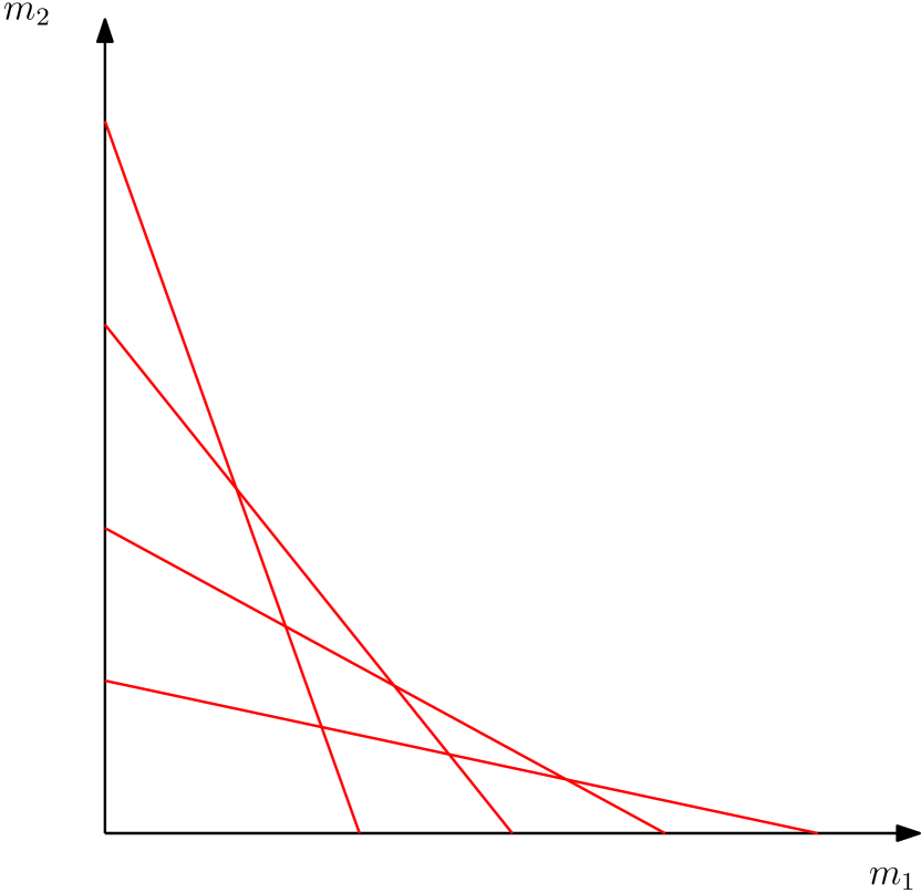
(a)

(b)

(c)

Figure 1. Acceptance region and approximation.

3.2. Effective bandwidths in road traffic

We show how to apply the ideas of the previous subsection to the road traffic context introduced in Section 2. Similar to the telecommunications setting, the objective is to apply input control to a network, so as to bound the probability of exceeding network capacities. The effective bandwidth framework, working with a linear acceptance region, provides a fast and easily implemented procedure for network admission control. The effective bandwidths capture both the mean, variance and other distributional properties of the capacity requirements of the different traffic streams on an arc, and are computed arc-wise, such that additional traffic on a path is simply accepted once it satisfies the control constraints of the arcs making up the path.

First, with similar techniques as in the traditional effective bandwidth literature, we use a Chernoff bound to bound the probability that the capacity of an arc $a_{j}\in A$ is exceeded from above:

$$\log\mathbb{P}(Y_{a_{j}}>C_{a_{j}})\leq\inf_{s\geq 0}\log\big{(}\mathbb{E}[e^{sY_{a_{j}}}]e^{-sC_{a_{j}}}\big{)}=\inf_{s\geq 0}\big{(}\sum_{\begin{subarray}{c}i=1,\dots,I\\ B_{ij}=1\end{subarray}}\log\mathbb{E}[\exp\{s\sum_{k=1}^{M_{i}}D_{ik}\}]\!-\!sC_{a_{j}}\big{)}.$$ (2)

Observing that the expectation in the considered upper bound is the moment-generating function (MGF) of a compound Poisson distribution, we have, for $\gamma>0$,

$$\inf_{s\geq 0}\Big{(}\sum_{\begin{subarray}{c}i=1,\dots,I\\ B_{ij}=1\end{subarray}}r_{P_{i}}(\mathbb{E}[e^{sD_{i1}}]-1)\!-\!sC_{a_{j}}\Big{)}\leq-\gamma\implies\mathbb{P}(Y_{a_{j}}>C_{a_{j}})\leq e^{-\gamma}.$$ (3)

Now, the probability of exceeding the capacity of an arc $a_{j}$, and consequently, the probability of delay around this arc, is small if $\bm{r}$ lies in the acceptance region $R^{\alpha}_{j}$:

$$R^{\alpha}_{j}=\bigcup_{s\geq 0}R_{j,s}^{\alpha},\quad R_{j,s}^{\alpha}=\Bigg{\{}\bm{r}\in\mathbb{R}_{\geq 0}^{I}:\sum_{i=1,\dots,I}B_{ij}r_{P_{i}}\alpha_{i}(s)\leq C_{a_{j}}-\frac{\gamma}{s}\Bigg{\}},\quad\alpha_{i}(s)=(\mathbb{E}[e^{sD_{i1}}]-1)/s.$$

Remark 2.

Note that $\alpha_{i}(s)$ is indeed equivalent to the notion of effective bandwidth as introduced in Kelly and Yudovina (2014). We observe that,

$$\alpha_{i}(s)=\mathbb{E}[e^{sD_{i1}}-1]/s\geq\mathbb{E}[sD_{i1}]/s=\mathbb{E}[D_{i1}],$$

such that the bandwidth is between the mean and peak rate of $Y_{a_{j}}$:

$$\mathbb{E}[Y_{a_{j}}]=\sum_{i=1,\dots,I}B_{ij}r_{P_{i}}\mathbb{E}[D_{i1}]\leq\sum_{i=1,\dots,I}B_{ij}r_{P_{i}}\alpha_{i}(s)<\infty=\sup\{y:\mathbb{P}(Y_{a_{j}}>y)>0\}.$$

Also, comparing the two different notions of effective bandwidths, it can easily be seen that $\alpha_{i}(s)\geq\alpha^{\prime}_{i}(s)$. This is not surprising, as, instead of only protecting against potential high values of $D_{ik}$, we need to protect against high values of $M_{i}$ as well. $\Diamond$

Remark 3.

It is easy to see that (2) is invariant to the distribution of $M_{i}$, in the sense that any distribution over the integers would yield a similar expression for the upper bound. Notably, with $G_{X}(s)=\mathbb{E}\exp\{sX\}$ the MGF of a random variable $X$, the implication in (3) may be replaced by the more general

$$\inf_{s\geq 0}\Big{(}\sum_{\begin{subarray}{c}i=1,\dots,I\\ B_{ij}=1\end{subarray}}\log G_{M_{i}}\big{(}\log G_{D_{i1}}(s)\big{)}\!-\!sC_{a_{j}}\Big{)}\leq-\gamma\implies\mathbb{P}(Y_{a_{j}}>C_{a_{j}})\leq e^{-\gamma},$$

such that the results are easily extended in case $M_{i}$ is another distribution from the family of discrete distributions over the integers for which the MGF is well-defined. $\Diamond$

Similar to the telecommunications setting, the acceptance region $R^{\alpha}_{j}$ is too complex for practical application, i.e., for a given $I$-dimensional vector of stream rates $\bm{r}$ it is hard to decide if there exists an $s_{j}\geq 0$ such that $\bm{r}\in R_{j,s_{j}}^{\alpha}$. Therefore, we approximate the acceptance region $R^{\alpha}_{j}$ by one of the regions $R_{j,s_{j}}^{\alpha}$, whose right boundary is again linear. Then, given the regions $R_{j,s_{j}}^{\alpha}$ and $\varepsilon>0$, the control procedure is simply to allow an average input rate of $r_{P_{k}}(1+\varepsilon)$ instead of $r_{P_{k}}$ if, for all $j\in\{1,\dots,J\}$, the following inequality is satisfied:

$$\sum_{i=1,\dots,I}B_{ij}r_{P_{i}}\alpha_{i}(s_{j})+\varepsilon B_{ij}\alpha_{k}(s_{j})\leq C_{a_{j}}-\gamma/s_{j}.$$ (4)

For each $j=1,\dots,J$, we propose to base the choice of $s_{j}$ (i.e., $R_{j,s_{j}}^{\alpha}$) on the current traffic conditions. Given $\bm{r}$, we let $R_{j,s_{j}}^{\alpha}$ be such that $s_{j}$ attains the infimum in (3). With $s_{j}$ given, the effective bandwidths $\alpha_{j}(s_{j})$ are computed, which may then be stored externally, such that it can be decided rapidly if (4) is satisfied. Note that, as argued in Section 2.2, the application of access control in road networks is a dynamic procedure. On a longer timescale, one should therefore adapt the approximating region to new traffic conditions.

Remark 4.

In the above, $\gamma$ is chosen uniformly for all arcs. We can, however, also work with a bound $\gamma_{a_{j}}>0$ per arc $a_{j}\in A$. This may be preferable if there are arcs in the network for which a congestive setting has a more deteriorating effect on the network than congestive settings on other arcs, as they are e.g. located centrally or have a high degree of neighbouring links. $\Diamond$

One drawback of the described control method is that (3) is not an equivalence statement, making the proposed procedure conservative. In the classical effective bandwidth notion, the acceptance region $R^{\prime}$ is conservative as well, but, in the asymptotic regime, $\mathbb{P}(Y^{\prime}>C^{\prime})\leq e^{-\gamma}$ is approximately the same as $\bm{m}\in R^{\prime}$ (Remark 1). Notably, such a limit argument carries on to the road traffic setting, as can be deduced from the following theorem. This theorem can be obtained as a consequence of the Bahadur-Rao Theorem (Bahadur and Rao, 1960), but also follows straightforward from the direct argument presented below.

Theorem 1.

For $i=1,\dots,I$, let $\{M_{i}(t):t\geq 0\}$ a Poisson process with rate $\lambda_{i}>0$ and $X_{i1},X_{i2},\dots$ i.i.d. random variables independent of $M_{i}$ with $\mathbb{E}[X_{i1}]<c_{i}$, $\mathbb{P}(X_{i1}>c_{i})>0$, and a log-moment generating function that is finite for real values in an open neighbourhood of the origin. Then, with $c=c_{1}+\dots+c_{I}$,

$$\lim_{t\to\infty}\frac{1}{t}\log p_{t}^{c}\equiv\lim_{t\to\infty}\frac{1}{t}\log\mathbb{P}\left(\sum_{i=1}^{I}X_{i1}+\dots+X_{iM_{i}(t)}>ct\right)=\inf_{s>0}\sum_{i=1}^{I}[\lambda_{i}(\mathbb{E}[e^{sX_{i1}}]-1)-c_{i}s].$$

Proof.

The upper bound is an immediate consequence of the Chernoff bound:

$$\lim_{t\to\infty}\frac{1}{t}\log p_{t}^{c} =\lim_{t\to\infty}\frac{1}{t}\log\mathbb{P}\left(\sum_{i=1}^{I}\sum_{k=1}^{M_{i}(t)}X_{ik}>ct\right)\leq\lim_{t\to\infty}\inf_{s>0}\left\{\frac{1}{t}\log\mathbb{E}\Big{[}\exp\big{(}s\sum_{i=1}^{I}\sum_{k=1}^{M_{i}(t)}X_{ik}\big{)}\Big{]}-cs\right\}$$

$$=\lim_{t\to\infty}\inf_{s>0}\left\{\frac{1}{t}\sum_{i=1}^{I}\log\mathbb{E}\Big{[}\exp\big{(}s\sum_{k=1}^{M_{i}(t)}X_{ik}\big{)}\Big{]}-cs\right\}=\inf_{s>0}\sum_{i=1}^{I}[\lambda_{i}\big{(}\mathbb{E}[e^{sX_{i1}}]-1\big{)}-c_{i}s],$$

where the last step follows from (3). For the lower bound, we note that

$$\log p_{t}^{c} \geq\frac{1}{t}\log\mathbb{P}\left(\sum_{i=1}^{I}\sum_{k=1}^{M_{i}(\lfloor t\rfloor)}X_{ik}>c\lfloor t\rfloor\right)+\frac{1}{t}\log\mathbb{P}\left(\sum_{i=1}^{I}\sum_{k=M_{i}(\lfloor t\rfloor)+1}^{M_{i}(t)}X_{ik}\geq c(t-\lfloor t\rfloor)\right).$$

For $M_{i,1},M_{i,2},\dots$ a sequence of i.i.d. $\text{Poisson}(\lambda_{i})$ distributed random variables,

$$\lim_{t\to\infty}\frac{1}{t}\log\mathbb{P}\left(\sum_{i=1}^{I}\sum_{k=1}^{M_{i}(\lfloor t\rfloor)}X_{ik}>c\lfloor t\rfloor\right) =\lim_{t\to\infty}\frac{1}{t}\log\mathbb{P}\big{(}\sum_{i=1}^{I}\sum_{k=1}^{\sum_{l=1}^{\lfloor t\rfloor}M_{i,l}}X_{ik}>c\lfloor t\rfloor\big{)}$$

$$\geq\lim_{t\to\infty}\frac{1}{\lfloor t\rfloor}\log\mathbb{P}\big{(}\sum_{l=1}^{\lfloor t\rfloor}\sum_{i=1}^{I}\sum_{k=1}^{M_{i,l}}X_{ik}>c\lfloor t\rfloor\big{)}$$

$$\equiv\lim_{n\to\infty}\frac{1}{n}\log\mathbb{P}(Z_{1}+\dots+Z_{n}>cn).$$

By Cramérs theorem, letting $M_{i}\sim\text{Poisson}(\lambda_{i})$ and using that $Z_{1},\dots,Z_{n}$ are i.i.d.:

$$\lim_{n\to\infty}\frac{1}{n}\log\mathbb{P}(Z_{1}+\dots+Z_{n}>cn) =\inf_{s>0}\left\{\log\mathbb{E}\big{[}e^{s\sum_{i=1}^{I}\sum_{k=1}^{M_{i}}X_{ik}}\big{]}-cs\right\}=\inf_{s>0}\left\{\sum_{i=1}^{I}[\lambda_{i}\big{(}\mathbb{E}[e^{sX_{i1}}]-1\big{)}-c_{i}s]\right\}.$$

The theorem now follows from noting that for $t\in\mathbb{R}\setminus\mathbb{N}$

$$\frac{1}{t}\log\mathbb{P}\left(\sum_{i=1}^{I}\sum_{k=M_{i}(\lfloor t\rfloor)+1}^{M_{i}(t)}X_{ik}>c(t-\lfloor t\rfloor)\right) \geq\frac{1}{t}\min_{u\in(0,1]}\log\mathbb{P}\left(\sum_{i=1}^{I}\sum_{k=1}^{M_{i}(u)}X_{ik}>cu\right)\overset{t\to\infty}{\to}0.$$

∎

4. Numerical Experiments

Now that we have shown how the notion of effective bandwidths can be used to regulate traffic streams in road networks, so as to avoid network congestion, we perform a set of numerical experiments in order to assess the performance of the proposed policies. Specifically, we demonstrate that capacity violations are indeed rare, and that the waiting costs at the boundaries of the network are typically of a smaller scale than the incurred costs of such violations. In the experiments, the policy that follows from the effective bandwidth framework is denoted with EB($\gamma$), where $\gamma>0$ such that the probability of capacity violation is upper bounded by $e^{-\gamma}$ (see (3)).

We compare the performance of the effective bandwidth framework, in terms of waiting times and number of capacity violations, to three other input rate control algorithms, which serve as natural benchmarks. As a first benchmark, we use the procedure that simply allows all vehicles in the network at all times, which will be called ’No Control’ (abbreviated to NC). The second benchmark does incur waiting costs at the boundary, as it will not allow the expected capacity needs on the links to exceed the link capacities, i.e., $\mathbb{E}[Y_{a_{j}}]<C_{a_{j}}$ for all $a_{j}\in A$. This procedure will be called ’Expected Needs’, and the corresponding policies are abbreviated with EN. The third benchmark, called ’Random Needs’, takes the random nature of capacity needs into account, and only allows the current input rate when, for some chosen $\alpha>0$ and all $a_{j}\in A$,

$$\mathbb{E}[Y_{a_{j}}]+\alpha\sqrt{\text{Var}\left(Y_{a_{j}}\right)}<C_{a_{j}}.$$

The corresponding procedure is abbreviated to RN($\alpha$). When aiming for a similar guarantee as in the EB-framework, a natural way to calibrate $\alpha$ is to use a normal approximation and set $\alpha\equiv z_{\exp\{-\gamma\}}$, with, for $Z\sim N(0,1)$ and any $\beta>0$, $z_{\beta}$ such that $\mathbb{P}(Z\geq z_{\beta})=\beta$. For any $\gamma>0$, we will denote such a calibration as $\alpha_{\gamma}$.

Experiment 1 examines the impact of the different policies on a network consisting of a single link, whereas Experiment 2 considers networks of larger size. For the experiments we implemented the networks and policies in Wolfram Mathematica 12.0 on an Intel® Core™ i7-8665U 1.90GHz computer.

Experiment 1

For illustration purposes, we consider a network that consists of a single link, with a capacity of 50. The amount that one vehicle contributes to the occupied capacity is modeled as $D\sim$ Hyperexponential($\bm{p},\bm{\lambda}$), with $\bm{p}=(0.7,0.3)$ and $\bm{\lambda}=(3/2,9/16)$. This could ge.g. represent a traffic stream for which any vehicle is a car with 70% probability and with 30% probability it is a truck; cars and trucks occupying a capacity of 2/3 and 16/9, respectively, such that the expected capacity needs of a single vehicle equal 1. We consider a rush-hour setting, in which, starting at a low mean demand at time 0 (i.e., the time the rush hour initiates), the mean input rate of the link first monotonically increases, and then monotonically decreases, after which the rush hour has passed, and the mean demand stays constant. Specifically, in this experiment, we consider the mean traffic demand to evolve as in Figure 2. For this mean demand curve, Figure 2 plots the (simulated) probability of a capacity violation at several points in time, in case there is no input rate control (policy NC). Setting our goal to keep this probability below $e^{-4}$, we evaluate the network performance for the policies EN, RN($\alpha_{4}$) and EB(4).

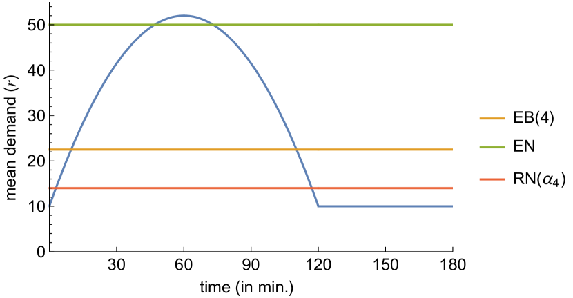
(a) Mean traffic demand $r$ as function of time in a rush hour setting, together with the maximum input rates of three control policies.

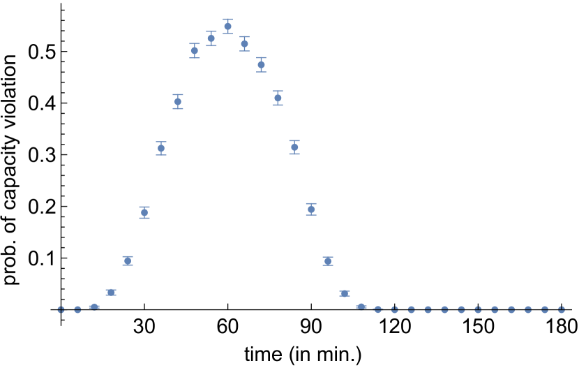
(b) Probability of capacity violation as a function of time for policy NC.

Figure 2. Example of the mean demand during rush hour on a single link.

Figure 2 also shows the maximum input rates for the different control policies. For any of the control policies, the probability of capacity violation can be read off the right hand graph, as long as the mean traffic demand (in the right hand graph) has not yet reached the imposed threshold. For the EN-policy this yields a probability larger than 0.45 that a capacity violation occurs during the peak period of the rush hour. For the NC-policy, allowing all traffic demand into the network, this probability is larger than 0.5. EB(4) and RN($\alpha_{4}$) are more conservative, and limit access at an earlier stage. Recall that, the latter two policies target at a probability of capacity violations of $e^{-4}\approx 0.02$ (for RN this is by approximation using a normal distribution, and for EB it is a bound).

Our aim is to avoid the high delays caused by capacity violations, at the expense of some additional delay on the boundaries of the network. We assess the gains of this approach in terms of a proxy for the total delay vehicles experience during their travel, using the following simulation approach. First, we discretize time in steps of size $\delta>0$, and view the evolution of traffic as a queueing model that consists of a waiting area of infinite size at the starting node of the link, which we will refer to as the buffer, and a FCFS em queue on the link itself. The buffer and queue size at time $t$ are denoted by $B(t)$ and $Q(t)$, respectively. At each time step $t=\delta m$, the mean traffic demand $r_{t}$ is obtained from the area below the function in Figure 2 between $\delta(m-1)$ and $\delta m$. The control policy then decides how much of $B(t\!-\!\delta)$ and $r_{t}$ is offered to the queue. Let $\bar{\rho}_{t}$ be the maximum mean flow rate the control policy allows at time $t$. Then, a mean flow rate of $\bar{r}_{t}\equiv\min\{\bar{\rho}_{t},B(t\!-\!\delta)+r_{t}\}$ is admitted to the queue, such that $B(t)=B(t\!-\!\delta)+r_{t}-\bar{r}_{t}$.

Whenever, at time $t=\delta m$, a mean traffic load of $\bar{r}_{t}$ enters the link, the corresponding number of vehicles is simulated, and they are placed in the queue. For each of these vehicles, a sample of their capacity needs yields their service requirement. The amount of capacity needs that the server is able to process between $\delta m$ and $\delta(m+1)$ is given through a function $c(\cdot)$, which takes the total capacity needs in the queue at time $\delta m$ as input. The shape of the function is chosen to represent the impact of high capacity needs on the driveable speeds. That is, whenever the capacity needs are less than the capacity on the link, vehicles are effectively able to drive the free-flow speed, represented by the fact that all capacity can be processed. Whenever the capacity needs exceed the link capacity, the attainable speeds are much lower, which is represented by the fact that $c(\cdot)$ outputs a value that is far less than the link capacity. Specifically, in this example, we let

$$c(y)\equiv\begin{cases}y&y\leq 50\delta\\ \max\{10\delta,100\delta\!-\!y\}&y>50\delta.\end{cases}$$ (5)

Note that we multiply the numbers by $\delta$, to account for the fact that we look at time windows of size $\delta$. Furthermore, under congested conditions, we impose a strictly positive service rate, to make sure that, for low arrival rates, the model is able to recover from these congested conditions at a future time point.

With the procedure described above we obtain a proxy for the total delay in the network in the following way. At each time $t$, an approximation for the total number of customers in the system is given through the sum of $B(t)$ and the number of vehicles in the queue. Computing this sum for each simulation run and each point in time, we obtain an approximation for $\tilde{L}$, the average number of customers in the system. Moreover, averaging over the mean demands $r_{t}$ of the different time steps yields an estimate $\tilde{r}$ for the average arrival rate. Then, with Little’s law, we obtain the proxy $\tilde{L}/\tilde{r}$ for the delay vehicles in the network experience. The proxies for different control procedures, in the setting described above, with the time range of Figure 2, $B(0)=0$, $Q(0)=0$, and $\delta=1$ min, are given in Table 1. These proxies reveal that the delay for the NC- and EC-policy is of the same order, which can be explained by the fact that EN solely limits access in the peak of the rush hour. The delay under EB(4) is significantly lower, whereas the delay under RN($\alpha_{4}$) is of very high order.

	NC	EN	RN($\alpha_{4}$)	EB(4)
Delay estimate (in min.)	49.43	49.41	66.57	41.97

Table 1. Estimates for the delays vehicles experience in a single-link network under different input rate control policies, for the mean demand curve of Figure 2.

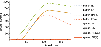
Figure 3. Average buffer and queue size as a function of time, for four different control policies.

The differences in experienced delays as presented in Table 1 can also be observed in Figure 3, which shows the buffer and average queue size for the four policies as a function of time. Note that the mean demand arriving at the buffer is deterministic, such that the buffer size, in terms of mean demand, is a deterministic quantity. The number of vehicles entering the queue being a random variable, the queue size is a random quantity, whose average is determined with 10.000 simulations. Again, we observe that there is little difference between the NC- and EN-policies, because both allow a high mean demand onto the link, such that the buffer stays relatively empty. However, on the link itself, due to violations of the link capacity, the traffic becomes, and stays, highly congested.

Figure 3 shows that both EB(4) and RN($\alpha_{4}$) indeed succeed in avoiding high delays on the link, as the queue sizes under both policies remain of a very small scale. Under EB(4), the demand in the buffer grows during the rush hour period, but as there is no congestion on the link, the total delay is still much lower than in the NC- or EN-regime. This is not the case for the RN($\alpha_{4}$)-policy: being very conservative, the buffer size is such that the total delay exceeds the NC- and EN-regime. However, it is important to remark that there is a difference between the delay vehicles experience on the boundaries and inside the network. That is, by using Intelligent Transportation Systems, drivers may request their route from e.g. their home, and learn when they will be granted access to the network from there, such that waiting at the boundaries does not automatically yield wasted time for the affected drivers. This in contrast to waiting inside the network, which, moreover, results in additional CO₂ emissions.

Figure 4. A linear network with $m$ links.

Experiment 2

To examine the impact of capacity violations in larger networks, we consider the linear network of Figure 4, and vary $m$, the number of links of which the network consists. The network has a single traffic stream, with vehicles wanting to travel from the left node to the right node. For this stream, we consider the same mean demand curve and the same capacity needs characteristics as in Exp. 1. Moreover, we let all link capacities equal 100, except for the last link, whose capacity is chosen to be 50.

Now, to compute proxies for the delays vehicles experience under the control procedure, we discretize time in steps of size $\delta>0$, and again view the evolution of traffic as a queueing system, with a single buffer of infinite size at the starting node, and FCFS queues on each of the $m$ links. The buffer dynamics are similar to those in Exp. 1, with the vehicles that are allowed into the network arriving at the queue that corresponds to link 1. These vehicles visit the queues consecutively: traffic that has been served by the queue of link $i$ ($1\leq i\leq m-1$) is inserted in the queue of link $i+1$. If a vehicle has been served by the queue of link $m$, it leaves the system. Now, by summing, for each simulation, the vehicles in all queues at every time step, an application of Little’s law again yields the order of travel time delays.

Let $c_{i}(\cdot)$ be the amount of capacity needs that the server at the queue on link $i$ is able to process. With $\bm{y}$ a vector of the capacity needs on each link, $y_{i}$ denoting its $i$-th coordinate, and $c(\cdot)$ as in (5), we let $c_{m}(\bm{y})=c(y_{m})$. Then, to capture the fact that traffic jams propagate through the network, we let, for any link $1\leq i\leq m-1$, the function $c_{i}(\cdot)$ explicitly depend on the total capacity needs in its queue, as well as the total capacity needs in the next queue. That is, the shape of the function represents that if the next queue is highly congested, new traffic is not able to enter this queue, and has to stay in its current queue. Specifically, allowing not more than $u_{i}\equiv 190\delta$ per time step into queue $i$ for any $1\leq i\leq m-1$, and not more than $u_{m}\equiv 90\delta$ per time step into queue $m$,

$$c_{i}(\bm{y})\equiv\begin{cases}\min\{u_{i+1}-y_{i+1}+c_{i+1}(\bm{y}),y_{i}\}&y_{i}\leq 100\delta\\ \min\{u_{i+1}-y_{i+1}+c_{i+1}(\bm{y}),\max\{10\delta,200\delta\!-\!y_{i}\}\}&y_{i}>100\delta.\end{cases}$$

With $c_{m}(\bm{y})$ known, the amount of vehicles that are served in each queue can be computed recursively.

	NC	EN	RN($\alpha_{4}$)	EB(4)
$m=5$	49.36	48.99	68.49	45.01
$m=10$	49.98	49.73	70.84	48.73
$m=20$	55.43	56.52	75.30	54.81
$m=30$	62.23	61.82	79.49	60.43

Table 2. Estimates for the delays vehicles experience in the network of Fig. 4, under different input rate control policies, for the mean demand curve of Figure 2.

The proxies under different input rate control schemes are presented in Table 2, and are, naturally, increasing functions in $m$. Just as in Exp. 1, the NC- and EN-policy behave relatively similar. Their high delay values are caused by the fact that the buffer is relatively empty throughout the complete time window. EB(4) outperforms these policies, but the high buffer value causes quite high delays, especially for large values of $m$. However, as argued above, waiting at the boundaries of the network is significantly different from waiting within the network, as it is not directly a time waste, and has no negative environmental consequences. A similar argument can be made for RN($\alpha_{4}$), which has the highest delays, but may still be preferred over NC- and EN.

5. Concluding remarks

In this work, we used a compound Poisson process to describe the random part of the road capacity that is effectively taken by the traffic streams using that road. To avoid that, in a given road network, link capacities are exceeded, we constructed an input rate control policy that takes the randomness of these capacity needs into account. This policy guarantees an upper bound on the capacity-violation probability, and is based on the notion of effective bandwidths as originally introduced in the telecommunications context. Numerical experiments demonstrated that, typically, the total delay in the network is of a smaller scale than the delay would be without access control, or with a policy that only takes expected capacity needs into account.

There are a few natural ways in which our modeling procedure may be extended, towards which future work could be specified. For example, in the current procedure, when determining the input role control, the location of the vehicles on the paths does not play a role. Specifically, if given access to the network, in our model setting, a demand increase on a given path will instantaneously lead to an increase in the capacity needs on all links on this path. In reality, however, there is a time-component, and an increase in traffic demand at the boundary will only lead to an increase in capacity needs on further links at later points in time.

The aim or our control procedure was to limit the negative consequences of capacity violations. Although our procedure does describe the traffic demand that is allowed into the network, it does not consider the fairness in terms of waiting time. That is, if the demand on a single link consists of two traffic streams with the same characteristics, instead of allowing a part of both streams, our procedure may only allow one of the streams. Therefore, in terms of practical operationalization, a potential suggestion for future research would be to adapt our procedure so as to meet certain fairness guarantees.

An interesting application of our work would be the identification of network bottlenecks. Since our procedure can identify, for a given demand, the set of links whose capacities have a significant probability to be violated, this will provide an impression of the bottlenecks in the network. Notably, with the characteristics of recurrent traffic demand well known, this may be helpful in deciding on future changes in network infrastructure.

Declarations

Funding

This research is funded by the NWO Gravitation project networks under grant no. 024.002.003.

Competing interests

The authors have no competing interests to declare that are relevant to the content of this article.

References

- (1)
- Adnan (2014) Adnan, M. (2014), ‘Passenger car equivalent factors in heterogenous traffic environment-are we using the right numbers?’, Procedia Engineering 77, 106–113.
- Angelidakis et al. (2013) Angelidakis, H., Fotakis, D. and Lianeas, T. (2013), Stochastic congestion games with risk-averse players, in ‘Algorithmic Game Theory, SAGT 2013, Lecture Notes in Computer Science, vol 8146.’, pp. 86–97.
- Arnott et al. (1990) Arnott, R., de Palma, A. and Lindsey, R. (1990), ‘Economics of a bottleneck’, Journal of Urban Economics 27(1), 111–130.
- Bahadur and Rao (1960) Bahadur, R. R. and Rao, R. R. (1960), ‘On deviations of the sample mean’, The Annals of Mathematical Statistics 31(4), 1015 – 1027.
- Bonald and Roberts (2007) Bonald, T. and Roberts, J. (2007), ‘Scheduling network traffic’, ACM SIGMETRICS Perform. Eval. Rev. 34(4), 29–35.
- Cominetti et al. (2019) Cominetti, R., Scarsini, M., Schröder, M. and Stier-Moses, N. E. (2019), Price of Anarchy in Stochastic Atomic Congestion Games with Affine Costs, in ‘Proceedings of the 2019 ACM Conference on Economics and Computation’, EC ’19, Association for Computing Machinery, pp. 579–580.
- Daganzo (1994) Daganzo, C. F. (1994), ‘The cell transmission model: A dynamic representation of highway traffic consistent with the hydrodynamic theory’, Transportation Research Part B: Methodological 28(4), 269–287.
- Daganzo (1995) Daganzo, C. F. (1995), ‘The cell transmission model, part II: Network traffic’, Transportation Research Part B: Methodological 29(2), 79–93.
- Elwalid and Mitra (1993) Elwalid, A. I. and Mitra, D. (1993), ‘Effective bandwidth of general Markovian traffic sources and admission control of high speed networks’, IEEE/ACM Transactions on Networking 1(3), 329–343.
- Ghazanfari et al. (2021) Ghazanfari, S., van Leeuwen, D., Ravner, L. and Queija, R. N. (2021), ‘Commuter behavior under travel time uncertainty’, Performance Evaluation 148.
- Gibbens and Hunt (1991) Gibbens, R. J. and Hunt, P. J. (1991), ‘Effective bandwidths for the multi-type UAS channel’, Queueing Systems 9, 17–27.
- Hui (1988) Hui, J. Y. (1988), ‘Resource allocation for broadband networks’, IEEE Journal on Selected Areas in Communications 6(9), 1598–1608.
- Jabari and Liu (2012) Jabari, S. E. and Liu, H. X. (2012), ‘A stochastic model of traffic flow: Theoretical foundations’, Transportation Research Part B: Methodological 46(1), 156–174.
- Kelly (1991) Kelly, F. P. (1991), ‘Effective bandwidths at multi-class queues’, Queueing Systems 9, 5–15.
- Kelly and Williams (2010) Kelly, F. P. and Williams, R. J. (2010), Heavy traffic on a controlled motorway, in ‘Probability and Mathematical Genetics: Papers in Honour of Sir John Kingman’, p. 416 – 445.
- Kelly and Yudovina (2014) Kelly, F. and Yudovina, E. (2014), Stochastic Networks, Cambridge University Press.
- Koole (2013) Koole, G. G. M. (2013), Call Center Optimization, MG Books.
- Kovács (2016) Kovács, P. (2016), Stochastic models for road traffic control, PhD thesis, University of Amsterdam.
- Levering et al. (2021) Levering, N., Boon, M., Mandjes, M. and Núñez-Queija, R. (2021), ‘A Framework for Efficient Dynamic Routing under Stochastically Varying Conditions’.
- Lighthill and Whitham (1955) Lighthill, M. J. and Whitham, G. B. (1955), ‘On kinematic waves II. A theory of traffic flow on long crowded roads’, Proceedings of the Royal Society of London. Series A, Mathematical and Physical Sciences 229(1178), 317–345.
- Mandjes and Storm (2021) Mandjes, M. and Storm, J. (2021), ‘A diffusion-based analysis of a multiclass road traffic network’, Stochastic Systems 11(1), 60–81.
- Nikolova and Stier-Moses (2011) Nikolova, E. and Stier-Moses, N. E. (2011), Stochastic selfish routing, in ‘Algorithmic Game Theory, SAGT 2011, Lecture Notes in Computer Science, vol 6982.’, pp. 314–325.
- Papageorgiou and Kotsialos (2002) Papageorgiou, M. and Kotsialos, A. (2002), ‘Freeway ramp metering: An overview’, IEEE Transactions on Intelligent Transportation Systems 3(4), 271–281.
- Qu et al. (2017) Qu, X., Zhang, J. and Wang, S. (2017), ‘On the stochastic fundamental diagram for freeway traffic: Model development, analytical properties, validation, and extensive applications’, Transportation Research Part B: Methodological 104, 256–271.
- Richards (1956) Richards, P. I. (1956), ‘Shock waves on the highway’, Operations Research 4(1), 42–51.
- Shaaban et al. (2016) Shaaban, K., Khan, M. A. and Hamila, R. (2016), Literature review of advancements in adaptive ramp metering, in ‘Procedia Computer Science’, Vol. 83, Elsevier, pp. 203–211.
- Sharma and Biswas (2021) Sharma, M. and Biswas, S. (2021), ‘Estimation of passenger car unit on urban roads: A literature review’, International Journal of Transportation Science and Technology 10(3), 283–298.
- Vickrey (1969) Vickrey, W. S. (1969), ‘Congestion theory and transport investment’, The American Economic Review 59(2), 251–260.