Migrate Demographic Group For Fair GNNs

Abstract.

Graph Neural networks (GNNs) have been applied in many scenarios due to the superior performance of graph learning. However, fairness is always ignored when designing GNNs. As a consequence, biased information in training data can easily affect vanilla GNNs, causing biased results toward particular demographic groups (divided by sensitive attributes, such as race and age). There have been efforts to address the fairness issue. However, existing fair techniques generally divide the demographic groups by raw sensitive attributes and assume that are fixed. The biased information correlated with raw sensitive attributes will run through the training process regardless of the implemented fair techniques. It is urgent to resolve this problem for training fair GNNs. To tackle this problem, we propose a brand new framework, FairMigration, which can dynamically migrate the demographic groups instead of keeping that fixed with raw sensitive attributes. FairMigration is composed of two training stages. In the first stage, the GNNs are initially optimized by personalized self-supervised learning, and the demographic groups are adjusted dynamically. In the second stage, the new demographic groups are frozen and supervised learning is carried out under the constraints of new demographic groups and adversarial training. Extensive experiments reveal that FairMigration balances model performance and fairness well.

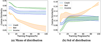
Figure 1. The change curve of group similarity distribution of vanilla GCN on three datasets. The bold lines with the same color indicate the mean(std) of two group similarity distributions on the same dataset, respectively. The shaded areas indicate the group similarity distribution difference. The wider the shaded area on the y-axis, the larger the similarity difference between groups.

1. Introduction

In recent years, graph neural networks (GNNs) have attracted much attention due to the potent ability to convey data in a graph-structured manner. In many real-world scenarios, including node classification (Kipf and Welling, 2016; Veličković et al., 2017; Xu et al., 2018a, b; Gasteiger et al., 2018; Hamilton et al., 2017), community detection (Shchur and Günnemann, 2019; Sun et al., 2021; Qiu et al., 2022), link prediction (Zhang and Chen, 2018; Cai et al., 2021; Long et al., 2022) and recommendation systems (Wang et al., 2022a; Gwadabe and Liu, 2022; Yin et al., 2019), have been applied to GNNs. The GNN aggregates the messages delivered by neighbors to obtain the embedding of nodes, edges, or graphs. The key to the powerful expression ability of GNN lies in extracting the attribute features and the structural features in the graph structure data at the same time.

Recently, fairness has become a high-profile issue. Several recent studies have shown that AI models may produce biased results for specific groups or individuals divided by some particular sensitive attributes, such as race, age, gender, etc. The biased algorithms have resulted in some horrible cases. An American judicial system’s algorithm erroneously predicts that African Americans will commit twice as many crimes as whites. Amazon found that its recruitment system was biased against female candidates, especially in tech positions (Mehrabi et al., 2021). The further application of AI models will be severely constrained if the fairness issue cannot be satisfactorily addressed.

In deep learning, there have been some works that try to resolve the fairness issue. Fairboosting (Yu et al., 2021) aims at resolving the low recognition rate of mask-wearing faces in East Asia, using the masking method to generate masking faces, balancing the data with resampling, and proposing a symmetric arc loss to improve recognition accuracy and fairness. To improve counterfactual token fairness in text classification and connect robustness and fairness, Garg et al. (Garg et al., 2019) propose three methods: blinding, counterfactual enhancement, and counterfactual logical pairing. Wang et al. (Wang et al., 2023) effectively promote fairness by minimizing the mutual information between the semantics in the generated text sentences and the polarity of their demographics. Jalal et al. (Jalal et al., 2021) define several intuitive concepts about group fairness for image generation with uncertain-sensitive properties, and explores these concepts’ incompatibilities and trade-offs.

However, fair deep learning methods seldom take samples’ interaction into account. Therefore, the fair deep learning techniques are not applicable to graph data (Choudhary et al., 2022). There are also several efforts to address the fairness issue in GNNs. FairGNN (Dai and Wang, 2021) employs adversarial training to prevent GNNs from leaking sensitive information during message passing. Edits (Dong et al., 2022) preprocesses attributes and topologies to reduce biased information. Although these methods solve the fairness issue for GNNs to a certain extent, they are still restricted to fixed sensitive information. The existing fair GNN strategies are unable to decouple the original sensitive attribute with prediction due to a lack of effective solutions to the biased information included in raw sensitive attributes.

The biased results generated by vanilla GNN can be attributed to a variety of factors. To begin with, when labeling the data, it will ineluctably be influenced by subjective elements and resemble previous historical data (Beutel et al., 2017; Creager et al., 2019; Dwork et al., 2012; Dai and Wang, 2021). These biased properties are introduced into graph neural networks during training and displayed in the outcomes. Second, GNNs correlate each dimension feature, including sensitive attributes, with the prediction result (Dong et al., 2021; Wang et al., 2022c; Dong et al., 2022; Ma et al., 2022). For different groups divided by sensitive attributes, the tightness and accuracy of the correlation between sensitive attributes and predict labels may differ enormously. For example, when a group’s label distribution is extremely unbalanced, the GNNs tend to predict this group to the majority of the group’s labels and strongly correlate the group’s sensitive attribute with the predicted label. On the contrary, if a group’s label distribution is relatively uniform, the GNNs will tend to give a lower weight to the sensitive attribute of the group and make random predictions during training, resulting in poor performance in the group. In addition, the topology of the graph also introduces biased information during message passing. In a homogeneous graph, two nodes directly connected usually have the same or similar attribute characteristics. When smoothing the graph data by GNN will make the groups more concentrated internally and more opposed and exclusive between groups (Jiang et al., 2022; Kipf and Welling, 2016; Wang et al., 2022c). Finally, sensitive attributes are considered immutable by existing fair algorithms on GNNs. Under such circumstances, the bias in the initial data will always impede the model training process, regardless of how the model is improved. When training GCN (Kipf and Welling, 2016) on the three datasets, the change tendency of group similarities is illustrated in Figure 1. It is evident that the distribution of group similarity between two groups diverges increasingly with fixed sensitive attributes, leading to a biased prediction toward one group.

In this paper, we propose a novel model, FairMigration, for the fairness issue of GNNs. FairMigration is an additive method realizing the group migration, which could break the limitation of static sensitive attributes and gradually remove the biased information contained in the original data in the training of the GNNs. The training of FairMigration is divided into two stages. In the first stage, the encoder is trained by personalized self-supervised learning and learns the embeddings of nodes. Based on group similarity distribution, outliers in one group are transferred to another group. After the first stage of training, the encoder is preliminarily trained and the migrated groups division is acquired. In the second stage, the encoder and the classifier are optimized by supervised learning under the condition of the new pseudo-demographic groups and adversarial training. Our contributions are summarized below:

• To our knowledge, we first point out that the biased information contained in static sensitive attributes will always exist in training for fair GNNs.

• We propose a model with group migration to address the problem of biased information contained in fixed sensitive attributes.

• Extensive experiments verify the effectiveness of the proposed method in this paper.

2. Related Work

2.1. Graph Neural Networks

Many Graph Neural Networks (GNNs) have been proposed to learn the representation of graph structure data. GCN (Kipf and Welling, 2016) uses the first-order approximation of Chebyshev’s polynomial as the aggregation function of message passing, GAT (Veličković et al., 2017) uses the attention mechanism to assign message weight for aggregation, GIN (Xu et al., 2018a) aggregates messages with a summation function. Jump Knowledge (JK) (Xu et al., 2018b) passes the output of each layer of the graph neural network to the final layer for aggregation. APPNP (Gasteiger et al., 2018) combines personalized PageRank with GCN to aggregate the information of high-order neighbors. GraphSAGE (Hamilton et al., 2017) generalizes GCN to inductive tasks, learning a function that aggregates the representation of known neighbors.

2.2. Fairness In Deep Learning

The methods of solving the fairness problem in DL can be categorized into three types: pre-processing, in-processing treatment, and post-processing (Mehrabi et al., 2021).

The pre-processing methods perform debiasing operations on the data before training, such as modifying attributes and regenerating labels. Lahoti et al. (Lahoti et al., 2019) create fair representation before training through external knowledge. Ustun et al. (Ustun et al., 2019) construct a debiased classifier through recursive feature picking. Mehrotra et al. (Mehrotra and Celis, 2021) denoise sensitive attributes to reduce gender and racial bias.

The in-processing methods alleviate the bias of the model when training. Chai et al. (Chai and Wang, 2022) dynamically adjust the weights of the loss function during training. FairSmooth (Jin et al., 2022) train classifiers in each group separately and then aggregates classifiers by Gaussian smooth.

The post-processing methods modify the output to obtain debiased results. Lohia et al. (Lohia et al., 2019) use an individual bias detector for prioritizing data samples in a bias mitigation algorithm. Mishler et al. (Mishler et al., 2021) have developed a post-processing predictor that estimates, expands and adjusts previous post-processing methods through a dual robust estimator. Putzel et al. (Putzel and Lee, 2022) modify the predictions of the black-box machine learning classifier for fairness in multi-class settings.

Table 1. Notation Statements Table

notation	statement
$\mathcal{G}(\mathbf{A},\mathbf{X})$	original graph
$\mathbf{X}$	attribute matrix
$\mathbf{A}$	adjacency matrix
$\mathbf{Y}$	ground-truth labels
$\tilde{\mathbf{Y}}$	predicted labels
$\mathbf{S}$	sensitive attribute vector
$\mathbf{U}$	attribute matrix without sensitive attribute
$\tilde{\mathcal{G}}_{j}(\mathbf{A},\tilde{\mathbf{X}}_{j})$	j-th augmented graph
$\tilde{\mathbf{X}}_{j}$	j-th augmented attribute matrix
$\mathbf{Z}$	embedding of graph $\mathcal{G}$
$\mathbf{Z}[i,:]$	i-th row of $\mathbf{Z}$
$\mathbf{Z}_{j}$	embedding of j-th augmented graph
$\mathbf{Z}_{j}[i,:]$	i-th row of $\mathbf{Z}_{j}$
$\mathbf{X}^{rec}$	reconstructed attribute matrix
$\mathbf{U}^{rec}$	reconstructed attribute matrix without sensitive attribute
$\mathbf{S}^{rec}$	reconstructed sensitive attribute vector
$\mathbf{S}_{i}^{rec}$	reconstructed sensitive attribute of i-th node
$\mathbf{P}$	current pseudo attribute matrix
$\mathbf{T}_{i}$	prototype of i-th group
$\mathbf{Q}$	group similarity distribution matrix
$\mu_{\mathbf{P}_{i}},\sigma_{\mathbf{P}_{i}}$	mean and std of similarity of group ${\mathbf{P}_{i}}$
$\mathbf{O}$	outlier set
$\alpha,\gamma,\delta,\lambda$	hyperparameter

2.3. Fairness In Graph Neural Networks

There have been some attempts to address the group-level fairness issues of graph neural networks. FairDrop (Spinelli et al., 2021) prevents unfair information transmission in graph neural networks by randomly masking some edges. GRADE (Wang et al., 2022b) improves the fairness of GNNs through edge interpolation generation and attribute masking. Köse et al. (Köse and Shen, 2021) have developed four new graph enhancement methods to achieve fair graph contrastive learning. FairAug (Kose and Shen, 2022) reduces biased results in graph contrastive learning through adaptive data augmentation. FairRF (Zhao et al., 2022) explores the issue of training fair GNNs under the condition of unknown sensitive attributes. FairGNN (Dai and Wang, 2021) uses adversarial training to prevent the leakage of sensitive attributes. Nifty (Agarwal et al., 2021) adopts a counterfactual augmented siamese network and regularization of model parameters meeting the Lipschitz condition for debiasing. Edits (Dong et al., 2022) constrains the Wasserstein distance of attributes between groups, and then augments topology based on preprocessed attributes to output debiased results. GUIDE (Song et al., 2022) proposes a new method for measuring group-level fairness. FairVGNN (Wang et al., 2022c) adopts adversarial training, feature masking, and gradient cropping to reduce bias. FMP (Jiang et al., 2022) resists topology bias by constraining the distance of raw attributes and the embeddings. The above algorithms train fair GNN under the fixed sensitive attributes, encountering bottleneck of fairness improvement.

3. Preliminary

In this section, the notations of this paper will be illustrated and the problem definition will be given.

3.1. Notations

Given a graph $\mathcal{G}(\mathbf{A},\mathbf{X})$, $\mathbf{A}\in\mathbb{R}^{N\times N}$ denotes the adjacency matrix of $\mathcal{G}$, and $\mathbf{X}\in\mathbb{R}^{N\times K}$ denotes the attribute matrix of $\mathcal{G}$. The sensitive attribute vector is denoted by $\mathbf{S}\in\mathbb{R}^{N}$, which is a column of the attribute matrix $\mathbf{X}$. $\mathbf{U}\in\mathbb{R}^{N\times{(K-1)}}$ denotes the attribute matrix removed $\mathbf{S}$ from $\mathbf{X}$. $\mathcal{G}(\mathbf{A},\mathbf{X})$ can be augmented to the j-th view $\tilde{\mathcal{G}}_{j}(\mathbf{A},\tilde{\mathbf{X}}_{j})$, where $\tilde{\mathbf{X}}_{j}$ is the corresponding augmented attribute matrix. GNN learns the representation of nodes, mapping the graph $\mathcal{G}$ into the embedding matrix $\mathbf{Z}\in\mathbb{R}^{N\times d}$. Similarly, the embedding matrix of graph $\tilde{\mathcal{G}}_{j}$ is denoted by $\mathbf{Z}_{j}\in\mathbb{R}^{N\times d}$. The decoder GNN recovers the attribute matrix from $\mathbf{Z}$. The reconstructed attribute matrix is denoted by $\mathbf{X}^{rec}\in\mathbb{R}^{N\times K}$. The reconstructed sensitive vector is denoted by $\mathbf{S}^{rec}\in\mathbb{R}^{N}$. The matrix, removing $\mathbf{S}^{rec}$ from $\mathbf{X}^{rec}$, is denoted by $\mathbf{U}\in\mathbb{R}^{N\times{(K-1)}}$. Our method involves a group migration module. The corresponding notation mainly includes the current pseudo attribute matrix $\mathbf{P}\in\mathbb{R}^{N}$, the group similarity distribution matrix $\mathbf{Q}\in\mathbb{R}^{N}$, the prototype of i-th group $\mathbf{T}_{i}\in\mathbb{R}^{d}$ and the outlier set $\mathbf{O}$. For convenience, all the important notations are listed in Table 1.

3.2. Problem Definition

The fairness issue can be divided into two levels: group-level fairness and individual-level fairness. The group-level fairness emphasizes fairness between different groups and treat every group equally. Individual fairness emphasizes the fairness between individuals, and reduces the prediction difference of similar individuals. This paper mainly focuses on single-value binary group-level fairness, which is measured by the difference in the probability of being predicted for a particular label on two groups.

4. Method

In this section, the proposed model, FairMigration will be introduced in detail. FairMigration consists of two training stages. In the first stage (self-supervised learning stage), FairMigration constructs pseudo-demographic groups by group migration based on similarity while initially optimizing the encoder using self-supervised learning based on counterfactual fairness. The division of pseudo-demographic groups is expected to correspond to the ground-truth labels, rather than the original sensitive attributes. The obtained pseudo-demographic groups are applied to the model’s training in the supervised learning stage. In the second stage (supervised learning stage), in addition to the cross-entropy, the adversarial training and the pseudo-demographic group based distance restriction are added to further increase fairness.

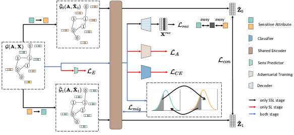
Figure 2. Framework of FairMigration. The workflow of Self-Supervised Learning (SSL) stage only is colored black. The workflow of Supervised Learning (SL) stage only is colored red. The workflow of both SSL stage and SL stage is colored blue. At SSL stage, FairMigration optimizes the encoder by personalized self-supervised learning and migrates the demographic groups. At SL stage, FairMigration optimizes the encoder and the classifier under the constraints of migrated groups and adversarial training.

4.1. Self-Supervised Learning Stage

The target of FairMigration is to improve the fairness of the graph neural network through group migration. Augmentation of the sensitive attributes during the self-supervised learning stage meets with the downstream tasks. In addition, the encoder can be optimized preliminarily. Therefore, we choose sensitive attributes flip as the augmentation strategy for self-supervised training.

4.1.1. Counterfactual fairness augmentation

Given a graph $\mathcal{G}(\mathbf{A},\mathbf{X})$, $\mathbf{A}$ is the adjacency matrix, and $\mathbf{X}$ is the attribute matrx. Two augmented views of $\mathcal{G}$, generated by setting all the sensitive attributes $\mathbf{S}$ as 0 and 1, can be annotated as $\tilde{\mathcal{G}}_{0}(\mathbf{A},\tilde{\mathbf{X}}_{0})$ and $\tilde{\mathcal{G}}_{1}(\mathbf{A},\tilde{\mathbf{X}}_{1})$, respectively. Such an augmentation strategy would encourage the graph neural networks to get rid of the false relationships between predicted labels $\tilde{\mathbf{Y}}$ and the sensitive attributes $\mathbf{S}$.

Then, we employ GNN to obtain the embeddings of $\mathcal{G}(\mathbf{A},\mathbf{X})$, $\tilde{\mathcal{G}}_{0}(\mathbf{A},\tilde{\mathbf{X}}_{0})$, and $\tilde{\mathcal{G}}_{1}(\mathbf{A},\tilde{\mathbf{X}}_{1})$. The embedding matrix of graph $\tilde{\mathcal{G}}$ can be written as:

(1) $$\mathbf{Z}=GNN(\mathbf{A},\mathbf{X}).$$

The embedding matrix of augmented graph $\tilde{\mathcal{G}}_{i}$ can be written as:

(2) $$\tilde{\mathbf{Z}}_{i}=GNN(\mathbf{A},\tilde{\mathbf{X}}_{i}),\quad i=0,1.$$

We defined a contrastive loss $\mathcal{L}_{con}$ to optimize the encoder for fairness:

(3) $$\mathcal{L}_{con}=\frac{1}{N}\sum_{i}^{N} ((1-cos(\tilde{\mathbf{Z}}_{1}[i,:],\tilde{\mathbf{Z}}_{2}[i,:]))+$$

$$cos(\tilde{\mathbf{Z}}_{1}[i,:],shuffle(\tilde{\mathbf{Z}}_{2}[i,:]))).$$

Additionally, we introduce a personalized reconstruction loss $\mathcal{L}_{rec}$ to enhance the representation ability of the encoder while blurring the sensitive attributes. We adopt multilayer perceptron (MLP) as a decoder to reconstruct the attributes, avoiding sensitive attribute leakage caused by message passing:

(4) $$\mathbf{X}^{rec}=MLP(GNN(\mathbf{A},\mathbf{X})).$$

The goal of personalized reconstruction loss is to optimize the encoder for graph representation while mixing in raw sensitive attributes. The reconstructed sensitive attributes are expected to be in an intermediate state. The personalized reconstruction loss can be expressed as follows:

(5) $$\mathcal{L}_{rec}=\frac{1}{N}\sum_{i}^{N}(MSE(\mathbf{U}-\mathbf{U}^{rec})+\sum_{j=0}^{j=s_{max}}MSE(S^{rec}_{i},j)),$$

where $\mathbf{U}$ is the attributes matrix without the sensitive attribute, $\mathbf{U}^{rec}$ is the reconstructed attributes matrix $\mathbf{X}^{rec}$ without the reconstructed sensitive attribute $\mathbf{S}^{rec}$, and $cos(\cdot,\cdot)$ is cosine similarity. Letting $q$ be the index of sensitive attribute channel in $\mathbf{X}$, $\mathbf{U}$ can be represented as $\mathbf{U}=[\mathbf{X}[:,0:q],\mathbf{X}[:,q+1:]]$.

The following optimization function is applied to optimize the GNN encoder to stripping the prediction label from the original sensitive attribute $\mathbf{S}$.

(6) $$\mathcal{L}_{ssl}=\alpha\mathcal{L}_{con}+(1-\alpha)\mathcal{L}_{rec},$$

where $\alpha\in[0,1]$ is a hyperparameter that balances $\mathcal{L}_{con}$ and $\mathcal{L}_{rec}$.

4.1.2. Demographic groups migration

While self-supervised learning, a similarity-based pseudo-demographic groups migration is conducted to constrain the GNN for fairness. The group division can be adjusted dynamically when self-supervised learning. Thus, group migration breaks the limitation of static sensitive attributes.

Given the current pseudo sensitive attribute vector $\mathbf{P}$, the prototype set of all pseudo-demographic groups $\{\mathbf{T}_{0},\mathbf{T}_{1},\cdot\cdot\cdot,\mathbf{T}_{s_{max}}\}$ can be acquired:

(7) $$\mathbf{T}_{j}=\sum_{i\in\{\mathbf{P}_{i}={j}\}}\mathbf{Z}_{i},$$

where $\mathbf{T}_{j},j\in\{0,1,\cdot\cdot\cdot,S_{max}\}$ (in this paper, $S_{max}=1$) is the prototype of $j$-th group, and $\mathbf{P}_{i}$ is the $i$-th node’s current pseudo sensitive attribute.

After that, pseudo-demographic groups’ similarities matrix $\mathbf{Q}$ can be calculated, which implies the similarity distribution of groups.

(8) $$\mathbf{Q}_{i}=cos(\mathbf{T}_{\mathbf{P}_{i}},\mathbf{Z}_{i}),$$

where $\mathbf{Q}_{i}$ measures the cosine similarity of the $i$-th node with its current pseudo-demographic group’s prototype. The mean value $\mu_{k}$ and the standard deviation $\sigma_{k}$ of set $\{\mathbf{Q}_{i}:\mathbf{P}_{i}=k\}$ describe the similarity distribution of the pseudo-demographic group $k$.

The outliers satisfying equation (9) (deviating from the group prototypes up to the threshold) will be migrated to the group whose prototype is the most similar. This paper is conducted on single-value binary sensitive attributes. Therefore, the group migration is simplified into a sensitive attribute value flip as $\mathbf{P}_{i}=1-\mathbf{P}_{i}$. The situation of generating new groups is not considered in this paper.

(9) $$\mathbf{Q}_{i}<\mu_{\mathbf{P}_{i}}-2\times\sigma_{\mathbf{P}_{i}}.$$

The loss function of group migration can be written as:

(10) $$\mathcal{L}_{mig}=\frac{1}{|\mathbf{O}|}\sum_{i\in\mathbf{O}}1-sim(\mathbf{Z}_{i},\mathbf{T}_{1-\mathbf{P}_{i}}).$$

4.1.3. Objective function of self-supervised learning

It has been revealed that the fairness of model will be disturbed by balanced demographic group distribution (Jiang et al., 2022). To further promote the fairness of our model, a re-weight strategy correlated with the number of demographic groups is introduced to adjust the loss functions in equation (3), equation (5) and equation (10). The above loss functions can be rewritten as:

(11) $$\mathcal{L}_{con}= \frac{1}{N}\sum_{i}^{N}w_{i}((1-cos(\tilde{\mathbf{z}}_{1}[i,:],\tilde{\mathbf{z}}_{2}[i,:]))$$

$$+cos(\tilde{\mathbf{z}}_{1}[i,:],shuffle(\tilde{\mathbf{z}}_{2}[i,:]))),$$

(12) $$\mathcal{L}_{rec}= \frac{1}{N}\sum_{i}^{N}w_{i}(MSE(\mathbf{U}-\mathbf{U}^{rec})$$

$$+\sum_{j=0}^{j=s_{max}}MSE(S^{rec}_{i},j)),$$

(13) $$\mathcal{L}_{mig}=\frac{1}{|\mathbf{O}|}\sum_{i\in\mathbf{O}}w_{i}(1-sim(\mathbf{Z}_{i}),\mathbf{T}_{1-\mathbf{P}_{i}}),$$

where $w_{i}=\frac{max\{|\mathbf{S}=0|,|\mathbf{S}=1|\}}{|\mathbf{S}_{i}|}$.

The loss function of self-supervised learning can be written as:

(14) $$\mathcal{L}_{pre}=\mathcal{L}_{mig}+\gamma\mathcal{L}_{ssl},$$

where $\gamma\in[0,1]$ is hyperparameter to control the contribution of $\mathcal{L}_{ssl}$.

As self-supervised learning finishes, the migrated pseudo-sensitive attributes matrix $\mathbf{P}$ is frozen and will be used in the supervised learning phase as a fairness constraint.

4.2. Supervised Learning Stage

At the stage of self-supervised learning, only the encoder and decoder are optimized mainly for fairness. Therefore, it is necessary to optimize the classifier and fine-tune the encoder for node classification. In order to improve the fairness of the classifier and avoid the encoder being undermined by the fairness reduction in supervised learning, we introduce migrated pseudo-sensitive attributes and adversarial training as constraints.

4.2.1. Cross-entropy loss

A MLP is adopted as a classifier to output the predicted labels $\tilde{\mathbf{Y}}$:

(15) $$\tilde{\mathbf{Y}}=\delta(MLP(GNN(\mathbf{A},\mathbf{X}))),$$

where $\delta$ is the activation function.

The cross-entropy is used as the loss function of supervised learning:

(16) $$\mathcal{L}_{CE}=-\frac{1}{\mathbf{N}}\sum_{i}^{\mathbf{N}}[y_{i}log(\tilde{y}_{i})+(1-y_{i})log(1-\tilde{y}_{i})].$$

4.2.2. Pseudo-demographic groups constraints

In the supervised learning stage, the migration loss function, equation (10) in the self-supervised learning, is still applied, but the migrated pseudo sensitive attributes are frozen. This procedure could prevent the fairness degradation brought by biased classification.

4.2.3. Adversarial training

The adversarial training encourages the encoder to avoid exposing raw sensitive attributes while optimizing the sensitive attributes predictor. In this paper, we set all sensitive attributes available. However, a portion of individuals may offer fake sensitive attributes for privacy. We adopt a sensitive attributes predictor $f_{E}(\cdot)$ to recover the sensitive attributes:

(17) $$\mathbf{S}^{p}=f_{E}(\mathbf{A},\mathbf{X}),$$

where $\mathbf{S}^{p}$ is the predicted sensitive attributes matrix.

With $\mathbf{S}^{p}$, The optimization direction of adversarial training can be transferred to reducing sensitive information in embedding $\mathbf{Z}$. The adversarial training module $f_{A}(\cdot)$ tries to retrieve the sensitive attributes from $\mathbf{Z}$ while the encoder tries to eliminate the sensitive attributes in $\mathbf{Z}$. The retrieved sensitive attributes $\mathbf{S}^{A}$ from $f_{A}(\cdot)$ can be written as:

(18) $$\mathbf{S}^{A}=f_{A}(\mathbf{Z}),$$

The loss function of optimizing $f_{E}(\cdot)$ can be written as:

(19) $$\mathop{min}\limits_{\theta_{E}}\mathcal{L}_{E}=-\frac{1}{\mathbf{N}}[\sum_{i}\mathbf{S}^{A}_{i}log(\mathbf{S}^{p}_{i})+(1-\mathbf{S}^{A}_{i})log(1-\mathbf{S}^{p}_{i})],$$

where $\theta_{E}$ is the trainable parameters of $f_{E}(\cdot)$.

Table 2. Dataset Statistics

Dataset	Credit	Bail	Income
#node	30,000	18,876	14,821
#edge	200,526	403,977	51,386
#feature	13	18	14
sensitive attribute	age	white	race
predit attribute	No Default / Default	bail / no bail	income¿50/ income¡=50

Table 3. Comparison of node classification and fairness with the state-of-the-art baselines. The best and the runner-up are marked by bold and underline, respectively. $\uparrow$ denotes the higher the better, and $\downarrow$ denotes the lower the better

		Credit			Bail			Income			avg rank
		AUC(↑)	$\Delta SP$(↓)	$\Delta EO$(↓)	AUC(↑)	$\Delta SP$(↓)	$\Delta EO$(↓)	AUC(↑)	$\Delta SP$(↓)	$\Delta EO$(↓)
GCN	vanilla	69.87±0.03	13.4±0.30	12.80±0.50	87.18±0.42	7.44±0.68	5.04±0.67	77.32±0.04	25.98±0.57	31.01±0.42	3.89
	nifty	69.17±0.10	10.76±0.72	10.08±1.15	78.82±2.98	2.53±1.93	1.80±1.22	72.93±1.41	24.90±3.64	25.75±7.12	3.33
	fairGNN	67.72±0.29	11.72±4.54	11.13±4.76	87.69±0.63	6.49±0.44	4.02±0.51	75.22±0.27	18.68±5.72	22.15±5.84	3.33
	EDITS	70.41±0.51	10.73±2.16	8.08±0.98	85.49±0.76	6.23±0.56	3.97±0.71	73.47±1.80	23.85±3.89	23.80±5.47	2.78
	FairMigration	69.24±0.26	6.13±2.09	4.87±2.25	88.26±0.31	5.80±0.26	3.63±0.45	75.44±0.69	14.15±2.38	16.68±2.96	1.67
JK	vanilla	70.12±0.51	12.10±4.91	11.56±4.66	88.51±0.44	7.85±0.52	5.46±0.92	78.79±0.27	29.73±3.53	32.25±3.86	3.33
	nifty	69.34±0.37	11.18±1.93	10.98±2.63	81.67±1.92	4.64±0.64	3.58±0.29	74.56±0.19	26.36±3.70	28.55±2.44	2.56
	fairGNN	66.12±1.15	11.56±5.17	10.58±5.27	90.17±0.62	7.58±0.67	3.85±1.13	77.03±0.44	28.05±5.13	32.41±4.89	3.00
	EDITS	71.40±1.13	18.15±11.13	16.50±12.08	86.46±1.25	10.67±2.18	8.54±3.09	75.43±1.58	26.85±6.86	28.69±8.91	4.00
	FairMigration	68.91±0.43	8.76±1.72	7.59±1.81	88.25±1.24	7.09±0.88	3.93±0.85	76.85±1.42	25.32±3.14	26.73±5.23	2.11
APPNP	vanilla	71.34±0.10	13.51±1.16	13.07±1.20	87.72±0.30	5.25±0.74	3.78±0.62	84.09±0.16	24.85±0.65	25.25±2.00	3.11
	nifty	70.38±0.38	10.54±1.21	9.29±1.28	81.45±0.85	4.29±0.87	3.20±0.83	75.39±0.55	30.37±1.67	31.99±3.36	3.44
	fairGNN	69.73±0.89	15.28±6.78	14.17±6.55	89.10±0.51	5.88±0.73	5.18±0.48	80.23±0.92	15.27±5.47	15.76±6.54	3.11
	EDITS	72.25±0.64	11.53±2.42	9.34±1.61	87.78±1.14	15.50±6.84	12.88±3.80	79.71±0.25	23.17±0.32	31.69±1.21	3.33
	FairMigration	70.32±0.58	8.02±1.75	7.02±1.48	88.85±0.34	0.95±0.63	1.70±0.71	79.04±2.83	21.99±7.19	24.43±6.93	2.00

To avoid the exposure of the raw sensitive attributes and the leaking of flipped sensitive attributes, instead of a simple cross-entropy function, the loss function of adversarial training is modified as:

(20) $$\mathop{min}\limits_{\theta_{G}}\mathop{max}\limits_{\theta_{A}}\mathcal{L}_{A}= -\frac{1}{2\mathbf{N}}[\sum_{i}\mathbf{S}^{A}_{i}log(\mathbf{S}^{p}_{i})+(1-\mathbf{S}^{A}_{i})log(1-\mathbf{S}^{p}_{i})$$

$$+ (1-\mathbf{S}^{A}_{i})log(\mathbf{S}^{p}_{i})+\mathbf{S}^{A}_{i}log(1-\mathbf{S}^{p}_{i})],$$

where $\theta_{A}$ is the trainable parameters of $f_{A}(\cdot)$.

4.2.4. Objective function of supervised learning

The loss function of supervised learning can be written as:

(21) $$\mathop{min}\limits_{\theta_{G},\theta_{C}}\mathop{max}\limits_{\theta_{A}}\mathcal{L}_{sup}=\mathcal{L}_{CE}+\lambda\mathcal{L}_{mig}-\beta\mathcal{L}_{A},$$

where $\lambda$ and $\beta$ are hyperparameters. $\theta_{G},\theta_{C}$ are trainable parameters of the encoder and classifier, respectively.

Table 4. Ablation study. Comparison of FairMigration and its variants.

		Credit			Bail			Income
		AUC(↑)	$\Delta SP$(↓)	$\Delta EO$(↓)	AUC(↑)	$\Delta SP$(↓)	$\Delta EO$(↓)	AUC(↑)	$\Delta SP$(↓)	$\Delta EO$(↓)
GCN	wo_mig	69.30±0.15	10.79±0.94	10.24±1.05	88.88±0.10	6.30±0.07	3.65±0.11	75.72±0.53	27.06±1.29	31.79±1.28
	wo_adv	69.07±0.45	9.35±2.30	8.50±2.43	88.34±0.28	6.26±0.30	3.91±0.36	76.30±0.52	19.00±2.18	23.20±2.83
	wo_ssf	69.00±0.36	10.69±2.06	10.12±2.40	87.93±0.21	6.13±0.10	3.31±0.29	76.02±0.92	21.11±3.42	25.38±4.09
	wo_wei	69.23±0.22	6.70±2.56	5.71±2.89	88.41±0.34	5.93±0.21	3.53±0.36	75.21±0.42	13.56±2.43	16.69±3.34
	FairMigration	69.24±0.26	6.13±2.09	4.87±2.25	88.26±0.31	5.80±0.26	3.63±0.45	75.44±0.69	14.15±2.38	16.68±2.96
JK	wo_mig	68.75±0.54	11.00±1.45	10.11±1.58	88.36±0.63	8.67±0.81	4.20±0.83	79.02±0.23	28.99±1.03	30.88±1.05
	wo_adv	68.99±0.77	11.15±2.10	10.32±2.12	88.03±0.88	7.73±0.85	3.96±0.66	76.89±1.62	24.54±3.91	26.89±5.83
	wo_ssf	68.56±0.42	11.01±2.45	10.25±2.52	87.20±1.01	7.59±0.61	4.81±1.06	78.56±0.63	26.61±1.37	30.04±1.97
	wo_wei	68.73±0.72	8.85±3.77	7.78±3.89	88.13±1.30	7.52±0.92	4.18±0.67	77.53±0.59	26.24±1.96	29.56±3.12
	FairMigration	68.91±0.43	8.76±1.72	7.59±1.81	88.25±1.24	7.09±0.88	3.93±0.85	76.85±1.42	25.32±3.14	26.73±5.23
APPNP	wo_mig	70.38±0.39	11.61±2.06	10.66±2.05	88.59±0.31	1.82±0.60	2.24±0.39	81.18±0.32	28.63±0.55	32.45±0.80
	wo_adv	68.15±2.19	8.44±4.43	7.98±4.45	88.70±0.23	0.67±0.54	1.34±0.52	79.36±1.82	21.24±3.53	22.02±4.36
	wo_ssf	70.03±0.26	10.03±1.04	9.32±1.22	88.86±0.49	1.06±0.69	1.53±0.72	81.24±0.43	23.81±2.25	26.72±2.99
	wo_wei	66.08±4.46	6.28±4.64	6.04±3.76	88.65±0.39	1.12±0.85	1.81±0.58	79.58±1.81	23.99±4.35	25.85±5.32
	FairMigration	70.32±0.58	8.02±1.75	7.02±1.48	88.85±0.34	0.95±0.63	1.70±0.71	79.04±2.83	21.99±7.19	24.43±6.93

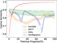
(a) Mean of distribution on credit

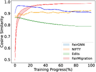
(b) Mean of distribution on bail

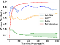
(c) Mean of distribution on income

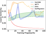
(d) Std of distribution on credit

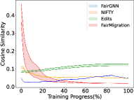
(e) Std of distribution on bail

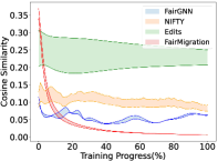
(f) Std of distribution on income

Figure 3. Visualization of group migration. The bold lines with the same color indicate the mean(std) of two group similarity distributions from the same method, respectively. The shaded areas indicate the group similarity distribution difference. The wider the shaded area on the y-axis, the larger similarity difference between groups

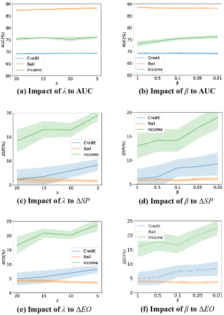
Figure 4. Visualization of hyperparameter $\lambda$ and $\beta$

5. Experiment

In this section, a series of experiments are conducted to demonstrate the effectiveness of our proposed model.

5.1. Datasets

We conduct experiments on three different real-world datasets credit, bail, and income. The statistics information of the the datasets is demonstrated in Table 2. The detailed introductions of these three datasets are as follows:

• Credit (Yeh and Lien, 2009): credit graph is built on 30, 000 credit card users. A node represents a user and the probability of generating an edge between two nodes depends on the similarity of their payment features. The label of credit is whether or not the user will default on credit card payments next month. The sensitive attribute is age.

• Bail (Jordan and Freiburger, 2015): bail (also known as recidivism) graph is built on 18, 876 defendants released on bail at the U.S. state courts from 1990 to 2009. A node represents a defendant and the probability of generating an edge between two nodes is determined by the similarity of their past criminal records and demographics. The label of bail is whether or not the defendant with bail. The sensitive attribute is race (white or not).

• Income: income graph is built on 14,821 individuals sampled from the Adult dataset (Dua and Graff, [n. d.]). A node represents a person. Take the similarity of a pair of nodes as the probability of establishing an edge between them. The label of income is whether or not the person earns more than 50K dollars. The sensitive attribute is race.

5.2. Baseline

In order to verify the effectiveness of FairMigration, three state-of-the-art GNN-based methods nifty, fairGNN, and EDITS are chosen for comparison. A brief introduction of these methods are following:

• Nifty (Agarwal et al., 2021). Nifty promotes the fairness by the counterfactual perturbation based siamese network and uses Lipschitz continuous function to normalize the layer weights.

• fairGNN (Dai and Wang, 2021). fairGNN is a adversarial training based method. It trains a sensitive attributes predictor to retrieve the sensitive attributes from the node embeddings while trains the GNN to reduce the information of the sensitive attributes in the node embeddings. We set al.l the sensitive attributes available for comparision.

• EDITS (Dong et al., 2022). EDITS transforms the attributes and regenerates the adjacency matrix for lowering the Wasserstein distance of attributes and topology between different demographic groups.

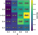
(a) Impact to AUC on credit

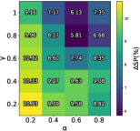
(b) Impact to $\Delta SP$ on credit

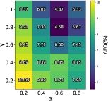
(c) Impact to $\Delta EO$ on credit

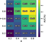
(d) Impact to AUC on bail

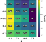
(e) Impact to $\Delta SP$ on bail

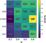
(f) Impact to $\Delta EO$ on bail

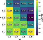
(g) Impact to AUC on income

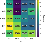
(h) Impact to $\Delta SP$ on income

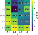
(i) Impact to $\Delta EO$ on income

Figure 5. Visualization of hyperparameter $\alpha$ and $\gamma$ of GCN

5.3. Evaluation Metrics

We use AUC-ROC to evaluate the performance of node classification. In addition, we use statistical parity($\Delta SP$, also known as demographic parity) and equal opportunity($\Delta EO$) to evaluate the fairness. The definition of $\Delta SP$ and $\Delta EO$ can be written as:

(22) $$\Delta SP=|P(\hat{y}=1|s=0)-P(\hat{y}=1|s=1)|$$

(23) $$\Delta EO=|P(\hat{y}=1|y=1,s=0)-P(\hat{y}=1|y=1,s=1)|$$

5.4. Implementation

The experiments are conducted on a server with Intel(R) Core(TM) i9-10980XE CPU @ 3.00GHz, NVIDIA 3090ti, Ubuntu 20.04 LTS, CUDA 11.3, python3.8, PyTorch 1.12.1, and PyTorch Geometric. Three popular GNNs, GCN, JK, and APPNP are adopted to be the backbone. The parameters range of experiments are following:

• FairGNN: $\alpha=4,\beta\in\{10,100,1000\}$.

• Nifty: $\lambda=0.5$.

• Edits: default $u_{1}$ to $u_{4}$. Threshold = 0.02 for credit, 0.015 for bail, 0.1 for income.

• FairMigration: $\lambda\in\{5,10,15,20\}$, $\beta\in\{0.01,0.05,0.1,0.5,1\}$, $\alpha\in\{0.2,0.4,0.6,0.8\}$, $\gamma\in\{0.2,0.4,0.6,0.8,1\}$

We run all experiments 10 times for preventing accidents as much as possible.

5.5. Experiment Results

In this subsection, we compare the node classification performance and fairness of FairMigration with the state-of-the-art models on three different GNNs. The comparison results of AUC-ROC, $\Delta SP$, and $\Delta EO$ are displayed in Table 3. The observations of the comparison can be summarized as:

• On different GNN backbones, FairMigration achieves competitive fairness with all baselines while the performance of node classification is comparable. It reveals the advances of FairMigration compared with other baselines.

• All baselines show varying degrees of unstable performance that sometimes perform well in fairness but badly in node classification, or on the contrary. For example, nifty shows poor performance in node classification in bail. FairMigration avoids this unstable situation, achieving higher unity of performance and fairness.

5.6. Ablation study

In order to fully understand the contribution of each component of FairMigration, we conduct ablation studies, and the results are shown in Table 4. Four variants of FairMigration removing one component are defined. The wo_mig denotes the variant removing the group migration. The wo_adv denotes the variant removing the adversarial training. The wo_ssf denotes the variant removing the personalized self-supervised learning. The wo_wei denotes the variant removing the reweight. Removing group migration or personalized self-supervised learning would result in the most significant deterioration in fairness and little changes in node classification. The combination of group migration and personalized self-supervised learning is a powerful technique to train fair GNNs. If Removing the adversarial training, FairMigration suffers from a fairness drop in most cases but enjoys fairness promotion in some cases. Adversarial training is an unstable strategy. Removing the reweight, FairMigration produces slightly biased results. The reweight technique can be a supplement to train fair GNNs.

5.7. Visualization of group migration

In this section, we take GCN as the backbone as an example, and visualize the group migration of baselines and FairMigration during the supervised learning stage. The change curve of mean and standard deviation of group similarity distribution is demonstrated in Figure 3. There are the following observations:

• The in-processing methods, Nifty, FairGNN, and FairMigration gradually eliminate the similarity distribution gap between groups during training. The pre-posting method Edits is still unable to completely get rid of the static biased information even though the data is preprocessed.

• Nifty and FairGNN show a certain degree of oscillation during training and they might not obtain a GNN fair enough with reasonable utility in some cases.

• FairMigration commendably bridges the differences between the two groups in all listed cases, demonstrating a remarkable ability to train fair GNNs.

5.8. Parameter Sensitivity

In order to investigate the impact of hyperparameters, $\lambda$, $\beta$, $\alpha$ and $\gamma$, we conducted experiments about parameter sensitivity, whose results are displayed in Figure 4 and Figure 5. The observations can be summarized as follows:

• $\lambda$ is the weight of group migration constraints in supervised learning. It almost doesn’t impact node classification but influences fairness a lot. GCN achieves the highest fairness in credit, bail, and income when $\lambda=20$, $\lambda=5$, and $\lambda=20$, respectively.

• $\beta$ is the weight of adversarial training in supervised learning. $\beta$ plays a little role in node classification in credit and bail but disturbs the node classification in income. The high value of $\beta$ would upgrade fairness in credit and income, but increase little biases in bail. FairMigration with GCN achieves the highest fairness in credit, bail, and income when $\beta=1$, $\beta=0.1$, and $\beta=1$, respectively.

• $\alpha$ is the trade-off between contrastive learning and reconstruction. $\gamma$ is the weight of personalized self-supervised learning. It is a hard task to find a combination of $\alpha$ and $\gamma$ that obtain the best node classification performance and fairness simultaneously. But, the optimal combination of $\alpha$ and $\gamma$ in node classification is very closed to that in fairness.

6. conclusion and the future direction

In this paper, we explore a novel aspect of fairness, breaking the limitation of static sensitive attributes for training fair GNN. We propose an innovative framework FairMigration, reallocating the demographic groups dynamically instead of maintaining the demographic group division following the raw sensitive attributes. FairMigration preliminarily optimizes the encoder mainly for fairness by personalized self-supervised learning and dynamically migrates the groups. After that, the migrated groups and the adversarial training are adopted to constrain supervised learning. The extensive experiments exhibit the effectiveness of FairMigration in both downstream tasks and fairness. The group migration strategy is an interesting direction. FairMigration adopts a simple flip strategy. However, the optimal number of migrated groups may not be the same as the raw groups. Therefore, we will study the optimal migrated group division and extend it to multi-value sensitive attributes.

References

- (1)
- Agarwal et al. (2021) Chirag Agarwal, Himabindu Lakkaraju, and Marinka Zitnik. 2021. Towards a unified framework for fair and stable graph representation learning. In Uncertainty in Artificial Intelligence. PMLR, 2114–2124.
- Beutel et al. (2017) Alex Beutel, Jilin Chen, Zhe Zhao, and Ed H. Chi. 2017. Data Decisions and Theoretical Implications when Adversarially Learning Fair Representations. CoRR abs/1707.00075 (2017). arXiv:1707.00075 http://arxiv.org/abs/1707.00075
- Cai et al. (2021) Lei Cai, Jundong Li, Jie Wang, and Shuiwang Ji. 2021. Line graph neural networks for link prediction. IEEE Transactions on Pattern Analysis and Machine Intelligence 44, 9 (2021), 5103–5113.
- Chai and Wang (2022) Junyi Chai and Xiaoqian Wang. 2022. Fairness with adaptive weights. In International Conference on Machine Learning. PMLR, 2853–2866.
- Choudhary et al. (2022) Manvi Choudhary, Charlotte Laclau, and Christine Largeron. 2022. A survey on fairness for machine learning on graphs. arXiv preprint arXiv:2205.05396 (2022).
- Creager et al. (2019) Elliot Creager, David Madras, Jörn-Henrik Jacobsen, Marissa Weis, Kevin Swersky, Toniann Pitassi, and Richard Zemel. 2019. Flexibly fair representation learning by disentanglement. In International conference on machine learning. PMLR, 1436–1445.
- Dai and Wang (2021) Enyan Dai and Suhang Wang. 2021. Say no to the discrimination: Learning fair graph neural networks with limited sensitive attribute information. In Proceedings of the 14th ACM International Conference on Web Search and Data Mining. 680–688.
- Dong et al. (2021) Yushun Dong, Kaize Ding, Brian Jalaian, Shuiwang Ji, and Jundong Li. 2021. Adagnn: Graph neural networks with adaptive frequency response filter. In Proceedings of the 30th ACM International Conference on Information & Knowledge Management. 392–401.
- Dong et al. (2022) Yushun Dong, Ninghao Liu, Brian Jalaian, and Jundong Li. 2022. Edits: Modeling and mitigating data bias for graph neural networks. In Proceedings of the ACM Web Conference 2022. 1259–1269.
- Dua and Graff ([n. d.]) Dheeru Dua and Casey Graff. [n. d.]. UCI Machine Learning Repository. http://archive.ics.uci.edu/ml/index.php.
- Dwork et al. (2012) Cynthia Dwork, Moritz Hardt, Toniann Pitassi, Omer Reingold, and Richard Zemel. 2012. Fairness through awareness. In Proceedings of the 3rd innovations in theoretical computer science conference. 214–226.
- Garg et al. (2019) Sahaj Garg, Vincent Perot, Nicole Limtiaco, Ankur Taly, Ed H Chi, and Alex Beutel. 2019. Counterfactual fairness in text classification through robustness. In Proceedings of the 2019 AAAI/ACM Conference on AI, Ethics, and Society. 219–226.
- Gasteiger et al. (2018) Johannes Gasteiger, Aleksandar Bojchevski, and Stephan Günnemann. 2018. Predict then propagate: Graph neural networks meet personalized pagerank. arXiv preprint arXiv:1810.05997 (2018).
- Gwadabe and Liu (2022) Tajuddeen Rabiu Gwadabe and Ying Liu. 2022. Improving graph neural network for session-based recommendation system via non-sequential interactions. Neurocomputing 468 (2022), 111–122.
- Hamilton et al. (2017) William L. Hamilton, Rex Ying, and Jure Leskovec. 2017. Inductive Representation Learning on Large Graphs. CoRR abs/1706.02216 (2017). arXiv:1706.02216 http://arxiv.org/abs/1706.02216
- Jalal et al. (2021) Ajil Jalal, Sushrut Karmalkar, Jessica Hoffmann, Alex Dimakis, and Eric Price. 2021. Fairness for image generation with uncertain sensitive attributes. In International Conference on Machine Learning. PMLR, 4721–4732.
- Jiang et al. (2022) Zhimeng Jiang, Xiaotian Han, Chao Fan, Zirui Liu, Na Zou, Ali Mostafavi, and Xia Hu. 2022. Fmp: Toward fair graph message passing against topology bias. arXiv preprint arXiv:2202.04187 (2022).
- Jin et al. (2022) Jiayin Jin, Zeru Zhang, Yang Zhou, and Lingfei Wu. 2022. Input-agnostic certified group fairness via gaussian parameter smoothing. In International Conference on Machine Learning. PMLR, 10340–10361.
- Jordan and Freiburger (2015) Kareem L Jordan and Tina L Freiburger. 2015. The effect of race/ethnicity on sentencing: Examining sentence type, jail length, and prison length. Journal of Ethnicity in Criminal Justice 13, 3 (2015), 179–196.
- Kipf and Welling (2016) Thomas N Kipf and Max Welling. 2016. Semi-supervised classification with graph convolutional networks. arXiv preprint arXiv:1609.02907 (2016).
- Köse and Shen (2021) Öykü Deniz Köse and Yanning Shen. 2021. Fairness-aware node representation learning. arXiv preprint arXiv:2106.05391 (2021).
- Kose and Shen (2022) O Deniz Kose and Yanning Shen. 2022. Fair node representation learning via adaptive data augmentation. arXiv preprint arXiv:2201.08549 (2022).
- Lahoti et al. (2019) Preethi Lahoti, Krishna P Gummadi, and Gerhard Weikum. 2019. Operationalizing individual fairness with pairwise fair representations. arXiv preprint arXiv:1907.01439 (2019).
- Lohia et al. (2019) Pranay K Lohia, Karthikeyan Natesan Ramamurthy, Manish Bhide, Diptikalyan Saha, Kush R Varshney, and Ruchir Puri. 2019. Bias mitigation post-processing for individual and group fairness. In Icassp 2019-2019 ieee international conference on acoustics, speech and signal processing (icassp). IEEE, 2847–2851.
- Long et al. (2022) Yahui Long, Min Wu, Yong Liu, Yuan Fang, Chee Keong Kwoh, Jinmiao Chen, Jiawei Luo, and Xiaoli Li. 2022. Pre-training graph neural networks for link prediction in biomedical networks. Bioinformatics 38, 8 (2022), 2254–2262.
- Ma et al. (2022) Jing Ma, Ruocheng Guo, Mengting Wan, Longqi Yang, Aidong Zhang, and Jundong Li. 2022. Learning fair node representations with graph counterfactual fairness. In Proceedings of the Fifteenth ACM International Conference on Web Search and Data Mining. 695–703.
- Mehrabi et al. (2021) Ninareh Mehrabi, Fred Morstatter, Nripsuta Saxena, Kristina Lerman, and Aram Galstyan. 2021. A survey on bias and fairness in machine learning. ACM Computing Surveys (CSUR) 54, 6 (2021), 1–35.
- Mehrotra and Celis (2021) Anay Mehrotra and L Elisa Celis. 2021. Mitigating bias in set selection with noisy protected attributes. In Proceedings of the 2021 ACM Conference on Fairness, Accountability, and Transparency. 237–248.
- Mishler et al. (2021) Alan Mishler, Edward H Kennedy, and Alexandra Chouldechova. 2021. Fairness in risk assessment instruments: Post-processing to achieve counterfactual equalized odds. In Proceedings of the 2021 ACM Conference on Fairness, Accountability, and Transparency. 386–400.
- Putzel and Lee (2022) Preston Putzel and Scott Lee. 2022. Blackbox post-processing for multiclass fairness. arXiv preprint arXiv:2201.04461 (2022).
- Qiu et al. (2022) Chenyang Qiu, Zhaoci Huang, Wenzhe Xu, and Huijia Li. 2022. VGAER: graph neural network reconstruction based community detection. arXiv preprint arXiv:2201.04066 (2022).
- Shchur and Günnemann (2019) Oleksandr Shchur and Stephan Günnemann. 2019. Overlapping community detection with graph neural networks. arXiv preprint arXiv:1909.12201 (2019).
- Song et al. (2022) Weihao Song, Yushun Dong, Ninghao Liu, and Jundong Li. 2022. Guide: Group equality informed individual fairness in graph neural networks. In Proceedings of the 28th ACM SIGKDD Conference on Knowledge Discovery and Data Mining. 1625–1634.
- Spinelli et al. (2021) Indro Spinelli, Simone Scardapane, Amir Hussain, and Aurelio Uncini. 2021. Biased Edge Dropout for Enhancing Fairness in Graph Representation Learning. CoRR abs/2104.14210 (2021). arXiv:2104.14210 https://arxiv.org/abs/2104.14210
- Sun et al. (2021) Jianyong Sun, Wei Zheng, Qingfu Zhang, and Zongben Xu. 2021. Graph neural network encoding for community detection in attribute networks. IEEE Transactions on Cybernetics 52, 8 (2021), 7791–7804.
- Ustun et al. (2019) Berk Ustun, Yang Liu, and David Parkes. 2019. Fairness without harm: Decoupled classifiers with preference guarantees. In International Conference on Machine Learning. PMLR, 6373–6382.
- Veličković et al. (2017) Petar Veličković, Guillem Cucurull, Arantxa Casanova, Adriana Romero, Pietro Lio, and Yoshua Bengio. 2017. Graph attention networks. arXiv preprint arXiv:1710.10903 (2017).
- Wang et al. (2022a) Jiayin Wang, Weizhi Ma, Jiayu Li, Hongyu Lu, Min Zhang, Biao Li, Yiqun Liu, Peng Jiang, and Shaoping Ma. 2022a. Make Fairness More Fair: Fair Item Utility Estimation and Exposure Re-Distribution. In Proceedings of the 28th ACM SIGKDD Conference on Knowledge Discovery and Data Mining. 1868–1877.
- Wang et al. (2023) Rui Wang, Pengyu Cheng, and Ricardo Henao. 2023. Toward Fairness in Text Generation via Mutual Information Minimization based on Importance Sampling. In International Conference on Artificial Intelligence and Statistics. PMLR, 4473–4485.
- Wang et al. (2022b) Ruijia Wang, Xiao Wang, Chuan Shi, and Le Song. 2022b. Uncovering the Structural Fairness in Graph Contrastive Learning. arXiv preprint arXiv:2210.03011 (2022).
- Wang et al. (2022c) Yu Wang, Yuying Zhao, Yushun Dong, Huiyuan Chen, Jundong Li, and Tyler Derr. 2022c. Improving fairness in graph neural networks via mitigating sensitive attribute leakage. In Proceedings of the 28th ACM SIGKDD Conference on Knowledge Discovery and Data Mining. 1938–1948.
- Xu et al. (2018a) Keyulu Xu, Weihua Hu, Jure Leskovec, and Stefanie Jegelka. 2018a. How powerful are graph neural networks? arXiv preprint arXiv:1810.00826 (2018).
- Xu et al. (2018b) Keyulu Xu, Chengtao Li, Yonglong Tian, Tomohiro Sonobe, Ken-ichi Kawarabayashi, and Stefanie Jegelka. 2018b. Representation Learning on Graphs with Jumping Knowledge Networks. CoRR abs/1806.03536 (2018). arXiv:1806.03536 http://arxiv.org/abs/1806.03536
- Yeh and Lien (2009) I-Cheng Yeh and Che-hui Lien. 2009. The comparisons of data mining techniques for the predictive accuracy of probability of default of credit card clients. Expert systems with applications 36, 2 (2009), 2473–2480.
- Yin et al. (2019) Ruiping Yin, Kan Li, Guangquan Zhang, and Jie Lu. 2019. A deeper graph neural network for recommender systems. Knowledge-Based Systems 185 (2019), 105020.
- Yu et al. (2021) Jun Yu, Xinlong Hao, Zeyu Cui, Peng He, and Tongliang Liu. 2021. Boosting fairness for masked face recognition. In Proceedings of the IEEE/CVF International Conference on Computer Vision. 1531–1540.
- Zhang and Chen (2018) Muhan Zhang and Yixin Chen. 2018. Link prediction based on graph neural networks. Advances in neural information processing systems 31 (2018).
- Zhao et al. (2022) Tianxiang Zhao, Enyan Dai, Kai Shu, and Suhang Wang. 2022. Towards fair classifiers without sensitive attributes: Exploring biases in related features. In Proceedings of the Fifteenth ACM International Conference on Web Search and Data Mining. 1433–1442.