Two-step inertial Bregman alternating structure-adapted proximal gradient descent algorithm for nonconvex and nonsmooth problems

Abstract. In this paper, we propose accelerated alternating structure-adapted proximal gradient descent method for a class of nonconvex and nonsmooth nonseparable problems. The proposed algorithm is a monotone method which combines two-step inertial extrapolation and Bregman distance. Under some assumptions, we prove that every cluster point of the sequence generated by the proposed algorithm is a critical point. Furthermore, with the help of Kurdyka–Łojasiewicz property, we establish the convergence of the whole sequence generated by proposed algorithm. In order to make the algorithm more effective and flexible, we also use some strategies to update the extrapolation parameter and solve the problems with unknown Lipschitz constant. Moreover, we report some preliminary numerical results on involving nonconvex quadratic programming and sparse logistic regression to show the feasibility and effectiveness of the proposed methods.

Key words: Accelerated methods; Nonconvex and nonsmooth nonseparable optimization; Extrapolation; Bregman distance; Kurdyka–Łojasiewicz property.

1 Introduction

In this paper, we will consider to solve the following nonconvex and nonsmooth nonseparable optimization problem:

$$\min_{x\in\mathbb{R}^{n},y\in\mathbb{R}^{m}}L(x,y)=f(x)+Q(x,y)+g(y),$$ (1.1)

where $f:\mathbb{R}^{n}\to\mathbb{R}$, $g:\mathbb{R}^{m}\to\mathbb{R}$ are continuously differentiable, $Q:\mathbb{R}^{n}\times\mathbb{R}^{m}\to\mathbb{R}\cup\left\{\infty\right\}$ is a proper, lower semicontinuous function. Note that here and throughout the paper, no convexity is assumed on the objective function. Problem (1.1) is used in many application scenarios, such as signal recovery [1, 2, 3], nonnegative matrix facorization [4, 5], quadratic fractional programming [6, 7], compressed sensing [8, 9], sparse logistic regression [7] and so on.

The natural method to solve problem (1.1) is the alternating minimization (AM) method (also called block coordinate descent (BCD) method), which, from a given initial point $\left(x_{0},y_{0}\right)\in\mathbb{R}^{n}\times\mathbb{R}^{m}$, generates the iterative sequence $\left\{\left(x_{k},y_{k}\right)\right\}$ via the scheme:

$$\begin{cases}x_{k+1}\in\arg\min_{x\in\mathbb{R}^{n}}\{L(x,y_{k})\},\\ y_{k+1}\in\arg\min_{y\in\mathbb{R}^{m}}\{L(x_{k+1},y)\}.\\ \end{cases}$$ (1.2)

If $L(x,y)$ is convex and continuously differentiable, and it is strict convex of one argument while the other is fixed, then the sequence converges to a critical point [10, 11].

To relax the requirements of AM method and remove the strict convexity assumption, Auslender [12] introduced proximal terms to (1.2) for convex function $L$:

$$\begin{cases}x_{k+1}\in\arg\min_{x\in\mathbb{R}^{n}}\{L(x,y_{k})+\frac{1}{2\lambda_{k}}\|x-x_{k}\|^{2}_{2}\},\\ y_{k+1}\in\arg\min_{y\in\mathbb{R}^{m}}\{L(x_{k+1},y)+\frac{1}{2\mu_{k}}\|y-y_{k}\|^{2}_{2}\},\\ \end{cases}$$ (1.3)

where $\{\lambda_{k}\}_{k\in\mathbb{N}}$ and $\{\mu_{k}\}_{k\in\mathbb{N}}$ are positive sequences. The above proximal point method, which is called proximal alternating minimization (PAM) algorithm, was further extended to nonconvex nonsmooth functions. Such as, in [13], Attouch et al. applied (1.3) to solve nonconvex problem (1.1) and proved the sequence generated by the proximal alternating minimization algorithm (1.3) converges to a critical point. More convergence analysis of the proximal point method can be found in [14, 15].

Because the proximal alternating minimization algorithm requires an exact solution at each iteration step, the subproblems are very expensive if the minimizers of subproblems are not given in a closed form. The linearization technique is one of the effective methods to overcome the absence of an analytic solution to the subproblem. Bolte et al. [16] proposed the following proximal alternating linearized minimization (PALM) algorithm under the condition that the coupling term $Q(x,y)$ is continuously differentiable:

$$\begin{cases}x_{k+1}\in\arg\min_{x\in\mathbb{R}^{n}}\{f(x)+\langle x,\nabla_{x}Q(x_{k},y_{k})\rangle+\frac{1}{2\lambda_{k}}\|x-x_{k}\|^{2}_{2}\},\\ y_{k+1}\in\arg\min_{y\in\mathbb{R}^{m}}\{g(y)+\langle y,\nabla_{y}Q(x_{k+1},y_{k})\rangle+\frac{1}{2\mu_{k}}\|y-y_{k}\|^{2}_{2}\}.\\ \end{cases}$$ (1.4)

The step size $\lambda_{k}$ and $\mu_{k}$ are limited to

$$\lambda_{k}\in(0,({\rm Lip}(\bigtriangledown_{x}Q(\cdot,y_{k})))^{-1}),\mu_{k}\in(0,({\rm Lip}(\bigtriangledown_{y}Q(x_{k+1},\cdot)))^{-1}),$$

where “Lip” denotes the Lipschitz constant of the function in parentheses. In this way, the solution of some subproblems may be expressed by a closed-form or can be easily calculated. The global convergence result was established if $L(x,y)$ satisfied the Kurdyka–Łojasiewicz property.

When $f$ and $g$ are continuously differentiable, a natural idea is to linearize $f$ and $g$. Nikolova et al. [17] proposed the corresponding algorithm, called alternating structure-adapted proximal gradient descent (ASAP) algorithm with the following scheme:

$$\begin{cases}x_{k+1}\in\arg\underset{x\in\mathbb{R}^{n}}{\min}\{Q(x,y_{k})+\langle x,\nabla f(x_{k})\rangle+\frac{1}{2\sigma}\|x-x_{k}\|^{2}_{2}\},\\ y_{k+1}\in\arg\underset{y\in\mathbb{R}^{m}}{\min}\{Q(x_{k+1},y)+\langle y,\nabla g(y_{k})\rangle+\frac{1}{2\tau}\|y-y_{k}\|^{2}_{2}\},\\ \end{cases}$$ (1.5)

where $\sigma\in(0,({\rm Lip}(\bigtriangledown f))^{-1}),\tau\in(0,({\rm Lip}(\bigtriangledown g))^{-1})$. With the help of Kurdyka–Łojasiewicz property they establish the convergence of the whole sequence generated by (1.5).

The inertial extrapolation technique has been widely used to accelerate the iterative algorithms for convex and nonconvex optimizations, since the cost of each iteration stays basically unchanged [18, 19]. The inertial scheme, starting from the so-called heavy ball method of Polyak [20], was recently proved to be very efficient in accelerating numerical methods, especially the first-order methods. Alvarez et al. [21] applied the inertial strategy to the proximal point method and proved that it could improve the rate of convergence. The main feature of the idea is that the new iteration use the previous two or more iterations.

Based on (1.4), Pock and Sabach [22] proposed the following inertial proximal alternating linearized minimization (iPALM) algorithm:

$$\begin{cases}u_{1k}=x_{k}+\alpha_{1k}(x_{k}-x_{k-1}),v_{1k}=x_{k}+\beta_{1k}(x_{k}-x_{k-1}),\\ x_{k+1}\in\arg\min_{x\in\mathbb{R}^{n}}\{f(x)+\langle x,\nabla_{x}Q(v_{1k},y_{k})\rangle+\frac{1}{2\lambda_{k}}\|x-u_{1k}\|^{2}_{2}\},\\ u_{2k}=y_{k}+\alpha_{2k}(y_{k}-y_{k-1}),v_{2k}=y_{k}+\beta_{2k}(y_{k}-y_{k-1}),\\ y_{k+1}\in\arg\min_{y\in\mathbb{R}^{m}}\{g(y)+\langle y,\nabla_{y}Q(x_{k+1},v_{2k})\rangle+\frac{1}{2\mu_{k}}\|y-u_{2k}\|^{2}_{2}\},\\ \end{cases}$$ (1.6)

where $\alpha_{1k},\alpha_{2k},\beta_{1k},\beta_{2k}\in\left[0,1\right]$. They proved that the generated sequence globally converges to critical point of the objective function under the condition of the Kurdyka–Łojasiewicz property. When $\alpha_{1k}\equiv\alpha_{2k}\equiv\beta_{1k}\equiv\beta_{2k}\equiv 0$, iPALM reduces to PALM. Then Cai et al. [23] presented a Gauss–Seidel type inertial proximal alternating linearized minimization (GiPALM) algorithm for solving problem (1.1):

$$\begin{cases}x_{k+1}\in\arg\min_{x\in\mathbb{R}^{n}}\{f(x)+\langle x,\nabla_{x}Q(\tilde{x}_{k},\tilde{y}_{k})\rangle+\frac{1}{2\lambda_{k}}\|x-\tilde{x}_{k}\|^{2}_{2}\},\\ \tilde{x}_{k+1}=x_{k+1}+\alpha(x_{k+1}-\tilde{x}_{k}),\alpha\in[0,1),\\ y_{k+1}\in\arg\min_{y\in\mathbb{R}^{m}}\{g(y)+\langle y,\nabla_{y}Q(\tilde{x}_{k+1},\tilde{y}_{k})\rangle+\frac{1}{2\mu_{k}}\|y-\tilde{y}_{k}\|^{2}_{2}\},\\ \tilde{y}_{k+1}=y_{k+1}+\beta(y_{k+1}-\tilde{y}_{k}),\beta\in[0,1).\end{cases}$$ (1.7)

By using inertial extrapolation technique, Xu et al. [7] proposed the following accelerated alternating structure-adapted proximal gradient descent (aASAP) algorithm:

$$\begin{cases}x_{k+1}\in\arg\min_{x\in\mathbb{R}^{n}}\{Q(x,\hat{y}_{k})+\langle\nabla f(\hat{x}_{k}),x\rangle+\frac{1}{2\sigma}\|x-\hat{x}_{k}\|^{2}_{2}\},\\ y_{k+1}\in\arg\min_{y\in\mathbb{R}^{m}}\{Q(x_{k+1},y)+\langle\nabla g(\hat{y}_{k}),y\rangle+\frac{1}{2\tau}\|y-\hat{y}_{k}\|^{2}_{2}\},\\ u_{k+1}=x_{k+1}+\beta_{k}(x_{k+1}-x_{k}),v_{k+1}=y_{k+1}+\beta_{k}(y_{k+1}-y_{k}),\\ {\rm if}\ L(u_{k+1},v_{k+1})\leq L(x_{k+1},y_{k+1}),\ {\rm then}\ \hat{x}_{k+1}=u_{k+1},\hat{y}_{k+1}=v_{k+1},\\ {\rm else}\ \hat{x}_{k+1}=x_{k+1},\hat{y}_{k+1}=y_{k+1}.\end{cases}$$ (1.8)

Compared with the traditional extrapolation algorithm, the main difference is to ensure that the algorithm is a monotone method in terms of objective function value, while general extrapolation algorithms may be nonmonotonic.

Bregman distance is a useful substitute for a distance, obtained from the various choices of functions. The applications of Bregman distance instead of the norm gives us alternative ways for more flexibility in the selection of regularization. Choosing appropriate Bregeman distances can obtain colsed form of solution for solving some subproblem. Bregman distance regularization is also an effective way to improve the numerical results of the algorithm. In [24], the authors constructed the following two-step inertial Bregman alternating minimization algorithm using the information of the previous three iterates:

$$\begin{cases}x_{k+1}\in\arg\min_{x\in\mathbb{R}^{n}}\{L(x,y_{k})+D_{\phi_{1}}(x,x_{k})+\alpha_{1k}\langle x,x_{k-1}-x_{k}\rangle+\alpha_{2k}\langle x,x_{k-2}-x_{k-1}\rangle\},\\ y_{k+1}\in\arg\min_{y\in\mathbb{R}^{m}}\{L(x_{k+1},y)+D_{\phi_{2}}(y,y_{k})+\beta_{1k}\langle y,y_{k-1}-y_{k}\rangle+\beta_{2k}\langle y,y_{k-2}-y_{k-1}\},\end{cases}$$ (1.9)

where $D_{\phi_{i}}(i=1,2)$ denotes the Bregman distance with respect to $\phi_{i}(i=1,2)$, respectively. The convergence is obtained provided an appropriate regularization of the objective function satisfies the Kurdyka–Łojasiewicz inequality. Based on alternating minimization algorithm, Zhao et al. [25] proposed the following inertial alternating minimization with Bregman distance (BIAM) algorithm:

$$\begin{cases}x_{k+1}\in\arg\min_{x\in\mathbb{R}^{n}}\{f(x)+Q(x,\hat{y}_{k})+\lambda_{k}D_{\phi_{1}}(x,\hat{x}_{k})\},\\ \hat{x}_{k+1}=x_{k+1}+\alpha(x_{k+1}-\hat{x}_{k}),\alpha\in[0,1),\\ y_{k+1}\in\arg\min_{y\in\mathbb{R}^{m}}\{g(y)+Q(\hat{x}_{k+1},y)+\mu_{k}D_{\phi_{2}}(y,\hat{y}_{k})\},\\ \hat{y}_{k+1}=y_{k+1}+\beta(y_{k+1}-\hat{y}_{k}),\beta\in[0,1).\end{cases}$$ (1.10)

Suppose that the benefit function satisfies the Kurdyka–Łojasiewicz property and the parameters are selected appropriately, they proved the convergence of BIAM algorithm.

In this paper, based on the alternating structure-adapted proximal gradient methods, we combine inertial extrapolation technique and Bregman distance to construct two-step inertial Bregman alternating structure-adapted proximal gradient descent algorithm. And in order to make the proposed algorithm more effective and flexible, we also use some strategies to update the extrapolation parameter and solve the problems with unknown Lipschitz constant. Under some assumptions about the penalty parameter and objective function, the convergence of the proposed algorithm is obtained based on the Kurdyka–Łojasiewicz property. Moreover, we report some preliminary numerical results on involving quadratic programming and logistic regression problem to show the feasibility and effectiveness of the proposed method.

The article is organized as follows. In Section 2, we recall some concepts and important lemmas which will be used in the proof of main results. In Section 3, we present the Two-step inertial Bregman alternating structure-adapted proximal gradient algorithm and show its convergence. Finally, in Section 4, the preliminary numerical examples on nonconvex quadratic programming and sparse logistic regression problem are provided to illustrate the behavior of the proposed algorithm.

2 Preliminaries

Consider the Euclidean vector space $\mathbb{R}^{d}$ of dimension $d\geq 1$, the standard inner product and the induced norm on $\mathbb{R}^{d}$ are denoted by $\langle\cdot,\cdot\rangle$ and $\|\cdot\|_{2}$, respectively. We use $\omega(x_{k})=\{x:\exists x_{k_{j}}\rightarrow x\}$ to stand for the limit set of $\{x_{k}\}_{k\in\mathbb{N}}$.

The domain of $f$ are defined by dom$f:=\{x\in\mathbb{R}^{d}:f(x)<+\infty\}$. We say that $f$ is proper if dom$f\neq\emptyset$, and $f$ is called lower semicontinuous at $x$ if $f(x)\leq\lim\inf_{k\to\infty}f(x_{k})$ for every sequence $\left\{x_{k}\right\}$ converging to $x$. If $f$ is lower semicontinuous in its domain, we say $f$ is a lower semicontinuous function. If dom$f$ is closed and $f$ is lower semicontinuous over dom$f$ , then $f$ is a closed function. Further we recall some generalized subdifferential notions and the basic properties which are needed in this paper.

2.1 Subdifferentials

Definition 2.1.

(Subdifferentials) Let $f:\mathbb{R}^{d}\rightarrow(-\infty,+\infty]$ be a proper and lower semicontinuous function.

(i)For $x\in$ dom$f$, the Fréchet subdifferential of $f$ at $x$, written $\hat{\partial}f(x)$, is the set of vectors $v\in\mathbb{R}^{d}$ which satisfy

$$\liminf_{y\rightarrow x}\frac{1}{\|x-y\|_{2}}[f(y)-f(x)-\langle v,y-x\rangle]\geq 0.$$

(ii)If $x\not\in$ dom$f$, then $\hat{\partial}f(x)=\emptyset$. The limiting-subdifferential [26], or simply the subdifferential for short, of $f$ at $x\in$ dom$f$, written $\partial f(x)$, is defined as follows:

$$\partial f(x):=\{v\in\mathbb{R}^{d}:\exists x_{k}\rightarrow x,f(x_{k})\rightarrow f(x),v_{k}\in\hat{\partial}f(x_{k}),v_{k}\rightarrow v\}.$$

Remark 2.1.

(a) The above definition implies that $\hat{\partial}f(x)\subseteq\partial f(x)$ for each $x\in\mathbb{R}^{d}$, where the first set is convex and closed while the second one is closed (see[27]).

(b) (Closedness of $\partial f$) Let $\{x_{k}\}_{k\in\mathbb{N}}$ and $\{v_{k}\}_{k\in\mathbb{N}}$ be sequences in $\mathbb{R}^{d}$ such that $v_{k}\in\partial f(x_{k})$ for all $k\in\mathbb{N}$. If $(x_{k},v_{k})\rightarrow(x,v)$ and $f(x_{k})\rightarrow f(x)$ as $k\rightarrow\infty$, then $v\in\partial f(x)$.

(c) If $f:\mathbb{R}^{d}\rightarrow(-\infty,+\infty]$ be a proper and lower semicontinuous and $h:\mathbb{R}^{d}\rightarrow\mathbb{R}$ is a continuously differentiable function, then $\partial(f+h)(x)=\partial f(x)+\nabla h(x)$ for all $x\in\mathbb{R}^{d}$.

In what follows, we will consider the problem of finding a critical point $(x^{\ast},y^{\ast})\in$dom$L$.

Lemma 2.1.

(Fermat’s rule[28]) Let $f:\mathbb{R}^{d}\rightarrow\mathbb{R}\cup\left\{+\infty\right\}$ be a proper lower semicontinuous function. If $f$ has a local minimum at $x^{\ast}$, then $0\in\partial f(x^{\ast})$.

We call $x^{\ast}$ is a critical point of $f$ if  $0\in\partial f(x^{\ast})$. The set of all critical points of $f$ denoted by crit$f$.

Lemma 2.2.

(Descent lemma[29]) Let $h:\mathbb{R}^{d}\rightarrow\mathbb{R}$ be a continuously differentiable function with gradient $\nabla h$ assumed $L_{h}$-Lipschitz continuous. Then

$$h\left(u\right)\leq h\left(v\right)+\left\langle u-v,\nabla h\left(v\right)\right\rangle+\frac{L_{h}}{2}{\left\|u-v\right\|^{2}_{2},\ \forall u,v\in\mathbb{R}^{d}.}$$ (2.1)

2.2 The Kurdyka–Łojasiewicz property

In this section, we recall the KŁ property, which plays a central role in the convergence analysis.

Definition 2.2.

(Kurdyka–Łojasiewicz property [13]) Let $f:\mathbb{R}^{d}\rightarrow(-\infty,+\infty]$ be a proper and lower semicontinuous function.

(i)The function $f:\mathbb{R}^{d}\rightarrow(-\infty,+\infty]$ is said to have the Kurdyka–Łojasiewicz (KŁ) property at $x^{\ast}\in$dom$f$ if there exist $\eta\in(0,+\infty]$, a neighborhood $U$ of $x^{\ast}$ and a continuous concave function $\varphi:[0,\eta)\rightarrow\mathbb{R}_{+}$ such that $\varphi(0)=0$, $\varphi$ is $C^{1}$ on $(0,\eta)$, for all $s\in(0,\eta)$ it is $\varphi^{\prime}(s)>0$ and for all $x$ in $U\cap[f(x^{\ast})<f<f(x^{\ast})+\eta]$ the Kurdyka–Łojasiewicz inequality holds,

$$\varphi^{\prime}(f(x)-f(x^{\ast})){\rm dist}(0,\partial f(x))\geq 1.$$

(ii)Proper lower semicontinuous functions which satisfy the Kurdyka–Łojasiewicz inequality at each point of its domain are called KŁ functions.

Lemma 2.3.

(Uniformized KŁ property[28]) Let $\Omega$ be a compact set and let $f:\mathbb{R}^{d}\rightarrow\mathbb{R}\cup\left\{+\infty\right\}$ be a proper and lower semicontinuous function. Assume that $f$ is constant on $\Omega$ and satisfies the KŁ property at each point of $\Omega$. Then, there exist $\varepsilon>0,\eta>0$ and $\varphi\in\Phi_{\eta}$ such that for all $x^{\ast}\in\Omega$ and for all $x\in\left\{x\in\mathbb{R}^{d}:{\rm dist}(x,\Omega)<\varepsilon\right\}\cap[f(x^{\ast})<f<f(x^{\ast})+\eta]$, one has

$$\varphi^{\prime}(f(x)-f(x^{\ast})){\rm dist}(0,\partial f(x))\geq 1.$$

There is a broad class of functions satisfy the KŁ property, such as strongly convex functions, real analytic functions, semi-algebraic functions [13], subanalytic functions [30], log-exp functions and so on.

2.3 Bregman distance

Definition 2.3.

A function $f$ is said convex if dom$f$ is a convex set and if, for all $x$, $y\in$dom$f$, $\alpha\in[0,1]$,

$$f(\alpha x+(1-\alpha)y)\leq\alpha f(x)+(1-\alpha)f(y).$$

$f$ is said $\theta$-strongly convex with $\theta>0$ if $f-\frac{\theta}{2}\|\cdot\|^{2}$ is convex, i.e.,

$$f(\alpha x+(1-\alpha)y)\leq\alpha f(x)+(1-\alpha)f(y)-\frac{1}{2}\theta\alpha(1-\alpha)\|x-y\|^{2}$$

for all $x$, $y\in$dom$f$ and $\alpha\in[0,1]$.

Suppose that the function $f$ is differentiable. Then $f$ is convex if and only if dom$f$ is a convex set and

$$f(x)\geq f(y)+\langle\nabla f(y),x-y\rangle$$

holds for all $x$, $y\in$dom$f$. Moreover, $f$ is $\theta$-strongly convex with $\theta>0$ if and only if

$$f(x)\geq f(y)+\langle\nabla f(y),x-y\rangle+\frac{\theta}{2}\|x-y\|^{2}$$

for all $x$, $y\in$dom$f$.

Definition 2.4.

Let $\phi:\mathbb{R}^{d}\rightarrow(-\infty,+\infty]$ be a convex and Gâteaux differentiable function. The function $D_{\phi}:$ dom$\phi\,\,\times$ intdom$\phi\rightarrow[0,+\infty)$, defined by

$$D_{\phi}(x,y)=\phi(x)-\phi(y)-\langle\nabla\phi(y),x-y\rangle,$$

is called the Bregman distance with respect to $\phi$.

From the above definition, it follows that

$$D_{\phi}(x,y)\geq\frac{\theta}{2}\|x-y\|^{2},$$ (2.2)

if $\phi$ is $\theta$-strongly convex.

3 Algorithm and convergence analysis

Assumption 3.1.

(i) $L:\mathbb{R}^{n}\times\mathbb{R}^{m}\to\mathbb{R}\cup\left\{\infty\right\}$ is lower bounded.

(ii) $f:\mathbb{R}^{n}\to\mathbb{R}$ and $g:\mathbb{R}^{m}\to\mathbb{R}$ are continuously differentiable and their gradients $\nabla f$ and $\nabla g$ are Lipschitz continuous with constants $L_{\nabla f}$, $L_{\nabla g}$ respectively.

(iii) $Q:\mathbb{R}^{n}\times\mathbb{R}^{m}\to\mathbb{R}\cup\left\{\infty\right\}$ is a proper, lower semicontinuous.

(iv) $\phi_{i}(i=1,2)$ is $\theta_{i}$-strongly convex differentiable function, $\theta_{1}>L_{\nabla f}$, $\theta_{2}>L_{\nabla g}$. And the gradient $\nabla\phi_{i}$ is $\eta_{i}$-Lipschitz continuous, i.e.,

$$\left\|\nabla{\phi_{1}}(x)-\nabla{\phi_{1}}(\hat{x})\right\|\leq\eta_{1}\|x-\hat{x}\|,\ \forall x,\hat{x}\in\mathbb{R}^{n},$$ (3.1)

$$\left\|\nabla{\phi_{2}}(y)-\nabla{\phi_{2}}(\hat{y})\right\|\leq\eta_{2}\|y-\hat{y}\|,\ \forall y,\hat{y}\in\mathbb{R}^{m}.$$

3.1 The proposed algorithm

Algorithm 1 TiBASAP: Two-step inertial Bregman alternating structure-adapted proximal gradient descent algorithm

Take $(x_{0},y_{0})\in\mathbb{R}^{n}\times\mathbb{R}^{m},(\hat{x}_{0},\hat{y}_{0})=(x_{0},y_{0}),\alpha_{k}\in[0,\alpha_{\max}],\beta_{k}\in[0,\beta_{\max}],\alpha_{\max}+\beta_{\max}<1,k=0.$

1. Compute

$$\begin{cases}\begin{aligned} x_{k+1}\in\arg\min_{x\in\mathbb{R}^{n}}\{&Q(x,\hat{y}_{k})+\langle\nabla f(\hat{x}_{k}),x\rangle+D_{\phi_{1}}(x,\hat{x}_{k})\},\\ y_{k+1}\in\arg\min_{y\in\mathbb{R}^{m}}\{&Q(x_{k+1},y)+\langle\nabla g(\hat{y}_{k}),y\rangle+D_{\phi_{2}}(y,\hat{y}_{k})\}.\end{aligned}\end{cases}$$ (3.2)

2.

$$\binom{u_{k+1}}{v_{k+1}}=\binom{x_{k+1}}{y_{k+1}}+\alpha_{k}\binom{x_{k+1}-x_{k}}{y_{k+1}-y_{k}}+\beta_{k}\binom{x_{k}-x_{k-1}}{y_{k}-y_{k-1}}.$$ (3.3)

3. If $L(u_{k+1},v_{k+1})\leq L(x_{k+1},y_{k+1})$, then

$$\hat{x}_{k+1}=u_{k+1},\ \hat{y}_{k+1}=v_{k+1},$$ (3.4)

else

$$\hat{x}_{k+1}=x_{k+1},\ \hat{y}_{k+1}=y_{k+1}.$$ (3.5)

4. Set $k\leftarrow k+1$, go to step1.

Remark 3.1.

We discuss the relation of Algorithm 1 to the other existing algorithms from literatures.

• If we take $\phi_{1}(x)=\frac{1}{2\sigma}\|x\|^{2}_{2}$ and $\phi_{2}(y)=\frac{1}{2\tau}\|y\|^{2}_{2}$ for all $x\in\mathbb{R}^{n}$ and $y\in\mathbb{R}^{m}$, then Algorithm 1 becomes the following iterative method:

  $$\begin{cases}x_{k+1}\in\arg\min_{x\in\mathbb{R}^{n}}\{Q(x,\hat{y}_{k})+\langle\nabla f(\hat{x}_{k}),x\rangle+\frac{1}{2\sigma}\|x-\hat{x}_{k}\|^{2}_{2}\},\\ y_{k+1}\in\arg\min_{y\in\mathbb{R}^{m}}\{Q(x_{k+1},y)+\langle\nabla g(\hat{y}_{k}),y\rangle+\frac{1}{2\tau}\|y-\hat{y}_{k}\|^{2}_{2}\},\\ u_{k+1}=x_{k+1}+\alpha_{k}(x_{k+1}-x_{k})+\beta_{k}(x_{k}-x_{k-1}),\\ v_{k+1}=y_{k+1}+\alpha_{k}(y_{k+1}-y_{k})+\beta_{k}(y_{k}-y_{k-1}),\\ {\rm if}\ L(u_{k+1},v_{k+1})\leq L(x_{k+1},y_{k+1}),\ {\rm then}\ \hat{x}_{k+1}=u_{k+1},\hat{y}_{k+1}=v_{k+1},\\ {\rm else}\ \hat{x}_{k+1}=x_{k+1},\hat{y}_{k+1}=y_{k+1}.\end{cases}$$ (3.6)

• Letting $\beta_{k}\equiv 0$ for all $k\geq 0$, (3.6) becomes the accelerated alternating structure-adapted proximal gradient descent (aASAP) algorithm (1.8).

• Letting $\alpha_{k}\equiv\beta_{k}\equiv 0$ for all $k\geq 0$, (3.6) becomes the alternating structure-adapted proximal gradient descent (ASAP) algorithm (1.5).

Remark 3.2.

Compared with the traditional extrapolation algorithm, the main difference is step 3 which ensures the algorithm is a monotone method in terms of objective function value, while general extrapolation algorithms may be nonmonotonic.

For extrapolation parameters $\alpha_{k}$ and $\beta_{k}$, there are at least two ways to choose them, either as costant or by dynamic update. For example, in [31, 32] it was defined as

$$\begin{cases}\alpha_{k}=\beta_{k}=\frac{t_{k-1}-1}{2t_{k}},\\ t_{k+1}=\frac{1+\sqrt{1+4t_{k}^{2}}}{2},\\ \end{cases}$$ (3.7)

where $t_{-1}=t_{0}=1$. In order to make Algorithm 1 more effective, we present an adaptive method to update the extrapolation parameter $\alpha_{k}$, $\beta_{k}$, which is given in Algorithm 2.

Algorithm 2 Two-step inertial Bregman alternating structure-adapted proximal gradient descent with adaptive extrapolation parameter algorithm

Take $(x_{0},y_{0})\in\mathbb{R}^{n}\times\mathbb{R}^{m},\ (\hat{x}_{0},\hat{y}_{0})=(x_{0},y_{0}),\ \alpha_{0}\in[0,\alpha_{\max}],\ \beta_{0}\in[0,\beta_{\max}],\ \alpha_{\max}+\beta_{\max}<1,\ t>1,\ k=0.$

1. Compute

$$\begin{cases}\begin{aligned} x_{k+1}\in\arg\min_{x\in\mathbb{R}^{n}}\{&Q(x,\hat{y}_{k})+\langle\nabla f(\hat{x}_{k}),x\rangle+D_{\phi_{1}}(x,\hat{x}_{k})\},\\ y_{k+1}\in\arg\min_{y\in\mathbb{R}^{m}}\{&Q(x_{k+1},y)+\langle\nabla g(\hat{y}_{k}),y\rangle+D_{\phi_{2}}(y,\hat{y}_{k})\}.\end{aligned}\end{cases}$$ (3.8)

2.

$$\binom{u_{k+1}}{v_{k+1}}=\binom{x_{k+1}}{y_{k+1}}+\alpha_{k}\binom{x_{k+1}-x_{k}}{y_{k+1}-y_{k}}+\beta_{k}\binom{x_{k}-x_{k-1}}{y_{k}-y_{k-1}}.$$ (3.9)

3. If $L(u_{k+1},v_{k+1})\leq L(x_{k+1},y_{k+1})$, then

$$\hat{x}_{k+1}=u_{k+1},\ \hat{y}_{k+1}=v_{k+1},$$ (3.10)

$$\alpha_{k+1}=\min\left\{t\alpha_{k},\alpha_{\max}\right\},$$

$$\beta_{k+1}=\min\left\{t\beta_{k},\beta_{\max}\right\},$$

else

$$\hat{x}_{k+1}=x_{k+1},\ \hat{y}_{k+1}=y_{k+1},$$ (3.11)

$$\alpha_{k+1}=\frac{\alpha_{k}}{t},$$

$$\beta_{k+1}=\frac{\beta_{k}}{t}.$$

4. Set $k\leftarrow k+1$, go to step1.

Remark 3.3.

Compared with constant or dynamic update by (3.7), the adaptive extrapolation parameters $\alpha_{k}$ and $\beta_{k}$ in Algorithm 2 may adopt more extrapolation steps. The numerical results will verify the effectiveness of the adaptive strategy in Section 4.

Remark 3.4.

A possible drawback of Algorithm 1 and Algorithm 2 is that the Lipschitz constants $L_{\nabla f}$, $L_{\nabla g}$ are not always known or computable. However, the Lipschitz constant determines the strong convexity modulus range of $\phi_{1}$ and $\phi_{2}$. Especially, if $D_{\phi_{i}}=\frac{1}{2}\left\|\cdot\right\|^{2},\ (i=1,2)$, the Lipschitz constant $L_{\nabla f}$, $L_{\nabla g}$ determines the range of stepsize $\sigma,\tau$ in (3.6). Even if the Lipschitz constant is known, it is always large in general, which makes the strong convexity modulus $\theta_{1}$, $\theta_{2}$ very small. Therefore, in order to improve the efficiency of the algorithm, a method for estimating a proper local Lipschitz constant will be given below.

A backtracking method is proposed to evaluate the local Lipschitz constant. We adopt Barzilai-Borwein (BB) method [33] with lower bound to initialize the stepsize at each iteration. The procedure of computing the stepsize of the $x$-subproblem is shown in the following box.
Backtracking with BB method with lower bound Compute the BB stepsize: set $t_{\min}>0$, $\displaystyle l_{k}=\nabla f(x_{k})-\nabla f(\hat{x}_{k-1}),$ $\displaystyle s_{k}=x_{k}-\hat{x}_{k-1},$ $\displaystyle t_{k}=\max\left\{\frac{\left|s_{k}^{T}l_{k}\right|}{s_{k}^{T}s_{k}},t_{\min}\right\}.$ Backtracking: set $\rho>1,\delta>0$. Repeat compute: $\displaystyle x_{k+1}\in\arg\min_{x\in\mathbb{R}^{n}}\{Q(x,\hat{y}_{k})+\langle\nabla f(\hat{x}_{k}),x\rangle+t_{k}D_{\phi_{1}}(x,\hat{x}_{k})\},$ $\displaystyle t_{k}\leftarrow\rho t_{k}.$ until $$Q(x_{k+1},\hat{y}_{k})+f(x_{k+1})\leq Q(\hat{x}_{k},\hat{y}_{k})+f(\hat{y}_{k})-\frac{\delta}{2}\|x_{k+1}-\hat{x}_{k}\|^{2}_{2}.$$ (3.12)

Remark 3.5.

The stepsize of $y$-subproblem can be obtained similarly. The process of enlarging $t_{k}$ is actually approaching the local Lipschitz constant of $f$. Since $f$ is gradient Lipschitz continuous, the backtracking process can be terminated in finite steps for achieving a suitable $t_{k}$.

3.2 Convergence analysis

In this section, we will prove the convergence of Algorithm 1. Note that the bound of $\alpha_{k}$ and $\beta_{k}$ is no more than $\alpha_{\max}$ and $\beta_{\max}$ in Algorithm 2, respectively. So the convergence properties of Algorithm 1 are also applicable for Algorithm 2.

Under Assumption 3.1, some convergence results will be proved (see Lemma 3.1). We will also consider the following additional assumptions to establish stronger convergence results.

Assumption 3.2.

(i) $L$ is coercive and the domain of $Q$ is closed.

(ii) The subdifferential of $Q$ obeys:

$$\forall(x,y)\in{\rm dom}\ Q,\partial_{x}Q(x,y)\times\partial_{y}Q(x,y)\subset\partial Q(x,y).$$

(iii) $Q:\mathbb{R}^{n}\times\mathbb{R}^{m}\to\mathbb{R}\cup\left\{\infty\right\}$ has the following form

$$Q(x,y)=q(x,y)+h(x),$$

where $h:\mathbb{R}^{n}\to\mathbb{R}\cup\left\{\infty\right\}$ is continuous on its domain; $q:\mathbb{R}^{n}\times\mathbb{R}^{m}\to\mathbb{R}\cup\left\{\infty\right\}$ is a continuous function on dom $Q$ such that for any $y$, the partial function $q(\cdot,y)$ is continuously differentiable about $x$. Besides, for each bounded subset $D_{1}\times D_{2}\subset{\rm dom}Q$, there exists $\xi>0$, such that for any $\bar{x}\in D_{1}$, $(y,\bar{y})\in D_{2}\times D_{2}$, it holds that

$$\left\|\nabla_{x}q(\bar{x},y)-\nabla_{x}q(\bar{x},\bar{y})\right\|\leq\xi\left\|y-\bar{y}\right\|.$$

Remark 3.6.

(i) Assumption 3.2(i) ensure that the sequences generated by our proposed algorithms is bounded which plays an important role in the proof of convergence.

(ii) Assumption 3.2(ii) is a generic assumption for the convergence of alternating schemes. Because $f$ and $g$ are continuously differentiable, we have $\partial_{x}L(x,y)\times\partial_{y}L(x,y)\subset\partial L(x,y)$ by Remark 2.1 (c).

(iii) From Assumptions 3.1 and 3.2, $L(x,y)$ is continuous on its domain, equal to dom $Q$, which is nonempty and closed. For any sequence $\left\{(x_{k},y_{k})\right\}$ converges to $(\bar{x},\bar{y})$, it holds that $\left\{L(x_{k},y_{k})\right\}$ converges to $L(\bar{x},\bar{y})$.

Lemma 3.1.

Suppose that Assumption 3.1 hold. Let $\left\{(x_{k},y_{k})\right\}$ and $\left\{(\hat{x}_{k},\hat{y}_{k})\right\}$ are sequences generated by Algorithm 1. The following assertions hold.

(i) The sequences $\left\{L(x_{k},y_{k})\right\}$, $\left\{L(\hat{x}_{k},\hat{y}_{k})\right\}$ are monotonically nonincreasing and have the same limiting point, i.e.

$$\lim_{k\to\infty}L(x_{k},y_{k})=\lim_{k\to\infty}L(\hat{x}_{k},\hat{y}_{k})=L^{\ast}.$$

In particular,

$$L(x_{k+1},y_{k+1})\leq L(x_{k},y_{k})-\rho\left\|(x_{k+1}-\hat{x}_{k},y_{k+1}-\hat{y}_{k})\right\|^{2},$$ (3.13)

$$L(\hat{x}_{k+1},\hat{y}_{k+1})\leq L(\hat{x}_{k},\hat{y}_{k})-\rho\left\|(x_{k+1}-\hat{x}_{k},y_{k+1}-\hat{y}_{k})\right\|^{2},$$

where $\rho=\min\left\{\frac{\theta_{1}-L_{\nabla f}}{2},\frac{\theta_{2}-L_{\nabla g}}{2}\right\}.$

(ii) $\sum_{k=0}^{\infty}\left\|(x_{k+1}-\hat{x}_{k},y_{k+1}-\hat{y}_{k})\right\|^{2}<\infty,$ and hence

$$\lim_{k\to\infty}\left\|x_{k+1}-\hat{x}_{k}\right\|=0,\ \lim_{k\to\infty}\left\|y_{k+1}-\hat{y}_{k}\right\|=0.$$

Proof.

(i) From Lemma 2.2, we have

$$f(x_{k+1})\leq f(\hat{x}_{k})+\langle\nabla f(\hat{x}_{k}),x_{k+1}-\hat{x}_{k}\rangle+\frac{L_{\nabla f}}{2}\left\|x_{k+1}-\hat{x}_{k}\right\|^{2}.$$ (3.14)

According to $x$-subproblem in the iterative scheme (3.2), we obtain

$$Q(x_{k+1},\hat{y}_{k})+\langle\nabla f(\hat{x}_{k}),x_{k+1}\rangle+D_{\phi_{1}}(x_{k+1},\hat{x}_{k})\leq Q(\hat{x}_{k},\hat{y}_{k})+\langle\nabla f(\hat{x}_{k}),\hat{x}_{k}\rangle+D_{\phi_{1}}(\hat{x}_{k},\hat{x}_{k}),$$

which implies that

$$Q(x_{k+1},\hat{y}_{k})+\langle\nabla f(\hat{x}_{k}),x_{k+1}-\hat{x}_{k}\rangle+D_{\phi_{1}}(x_{k+1},\hat{x}_{k})\leq Q(\hat{x}_{k},\hat{y}_{k}).$$ (3.15)

By (2.2), it follows from (3.14) and (3.15) that

$$f(x_{k+1})+Q(x_{k+1},\hat{y}_{k}) \leq f(\hat{x}_{k})+Q(\hat{x}_{k},\hat{y}_{k})+\frac{L_{\nabla f}}{2}\left\|x_{k+1}-\hat{x}_{k}\right\|^{2}-D_{\phi_{1}}(x_{k+1},\hat{x}_{k})$$ (3.16)

$$\leq f(\hat{x}_{k})+Q(\hat{x}_{k},\hat{y}_{k})-\frac{\theta_{1}-L_{\nabla f}}{2}\left\|x_{k+1}-\hat{x}_{k}\right\|^{2}.$$

Similarly, for $y$-subproblem, we can get

$$g(y_{k+1})+Q(x_{k+1},y_{k+1})\leq g(\hat{y}_{k})+Q(x_{k+1},\hat{y}_{k})-\frac{\theta_{2}-L_{\nabla g}}{2}\left\|y_{k+1}-\hat{y}_{k}\right\|^{2}.$$ (3.17)

Adding (3.16) and (3.17), we have

$$f(x_{k+1})+Q(x_{k+1},y_{k+1})+g(y_{k+1})$$ (3.18)

$$\leq f(\hat{x}_{k})+Q(\hat{x}_{k},\hat{y}_{k})+g(\hat{y}_{k})-\frac{\theta_{1}-L_{\nabla f}}{2}\left\|x_{k+1}-\hat{x}_{k}\right\|^{2}-\frac{\theta_{2}-L_{\nabla g}}{2}\left\|y_{k+1}-\hat{y}_{k}\right\|^{2}$$

$$\leq f(\hat{x}_{k})+Q(\hat{x}_{k},\hat{y}_{k})+g(\hat{y}_{k})-\rho(\left\|x_{k+1}-\hat{x}_{k}\right\|^{2}+\left\|y_{k+1}-\hat{y}_{k}\right\|^{2}),$$

which can be abbreviated as

$$L(x_{k+1},y_{k+1})\leq L(\hat{x}_{k},\hat{y}_{k})-\rho\left\|(x_{k+1}-\hat{x}_{k},y_{k+1}-\hat{y}_{k})\right\|^{2}.$$ (3.19)

By the choice of (3.4) and (3.5) for $(\hat{x}_{k},\hat{y}_{k})$ in Algorithm 1, we get

$$L(\hat{x}_{k+1},\hat{y}_{k+1})\leq L(x_{k+1},y_{k+1}) \leq L(\hat{x}_{k},\hat{y}_{k})-\rho\left\|(x_{k+1}-\hat{x}_{k},y_{k+1}-\hat{y}_{k})\right\|^{2}$$ (3.20)

$$\leq L(x_{k},y_{k})-\rho\left\|(x_{k+1}-\hat{x}_{k},y_{k+1}-\hat{y}_{k})\right\|^{2}.$$

Hence $\left\{L(x_{k},y_{k})\right\}$ and $\left\{L(\hat{x}_{k},\hat{y}_{k})\right\}$ are nonincreasing sequences, and

$$L(x_{k+1},y_{k+1})\leq L(\hat{x}_{k},\hat{y}_{k})\leq L(x_{k},y_{k})$$ (3.21)

holds. Furthermore, $L$ is lower bounded according to Assumption 3.1, therefore the sequence ${L(x_{k},y_{k})}$ is convergent. Let $\lim_{k\to\infty}L(x_{k},y_{k})=L^{\ast}$. Taking limit on (3.21), and using the squeeze theorem, we get $\lim_{k\to\infty}L(\hat{x}_{k},\hat{y}_{k})=L^{\ast}$.

(ii) It follows from (3.20) that

$$\rho\left\|(x_{k+1}-\hat{x}_{k},y_{k+1}-\hat{y}_{k})\right\|^{2}\leq L(x_{k},y_{k})-L(x_{k+1},y_{k+1}).$$ (3.22)

Summing up (3.22) from $k=0,\cdots,K$, we obtain

$$\ \begin{aligned} \sum_{k=0}^{K}\rho\left\|(x_{k+1}-\hat{x}_{k},y_{k+1}-\hat{y}_{k})\right\|^{2}&\leq L(x_{0},y_{0})-L(x_{K+1},y_{K+1})\\ &\leq L(x_{0},y_{0})-L^{\ast}<+\infty.\end{aligned}$$ (3.23)

Let $K\to\infty$, it follows that $\lim_{k\to\infty}\left\|(x_{k+1}-\hat{x}_{k},y_{k+1}-\hat{y}_{k})\right\|^{2}=0$, and therefore

$$\lim_{k\to\infty}\left\|x_{k+1}-\hat{x}_{k}\right\|=0,\ \ \ \ \lim_{k\to\infty}\left\|y_{k+1}-\hat{y}_{k}\right\|=0.$$ (3.24)

∎

Lemma 3.2.

Suppose that Assumption 3.1 and Assumption 3.2 hold. Let $\left\{(x_{k},y_{k})\right\}$ and $\left\{(\hat{x}_{k},\hat{y}_{k})\right\}$ be the sequences generated by Algorithm 1. For any integer $k\geq 1$, set

$$p_{x}^{k+1}=\nabla_{x}q(x_{k+1},y_{k+1})-\nabla_{x}q(x_{k+1},\hat{y}_{k})+q_{x}^{k+1},$$ (3.25)

$$p_{y}^{k+1}=\nabla g(y_{k+1})-\nabla g(\hat{y}_{k})-\nabla{\phi_{2}}(y_{k+1})+\nabla{\phi_{2}}(\hat{y}_{k}),$$ (3.26)

where $q_{x}^{k+1}=\nabla f(x_{k+1})-\nabla f(\hat{x}_{k})-\nabla{\phi_{1}}(x_{k+1})+\nabla{\phi_{1}}(\hat{x}_{k})$, then $(p_{x}^{k+1},p_{y}^{k+1})\in\partial L(x_{k+1},y_{k+1})$, and there exists $\varrho>0$, such that

$$\left\|(p_{x}^{k+1},p_{y}^{k+1})\right\|\leq\varrho\left\|(x_{k+1}-\hat{x}_{k},y_{k+1}-\hat{y}_{k})\right\|.$$ (3.27)

Proof.

From the iterative scheme (3.2), we know

$$x_{k+1}\in\arg\min_{x\in\mathbb{R}^{n}}\{Q(x,\hat{y}_{k})+\langle\nabla f(\hat{x}_{k}),x\rangle+D_{\phi_{1}}(x,\hat{x}_{k})\}.$$

By Fermat’s rule, $x_{k+1}$ satisfies

$$0\in\partial_{x}Q(x_{k+1},\hat{y}_{k})+\nabla f(\hat{x}_{k})+\nabla{\phi_{1}}(x_{k+1})-\nabla{\phi_{1}}(\hat{x}_{k}),$$

which implies that

$$\ \begin{aligned} \nabla f(x_{k+1})-\nabla f(\hat{x}_{k})-\nabla{\phi_{1}}(x_{k+1})+\nabla{\phi_{1}}(\hat{x}_{k})&\in\partial_{x}Q(x_{k+1},\hat{y}_{k})+\nabla f(x_{k+1})\\ &=\partial_{x}L(x_{k+1},\hat{y}_{k}).\end{aligned}$$ (3.28)

Similarly, by $y$-subproblem in iterative scheme (3.2), we have

$$0\in\partial_{y}Q(x_{k+1},y_{k+1})+\nabla g(\hat{y}_{k})+\nabla{\phi_{2}}(y_{k+1})-\nabla{\phi_{2}}(\hat{y}_{k}),$$

which implies that

$$\ \begin{aligned} \nabla g(y_{k+1})-\nabla g(\hat{y}_{k})-\nabla{\phi_{2}}(y_{k+1})+\nabla{\phi_{2}}(\hat{y}_{k})&\in\partial_{y}Q(x_{k+1},y_{k+1})+\nabla g(y_{k+1})\\ &=\partial_{y}L(x_{k+1},y_{k+1}).\end{aligned}$$ (3.29)

From Assumption 3.2 (iii), we know that

$$\partial_{x}Q(x,y)=\nabla_{x}q(x,y)+\partial h(x).$$

According to (3.28), we have

$$\ \begin{aligned} q_{x}^{k+1}\in\partial_{x}L(x_{k+1},\hat{y}_{k})&=\partial_{x}Q(x_{k+1},\hat{y}_{k})+\nabla f(x_{k+1})\\ &=\nabla_{x}q(x_{k+1},\hat{y}_{k})+\partial h(x_{k+1})+\nabla f(x_{k+1}).\end{aligned}$$ (3.30)

It follows from (3.25) that

$$\ \begin{aligned} p_{x}^{k+1}&=\nabla_{x}q(x_{k+1},y_{k+1})-\nabla_{x}q(x_{k+1},\hat{y}_{k})+q_{x}^{k+1}\\ &\in\nabla_{x}q(x_{k+1},y_{k+1})+\partial h(x_{k+1})+\nabla f(x_{k+1})\\ &=\partial_{x}Q(x_{k+1},y_{k+1})+\nabla f(x_{k+1})\\ &=\partial_{x}L(x_{k+1},y_{k+1}).\end{aligned}$$ (3.31)

Hence,

$$(p_{x}^{k+1},p_{y}^{k+1})\in\partial_{x}L(x_{k+1},y_{k+1})\times\partial_{y}L(x_{k+1},y_{k+1})\subset\partial L(x_{k+1},y_{k+1}).$$

Now we begin to estimate the norms of $p_{x}^{k+1}$ and $\ p_{y}^{k+1}$. Under Assumption 3.2 (i) that $L$ is coercive, we deduce that $\left\{(x_{k+1},y_{k+1})\right\}$ is a bounded set. Then from Assumption 3.2 (iii) and (3.1), we have

$$\left\|p_{x}^{k+1}\right\| \leq\left\|\nabla_{x}q(x_{k+1},y_{k+1})-\nabla_{x}q(x_{k+1},\hat{y}_{k})\right\|+\left\|q_{x}^{k+1}\right\|$$

$$\leq\xi\left\|y_{k+1}-\hat{y}_{k}\right\|+\left\|\nabla f(x_{k+1})-\nabla f(\hat{x}_{k})\right\|+\left\|\nabla{\phi_{1}}(\hat{x}_{k})-\nabla{\phi_{1}}(x_{k+1})\right\|$$

$$\leq\xi\left\|y_{k+1}-\hat{y}_{k}\right\|+L_{\nabla f}\left\|x_{k+1}-\hat{x}_{k}\right\|+\eta_{1}\left\|x_{k+1}-\hat{x}_{k}\right\|$$

$$=\xi\left\|y_{k+1}-\hat{y}_{k}\right\|+\left(L_{\nabla f}+\eta_{1}\right)\left\|x_{k+1}-\hat{x}_{k}\right\|,$$

$$\left\|p_{y}^{k+1}\right\| \leq\left\|\nabla g(y_{k+1})-\nabla g(\hat{y}_{k})\right\|+\left\|\nabla{\phi_{2}}(\hat{y}_{k})-\nabla{\phi_{2}}(y_{k+1})\right\|$$

$$\leq L_{\nabla g}\left\|y_{k+1}-\hat{y}_{k}\right\|+\eta_{2}\left\|y_{k+1}-\hat{y}_{k}\right\|$$

$$=\left(L_{\nabla g}+\eta_{2}\right)\left\|y_{k+1}-\hat{y}_{k}\right\|,$$

and hence

$$\left\|(p_{x}^{k+1},p_{y}^{k+1})\right\|^{2} =\left\|p_{x}^{k+1}\right\|^{2}+\left\|p_{y}^{k+1}\right\|^{2}$$

$$\leq 2\left(L_{\nabla f}+\eta_{1}\right)^{2}\left\|x_{k+1}-\hat{x}_{k}\right\|^{2}+2\xi^{2}\left\|y_{k+1}-\hat{y}_{k}\right\|^{2}+\left(L_{\nabla g}+\eta_{2}\right)^{2}\left\|y_{k+1}-\hat{y}_{k}\right\|^{2}$$

$$=2\left(L_{\nabla f}+\eta_{1}\right)^{2}\left\|x_{k+1}-\hat{x}_{k}\right\|^{2}+2\left[\xi^{2}+\left(L_{\nabla g}+\eta_{2}\right)^{2}\right]\left\|y_{k+1}-\hat{y}_{k}\right\|^{2}.$$

The above inequality holds from the fact that $(a+b)^{2}\leq 2(a^{2}+b^{2}),\forall a,b\in\mathbb{R}.$

Set $\varrho^{2}=\max\left\{2\left(L_{\nabla_{f}}+\eta_{1}\right)^{2},2\xi^{2}+2\left(L_{\nabla_{g}}+\eta_{2}\right)^{2}\right\}$. Then

$$\left\|(p_{x}^{k+1},p_{y}^{k+1})\right\|^{2}\leq\varrho^{2}\left(\left\|x_{k+1}-\hat{x}_{k}\right\|^{2}+\left\|y_{k+1}-\hat{y}_{k}\right\|^{2}\right)$$

$$\left\|(p_{x}^{k+1},p_{y}^{k+1})\right\|\leq\varrho\left\|\left(x_{k+1}-\hat{x}_{k},y_{k+1}-\hat{y}_{k}\right)\right\|.$$

So the conclusion holds. ∎

Below, we would summarize some properties about cluster points and prove every cluster point of a sequence generated by Algorithm 1 is the critical point of $L$. For simplicity, we introduce the following notations. Let

$$z_{k}=(x_{k},y_{k}),\ \omega_{k}=(\hat{x}_{k},\hat{y}_{k}).$$

So $L(z_{k})=L(x_{k},y_{k}),L(\omega_{k})=L(\hat{x}_{k},\hat{y}_{k}).$

Let $\{z_{k}\}$ be the sequence generated by Algorithm 1 with initial point $z_{0}$. Under Assumption 3.2 (i) that $L$ is coercive, we deduce that $\{z_{k}\}$ is a bounded set, and it has at least one cluster point. The set of all cluster points is denoted by $\mathcal{L}(z_{0})$, i.e.,

$$\mathcal{L}(z_{0}):=\{\hat{z}=(\hat{x},\hat{y})\in\mathbb{R}^{n}\times\mathbb{R}^{m}:\exists{\rm\ strictly\ increasing}\left\{k_{j}\right\}_{j\in\mathbb{N}}{\rm\ such\ that\ }z_{k_{j}}\to\hat{z},j\to\infty\}.$$

Lemma 3.3.

Suppose Assumption 3.1 and Assumption 3.2 hold, let $\left\{z_{k}\right\}$ be a sequence generated by Algorithm 1 with initial point $z_{0}$. Then the following results hold.

(i) $\mathcal{L}(z_{0})$ is a nonempty compact set, and $L$ is finite and constant on $\mathcal{L}(z_{0})$,

(ii) $\mathcal{L}(z_{0})\subset{\rm crit}\ L$,

(iii) $\lim_{k\to\infty}{\rm dist}\left(z_{k},\mathcal{L}(z_{0})\right)=0$.

Proof.

(i) The fact $\left\{z_{k}\right\}$ is bounded yields $\mathcal{L}(z_{0})$ is nonempty. In addition, $\mathcal{L}(z_{0})$ can be reformulated as an intersection of compact sets

$$\mathcal{L}(z_{0})=\bigcap_{s\in\mathbb{N}}\overline{\bigcup_{k\geq s}{z_{k}}},$$

which illustrates that $\mathcal{L}(z_{0})$ is a compact set.

For any $\hat{z}=(\hat{x},\hat{y})\in\mathcal{L}(z_{0})$, there exists a subsequence $\left\{z_{k_{j}}\right\}$ such that

$$\lim_{j\to\infty}z_{k_{j}}=\hat{z}.$$

Since $L$ is continuous, we have

$$\lim_{j\to\infty}L(z_{k_{j}})=L(\hat{z}).$$

According to Lemma 3.1, we know that $\left\{L(z_{k})\right\}$ converges to $L^{\ast}$ globally. Hence

$$\lim_{j\to\infty}L(z_{k_{j}})=\lim_{k\to\infty}L(z_{k})=L(\hat{z})=L^{\ast}.$$ (3.32)

which means $L$ is a constant on $\mathcal{L}(z_{0})$.

(ii) Take $\hat{z}\in\mathcal{L}(z_{0})$, then $\exists\ \left\{(x_{k_{j}},y_{k_{j}})\right\}$ such that $(x_{k_{j}},y_{k_{j}})\to\hat{z}$. From (3.24), we have

$$\lim_{j\to\infty}\left\|x_{k_{j}}-\hat{x}_{k_{j-1}}\right\|=0,\ \ \ \ \lim_{j\to\infty}\left\|y_{k_{j}}-\hat{y}_{k_{j-1}}\right\|=0,$$

hence,

$$\lim_{j\to\infty}x_{k_{j}}=\lim_{j\to\infty}\hat{x}_{k_{j-1}}=\hat{x},\ \ \ \ \lim_{j\to\infty}y_{k_{j}}=\lim_{j\to\infty}\hat{y}_{k_{j-1}}=\hat{y}.$$

By (3.27), we get

$$\left\|(p_{x}^{k_{j}},p_{y}^{k_{j}})\right\|\leq\varrho\left\|(x_{k_{j}}-\hat{x}_{k_{j-1}},y_{k_{j}}-\hat{y}_{k_{j-1}})\right\|.$$

So

$$(p_{x}^{k_{j}},p_{y}^{k_{j}})\to(0,0)\ \ \ as\ \ \ j\to\infty.$$

Based on the result $\lim_{j\to\infty}L(x_{k_{j}},y_{k_{j}})=L(\hat{x},\hat{y})$, $(p_{x}^{k_{j}},p_{y}^{k_{j}})\in\partial L(x_{k_{j}},y_{k_{j}})$ and the closedness property of $\partial L$, we conclude that $(0,0)\in\partial L(\hat{x},\hat{y})$, which means $\hat{z}=(\hat{x},\hat{y})$ is a critical point of $L$, and $\mathcal{L}(z_{0})\subset{\rm crit}\ L$.

(iii) We prove the assertion by contradiction. Assume that $\lim_{k\to\infty}{\rm dist}\left(z_{k},\mathcal{L}(z_{0})\right)\neq 0$. Then, there exists a subsequence $\left\{z_{k_{m}}\right\}$ and a constant $M>0$ such that

$$\left\|z_{k_{m}}-\hat{z}\right\|\geq{\rm dist}\left(z_{k_{m}},\mathcal{L}(z_{0})\right)>M,\ \ \ \forall\hat{z}\in\mathcal{L}(z_{0}).$$ (3.33)

On the other hand, $\left\{z_{k_{m}}\right\}$ is bounded and has a subsequence $\left\{z_{k_{m_{j}}}\right\}$ converging to a point in $\mathcal{L}(z_{0})$. Thus,

$$\lim_{j\to\infty}{\rm dist}\left(z_{k_{m_{j}}},\mathcal{L}(z_{0})\right)=0,$$

which is a contradiction to (3.33). ∎

Now, we can prove the main convergence results of proposed algorithms under KŁ property.

Theorem 3.1.

Suppose Assumptions 3.1 and 3.2 hold and $\left\{z_{k}\right\}$ is a sequence generated by Algorithm 1 with initial point $z_{0}$. Assume that $L$ is a KŁ function. Then the following results hold.

(i) $\sum_{k=0}^{\infty}\left\|z_{k+1}-z_{k}\right\|<\infty$,

(ii) The sequence $\left\{z_{k}\right\}$ converges to a critical point of $L$.

Proof.

In the process of our proof, we always assume $L(z_{k})\neq L(\hat{z})$. Otherwise, there exists an integer $\hat{k}$ such that $L(z_{\hat{k}})=L(\hat{z})$. The sufficient decrease condition (Lemma 3.1) implies $z_{\hat{k}+1}=z_{\hat{k}}$. It follows that $z_{\hat{k}}=\hat{z}$ for any $k\geq\hat{k}$ and the assertions holds trivially.

(i) Since $\left\{L(z_{k})\right\}$ is a nonincreasing sequence and $\lim_{k\to\infty}L(z_{k})=L(\hat{z})=L^{\ast}$ from (3.32), for any $\eta>0$, there exists a positive integer $k_{0}$ such that

$$L(\hat{z})<L(z_{k})<L(\hat{z})+\eta,\ \ \ \forall k>k_{0},$$

which means

$$z_{k}\in\left[L(\hat{z})<L(z_{k})<L(\hat{z})+\eta\right],\ \ \ \forall k>k_{0}.$$

On the other hand, $\lim_{k\to\infty}{\rm dist}\left(z_{k},\mathcal{L}(z_{0})\right)=0$. Therefore for any $\varepsilon>0$, there exists a positive integer $k_{1}$, such that

$${\rm dist}\left(z_{k},\mathcal{L}(z_{0})\right)<\varepsilon,\ \ \ \forall k>k_{1}.$$

Let $l=\max\left\{k_{0},k_{1}\right\}+1$. Then for all $k\geq l$, we have

$$z_{k}\in\left\{z\mid{\rm dist}\left(z_{k},\mathcal{L}(z_{0})\right)<\varepsilon\right\}\bigcap\left[L(\hat{z})<L(z_{k})<L(\hat{z})+\eta\right].$$

Note that $L$ is a constant on the compact set $\mathcal{L}(z_{0})$. According to Lemma 2.3, there exists a concave function $\varphi\in\Phi_{\eta}$ such that

$$\varphi^{\prime}\left(L(z_{k})-L(\hat{z})\right){\rm dist}(0,\partial L(z_{k}))\geq 1,\ \ \ \forall k>l.$$ (3.34)

From Lemma 3.2, we obtain that

$$\ \begin{aligned} {\rm dist}(0,\partial L(z_{k}))\leq\left\|(p_{x}^{k},p_{y}^{k})\right\|&\leq\varrho\left\|\left(x_{k}-\hat{x}_{k-1},y_{k}-\hat{y}_{k-1}\right)\right\|\\ &=\varrho\left\|z_{k}-\omega_{k-1}\right\|.\end{aligned}$$ (3.35)

Substituting (3.35) into (3.34), we get

$$\varphi^{\prime}(L(z_{k})-L(\hat{z}))\geq\frac{1}{{\rm dist}(0,\partial L(z_{k}))}\geq\frac{1}{\varrho\left\|z_{k}-\omega_{k-1}\right\|}.$$

From the concavity of $\varphi$, we have

$$\varphi(L(z_{k+1})-L(\hat{z}))\leq\varphi(L(z_{k})-L(\hat{z}))+\varphi^{\prime}(L(z_{k})-L(\hat{z}))(L(z_{k+1})-L(z_{k})).$$

It follows that

$$\ \begin{aligned} \varphi(L(z_{k})-L(\hat{z}))-\varphi(L(z_{k+1})-L(\hat{z}))&\geq\varphi^{\prime}(L(z_{k})-L(\hat{z}))(L(z_{k})-L(z_{k+1}))\\ &\geq\frac{\rho\left\|z_{k+1}-\omega_{k}\right\|^{2}}{\varrho\left\|z_{k}-\omega_{k-1}\right\|}.\end{aligned}$$ (3.36)

The last inequality is from Lemma 3.1.

For convenience, we define $\triangle_{k}=\varphi(L(z_{k})-L(\hat{z}))$. It is obvious that $\triangle_{k}$ is nonincreasing of $k$. Let $\underline{\triangle}=\inf_{k}\left\{\triangle_{k}\right\}$ and $C=\frac{\varrho}{\rho}$. Then (3.36) can be simplified as

$$\triangle_{k}-\triangle_{k+1}\geq\frac{\left\|z_{k+1}-\omega_{k}\right\|^{2}}{C\left\|z_{k}-\omega_{k-1}\right\|},$$

i.e.,

$$\left\|z_{k+1}-\omega_{k}\right\|^{2}\leq C(\triangle_{k}-\triangle_{k+1})\left\|z_{k}-\omega_{k-1}\right\|.$$

Using the fact that $2\sqrt{ab}\leq a+b$ for $a,b\geq 0$, we infer

$$2\left\|z_{k+1}-\omega_{k}\right\|\leq C(\triangle_{k}-\triangle_{k+1})+\left\|z_{k}-\omega_{k-1}\right\|.$$ (3.37)

Summing up (3.37) for $k=l+1,\dots,K$ yields

$$2\sum_{k=l+1}^{K}\left\|z_{k+1}-\omega_{k}\right\| \leq C(\triangle_{l+1}-\triangle_{K+1})+\sum_{k=l+1}^{K}\left\|z_{k}-\omega_{k-1}\right\|$$

$$=C(\triangle_{l+1}-\triangle_{K+1})+\left\|z_{l+1}-\omega_{l}\right\|-\left\|z_{K+1}-\omega_{K}\right\|+\sum_{k=l+1}^{K}\left\|z_{k+1}-\omega_{k}\right\|.$$

Eliminating the same terms of the inequality, we have

$$\sum_{k=l+1}^{K}\left\|z_{k+1}-\omega_{k}\right\| \leq C(\triangle_{l+1}-\triangle_{K+1})+\left\|z_{l+1}-\omega_{l}\right\|-\left\|z_{K+1}-\omega_{K}\right\|$$

$$\leq C(\triangle_{l+1}-\underline{\triangle})+\left\|z_{l+1}-\omega_{l}\right\|-\left\|z_{K+1}-\omega_{K}\right\|$$

$$<\infty.$$

Let $K\to\infty$, we get

$$\sum_{k=l+1}^{K}\left\|z_{k+1}-\omega_{k}\right\|<\infty.$$ (3.38)

Note that $(z_{k+1},\omega_{k})=(x_{k+1}-\hat{x}_{k},y_{k+1}-\hat{y}_{k})$, and investigating the iterative point $\omega_{k}=(\hat{x}_{k},\hat{y}_{k})$ in Algorithm 1. If $(\hat{x}_{k},\hat{y}_{k})$ is generated by (3.4), then

$$\ \begin{aligned} &(x_{k+1}-\hat{x}_{k},y_{k+1}-\hat{y}_{k})\\ =&(x_{k+1}-x_{k}-\alpha_{k}(x_{k+1}-x_{k})-\beta_{k}(x_{k}-x_{k-1}),y_{k+1}-y_{k}-\alpha_{k}(y_{k+1}-y_{k})-\beta_{k}(y_{k}-y_{k-1}))\\ =&z_{k+1}-z_{k}-\alpha_{k}(z_{k}-z_{k-1})-\beta_{k}(z_{k-1}-z_{k-2}).\end{aligned}$$ (3.39)

If $(\hat{x}_{k},\hat{y}_{k})$ is generated by (3.5), then

$$(x_{k+1}-\hat{x}_{k},y_{k+1}-\hat{y}_{k})=(x_{k+1}-x_{k},y_{k+1}-y_{k})=z_{k+1}-z_{k}.$$

No matter how $(\hat{x}_{k},\hat{y}_{k})$ is generated, we always have

$$\ \left\|z_{k+1}-\omega_{k}\right\|\geq\left\|z_{k+1}-z_{k}\right\|-\alpha_{k}\left\|z_{k}-z_{k-1}\right\|-\beta_{k}\left\|z_{k-1}-z_{k-2}\right\|.$$ (3.40)

Summing up (3.40) for $k=l,\dots,K$ we get

$$\ \begin{aligned} &\sum_{k=l+1}^{K}\left\|z_{k+1}-z_{k}\right\|-\sum_{k=l+1}^{K}\alpha_{k}\left\|z_{k}-z_{k-1}\right\|-\sum_{k=l+1}^{K}\beta_{k}\left\|z_{k-1}-z_{k-2}\right\|\\ \leq&\sum_{k=l+1}^{K}\left\|z_{k+1}-\omega_{k}\right\|<\infty.\end{aligned}$$ (3.41)

Note that $\alpha_{k}\in\left[0,\alpha_{\max}\right],\beta_{k}\in\left[0,\beta_{\max}\right]$. Let $\overline{\alpha}={\sup}_{k}\left\{\alpha_{k}\right\},\overline{\beta}={\sup}_{k}\left\{\beta_{k}\right\}$, then $0\leq\overline{\alpha}+\overline{\beta}\leq\alpha_{\max}+\beta_{\max}<1$, and it holds that

$$\ \begin{aligned} &\sum_{k=l+1}^{K}\left\|z_{k+1}-z_{k}\right\|-\overline{\alpha}\sum_{k=l+1}^{K}\left\|z_{k}-z_{k-1}\right\|-\overline{\beta}\sum_{k=l+1}^{K}\left\|z_{k-1}-z_{k-2}\right\|\\ \leq&\sum_{k=l+1}^{K}\left\|z_{k+1}-z_{k}\right\|-\sum_{k=l+1}^{K}\alpha_{k}\left\|z_{k}-z_{k-1}\right\|-\sum_{k=l+1}^{K}\beta_{k}\left\|z_{k-1}-z_{k-2}\right\|.\end{aligned}$$ (3.42)

and

$$\ \begin{aligned} &\sum_{k=l+1}^{K}\left\|z_{k+1}-z_{k}\right\|-\overline{\alpha}\sum_{k=l+1}^{K}\left\|z_{k}-z_{k-1}\right\|-\overline{\beta}\sum_{k=l+1}^{K}\left\|z_{k-1}-z_{k-2}\right\|\\ =&\sum_{k=l+1}^{K}\left\|z_{k+1}-z_{k}\right\|-\overline{\alpha}\sum_{k=l+1}^{K}\left\|z_{k+1}-z_{k}\right\|-\overline{\alpha}(\left\|z_{l+1}-z_{l}\right\|-\left\|z_{K+1}-z_{K}\right\|)-\overline{\beta}\sum_{k=l+1}^{K}\left\|z_{k+1}-z_{k}\right\|\\ &-\overline{\beta}(\left\|z_{l+1}-z_{l}\right\|+\left\|z_{l}-z_{l-1}\right\|-\left\|z_{K+1}-z_{K}\right\|-\left\|z_{K}-z_{K-1}\right\|)\\ =&(1-\overline{\alpha}-\overline{\beta})\sum_{k=l+1}^{K}\left\|z_{k+1}-z_{k}\right\|-(\overline{\alpha}+\overline{\beta})(\left\|z_{l+1}-z_{l}\right\|-\left\|z_{K+1}-z_{K}\right\|)\\ &-\overline{\beta}(\left\|z_{l}-z_{l-1}\right\|-\left\|z_{K}-z_{K-1}\right\|).\end{aligned}$$ (3.43)

Combining (3.41), (3.42) and (3.43), we have

$$\ \begin{aligned} &(1-\overline{\alpha}-\overline{\beta})\sum_{k=l+1}^{K}\left\|z_{k+1}-z_{k}\right\|\\ =&(\overline{\alpha}+\overline{\beta})(\left\|z_{l+1}-z_{l}\right\|-\left\|z_{K+1}-z_{K}\right\|)+\overline{\beta}(\left\|z_{l}-z_{l-1}\right\|-\left\|z_{K}-z_{K-1}\right\|)+\sum_{k=l+1}^{K}\left\|z_{k+1}-z_{k}\right\|\\ &-\overline{\alpha}\sum_{k=l+1}^{K}\left\|z_{k}-z_{k-1}\right\|-\overline{\beta}\sum_{k=l+1}^{K}\left\|z_{k-1}-z_{k-2}\right\|\\ \leq&(\overline{\alpha}+\overline{\beta})(\left\|z_{l+1}-z_{l}\right\|-\left\|z_{K+1}-z_{K}\right\|)+\overline{\beta}(\left\|z_{l}-z_{l-1}\right\|-\left\|z_{K}-z_{K-1}\right\|)+\sum_{k=l+1}^{K}\left\|z_{k+1}-z_{k}\right\|\\ &-\sum_{k=l+1}^{K}\alpha_{k}\left\|z_{k}-z_{k-1}\right\|-\sum_{k=l+1}^{K}\beta_{k}\left\|z_{k-1}-z_{k-2}\right\|\\ \leq&(\overline{\alpha}+\overline{\beta})(\left\|z_{l+1}-z_{l}\right\|-\left\|z_{K+1}-z_{K}\right\|)+\overline{\beta}(\left\|z_{l}-z_{l-1}\right\|-\left\|z_{K}-z_{K-1}\right\|)+\sum_{k=l+1}^{K}\left\|z_{k+1}-\omega_{k}\right\|\\ <&\infty.\end{aligned}$$ (3.44)

The last inequality holds from (3.38). Taking the limit as $K\to\infty$, and using the fact $\overline{\alpha}+\overline{\beta}<1$, we obtain

$$\sum_{k=l+1}^{\infty}\left\|z_{k+1}-z_{k}\right\|<\infty.$$

This shows that

$$\ \sum_{k=0}^{\infty}\left\|z_{k+1}-z_{k}\right\|<\infty.$$ (3.45)

(ii) (3.45) implies that for any $m>n\geq l$, it holds that

$$\left\|z_{m}-z_{n}\right\|=\left\|\sum_{k=n}^{m-1}(z_{k+1}-z_{k})\right\|\leq\sum_{k=n}^{m-1}\left\|z_{k+1}-z_{k}\right\|<\sum_{k=n}^{\infty}\left\|z_{k+1}-z_{k}\right\|.$$

Taking $n\to\infty$, we obtain $\left\|z_{m}-z_{n}\right\|\to 0$ which means that $\left\{z_{k}\right\}$ is a Cauchy sequence, and hence is a convergent sequence. We also know that $\left\{z_{k}\right\}$ converges to a critical point of $L$ from Lemma 3.3(ii). ∎

Since KŁ property is also a very useful tool to establish the convergence rate of many first-order methods. Based on KŁ inequality, Attouch and Bolte [34] first established convergence rate results which are related to the desingularizing function for proximal algorithms. Similar to the derivation process of [34], we can obtain convergence rate results as following.

Theorem 3.2.

(Convergence rate) Let Assumption 3.1 and 3.2 hold and let $\left\{z_{k}\right\}$ be a sequence generated by Algorithm 1 with $z_{0}=(x_{0},y_{0})$ as initial point. Assume also that $L$ is a KŁ function and the desingularizing function has the form of $\varphi(t)=\frac{C}{\theta}t^{\theta}$ with $\theta\in(0,1]$, $C>0$. Let $L^{\ast}=L(z)$, $\forall z\in\mathcal{L}(z_{0})$. The following assertions hold.

(i) If $\theta=1$, the Algorithm 1 terminates in finite steps.

(ii) If $\theta\in[\frac{1}{2},1)$, then there exist $\omega>0$ and $k_{0}\in\mathbb{N}$ such that

$$L(z_{k})-L^{\ast}\leq\mathcal{O}\left(\exp\left(-\frac{\omega}{\varrho}\right)\right),\ \ \ \forall k>k_{0}.$$

(iii) If $\theta\in(0,\frac{1}{2})$, then there exist $\omega>0$ and $k_{0}\in\mathbb{N}$ such that

$$L(z_{k})-L^{\ast}\leq\mathcal{O}\left(\left(\frac{k-k_{0}}{\varrho}\right)^{\frac{-1}{1-2\theta}}\right),\ \ \ \forall k>k_{0}.$$

The result is almost the same as it mentioned in [35, 36]. We omit the proof here.

4 Numerical experiments

In this subsection, we provide some numerical experiments which we carried out in order to illustrate the numerical results of Algorithm 1 and 2 with different Bregman distances. The following list are various functions with its Bregman distances:
      (i) Define the function $\varphi_{1}(x)=-\gamma\sum_{i=1}^{m}\ln x_{i}$ with domain

$$\text{dom}\varphi_{1}=\{x=(x_{1},x_{2},\cdots,x_{m})^{T}\in\mathbb{R}^{m}:x_{i}>0,i=1,2,\cdots,m\}$$

and range ran$\varphi_{1}=(-\infty,+\infty)$. Then

$$\nabla\varphi_{1}(x)=\gamma(-\frac{1}{x_{1}},-\frac{1}{x_{2}},\cdots,-\frac{1}{x_{m}})^{T}$$

and the Bregman distance (the Itakura-Saito distance) with respect to $\varphi_{1}$ is

$$D_{\varphi_{1}}(x,y)=\gamma\sum_{i=1}^{m}\big{(}\frac{x_{i}}{y_{i}}-\ln\big{(}\frac{x_{i}}{y_{i}}\big{)}-1\big{)},\ \ \forall x,y\in\mathbb{R}_{++}^{m}.$$

(ii) Define the function $\varphi_{2}(x)=\frac{\gamma}{2}\|x\|^{2}$ with domain $\text{dom}\phi_{2}=\mathbb{R}^{m}$ and range ran$\varphi_{2}=[0,+\infty)$. Then $\nabla\varphi_{2}(x)=x$ and the Bregman distance (the squared Euclidean distance) with respect to $\varphi_{2}$ is

$$D_{\varphi_{2}}(x,y)=\frac{\gamma}{2}\|x-y\|^{2},\ \ \forall x,y\in\mathbb{R}^{m}.$$

It is clear that $\varphi_{i}$ is $\gamma$-strongly convex ($i=1,2$).

4.1 Nonconvex quadratic programming

We consider the following quadratic programming problem

$$\ \min_{x} \ \ \frac{1}{2}x^{T}Ax+b^{T}x$$ (4.1)

$$s.t.\ \ x\in S,$$

where $A$ is a symmetric matrix but not necessarily positive semidefinite, $b\in\mathbb{R}^{n}$ is a vector and $S\subset\mathbb{R}^{n}$ is a ball. By introducing an auxiliary variable $y\in\mathbb{R}^{n}$, (4.1) can be reformulated as

$$\ \min_{x,\ y\in\mathbb{R}^{n}} \frac{1}{2}y^{T}Ay+b^{T}y+\iota_{S}(x)$$ (4.2)

$$s.t.\ \ x=y,$$

where $\iota_{S}(x)$ is the indictor function with respect to ball $S$, defined by

$$\iota_{S}(x)=\left\{\begin{matrix}0,&x\in S,\\ +\infty,&x\notin S.\end{matrix}\right.$$

We use penalty method to handle the constraint. The problem can be transformed into

$$\ \min_{x,\ y\in\mathbb{R}^{n}}\ \ \frac{1}{2}y^{T}Ay+b^{T}y+\iota_{S}(x)+\frac{\mu}{2}\left\|x-y\right\|^{2},$$ (4.3)

where $\mu>0$ be a penalty parameter. When $\mu$ is large enough, the solution of (4.3) is an approximate solution of problem (4.2).

Let

$$f(x)\equiv 0,\ g(y)=\frac{1}{2}y^{T}Ay+b^{T}y,$$

$$Q(x,y)=\iota_{S}(x)+\frac{\mu}{2}\left\|x-y\right\|^{2}.$$

Obviously, $f$ and $g$ are smooth functions, and the Lipschitz constant of $\nabla g$, i.e. $L_{\nabla g}$, is the maximal singular value of $A$. Note that when $A$ is not positive semidefinite, $g$ is a nonconvex function. We can solve (4.3) by Algorithm 1 and Algorithm 2. Let $\phi_{2}(y)=\frac{\lambda}{2}\left\|y\right\|^{2}$, we can elaborate the $x$-subproblem and $y$-subproblem of our algorithms respectively as follows.

The $x$-subproblem corresponds to the following optimization problem

$$x_{k+1} \in\arg\min_{x\in\mathbb{R}^{n}}\left\{Q(x,\hat{y}_{k})+\left\langle\nabla f(\hat{x}_{k}),x\right\rangle+D_{\phi_{1}}(x,\hat{x}_{k})\right\}$$

$$=\arg\min_{x\in\mathbb{R}^{n}}\left\{\iota_{S}(x)+\frac{\mu}{2}\left\|x-\hat{y}_{k}\right\|^{2}+D_{\phi_{1}}(x,\hat{x}_{k})\right\}$$

$$=\arg\min_{x\in S}\left\{\frac{\mu}{2}\left\|x-\hat{y}_{k}\right\|^{2}+D_{\phi_{1}}(x,\hat{x}_{k})\right\}.$$

The $y$-subproblem corresponds to the following optimization problem

$$y_{k+1} \in\arg\min_{y\in\mathbb{R}^{n}}\left\{Q(x_{k+1},y)+\left\langle\nabla g(\hat{y}_{k}),y\right\rangle+D_{\phi_{2}}(y,\hat{y}_{k})\right\}$$

$$=\arg\min_{y\in\mathbb{R}^{n}}\left\{\frac{\mu}{2}\left\|x_{k+1}-y\right\|^{2}+\left\langle A\hat{y}_{k}+b,y\right\rangle+\frac{\lambda}{2}\left\|y-\hat{y}_{k}\right\|^{2}\right\},$$

which has an explicit expression

$$y_{k+1}=\frac{1}{\mu+\lambda}\left(\mu x_{k+1}+\lambda\hat{y}_{k}-A\hat{y}_{k}-b\right).$$

In numerical experiments, we set $A=D+D^{T}\in\mathbb{R}^{n\times n}$, where $D$ is a matrix generated by i.i.d. standard Gaussian entries. The vector $b$ is also generated by i.i.d. standard Gaussian entries. We take $n=500$ and the radius of the ball is $r=2$. Since $f\equiv 0$, any positive number can be the Lipschitz constant of $L_{\nabla f}$. We set $L_{\nabla f}=L_{\nabla g}$. We selected the starting point randomly, and use

$$E_{k}=\|x_{k+1}-x_{k}\|+\|y_{k+1}-y_{k}\|<10^{-4}$$

as the stopping criteria. In the numerical results, “Iter.” denotes the number of iterations. “Time” denotes the CPU time. “Extrapolation” records the number of taking extrapolation step, i.e., the number of adopting (3.4).

In order to show the effectiveness of the proposed algorithms, we compare Algorithm 1, Algorithm 2 with ASAP [17] and aASAP [7] for different Bregman distance. Note that when $\alpha_{k}\equiv\beta_{k}\equiv 0$, Algorithm 1 and Algorithm 2 correspond to ASAP. For aASAP, we take $\alpha_{k}=0.3$. For Algorithm 1, we set $\alpha_{k}=0.3,\beta_{k}=0.2$. And we also take extrapolation parameter dynamically updating with $\alpha_{k}=\beta_{k}=\frac{k-1}{k+2}$. Even if the theoretical bound of extrapolation parameter $\alpha_{k}+\beta_{k}$ with dynamically updating dost not permit to go beyond $1$, for the convergence is also obtained for this case with a better performance. For Algorithm 2, we set $\alpha_{0}=0.3,\beta_{0}=0.2$ as the initial extrapolation parameter and $t=1.2,\beta_{\max}=0.499$. We use “Alg. 1-i” and “Alg. 2-i” to denote Algorithm 1 and Algorithm 2 with $\phi_{1}(x)=\varphi_{i}(x)(1\leq i\leq 2)$, respectively, where extrapolation parameter $\alpha_{k}=0.3,\beta_{k}=0.2$. We use “Alg. 1-i(F)” and “Alg. 2-i(F)” to denote Algorithm 1 and Algorithm 2 with $\phi_{1}(x)=\varphi_{i}(x)(1\leq i\leq 2)$, respectively, where extrapolation parameter $\alpha_{k}=\beta_{k}=\frac{k-1}{k+2}$.

In Table 1, we list the iterations, CPU time and extrapolation step of the above algorithm for different Bregman distance. In Figure 1, (a) and (b) reports the result of different extrapolation parameter, respectively, (c) reports the result of different Bregman distance. It can be seen that the Itakura-Saito distance have computational advantage than the squared Euclidean distance for Algorithm 1 and Algorithm 2 in terms of number of iteration and CPU time. Compared with one-step extrapolation and original algorithm, two-step extrapolation performs much better. It shows that Algorithm 2 with adaptive extrapolation parameters performs the best among all algorithms.

Table 1: Numerical results of different Bregman distance with different extrapolation parameter

Itakura-Saito distance					squared Euclidean distance
Algorithm	Iter.	Time(s)	Extrapolation		Algorithm	Iter.	Time(s)	Extrapolation
ASAP	192	0.5906	191		ASAP	202	0.6456	201
aASAP	138	0.4127	137		aASAP	147	0.4590	146
Alg. 1-1	81	0.3169	72		Alg. 1-2	98	0.2725	96
Alg. 2-1	28	0.0156	26		Alg. 2-2	33	0.0469	28
Alg. 1-1(F)	44	0.0898	31		Alg. 1-2(F)	48	0.1013	34

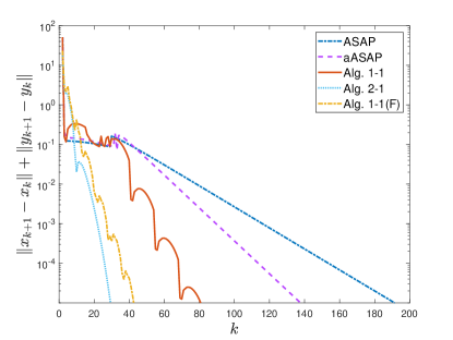
(a) Itakura-Saito distance

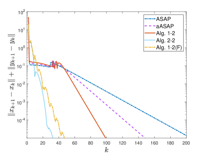
(b) squared Euclidean distance

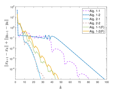
(c) Itakura-Saito and squared Euclidean distance

Figure 1: The value of $\|x_{k+1}-x_{k}\|+\|y_{k+1}-y_{k}\|$ versus the iteration numbers for different Bregman distance with different extrapolation parameter.

4.2 Sparse logistic regression

In this subsection, we apply our algorithms to solve the sparse logistic regression problem. It is an attractive extension to logistic regression as it can reduce overfitting and perform feature selection simultaneously. We consider the Capped-$l_{1}$ regularized logistic regression problem [37], defined as

$$\ \underset{x\in\mathbb{R}^{d}}{\min}\ \ \frac{1}{n}\sum_{i=1}^{n}\log(1+\exp(-b_{i}a_{i}^{T}x))+\lambda\sum_{j=1}^{d}\min(\left|x_{j}\right|,\theta),\ \ \theta>0,$$ (4.4)

where $x\in\mathbb{R}^{d}$, $a_{i}\in\mathbb{R}^{d}$, $b_{i}\in\left\{-1,1\right\},i=1,\dots,n.$

By the similar method as the former example, we transform (4.4) to

$$\ \underset{x,y\in\mathbb{R}^{d}}{\min} \frac{1}{n}\sum_{i=1}^{n}\log(1+\exp(-b_{i}a_{i}^{T}x))+\lambda\sum_{j=1}^{d}\min(\left|y_{j}\right|,\theta)$$ (4.5)

$$s.t.\ \ x=y,$$

which can be described as

$$\ \underset{x,y\in\mathbb{R}^{d}}{\min}\ \ \frac{1}{n}\sum_{i=1}^{n}\log(1+\exp(-b_{i}a_{i}^{T}x))+\lambda\sum_{j=1}^{d}\min(\left|y_{j}\right|,\theta)+\frac{\mu}{2}\left\|x-y\right\|^{2}.$$ (4.6)

Let

$$f(x)=\frac{1}{n}\sum_{i=1}^{n}\log(1+\exp(-b_{i}a_{i}^{T}x)),\ g(y)\equiv 0,$$ (4.7)

$$Q(x,y)=\lambda\sum_{j=1}^{d}\min(\left|y_{j}\right|,\theta)+\frac{\mu}{2}\left\|x-y\right\|^{2}.$$

It is easy to verify that all the functions satisfy the assumptions. However, when $n$ is large, $L_{\bigtriangledown f}$ is difficult to compute, we cannot determine the strong convexity modulus range of the Bregman function. So we need to use backtracking strategy to solve the problem. Let $\phi_{2}(y)=\frac{\eta}{2}\left\|y\right\|^{2}$, we can elaborate the $x$-subproblem and $y$-subproblem of our algorithms respectively as follows.

The $x$-subproblem in (4.6) corresponds to the following optimization problem

$$x_{k+1} \in\arg\min_{x\in\mathbb{R}^{d}}\left\{Q(x,\hat{y}_{k})+\left\langle\nabla f(\hat{x}_{k}),x\right\rangle+D_{\phi_{1}}(x,\hat{x}_{k})\right\}$$

$$=\arg\min_{x\in\mathbb{R}^{d}}\left\{\frac{\mu}{2}\left\|x-\hat{y}_{k}\right\|^{2}+\left\langle\nabla f(\hat{x}_{k}),x\right\rangle+D_{\phi_{1}}(x,\hat{x}_{k})\right\}.$$

The $y$-subproblem in (4.6) corresponds to

$$y_{k+1} \in\arg\min_{y\in\mathbb{R}^{d}}\left\{Q(x_{k+1},y)+\left\langle\nabla g(\hat{y}_{k}),y\right\rangle+D_{\phi_{2}}(y,\hat{y}_{k})\right\}$$

$$=\arg\min_{y\in\mathbb{R}^{d}}\left\{\frac{\mu}{2}\left\|x_{k+1}-y\right\|^{2}+\lambda\sum_{j=1}^{d}\min(\left|y_{j}\right|,\theta)+\frac{\eta}{2}\left\|y-\hat{y}_{k}\right\|^{2}\right\}$$

$$=\arg\min_{y\in\mathbb{R}^{d}}\left\{\lambda\sum_{j=1}^{d}\min(\left|y_{j}\right|,\theta)+\frac{\mu+\eta}{2}\left\|y-\frac{1}{\mu+\eta}(\eta\hat{y}_{k}+\mu x_{k+1})\right\|^{2}\right\}$$

$$=\arg\min_{y\in\mathbb{R}^{d}}\left\{\frac{\lambda}{\mu+\eta}\sum_{j=1}^{d}\min(\left|y_{j}\right|,\theta)+\frac{1}{2}\left\|y-\frac{1}{\mu+\eta}(\eta\hat{y}_{k}+\mu x_{k+1})\right\|^{2}\right\}.$$

For convenience, we set

$$\ h(t,y,u_{k})=\frac{\lambda}{t}\sum_{j=1}^{d}\min(\left|y_{j}\right|,\theta)+\frac{1}{2}\left\|y-u_{k}\right\|^{2},$$ (4.8)

where $t=\mu+\eta$, $u_{k}=\frac{1}{\mu+\eta}(\eta\hat{y}_{k}+\mu x_{k+1}).$ Then $h(t,y,u_{k})$ has a separable structure. It can be decomposed into $d$ one-dimensional subproblems. Let $\left(u_{k}\right)_{j}$ be the $j$-th component of $u_{k}$. Then each component of $y_{k+1}$ can be calculated from

$$\ \left(y_{k+1}\right)_{j}=\arg\min_{y_{j}\in\mathbb{R}}\left\{\frac{1}{2}\left(y_{j}-\left(u_{k}\right)_{j}\right)^{2}+\frac{\lambda}{t}\min(\left|y_{j}\right|,\theta)\right\},\ j=1,\dots,d,$$ (4.9)

where $\left(y_{k+1}\right)_{j}$ denotes the $j$-th component of $y_{k+1}$. Then (4.9) can be described as follows

$$\left\{\begin{array}[]{r@{\extracolsep{0.5ex}}r@{}r@{}r@{}r@{}r@{}r@{}}&\tilde{y}_{j}=\underset{y_{j}\in\mathbb{R}}{\arg\min}\ \frac{1}{2}\left(y_{j}-\left(u_{k}\right)_{j}\right)^{2}+\frac{\lambda}{t}\theta&\text{ if }\ \left|y_{j}\right|>\theta,\\ &\hat{y}_{j}=\underset{y_{j}\in\mathbb{R}}{\arg\min}\ \frac{1}{2}\left(y_{j}-\left(u_{k}\right)_{j}\right)^{2}+\frac{\lambda}{t}\left|y_{j}\right|&\text{ if }\ \left|y_{j}\right|<\theta.\end{array}\right.$$

Furthermore,

$$\left\{\begin{array}[]{r@{\extracolsep{0.5ex}}l@{}l@{}l@{}l@{}l@{}l@{}}&\tilde{y}_{j}&=&\text{sign}(\left(u_{k}\right)_{j})\max(\theta,|\left(u_{k}\right)_{j}|)&\text{ if }\ \left|y_{j}\right|>\theta,\\ &\hat{y}_{j}&=&\text{sign}(\left(u_{k}\right)_{j})\min(\theta,\max(0,|\left(u_{k}\right)_{j}|-\frac{\lambda}{t}))&\text{ if }\ \left|y_{j}\right|<\theta.\end{array}\right.$$

Set $h_{j}(t,y_{j},\left(u_{k}\right)_{j})=\frac{\lambda}{t}\min(\left|y_{j}\right|,\theta)+\frac{1}{2}\left\|y_{j}-\left(u_{k}\right)_{j}\right\|^{2}$. Then $\left(y_{k+1}\right)_{j}$ can be expressed by

$$\left(y_{k+1}\right)_{j}=\begin{cases}\tilde{y}_{j}&\text{ if }h_{j}(t,\tilde{y}_{j},\left(u_{k}\right)_{j})\leq h_{j}(t,\hat{y}_{j},\left(u_{k}\right)_{j}),\\ \hat{y}_{j}&\text{ otherwise.}\end{cases}$$

In the experiment, we take $n=500,d=200$ and the parameters of the problem are set as $\lambda=10^{-3},\theta=0.1\lambda$, which is the same as [38]. The backtracking parameters of the algorithm are set as $\rho=2,\delta=10^{-5}$. We selected the starting point for all algorithms randomly and use

$$E_{k}=\|x_{k+1}-x_{k}\|+\|y_{k+1}-y_{k}\|<10^{-5}$$

as the stopping criteria. In the numerical results, “Iter.” denotes the number of iterations. “Time” denotes the CPU time. “Extrapolation” records the number of taking extrapolation step.

In order to show the effectiveness of the proposed algorithms, we compare our algorithms with ASAP [17] and aASAP [7]. The extrapolation parameter of aASAP is $\alpha_{k}=0.3$. In Algorithm 1, we set $\alpha_{k}=0.3,\beta_{k}=0.2$. And we also take extrapolation parameter dynamically updating with $\alpha_{k}=\beta_{k}=\frac{k-1}{k+2}$. For Algorithm 2, we set $\alpha_{0}=0.3,\beta_{0}=0.2$ as the initial extrapolation parameter and $t=1.5,\beta_{\max}=0.499$. We also use “Alg. 1-i” and “Alg. 2-i” to denote Algorithm 1 and Algorithm 2 with $\phi_{1}(x)=\varphi_{i}(x)(1\leq i\leq 2)$, respectively, where extrapolation parameter $\alpha_{k}=0.3,\beta_{k}=0.2$. We use “Alg. 1-i(F)” and “Alg. 2-i(F)” to denote Algorithm 1 and Algorithm 2 with $\phi_{1}(x)=\varphi_{i}(x)(1\leq i\leq 2)$, respectively, where extrapolation parameter $\alpha_{k}=\beta_{k}=\frac{k-1}{k+2}$.

Figure 2 shows the performance of different algorithms. We also list the iteration number, the CPU time, and the extrapolation number on the test set of each algorithm in Table 2. Figure 2 (a) and (b) reports the result of different extrapolation parameter, respectively. It shows that Algorithm 2 with adaptive extrapolation parameters performs the best among all algorithms. Figure 2 (c) reports the result of different Bregman distance. It shows that the Itakura-Saito distance have computational advantage than the squared Euclidean distance.

We also use BB rule improves the computational efficiency of each algorithm. The symbol in Table 3 and Figure 3 “$\sim$BB” means that the algorithm adopts the BB rule with lower bound of $t_{\min}=1.3$ in backtracking process. It shows that using BB rule to initialize the stepsize can improve the efficiency of all algorithms.

Table 2: Numerical results of different Bregman distance with different extrapolation parameter

Itakura-Saito distance					squared Euclidean distance
Algorithm	Iter.	Time(s)	Extrapolation		Algorithm	Iter.	Time(s)	Extrapolation
ASAP	39	9.3456	38		ASAP	71	18.3569	70
aASAP	35	8.3227	34		aASAP	56	14.0903	55
Alg. 1-1	29	6.9867	21		Alg. 1-2	43	11.0023	39
Alg. 2-1	15	3.4024	7		Alg. 2-2	23	6.1576	16
Alg. 1-1(F)	19	5.5435	8		Alg. 1-2(F)	33	7.9012	20

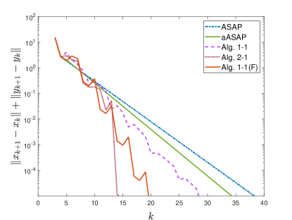
(a) Itakura-Saito distance

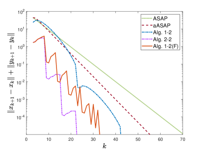
(b) squared Euclidean distance

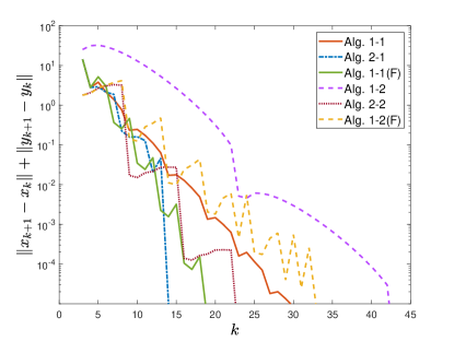
(c) Itakura-Saito and squared Euclidean distance

Figure 2: The value of $\|x_{k+1}-x_{k}\|+\|y_{k+1}-y_{k}\|$ versus the iteration numbers for Algorithm 1 with different extrapolation parameter.

Table 3: Numerical results of different Bregman distance with different extrapolation parameter

Itakura-Saito distance					squared Euclidean distance
Algorithm	Iter.	Time(s)	Extra.		Algorithm	Iter.	Time(s)	Extra.
ASAP$\sim$BB	15	4.3476	14		ASAP$\sim$BB	25	6.4702	24
aASAP$\sim$BB	14	4.0324	13		aASAP$\sim$BB	21	6.0604	20
Alg. 1-1$\sim$BB	13	3.9198	7		Alg. 1-2$\sim$BB	19	5.3523	10
Alg. 2-1$\sim$BB	9	2.9745	5		Alg. 2-2$\sim$BB	15	4.1270	8
Alg. 1-1(F)$\sim$BB	11	3.5435	6		Alg. 1-2(F)$\sim$BB	17	4.9352	9

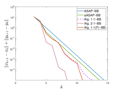
(a) Itakura-Saito distance

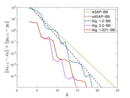
(b) squared Euclidean distance

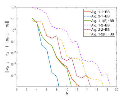
(c) Itakura-Saito and squared Euclidean distance

Figure 3: The value of $\|x_{k+1}-x_{k}\|+\|y_{k+1}-y_{k}\|$ versus the iteration numbers for Algorithm 1 with different extrapolation parameter.

5 Conclusion

In this paper, we introduce a two-step inertial Bregman alternating structure-adapted proximal gradient descent algorithm for solve nonconvex and nonsmooth nonseparable optimization problem. Under some assumptions, we proved that our algorithm is a descent method in sense of objective function values, and every cluster point is a critical point of the objective function. The convergence of proposed algorithms are proved if the objective function satisfies the Kurdyka–Łojasiewicz property. Furthermore, if the desingularizing function has the special form, we also established the linear and sub-linear convergence rates of the function value sequence generated by the algorithm. In addition, we also proposed a backtracking strategy with BB method to make our algorithms more flexible when the Lipschitz constant is unknown or difficult to compute. In numerical experiments, we apply different Bregman distance to solve nonconvex quadratic programming and sparse logistic regression problem. Numerical results are reported to show the effectiveness of the proposed algorithm.

References

- [1] Nikolova M., Ng M.K., Zhang S.Q., Ching W.K., Efficient reconstruction of piecewise constant images using nonsmooth nonconvex minimization, SIAM J. Imaging Sci., 2008, 1(1), 2-25.
- [2] Gu S.H., Zhang L., Zuo W.M., Feng X.C., Weighted nuclear norm minimization with application to image denoising, In: Proceedings of the IEEE Conference on Computer Vision and Pattern Recognition (CVPR), 2014, 2862-2869.
- [3] Bian W., Chen X.J., Linearly constrained non-Lipschitz optimization for image restoration, SIAM J. Imaging Sci., 2015, 8(4), 2294-2322.
- [4] Paatero, P., Tapper, U., Positive matrix factorization: a nonnegative factor model with optimal utilization of error estimates of data values, Environmetrics 5, 1994, 111-126.
- [5] Lee, D.D., Seung, H.S., Learning the parts of objects by nonnegative matrix factorization, Nature 401, 1999, 788-791.
- [6] Bot R.I., Csetnek E.R., Vuong P.T., The forward-backward-forward method from continuous and discrete perspective for pseudo-monotone variational inequalities in hilbert spaces, Eur. J. Oper. Res., 2020, 49-60.
- [7] Xu L.L., Xin Y., Vuong P.T., Some accelerated alternating proximal gradient algorithms for a class of nonconvex nonsmooth problems, J. Glob. Optim., 2022, https://doi.org/10.1007/s10898-022-01214-3.
- [8] Attouch H., Bolte J., Svaiter B.F., Convergence of descent methods for semi-algebraic and tame problems: proximal algorithms, forward-backward splitting, and regularized Guass-Seidel methods, Math. Program., 2013, 137, 91-129.
- [9] Donoho D.L., Compressed sensing, IEEE Trans. Inform. Theory, 2006, 4, 1289-1306.
- [10] Bertsekas D.P., Nonlinear programming, J. Oper. Res. Soc., 1977, 48, 334-334.
- [11] Beck A., Tetruashvili L., On the convergence of block coordinate descent type methods, SIAM J. Optim., 2013, 23, 2037-2060.
- [12] Auslender A., Asymptotic properties of the Fenchel dual functional and applications to decomposition problems, J. Optim. Theory Appl., 1992, 73(3), 427-449.
- [13] Attouch H., Bolte J., Redont P., Soubeyran A., Proximal alternating minimization and projection methods for nonconvex problems: an approach based on the Kurdyka–Łojasiewicz inequality, Math. Oper. Res., 2010, 35, 438-457.
- [14] Attouch, H., Redont, P., Soubeyran, A., A new class of alternating proximal minimization algorithms with costs-to-move, SIAM J. Optim. 2007, 18, 1061-1081.
- [15] Xu, Y., Yin, W., A block coordinate descent method for regularized multiconvex optimization with applications to nonnegative tensor factorization and completion, SIAM J. Imaging Sci, 2013, 6, 1758-1789.
- [16] Bolte J., Sabach S., Teboulle M., Proximal alternating linearized minimization for nonconvex and nonsmooth problems, Math. Program., 2014, 146, 459-494.
- [17] Nikolova M., Tan P., Alternating structure-adapted proximal gradient descent for nonconvex block-regularised problems, SIAM J. Optim., 2019, 29(3), 2053-2078.
- [18] Ochs P., Chen Y., Brox T., and Pock T., iPiano: Inertial proximal algorithm for nonconvex optimization, SIAM J. Imaging Sci., 2014, 7(2), 1388-1419.
- [19] Boţ R.I., Csetnek E.R., An inertial Tseng’s type proximal algorithm for nonsmooth and nonconvex optimization problems, J. Optim. Theory Appl., 2016, 171(2), 600-616.
- [20] Polyak B.T., Some methods of speeding up the convergence of iteration methods, USSR Comput. Math. Math. Phys., 1964, 4, 1-17.
- [21] Alvarez, F., Attouch, H., An inertial proximal method for maximal monotone operators via discretization of a nonlinear oscillator with damping. Set-Valued Anal. 2001, 9(1), 3-11.
- [22] Pock T., Sabach S., Inertial proximal alternating linearized minimization (iPALM) for nonconvex and nonsmooth problems, SIAM J. Imaging Sci., 2017, 9, 1756-1787.
- [23] Gao X., Cai X.J., Han D.R., A Gauss-Seidel type inertial proximal alternating linearized minimization for a class of nonconvex optimization problems, J. Glob. Optim., 2020, 76, 863-887.
- [24] Zhao J., Dong Q.L., Michael Th.R., Wang F.H., Two-step inertial Bregman alternating minimization algorithm for nonconvex and nonsmooth problems, J. Glob. Optim., 2022, 84, 941-966.
- [25] Chao M.T., Nong F.F., Zhao M.Y., An inertial alternating minimization with Bregman distance for a class of nonconvex and nonsmooth problems, J. Appl. Math. Comput., 2023, 69, 1559-1581.
- [26] Mordukhovich B., Variational Analysis and Generalized Differentiation, I: Basic Theory. Grundlehren der Mathematischen Wissenschaften, Vol. 330. Springer-Verlag, Berlin, 2006.
- [27] Rockafellar R.T., Wets R., Variational analysis, Grundlehren der Mathematischen Wissenschaften, Vol. 317. Springer, Berlin, 1998.
- [28] Rockafellar, R.T., Wets, J.B.: Variational Analysis. Springer, New York, 1998.
- [29] Bertsekas D.P., Tsitsiklis J.N., Parallel and Distributed Computation: Numerical Methods, Prentice hall, Englewood Cliffs, NJ, 1989.
- [30] Wang F., Cao W., Xu Z., Convergence of multi-block Bregman ADMM for nonconvex composite problems, Sci. China Inf. Sci., 2018, 61, 122101.
- [31] Li, H., Lin, Z., Accelerated proximal gradient methods for nonconvex programming, In: Advances in Neural Information Processing Systems, pp,2015, 379-387.
- [32] Li, Q., Zhou, Y., Liang, Y., Varshney, P.K., Convergence analysis of proximal gradient with momentum for nonconvex optimization. In: Proceedings of the 34th International Conference on Machine Learning, 2017,2111-2119.
- [33] Barzilai, J., Borwein, J.M., Two-point step size gradient methods, IMA J. Numer. Anal. 1998, 8, 141-148.
- [34] Attouch, H., Bolte, J.: On the convergence of the proximal algorithm for nonsmooth functions involving analytic features. Math. Program. Ser. B, 2009, 116, 5-16.
- [35] Li, H., Lin, Z.: Accelerated proximal gradient methods for nonconvex programming. In: Advances in Neural Information Processing Systems, pp., 2015, 379-387.
- [36] Li, Q., Zhou, Y., Liang, Y., Varshney, P.K., Convergence analysis of proximal gradient with momentum for nonconvex optimization. In: Proceedings of the 34th International Conference on Machine Learning, 2017, 2111-2119.
- [37] Zhang, T., Analysis of multi-stage convex relaxation for sparse regularization, J. Mach. Learn. Res. 2010, 11, 1081-1107.
- [38] Gong, P., Zhang, C., Lu, Z., Huang, J., Ye, J., A general iterative shrinkage and thresholding algorithm for nonconvex regularized optimization problems. In: International Conference on Leadership and Management, 2013, 37-45.