Exploring Quantum Synchronization with a Composite Two-Qubit Oscillator

Abstract

Synchronization has recently been explored deep in the quantum regime with elementary few-level quantum oscillators such as qudits and weakly pumped quantum Van der Pol oscillators. To engineer more complex quantum synchronizing systems, it is practically relevant to study composite oscillators built up from basic quantum units that are commonly available and offer high controllability. Here, we consider a minimal model for a composite oscillator consisting of two interacting qubits coupled to separate baths, for which we also propose and analyze an implementation on a circuit quantum electrodynamics platform. We adopt a ‘microscopic’ and ‘macroscopic’ viewpoint and study the response of the constituent qubits and of the composite oscillator when one of the qubits is weakly driven. We find that the phase-locking of the individual qubits to the external drive is strongly modified by interference effects arising from their mutual interaction. In particular, we discover a phase-locking blockade phenomenon at particular coupling strengths. Furthermore, we find that interactions between the qubits can strongly enhance or suppress the extent of synchronization of the composite oscillator to the external drive. Our work demonstrates the potential for assembling complex quantum synchronizing systems from basic building units, which is of pragmatic importance for advancing the field of quantum synchronization.

I Introduction

Synchronization is at the heart of a variety of phenomena in nature and finds important practical applications, e.g. in the working of pacemakers and lasers [1]. At its core, synchronization is the tendency of a self-powered, or self-sustained oscillator (SSO) to lock to an external phase reference. Quantum synchronization explores how the synchronizing tendency of SSOs is affected by the strong quantum mechanical effects that arise when they are scaled down in size and energy [2, 3, 4, 5, 6, 7, 8, 9, 10, 11, 12, 13, 14, 15, 16, 17, 18, 19, 20].

A quantum SSO can be realized as the low occupation limit of a classical SSO or as a finite-dimensional system where only a few states are available even in principle. An example for the former is a weakly pumped Van der Pol oscillator, such that its mean occupation number is of order unity [2, 3, 4, 5]. On the other hand, a qudit with gain and damping serves as a realization of a finite dimensional quantum SSO [6, 7, 8, 9].

An important problem in quantum synchronization research is to understand the response of elementary quantum SSOs to external driving or when two (or more) such SSOs are coupled. Similar to classical systems, quantum SSOs exhibit a characteristic Arnold Tongue like behaviour [7], where the extent of synchronization increases with drive strength and decreases as the drive frequency is detuned from the natural frequency of the oscillator. However, quantum SSOs also display quantum features such as entanglement [4, 6], and quantum interference effects that lead to synchronization blockade [10, 11, 12]. Crucially, the presence of quantum effects depends on the details of the gain and damping mechanisms that power the SSO, making their interplay an important ingredient in the study of quantum synchronization. Furthermore, quantum synchronization has recently gained experimental relevance with the demonstration of synchronization in a vapor of Rb atoms [13], in nuclear spin systems [14], as well as by a digital simulation on a quantum computer [15].

In order to further explore quantum effects and potential applications of quantum synchronization, we require the ability to realize a wider variety of quantum SSOs whose properties can be externally tuned. As a result, it is practically relevant to consider quantum SSOs composed of building blocks that are commonly available in current experimental platforms and also offer a high degree of controllability. As we demonstrate, such a ‘bottom-up’ approach provides an avenue to assemble quantum synchronizing systems with desired features by tuning the properties of the constituent building blocks.

In this paper, we introduce a minimal model of a composite quantum SSO made from two interacting qubits. The qubits are each coupled to separate thermal baths that provide local gain and damping to power the SSO. Crucially, we allow for baths with positive (damping dominated) and negative (gain dominated) temperatures. By varying the local gain and damping rates, and the qubit-qubit coupling strength, the properties of the composite oscillator such as its intrinsic steady state and relaxation timescales can be tuned. We emphasize that, in contrast to previous studies of few-level quantum systems [6], here we do not focus on the mutual synchronization of two quantum units when they are perturbatively coupled. Instead, we consider strong coupling between the two qubits and consider the two-qubit system as a single composite oscillator that is in turn perturbatively driven by an external drive.

The exploration of such a composite system involves understanding the ‘microscopic’ behavior at the level of individual constituents as well as the ‘macroscopic’ behavior of the system as a whole. Accordingly, we study the response of this system when one of the qubits is weakly driven from two viewpoints. First, we study how the tendency of the individual qubits to phase lock to the external drive is modified by virtue of their mutual interaction. In particular, we find that, as the coupling strength increases, the qubits undergo an abrupt $\pi$ phase shift in the phase they develop relative to the drive, with signatures of phase-locking completely vanishing at a particular coupling strength. Next, we explore the tendency of the composite oscillator, as a whole, to synchronize to the drive, using a recently introduced generalized measure of quantum synchronization [16]. Interestingly, we uncover parameter regimes where the qubit-qubit interaction can lead to strong enhancement as well as suppression of quantum synchronization.

In line with our motivation to study experimentally feasible systems, we propose a realization of our model on a circuit quantum electrodynamics (QED) platform. The qubits are encoded in two transmons that are coupled to each other via a tunable coupling element. While damping channels are intrinsic to the transmons, we propose to engineer gain channels by using appropriate drives and auxiliary resonators. We also perform master equation simulations of this proposed implementation to demonstrate its feasibility.

This paper is organized as follows. In Section II, we introduce our two-qubit oscillator model and discuss the metrics we use to quantify the phase locking of individual qubits and the synchronization of the composite system. We use these metrics to study the two-qubit oscillator as the system parameters are varied in Section III. In Section IV, we propose and simulate a circuit QED realization of the two-qubit oscillator. We conclude with a summary and outlook in Section V. Relevant additional details and extensions are provided in the form of Appendices. In particular, our model can be generalized to higher dimensional spins, which we illustrate with the example of a two-qutrit oscillator in Appendix D.

II Model and Methods

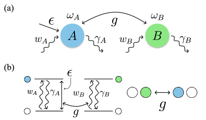
Figure 1: The composite two-qubit oscillator. (a) Schematic showing two interacting qubits, with each qubit coupled to a thermal bath. Additionally, qubit $A$ is weakly and coherently driven with strength $\epsilon$. (b) Energy level diagram showing the gain and damping channels, and the exchange interaction of the qubits. The right panel illustrates the flip-flop of excitations under the exchange interaction. The white (colored) circles represent the ground (excited) states of the two qubits.

In this section, we first describe the system under study. Subsequently, we introduce the metrics we use to quantify the phase locking of individual qubits and the synchronization of the composite oscillator.

II.1 Model

The model we consider is shown in Fig. 1(a) and is broadly applicable to a two-qudit oscillator. We consider two spin-$S$ systems (qudits) $A$ and $B$ with natural frequencies $\omega_{A}$ and $\omega_{B}$, interacting via an exchange interaction with strength $g$. Additionally, qudit $A$ is weakly and coherently driven by an external drive with frequency $\omega_{d}$ and strength $\epsilon$. In the frame rotating with frequency $\omega_{d}$, the Hamiltonian for the system is given by ($\hbar=1$)

$$\hat{H}_{\mathrm{tot}} = \Delta_{d}\hat{S}_{A}^{z}+\left(\Delta_{d}+\Delta_{q}\right)\hat{S}_{B}^{z}$$ (1)

$$+\frac{\epsilon}{2}\left(\hat{S}^{+}_{A}+\hat{S}^{-}_{A}\right)+\frac{g}{2}\left(\hat{S}^{+}_{A}\hat{S}^{-}_{B}+\hat{S}^{-}_{A}\hat{S}^{+}_{B}\right),$$

where $\Delta_{d}=\omega_{A}-\omega_{d}$ and $\Delta_{q}=\omega_{B}-\omega_{A}$ are respectively the drive and relative qudit detunings. For each qudit, the operator $\hat{S}^{z}$ corresponds to the $z$ component of the spin and has eigenvectors $\ket{S,m}$ that satisfy $\hat{S}^{z}\ket{S,m}=m\ket{S,m}$. The operators $\hat{S}^{+},\hat{S}^{-}$ are raising and lowering operators that transform the states according to $\hat{S}^{\pm}\ket{S,m}=\sqrt{(S\mp m)(S\pm m+1)}\ket{S,m\pm 1}$.

Furthermore, each qudit is coupled to a thermal bath which leads to loss (gain) of qudit excitations at rates $\gamma_{j}$ ($w_{j}$) with $j=A,B$. In particular, $\gamma_{j}>w_{j}$ ($\gamma_{j}<w_{j}$) corresponds to a positive (negative) temperature bath dominated by loss (gain). These two regimes occur on either side of an infinite temperature bath corresponding to $w_{j}=\gamma_{j}$. The dynamics of the composite system can then be described by the master equation

$$\frac{d\hat{\rho}}{dt} = -i\left[\hat{H}_{\mathrm{tot}},\hat{\rho}\right]$$ (2)

$$+\sum_{j={A,B}}\mathfrak{D}[\sqrt{w_{j}}\hat{S}_{j}^{+}]\hat{\rho}+\sum_{j={A,B}}\mathfrak{D}[\sqrt{\gamma_{j}}\hat{S}_{j}^{-}]\hat{\rho},$$

where $\mathfrak{D}[\hat{O}]\hat{\rho}=\hat{O}\hat{\rho}\hat{O}^{\dagger}-\frac{1}{2}\hat{O}^{\dagger}\hat{O}\hat{\rho}-\frac{1}{2}\hat{\rho}\hat{O}^{\dagger}\hat{O}$ is the Lindblad dissipator.

In Fig. 1(b), we illustrate the particular instance of this model when $A$ and $B$ are qubits, which will be the primary focus of this work. For discussing the results in Sec. III, we use as a characteristic frequency the total relaxation rate $\Gamma_{j}$ of a single qubit, defined as

$$\Gamma_{j}=\gamma_{j}+w_{j},\;j=A,B.$$ (3)

II.2 Phase locking metric for individual qubits

In Sec. III.1, we study the phase locking of the individual qubits to a weak external drive applied on one of them. The metric we use to quantify phase locking is the off-diagonal element, or coherence, of the steady-state reduced density matrix of each qubit. The choice of this metric is based on the phase space representation of the individual qubits using the Husimi $Q$ function, which we define here with respect to the $SO(3)$ coherent states . For a general spin-$S$ system, the $Q$ function is defined as the overlap

$$Q_{S,\hat{\rho}}(\theta,\varphi)=\bra{\theta,\varphi}\hat{\rho}\ket{\theta,\varphi}.$$ (4)

Here, $\ket{\theta,\varphi}$ are the $SO(3)$ coherent states for a spin-$S$ system, which are defined via rotations of the state $\ket{S,m=S}$ as $\ket{\theta,\varphi}=e^{i\varphi\hat{S}^{z}}e^{i\theta\hat{S}^{y}}\ket{S,m=S}$ [22]. The angles $\theta,\varphi$ respectively correspond to the polar and azimuthal angles on a generalized Bloch sphere. The $Q$ function therefore serves as a tool to visualize the state of the system on the surface of this sphere.

For qubits, the $Q$ function can be expressed as

$$Q_{\frac{1}{2},\hat{\rho}}(\theta,\varphi) = \frac{1}{2}+\langle\hat{S}^{z}\rangle\cos\theta+\mathrm{Re}[\langle\hat{S}^{+}\rangle e^{-i\varphi}]\sin\theta.$$

The external drive introduces a nontrivial azimuthal phase distribution by establishing coherences in the system such that $\langle\hat{S}^{+}\rangle\neq 0$. This leads to a marginal distribution $P(\varphi)=(1/2\pi)\int_{0}^{\pi}d\theta\sin\theta\;Q_{\frac{1}{2},\hat{\rho}}(\theta,\varphi)$ for $\varphi$ that deviates from a uniform distribution. In Sec. III.1, we visualize this deviation by plotting the quantity $\delta P(\varphi)$ defined as

$$\delta P(\varphi)=P(\varphi)-\frac{1}{2\pi}=\frac{1}{4}\mathrm{Re}[\langle\hat{S}^{+}\rangle e^{-i\varphi}].$$ (6)

Therefore, the phase-locking of individual qubits can be studied by probing the magnitude of the off-diagonal element of their reduced density matrices.

For a general spin-$S$ system, the $Q$ function can be decomposed into a sum of expectation values of spherical tensors, which is useful in the study of phase locking in higher dimensional spin systems. We discuss this in more detail in Appendix A.

II.3 Synchronization measure for composite oscillator

In Sec. III.2, we study the synchronization of the composite two-qubit oscillator, as a whole, when one of the qubits is weakly driven. For this study, we use an information theoretic measure of synchronization proposed in Ref. [16]. This metric is system agnostic, which makes it an attractive choice to study synchronisation of composite systems, where quasiprobability distributions may be inconvenient to compute as well as interpret.

The central idea underlying this metric is to quantify synchronization as the deviation of the steady state $\hat{\rho}$ in the presence of the external drive from an appropriate limit cycle state $\hat{\rho}_{\mathrm{lim}}$ (described below), measured using a suitable measure of distance $\mathcal{D}$. In particular, when $\hat{\rho}_{\mathrm{lim}}$ is full rank, the distance $\mathcal{D}$ is taken as the relative entropy

$$\mathcal{D}\equiv S(\hat{\rho}||\hat{\rho}_{\mathrm{lim}})=\mathrm{Tr}\left[\hat{\rho}\log(\hat{\rho})-\hat{\rho}\log(\hat{\rho}_{\mathrm{lim}})\right].$$ (7)

The limit cycle state $\hat{\rho}_{\mathrm{lim}}$ is the closest state to $\hat{\rho}$ which does not have the coherences induced by the drive. In general, the limit cycle state $\hat{\rho}_{\mathrm{lim}}$ is not just the steady state of the system when the drive is turned off. The reason is that, while the drive generally induces changes in populations as well as coherences, a synchronization metric must be sensitive only to the buildup of coherences. This subtlety is accounted for by minimizing $\mathcal{D}$ over an appropriate set, $\Sigma$, of ‘candidate’ limit cycle states to obtain the synchronization measure, i.e.

$$\Omega(\hat{\rho})=\min_{\hat{\rho}_{\mathrm{lim}}\in\Sigma}\mathcal{D}(\hat{\rho},\hat{\rho}_{\mathrm{lim}}),$$ (8)

where the measure $\Omega(\hat{\rho})$ is called the relative entropy of synchronization.

The set $\Sigma$ of candidate limit cycle states is chosen according to the system being studied. For our system, a natural choice of $\Sigma$ is the set of states that are diagonal in the eigenbasis $\{\ket{\lambda_{j}}\}$ of the steady state $\hat{\rho}_{u}$ of the undriven oscillator, since synchronization to the external drive occurs via the buildup of coherences between the different bases $\{\ket{\lambda_{j}}\}$. For the particular case of such diagonal limit cycle states, the minimization in Eq. (8) can be performed analytically and $\Omega(\hat{\rho})$ reduces to [16]

$$\Omega(\hat{\rho})=S(\hat{\rho}_{\mathrm{diag}})-S(\hat{\rho}).$$ (9)

Here, $S(\hat{\rho})=\mathrm{Tr}\left[-\hat{\rho}\log(\hat{\rho})\right]$ is the von Neumann entropy and $\hat{\rho}_{\mathrm{diag}}$ is a state diagonal in $\{\ket{\lambda_{j}}\}$, obtained by simply deleting all the off-diagonal elements of $\hat{\rho}$ expressed in this basis.

We note that, for a system of the kind considered here, Ref. [16] prescribes to choose $\Sigma$ as a set of so-called ‘partially-coherent’ candidate limit cycle states. In Appendix B, we show that such a choice leads to identical results as the ones we have obtained using diagonal limit cycle states, and provide an intuitive explanation for why this is the case.

II.4 Qualitative expectations from the collective spin picture

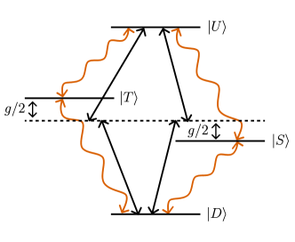
Figure 2: Collective spin representation of the two-qubit oscillator using the singlet and triplet basis states.

Before turning to the results, we provide some intuition for the behavior of the metrics introduced in the previous two subsections. Both the metrics are sensitive to the coherences established in the two-qubit system as a result of the weak external drive, but in different ways. To discuss them in a common framework, we consider the two-qubit oscillator in the basis formed by the eigenstates of the undriven system Hamiltonian, i.e. Eq. (1) with $\epsilon=0$ (see Fig. 2). In addition, we also assume $\Delta_{d}\approx\Delta_{q}\approx 0$ for the following discussion. Then, the eigenstates are the usual singlet and triplet basis states corresponding to the collective spin of the two qubits, which we denote using the $m_{A},m_{B}$ quantum numbers of the two qubits as $\ket{D}=\ket{-1/2,-1/2},\ket{U}=\ket{1/2,1/2},\ket{T}=(\ket{1/2,-1/2}+\ket{-1/2,1/2})/\sqrt{2}$ and $\ket{S}=(\ket{1/2,-1/2}-\ket{-1/2,1/2})/\sqrt{2}$.

The external drive is weak and, for $\Delta_{d}\approx 0$, it is near resonance with the bare transition frequency of qubit $A$. In the collective spin picture, this drive translates to simultaneously driving four transitions as depicted by the black arrows in Fig. 2. This can be seen by expressing the drive term in Eq. (1) in the collective spin basis, using the relation

$$\hat{S}_{A}^{+}=\frac{1}{\sqrt{2}}\left(\ket{U}\bra{T}-\ket{U}\bra{S}+\ket{T}\bra{D}+\ket{S}\bra{D}\right).$$ (10)

For strong qubit-qubit interaction, i.e. $g/\Gamma\gg 1$ ($\Gamma_{A}\sim\Gamma_{B}\sim\Gamma$), the states $\ket{T},\ket{S}$ are shifted from the bare resonance by $\pm g/2$ and hence all four transitions are driven off-resonantly. Hence, the coherence established in the system decreases and consequently the phase locking and synchronization metrics asymptotically decay to zero as $g\rightarrow\infty$.

In the intermediate regime where $g/\Gamma\sim 1$, one can expect a complex interplay of qubit-qubit interactions, and the gain and loss channels, that leads to non-trivial effects on the metrics. In the collective spin picture, the effect of the local thermal baths is to induce correlated decay between the various states, depicted by the orange arrows in Fig. 2. This can be seen by expressing the $\hat{S}_{A}^{\pm},\hat{S}_{B}^{\pm}$ operators analogous to Eq. (10). The simultaneous driving of four transitions and the correlated decay among the collective spin states leads to mixing of the coherences between the various pairs of states connected by the drive, leading to strong interference effects.

As illustrated by Eq. (10), the phase locking metrics, given by $\lvert\langle\hat{S}_{j}^{+}\rangle\rvert,j=A,B$, are obtained by a phase-sensitive addition of the coherences between the collective spin states. The resulting value thus depends on the relative phase of the coherences and their magnitudes, and for instance, can vanish under certain conditions. We will demonstrate and investigate such ‘zero-crossings’ in Sec. III.1. On the other hand, the synchronization metric captures the overall build-up of coherences in the system and, qualitatively speaking, is sensitive to the magnitude of the individual coherences between the different pairs of states. However, as mentioned before, interference effects strongly modify even the magnitudes of the individual coherences, which can lead to an enhancement or suppression of the synchronization metric in the composite system compared to the non-interacting case ($g=0$). This will be explored in Sec. III.2.

III Results

In Sec. III.1, we study the response of the individual qubits to the external drive and explore the role of the system parameters on their tendency to phase lock to this drive. Subsequently, in Sec. III.2, we consider the two-qubit oscillator as a composite oscillator and study its collective response to the drive. An extension of this study to a two-qutrit oscillator is discussed in Appendix D. In the following, we take the total relaxation rate [see Eq. (3)] of each qubit to be the same, i.e. $\Gamma_{A}=\Gamma_{B}=\Gamma$, and report frequency values ($w_{j},\gamma_{j},g,\Delta_{d},\Delta_{q},\epsilon,j=A,B$) in units of $\Gamma$, so that $\gamma_{j}=1-w_{j}$ when expressed in these units.

III.1 Phase locking of individual qubits

As described in Sec. II.2, the phase locking of a qubit is quantified by the magnitude of $\langle\hat{S}^{+}\rangle$, which is just the off-diagonal element, or coherence, of the reduced density matrix of the qubit. In Fig. 3(a), we plot $\lvert\langle\hat{S}^{+}\rangle\rvert$ normalized to the drive strength $\epsilon$ for both qubits as the qubit-qubit coupling strength $g$ is varied. Here, we have set $\Delta_{d}=\Delta_{q}=0$, i.e. the frequencies of the drive and the two qubits are taken to be equal. As $g$ increases, the extent of phase-locking of qubit $A$ decreases and eventually vanishes completely at a particular strength $g_{0,A}$ indicated by the purple star. In the case of qubit $B$, we observe that it develops a non-zero measure of phase-locking, even though it is not directly driven, by virtue of its coupling with qubit $A$. Interestingly, the coherence of qubit $B$ also vanishes completely at a specific coupling strength $g_{0,B}$ (orange star). Finally, at large values of $g$, the coherence of either qubit approaches zero asymptotically, which can be understood as the result of off-resonant driving in the collective spin picture (Sec. II.4).

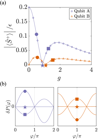
Figure 3: Phase locking of the individual qubits. (a) $\lvert\langle\hat{S}^{+}\rangle\rvert/\epsilon$ for qubits A and B versus the coupling strength $g$ between the two qubits. Here, we choose $w_{A}=0.4,\gamma_{A}=0.6$ and $w_{B}=0.75,\gamma_{B}=0.25$. Markers (lines) are numerical (analytical) results. (b) The variation in the azimuthal phase distribution $\delta P(\varphi)$ [see Eq. (6)] for qubit $A$ (left) and qubit $B$ (right) at the coupling strengths indicated in panel (a).

The complete vanishing of $\lvert\langle\hat{S}_{j}^{+}\rangle\rvert,j=A,B$ at $g_{0,j}$ corresponds to a zero crossing of the quantity $\langle\hat{S}_{j}^{+}\rangle$, which in turn marks a $\pi$ phase shift in the locking of the corresponding qubit to the drive. We demonstrate this in Fig. 3(b), where we plot the variation in the azimuthal phase distribution $\delta P(\varphi)$ [see Eq. (6)] for the two qubits at coupling strengths before, at, and after the zero-crossing point. The distribution for either qubit is flat right at the zero crossing point while a $\pi$ phase shift is evident in the distributions before and after this point.

The zero-crossing phenomenon occurs as a result of destructive interference from multiple drive pathways. For instance, in the case of qubit $A$, multiple pathways arise from the direct external driving and the feedback from qubit $B$ as a result of the coupling. Alternatively, one can also interpret this phenomenon as a destructive addition of coherences in the collective spin picture, as discussed in Sec. II.4. This phenomenon is intriguing because, for either qubit, the reduced density matrix at its respective zero-crossing point has an azimuthal phase symmetry as seen by the flat profile of $\delta P(\varphi)$, a remarkable feature given that the external drive explicitly breaks this symmetry in the system Hamiltonian (1). Hence, in the following we will explore the parameter regimes where such a zero crossing can be observed.

III.1.1 Zero crossing: Interplay of gain and loss rates

The existence of a zero-crossing point is dependent on the temperatures of the local thermal baths coupled to each qubit. In order to rigorously determine the parameter regime where a zero-crossing can be observed, we first obtain an analytic expression for $\lvert\langle\hat{S}_{j}^{+}\rangle\rvert,j=A,B$ as a function of the coupling strength $g$, treating the drive strength $\epsilon$ as a perturbation. The details of this approach are presented in Appendix C. As shown in Fig. 3(a), the analytical expression (solid lines) is in excellent agreement with numerical results (markers). Next, we determine the existence of a zero-crossing point by solving for the coupling strength $g_{0,j}$ where this expression vanishes.

In Fig. 4, we explore the existence of a zero-crossing point for each qubit as their gain rates (and consequently their bath temperatures) are varied. The color indicates the value of $g_{0}$, while the regions in white correspond to bath parameters where a zero-crossing point does not exist. We observe that, for both qubits, a zero-crossing point only exists when the baths are inverted with respect to each other, i.e. when $w_{A}>\gamma_{A}$ and $w_{B}<\gamma_{B}$ or vice-versa. In other words, qubit $A$ (qubit $B$) must be coupled to a negative (positive) temperature bath or vice-versa. While this is a necessary condition to observe a zero crossing in qubit $A$, it is both necessary and sufficient in the case of qubit $B$. Furthermore, except in a narrow band (highlighted in red) for qubit $A$ where $g_{0,A}$ rapidly increases, the zero crossing typically occurs for values of $g_{0,j}\sim\mathcal{O}(1),j=A,B$, corresponding to the regime where qubit-qubit coupling strengths are comparable to the gain and loss rates of the qubits.

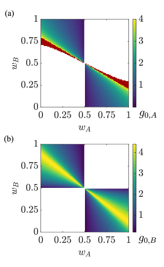
Figure 4: Bath parameters over which a zero crossing can be observed. The panels show the coupling strength at which the zero crossing occurs for (a) qubit $A$, and (b) qubit $B$, as $w_{A},w_{B}$ are scanned while fixing $\gamma_{A}+w_{A}=\gamma_{B}+w_{B}=1$. The regions in white indicate the absence of a zero crossing, and the regions in red [in panel (a)] indicate values of $g_{0,A}>4$.

III.1.2 Phase-locking to a detuned drive

So far, we assumed that the drive is on resonance with qubit $A$. In Fig. 5, we explore the phase locking of qubit $A$ to the external drive when it is detuned. In Fig. 5(a), we plot $\lvert\langle\hat{S}_{A}^{+}\rangle\rvert$ for a detuned drive (purple curve) and find that the coherence no longer passes through a zero-crossing point (purple curve). To understand how this happens, we plot $\delta P(\varphi)$ at three different values of $g$ in the left panel of Fig. 5(b). We observe that the location of the peaks and dips gradually shift to the right as $g$ increases, without ever passing through a flat profile.

Interestingly, when qubit $B$ is appropriately detuned with respect to qubit $A$, i.e. $\Delta_{q}\neq 0$, we find that the zero-crossing point is restored, as seen in the orange curve in Fig. 5(a). In the right panel of Fig. 5(b), we plot $\delta P(\varphi)$ for $g$ values before, at, and after the zero-crossing point and find that, in contrast to the $\Delta_{q}=0$ case, the distribution passes through a flat profile similar to the case when $\Delta_{q}=\Delta_{d}=0$ [Fig. 3(b)].

As shown in Fig. 5(c), we find that for every drive detuning $\Delta_{d}$, there is a unique qubit-qubit detuning $\Delta_{q}$ that restores the zero-crossing point. Furthermore, the coupling strength $g_{0,A}$ at which this zero crossing occurs is essentially unchanged as the drive detuning is varied.

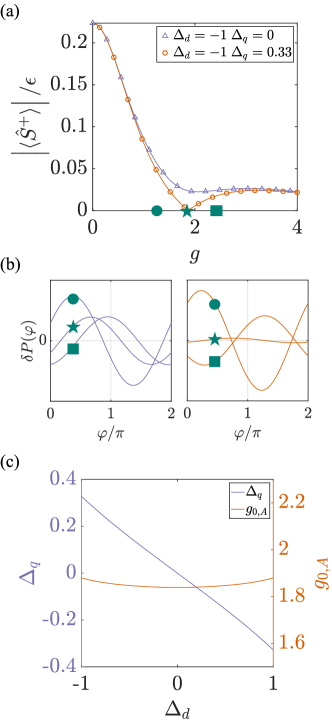
Figure 5: Phase-locking to a detuned drive. (a) $\lvert\langle\hat{S}^{+}\rangle\rvert/\epsilon$ for qubit $A$ versus the coupling strength $g$ for a detuned drive. The purple (orange) curves correspond to the case when qubit $B$ is resonant with (detuned from) qubit $A$. Markers (lines) are numerical (analytical) results. (b) The variation in the azimuthal phase distribution $\delta P(\varphi)$ [see Eq. (6)] for qubit $A$ when qubit $B$ is resonant with (left) and detuned from (right) qubit $A$, at the coupling strengths indicated in panel (a). (c) The value of the qubit-qubit detuning $\Delta_{q}$ at which the zero crossing is restored, and the corresponding coupling strength $g_{0,A}$, as a function of the drive detuning $\Delta_{d}$. Here, we choose $w_{A}=0.25,\gamma_{A}=0.75$ and $w_{B}=0.75,\gamma_{B}=0.25$.

These results provide a window into the internal dynamics of the composite two-qubit oscillator and demonstrate the role of system parameters such as bath temperatures, qubit-qubit interaction, and detunings in modifying the tendency of the constituent qubits to develop a preferred phase relative to the drive.

III.2 Synchronisation of the Composite System

We now shift from the viewpoint of the individual qubits and instead study the response of the two-qubit system as a whole. We study the synchronization of the composite oscillator to the weak external drive applied on qubit $A$ by using the synchronization measure $\Omega(\hat{\rho})$ given in Eq. (9). In the following, we will drop the $\hat{\rho}$ dependency while referring to this measure for notational convenience.

A key finding of our study is that qubit-qubit interactions can enhance the extent of synchronization to an external drive. We quantify the interaction-induced enhancement in synchronization via the ratio $R$ defined as the ratio of the values of $\Omega$ in the presence ($g\neq 0$) and absence ($g=0$) of qubit-qubit coupling, i.e.

$$R(g)=\frac{\Omega\rvert_{g}}{\Omega\rvert_{0}}.$$ (11)

In Fig. 6, we plot $R$ versus $g$ for two different sets of bath parameters for the two qubits. The purple curve demonstrates that, for appropriate choices of gain and loss rates, qubit-qubit interactions can significantly enhance the extent of synchronization in a composite oscillator. On the other hand, interactions can also strongly suppress synchronization, as evidenced by the sharp dip in the orange curve.

As discussed in Sec. II.4, the synchronization measure is sensitive to the magnitude of the individual coherences between pairs of levels. As a qualitative indicator of this sensitivity, in Fig. 6(b) we plot the quantities $\lvert\langle T|U\rangle\rvert$ and $\lvert\langle T|D\rangle\rvert$, corresponding to coherences in the collective spin basis, along the curves displayed in Fig. 6(a). The coherences $\langle S|U\rangle$ and $\langle S|D\rangle$ are respectively equal in magnitude to $\langle T|U\rangle$ and $\langle T|D\rangle$. We find that enhancement and suppression of the synchronization measure are associated with corresponding peaks and dips in the magnitude of coherences between pairs of levels in the collective spin picture, demonstrating that the synchronization measure captures the overall extent of coherence build-up in the system as a result of the drive.

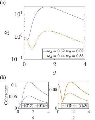
Figure 6: Enhancement and suppression of synchronisation of the composite two-qubit oscillator. The ratio $R$ [Eq. (11)] versus the coupling strength $g$ for two different sets of bath parameters, indicated by the $w_{A},w_{B}$ values in the legend. The total relaxation rate for each qubit is kept fixed at $\gamma_{A}+w_{A}=\gamma_{B}+w_{B}=1$. (b) Magnitude of coherences in the collective spin basis (see Sec. II.4), $\lvert\langle T|U\rangle\rvert$ and $\lvert\langle T|D\rangle\rvert$, along the curves shown in panel (a). Results are obtained numerically.

III.2.1 Synchronization enhancement: Dependence on gain and loss rates

The enhancement of synchronization as a result of qubit-qubit interaction depends on the parameters of the local thermal baths acting on each qubit. We once again first consider the situation when $\Delta_{d}=\Delta_{q}=0$. In Fig. 7(a) we plot $R_{\mathrm{max}}$, the value of $R$ maximized over the coupling strength $g$, as the gain rates for the two qubits (and consequently their temperatures) are varied. We observe that significant enhancement in synchronization occurs when the gain and loss rates for qubit $A$ are comparable. This can be understood by considering the limiting case of $w_{A}=\gamma_{A}$, which corresponds to an infinite temperature bath. For $g=0$, the steady state of qubit $A$ coupled to such a bath is the maximally mixed state, which does not develop any coherence under an external drive. However, coupling it to a second qubit with $w_{B}\neq\gamma_{B}$ takes the composite oscillator away from infinite temperature and leads to a build up of non-zero coherence in the system.

To see the effect of the qubit-qubit coupling in the region $w_{A}\sim\gamma_{A}$ more clearly, we compare the case of coupled and uncoupled ($g=0$) qubits in Fig. 7(b). We fix $w_{B}=0$ and plot $\Omega$ when it is maximized over $g$ ($\Omega_{\mathrm{max}}$), and for $g=0$ ($\Omega|_{0}$), as $w_{A}$ is varied. As $w_{A}\rightarrow\gamma_{A}$ ($w_{A}\rightarrow 0.5$ here), the coherence in the uncoupled system vanishes whereas it persists in the presence of interactions with qubit $B$. In fact, we find that for any non-zero temperature of qubit $A$, interactions with qubit $B$ with $w_{B}=0$ (zero temperature) lead to an enhancement in the synchronization measure, although this is most noticeable when $w_{A}\sim\gamma_{A}$.

We note that it is essential to keep in mind the actual value of the synchronization measure when interpreting enhancements in synchronization. For instance, as $w_{A}\rightarrow\gamma_{A}$, $R_{\mathrm{max}}\to\infty$. However, this result is an artefact of $\Omega|_{0}\to 0$ in this limit, whereas $\Omega_{\mathrm{max}}$ remains finite, but small. Nevertheless, even a small non-zero buildup of coherences can lead to observable effects in macroscopic systems with a large number of quantum units, as occurs in NMR systems [14].

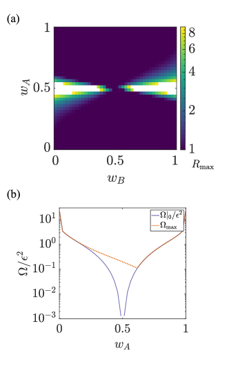
Figure 7: Effect of bath parameters on enhancement of synchronisation of the composite two-qubit oscillator. (a) Plot of $R_{\mathrm{max}}$, i.e. $R$ [Eq. (11)] maximized over coupling strength $g$, as $w_{A},w_{B}$ are scanned. The regions in white correspond to $R_{\mathrm{max}}>10$. (b) Synchronization measure $\Omega$ [Eq. (9)] versus $w_{A}$ for $w_{B}=0,\gamma_{B}=1$. The orange dashed (purple solid) line corresponds to $\Omega$ maximized over $g$ ($\Omega$ at $g=0$). In both panels, the total relaxation rate for each qubit is kept fixed at $\gamma_{A}+w_{A}=\gamma_{B}+w_{B}=1$. Results are obtained numerically.

III.2.2 Synchronization to a detuned drive

We now consider the synchronization of the composite oscillator to a detuned drive. In Fig. 8, we plot $R_{\mathrm{max}}$ as the detunings $\Delta_{d}$ and $\Delta_{q}$ are scanned for a fixed set of bath parameters. We find that the interaction-induced enhancement of synchronization can be even more pronounced for a detuned drive than in the resonant case, as evidenced by the larger values of $R_{\mathrm{max}}$ as $\lvert\Delta_{d}\rvert$ increases. Furthermore, for a detuned drive, the maximum enhancement occurs for a non-zero detuning of qubit $B$ from qubit $A$.

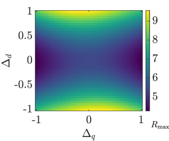
Figure 8: Synchronization of the composite two-qubit oscillator to a detuned drive. Plot of $R_{\mathrm{max}}$, i.e. $R$ [Eq. (11)] maximized over coupling strength $g$, as the drive and relative qubit detunings $\Delta_{d},\Delta_{q}$ are scanned. Here, we choose $w_{A}\approx 0.55,\gamma_{A}\approx 0.45$ and $w_{B}\approx 0.09,\gamma_{B}\approx 0.91$. Results are obtained numerically.

These results demonstrate how the overall buildup of coherences in a composite system under external driving can be strongly enhanced or suppressed by tuning the parameters of the constituent quantum units and the interactions between them. More broadly, the variety of quantum synchronizing behaviors observable in our minimal model exemplifies the potential to assemble quantum self-sustained oscillators using basic building blocks such as qubits, which can then be used as a playground to explore aspects and applications of quantum synchronization [23].

III.3 Experimental considerations

Motivated by practical considerations, we have studied the robustness of the features discussed above to qubit dephasing [see Eq. (15)] as well as stronger drive strengths such that $\epsilon/\Gamma\lesssim 1$. We find that both dephasing and stronger driving only lead to quantitative changes, e.g. in the location of the zero-crossing in Fig. 3(a) or the extent of synchronization enhancement in Fig. 6, but do not change the results qualitatively.

IV Proposal for Circuit QED Realization

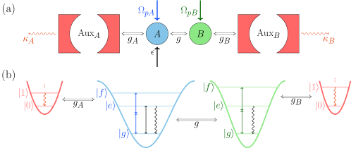
Figure 9: Circuit QED realization of a composite two-qubit oscillator. (a) Schematic showing two transmons $A$ and $B$ each coupled to a lossy auxiliary resonator as well as to each other, and driven using microwave fields. (b) Level diagram illustrating the working principle of the implementation.

In this section, we propose an implementation of our composite two-qubit oscillator model using artificial atoms and resonators made out of superconducting microwave circuits. This platform constitutes a favorable testbed to study synchronization for a number of reasons. These include the high degree of flexibility in the qubit connectivity, the ability to scale up the oscillator size if required, as well as the absence of certain undesirable effects such as motional heating, which often accompanies gain and loss channels in real atoms. In contrast to digital simulations of synchronizing systems on a superconducting quantum computer [15], here we propose an analog simulation approach to directly engineer the various Hamiltonian and dissipative processes of the oscillator, as discussed below.

Figure 9 shows a schematic of our proposed circuit QED implementation. The two qubits are encoded in the ground ($\ket{g}$) and first excited ($\ket{e}$) states of two tunable frequency transmons, labeled $A$ and $B$. While the loss channel, i.e. $\ket{e}\rightarrow\ket{g}$ decay, is intrinsic to each transmon, the gain channel, i.e. incoherent $\ket{g}\rightarrow\ket{e}$ jumps, need to be artificially engineered. Such a channel can be engineered by utilizing a lossy auxiliary resonator coupled to higher levels of the transmon [24, 25]. Specifically, for each transmon, a resonator with decay rate $\kappa_{j}$ ($j=A,B$) is coupled resonantly to its $\ket{e}\leftrightarrow\ket{f}$ transition. Exploiting the anharmonicity in the spacing of the transmon levels, two-photon $\ket{g}\rightarrow\ket{f}$ transitions can be driven resonantly by using appropriately detuned microwave ‘pump’ fields $\Omega_{pA},\Omega_{pB}$. Consequently, population in $\ket{g}$ is transferred to $\ket{f}$, which decays rapidly to $\ket{e}$ as a result of coupling to the lossy resonator. The net effect of this process is an incoherent transfer of population from $\ket{g}$ to $\ket{e}$, that realizes a gain channel. The qubit-qubit interaction is realized using a tunable coupler (not shown) that introduces spin-exchange interactions with variable coupling strength $g$. Finally, the external drive $\epsilon$ is realized as an additional microwave field applied on transmon $A$.

To verify the realization of a two-qubit oscillator using this system, we have identified appropriate values for the various system parameters and performed master equation simulations of the circuit QED model. In our modeling, we include the Hilbert space of the transmons as well as the auxiliary resonators, while we choose to model the coupler as a phenomenological tunable coupling term between the two transmons. Our choice is motivated by the multiple demonstrations of tunable couplers [26, 27, 28], making them a standard component in circuit QED systems. The details of the master equation simulations are discussed in Appendix E and the chosen parameter values are listed in Tables 1 and 2. These parameters are feasible with current technology. To experimentally measure the quantities discussed here, individual readout resonators can be coupled to each qubit (not shown), and the density matrix of the combined two-qubit system can be extracted by performing tomography using multiple single and two-qubit gates as done, e.g., in Ref. [29]. In the following, we focus on the simulation results, which demonstrate that our proposed system indeed operates as a composite two-qubit oscillator that can be used to explore the features discussed in Sec. III.

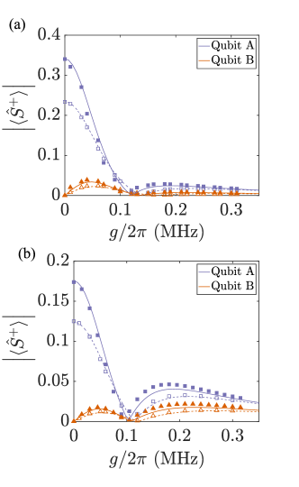
Figure 10: Phase locking of individual qubits in the circuit QED implementation. The two panels show $\lvert\langle\hat{S}^{+}\rangle\rvert$ for the two qubits with (a) $w_{A}/\gamma_{A}=0$, $w_{B}/\gamma_{B}\approx 3.2$ and (b) $w_{A}/\gamma_{A}\approx 0.27$ and $w_{B}/\gamma_{B}\approx 4.5$. The filled markers (solid lines) show the results from the circuit QED model (qubit model, discussed in Sec. III). The empty markers (dashed lines) are the corresponding results in the presence of an additional dephasing channel. Parameters for the simulations are presented in Appendix E.

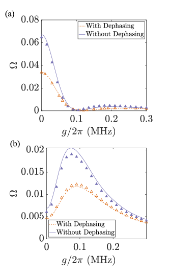
Figure 11: Synchronization of the composite oscillator in the circuit QED implementation. The two panels show the synchronization measure $\Omega$ [Eq. (9)] for (a) $w_{A}/\gamma_{A}\approx 0.27$, $w_{B}/\gamma_{B}\approx 4.5$ and (b) $w_{A}/\gamma_{A}\approx 0.71$, $w_{B}/\gamma_{B}\approx 0.28$. The solid markers (solid lines) show the results for the circuit QED model (qubit model, discussed in Sec. III). The empty markers and dashed lines are the corresponding results in the presence of an additional dephasing channel. Parameters for the simulations are presented in Appendix E.

In Fig. 10, we study the phase locking of the individual qubits to the external drive by plotting the coherence $\lvert\langle\hat{S}^{+}\rangle\rvert$ of the two qubits. The two panels correspond to two different sets of gain and loss rates for the two qubits. The results from the circuit QED model (markers) are in very good agreement with the expectations from the qubit model (lines) studied in Sec. III. In addition, we simulate the system in the presence of intrinsic transmon dephasing (empty markers and dashed lines) and find that it does not change the behavior qualitatively even when the dephasing rates are comparable to the relaxation rates $\gamma_{A},\gamma_{B}$. In Fig. 11, we compare the synchronization measure $\Omega$ obtained from the circuit QED model to the predictions from the qubit model and once again find excellent agreement for two different sets of gain and loss parameters. Our results suggest that features such as the zero crossing in the coherence of the individual qubits and the enhancement or suppression of quantum synchronization as a result of qubit-qubit interactions can be observed in a circuit QED experiment, and are robust against effects such as dephasing.

V Conclusion and outlook

We have introduced and studied a minimal model of a composite self-sustained oscillator consisting of two interacting qubits coupled to each other as well as to independent thermal baths. Such a model provides a first step towards engineering a wide variety of quantum synchronizing systems from basic units available on current quantum hardware. We studied the response of this system when a weak external drive is applied on one of the qubits from a ‘microscopic’ and a ‘macroscopic’ viewpoint. Specifically, we showed how the interplay of gain, loss and qubit-qubit interactions affects the phase locking of the constituent qubits to the drive as well as the tendency of the composite system, as a whole, to synchronize to the drive. Furthermore, we demonstrated the experimental feasibility of our model by proposing and analyzing a circuit QED implementation using transmons coupled to resonators as well as to each other.

Our study of the two-qubit oscillator provides insight into the behavior of the individual qubits as well as the system as a whole. We show that when the baths are inverted, i.e. when gain dominates loss for one qubit and loss dominates gain for the other, the phase locking of the individual qubits to the external drive undergoes an abrupt phase shift of $\pi$ as the qubit-qubit coupling strength increases. Remarkably, at the crossover points for either qubit, we observe a phase-locking blockade phenomenon: The off-diagonal element (coherence) of its reduced density matrix vanishes, restoring an azimuthal phase symmetry in the corresponding phase space distribution. We further study the tendency of the two-qubit oscillator, as a whole, to synchronize to the drive. We find that when the gain and loss rates for the driven qubit are comparable, interactions with the second qubit can significantly enhance the coherence induced in the system by the drive. On the other hand, we also find parameter regimes where qubit-qubit interactions can strongly suppress the synchronization of the system to the drive.

Our model naturally generalizes to higher dimensional spins, which may however be more challenging to implement in practice. In Appendix D, we study a two-qutrit oscillator and show that the behavior of this system is qualitatively similar to the two-qubit oscillator. An interesting observation in the qutrit system is the occurence of a zero crossing in the expectation values of higher-order spherical tensor operators at specific qutrit-qutrit coupling strengths, which can be interpreted as a generalized phase-locking blockade phenomenon.

Finally, let us note that our model and circuit QED proposal are complementary to, and build upon, previous studies of quantum synchronization with pairs of qubits in NMR platforms [14]. In contrast to these studies with an Ising interaction between the qubits, our model considers a spin-exchange type interaction between them. Furthermore, the qubit-qubit coupling strength and the individual qubit gain-to-loss ratios in our circuit QED proposal are tunable, allowing for control on the interactions and the local temperatures of each qubit. This enables the exploration of a wide variety of quantum synchronizing behaviors. More broadly, our proposal offers the potential to controllably scale up quantum self-sustained oscillators, and thereby experimentally probe the emergence of classical notions of synchronization from the underlying quantum system. For example, the properties of macroscopic synchronizing systems, such as superradiant lasers composed of several thousands to millions of atoms [30, 31, 32] and analogous systems [33, 34], can be understood as the response of a large collective dipole, that can be analyzed with semiclassical mean-field type theories. Theoretical analysis of scaled-up extensions of our model can be performed rigorously using recently introduced tools [35]. Our proposal may also find applications in studying complex thermal heat engines [36, 37] and exotic quantum heat engines, e.g., that operate between negative and positive temperature baths [38].

Appendix A Phase-locking metrics based on the $Q$ function

In Sec. III.1, we study the phase locking of the individual qubits using the off-diagonal element of the respective reduced density matrices. This metric was motivated in Sec. II.2 using the Husimi $Q$ function. This approach can be generalized to study the phase-locking of individual qudits in a two-qudit oscillator by expanding the $Q$ function in terms of spherical tensor operators. Specifically, the $Q$ function can be expressed as the sum [40, 41]

$$Q_{S}(\theta,\varphi)=\sum_{k=0}^{2S}\sum_{q=-k}^{k}c_{k,q}P_{k}^{q}(\cos\theta)e^{iq\varphi}\langle\hat{T}_{k}^{-q}\rangle,$$ (12)

where $P_{k}^{q}(\cos\theta)$ are associated Legendre polynomials, $\hat{T}_{k}^{q}$ are spherical tensor operators, $\langle\hat{O}\rangle=\mathrm{Tr}\{\hat{O}\hat{\rho}\}$ denotes the expectation value of an operator $\hat{O}$, and $c_{k,q}$ are weight factors given by

$$c_{k,q}=\sqrt{\frac{(2k+1)(k-q)!}{(k+q)!}}\frac{(2S)!}{\left[(2S-k)!(2S+k+1)!\right]^{1/2}}.$$ (13)

As a result, the phase-locking of individual qudits to an external drive that breaks the azimuthal phase symmetry can be studied by probing the expectation value of spherical tensor operators with $q$ different from zero.

In particular, for qubits and qutrits, the $Q$ function can be explicitly expressed as

$$Q_{\frac{1}{2},\hat{\rho}}(\theta,\varphi) = \frac{1}{\sqrt{2}}P_{0}^{0}\langle\hat{T}_{0}^{0}\rangle+\frac{1}{\sqrt{2}}P_{1}^{0}\langle\hat{T}_{1}^{0}\rangle+P_{1}^{1}\mathrm{Re}\left[\langle\hat{T}_{1}^{1}\rangle e^{-i\varphi}\right],$$

$$Q_{1,\hat{\rho}}(\theta,\varphi) = \frac{1}{\sqrt{3}}P_{0}^{0}\langle\hat{T}_{0}^{0}\rangle+\frac{1}{\sqrt{2}}P_{1}^{0}\langle\hat{T}_{1}^{0}\rangle+\frac{1}{\sqrt{6}}P_{2}^{0}\langle\hat{T}_{2}^{0}\rangle$$ (14)

$$+\mathrm{Re}\left[\left\{P_{1}^{1}\langle\hat{T}_{1}^{1}\rangle+\frac{1}{3}P_{2}^{1}\langle\hat{T}_{2}^{1}\rangle\right\}e^{-i\varphi}+\frac{1}{6}P_{2}^{2}\langle\hat{T}_{2}^{2}\rangle e^{-2i\varphi}\right],$$

where we have used $P_{k}^{q}\equiv P_{k}^{q}(\cos\theta)$ for compactness and expressed the $Q$ function using only the $q\geq 0$ terms. Writing the spherical tensor operators in $Q_{1/2}$ in terms of spin operators, we obtain Eq. (LABEL:eqn:q_half_spin). In the case of spin-$1$, two multipoles $\hat{T}_{1}^{1},\hat{T}_{2}^{1}$ contribute to the first harmonic in $\varphi$, while $\hat{T}_{2}^{2}$ gives rise to a second harmonic. We study these quantities in the context of a two-qutrit oscillator in Appendix D.

Appendix B Partially coherent candidate limit cycle states

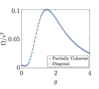
Figure 12: Synchronisation measure ($\Omega/\epsilon^{2}$) of the composite two-qubit oscillator computed using the diagonal limit cycle state and an optimization over the partially-coherent limit cycle states. Here, we choose $w_{A}\approx 0.55,\gamma_{A}\approx 0.45$ and $w_{B}\approx 0.09,\gamma_{B}\approx 0.91$. Results are obtained numerically.

In Sec. II.3, we describe a metric [Eq. (9)] for studying the synchronization of the two-qubit oscillator, which we use to obtain the results in Sec. III.2. This metric is obtained considering a family of limit cycle states $\Sigma$ that is diagonal in the eigenbasis $\{\ket{\lambda_{j}}\}$ of the undriven steady state $\hat{\rho}_{u}$. We note that the $\{\ket{\lambda_{j}}\}$ are not the eigenstates $\{\ket{E_{j}}\}$ of the undriven Hamiltonian, i.e. Eq. (1) with $\epsilon=0$. Under such circumstances, Ref. [16] proposes to optimize over a more general family of limit cycle states that allow for partial coherence in the $\{\ket{E_{j}}\}$ basis, such that the resulting family of states respects the structure of $\hat{\rho}_{u}$ expressed in this basis. Here, we demonstrate that in our model and for weak driving, the metric (9) essentially coincides with the measure obtained by optimization over such partially coherent limit cycle states.

We first note that, in our model, both sets, $\{\ket{\lambda_{j}}\}$ and $\{\ket{E_{j}}\}$, are eigenstates of the operator $\hat{S}^{z}=\hat{S}^{z}_{A}+\hat{S}^{z}_{B}$. As a result, $\hat{\rho}_{u}$ can be written in a block-diagonal form in the basis $\{\ket{E_{j}}\}$, with each block corresponding to a fixed number of total excitations. Under such a situation, $\Sigma$ must be chosen as a set of partially-coherent candidate limit cycle states that account for the intrinsic coherences in each block that are not established by the drive. On the other hand, the matrix elements of the external drive ($\epsilon$ term in Eq. (1)) are block off-diagonal in $\{\ket{E_{j}}\}$. In other words, $\hat{\rho}_{u}$ respects a global $U(1)$ symmetry, i.e. it is invariant under unitary transformations of the form $\hat{U}(\varphi)=e^{-i\varphi\hat{S}^{z}}$, while the weak drive, to leading order, only introduces coherences between different blocks associated with this symmetry. As a result, for weak driving, we expect the synchronization measure computed by choosing $\Sigma$ as the set of states diagonal in $\{\lambda_{j}\}$ (as done in the main text) to coincide with the measure computed using the set of states with partial coherence (as described above) in the $\{\ket{E_{j}}\}$ basis.

In Fig. 12, we demonstrate the excellent agreement between the two approaches. We compute the synchronization measure using partially-coherent candidate limit cycle states via numerical optimization of the limit cycle after imposing the block-diagonal structure in the $\{\ket{E_{j}}\}$ basis. Indeed, we find that the optimized partially coherent limit cycle state coincides with $\hat{\rho}_{\mathrm{diag}}$. In the main text, we choose to work with the metric based on diagonal limit cycle states as they are conceptually simpler and more intuitive.

Appendix C Phase-locking of individual qubits: Analytical solution

In this appendix, we outline our procedure to obtain analytical expressions for the phase locking measures $\lvert\langle\hat{S}_{j}^{+}\rangle\rvert,j=A,B$, using which we rigorously establish the presence of zero-crossing points in Sec. III.

The master equation for the system, including dephasing noise on the qudits for a general treatment, is

$$\frac{d\hat{\rho}}{dt}=-i\left[\hat{H}_{\mathrm{tot}},\hat{\rho}\right]+\sum_{j={A,B}}\mathfrak{D}[\sqrt{w_{j}}\hat{S}_{j}^{+}]\hat{\rho}$$ (15)

$$+\sum_{j={A,B}}\mathfrak{D}[\sqrt{\gamma_{j}}\hat{S}_{j}^{-}]\hat{\rho}+\sum_{j={A,B}}\mathfrak{D}[\sqrt{2\gamma_{\phi}}\hat{S}_{j}^{z}]\hat{\rho},$$

where $\hat{H}_{\mathrm{tot}}$ is given by Eq. (1). We treat the drive as a perturbation and expand all observables in orders of $\epsilon$ as

$$\braket{\hat{O}}=\braket{\hat{O}}_{0}+\epsilon\braket{\hat{O}}_{1}+\mathcal{O}(\epsilon^{2}).$$ (16)

At zeroth order in $\epsilon$, the master equation is $U(1)$ symmetric, i.e. it is invariant under the transformation $\hat{S}_{A(B)}^{\pm}\rightarrow\hat{S}_{A(B)}^{\pm}e^{\pm i\varphi}$. As a result, only observables that are invariant under this symmetry are non-zero. There are four such quantities, corresponding (at zeroth order) to $\braket{\hat{S}_{A}^{z}}_{0},\braket{\hat{S}_{B}^{z}}_{0},\braket{\hat{S}_{A}^{z}\hat{S}_{B}^{z}}_{0},\braket{\hat{S}_{A}^{+}\hat{S}_{B}^{-}}_{0}$. Their equations of motion constitute a set of linear equations given by

$$\mathrm{Re}\left\{ig\braket{\hat{S}_{A}^{-}\hat{S}_{B}^{+}}_{0}\right\}-\Gamma_{A}\braket{\hat{S}_{A}^{z}}_{0}=-\frac{w_{A}-\gamma_{A}}{2}$$ (17)

$$\mathrm{Re}\left\{ig\braket{\hat{S}_{A}^{+}\hat{S}_{B}^{-}}_{0}\right\}-\Gamma_{B}\braket{\hat{S}_{B}^{z}}_{0}=-\frac{w_{B}-\gamma_{B}}{2}$$

$$\frac{w_{B}-\gamma_{B}}{2}\braket{\hat{S}_{A}^{z}}_{0}+\frac{w_{A}-\gamma_{A}}{2}\braket{\hat{S}_{B}^{z}}_{0}-(\Gamma_{A}+\Gamma_{B})\braket{\hat{S}_{A}^{z}\hat{S}_{B}^{z}}_{0}=0$$

$$i\frac{g}{2}\left(\braket{\hat{S}_{B}^{z}}_{0}-\braket{\hat{S}_{A}^{z}}_{0}\right)-\frac{\Gamma_{A}+\Gamma_{B}+4\gamma_{\phi}}{2}\braket{\hat{S}_{A}^{+}\hat{S}_{B}^{-}}_{0}-i\Delta_{q}\braket{\hat{S}_{A}^{+}\hat{S}_{B}^{-}}_{0}=0,$$

where $\Gamma_{A(B)}=w_{A(B)}+\gamma_{A(B)}$. At first order in $\epsilon$, observables with broken $U(1)$ symmetry acquire a non-zero value. In particular, their equations of motion are ‘sourced’ by the zeroth order $U(1)$ symmetric observables as given below:

$$-ig\braket{\hat{S}_{A}^{z}\hat{S}_{B}^{+}}_{1}-\frac{\Gamma_{A}+2\gamma_{\phi}}{2}\braket{\hat{S}_{A}^{+}}_{1}+i\Delta_{d}\braket{\hat{S}_{A}^{+}}_{1}=i\braket{\hat{S}_{A}^{z}}_{0}$$ (18)

$$-ig\braket{\hat{S}_{A}^{+}\hat{S}_{B}^{z}}_{1}-\frac{\Gamma_{B}+2\gamma_{\phi}}{2}\braket{\hat{S}_{B}^{+}}_{1}+i(\Delta_{d}+\Delta_{q})\braket{\hat{S}_{B}^{+}}_{1}=0$$

$$-i\frac{g}{4}\braket{\hat{S}_{B}^{+}}_{1}-\frac{\Gamma_{A}+2\gamma_{\phi}}{2}\braket{\hat{S}_{A}^{+}\hat{S}_{B}^{z}}_{1}+\frac{w_{B}-\gamma_{B}}{2}\braket{\hat{S}_{A}^{+}}_{1}-\Gamma_{B}\braket{\hat{S}_{A}^{+}\hat{S}_{B}^{z}}_{1}+i\Delta_{d}\braket{\hat{S}_{A}^{+}\hat{S}_{B}^{z}}_{1}=i\braket{\hat{S}_{A}^{z}\hat{S}_{B}^{z}}_{0}$$

$$-i\frac{g}{4}\braket{\hat{S}_{A}^{+}}_{1}-\frac{\Gamma_{B}+2\gamma_{\phi}}{2}\braket{\hat{S}_{A}^{z}\hat{S}_{B}^{+}}_{1}+\frac{w_{A}-\gamma_{A}}{2}\braket{\hat{S}_{B}^{+}}_{1}-\Gamma_{A}\braket{\hat{S}_{A}^{z}\hat{S}_{B}^{+}}_{1}+i(\Delta_{d}+\Delta_{q})\braket{\hat{S}_{A}^{z}\hat{S}_{B}^{+}}_{1}=-\frac{i}{2}\braket{\hat{S}_{A}^{-}\hat{S}_{B}^{+}}_{0}$$

$$-\frac{\Gamma_{A}+\Gamma_{B}+4\gamma_{\phi}}{2}\braket{\hat{S}_{A}^{+}\hat{S}_{B}^{+}}_{1}+i(2\Delta_{d}+\Delta_{q})\braket{\hat{S}_{A}^{+}\hat{S}_{B}^{+}}_{1}=0.$$

Solving these equations, we arrive at analytic expressions for $\langle\hat{S}_{A}^{+}\rangle,\langle\hat{S}_{B}^{+}\rangle$. However, the general form of these expressions are not compact and hence we do not reproduce them here.

Appendix D Two-qutrit oscillator

Our model can be generalised to explore higher dimensional spin systems. In this appendix, we briefly study an oscillator composed of two interacting qutrits that are each coupled to separate thermal baths.

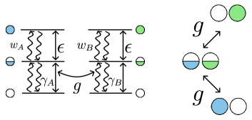
Figure 13: Energy level diagram for the composite two-qutrit oscillator, showing the gain and damping channels and the exchange interaction of the qutrits. The right panel illustrates the exchange interactions. The white, half-colored and colored circles respectively represent the $m=-1,0,1$ states of the two qutrits.

D.1 Phase Locking of Individual Qutrits

We study the phase locking of the constituent qutrits to an external drive applied on one of them using the spherical tensors framework described in Appendix A. Accordingly, in Fig. 14(a), we plot the quantities $\lvert\braket{\hat{T}_{1}^{1}}\rvert,\lvert\braket{\hat{T}_{2}^{1}}\rvert$ and $\lvert\braket{\hat{T}_{2}^{2}}\rvert$ for qutrit $A$ as a function of the qutrit-qutrit coupling strength and for a fixed set of gain and loss rates for each qutrit. Interestingly, we observe that each of the three quantities undergoes a zero crossing at different coupling strengths. This observation can be interpreted as a generalized phase-locking blockade effect, where the expectation values of specific spherical tensor multipoles vanish as a result of destructive interference from the coupling to the second qutrit.

D.2 Synchronisation of the Composite Two-Qutrit oscillator

In Fig. 15, we plot the quantity $R$, defined in Eq. (11), as a function of the qutrit-qutrit coupling strength for two different sets of gain and loss rates for the qutrits. These curves demonstrate that interactions between the two qutrits can lead to significant enhancement or suppression of synchronization in different parameter regimes, similar to the case of the two-qubit oscillator discussed in the main text.

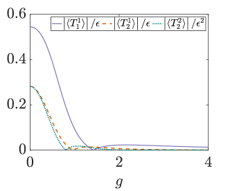
Figure 14: Expectation values of spherical tensor operators for qutrit $A$ versus the qutrit-qutrit coupling strength $g$. Here, we choose $w_{A}=0.25,\gamma_{A}=0.75$ and $w_{B}=0.75,\gamma_{B}=0.25$, while fixing $w_{A}+\gamma_{A}=w_{B}+\gamma_{B}=1$. Results are obtained numerically.

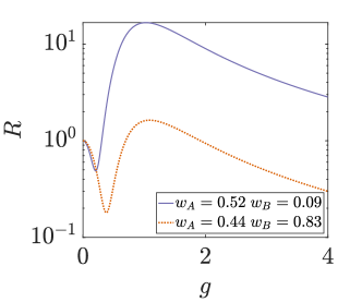
Figure 15: Enhancement and suppression of synchronisation of the composite two-qutrit oscillator. The ratio $R$ [Eq. (11)] versus the coupling strength $g$ for the two-qutrit oscillator and for two different sets of bath parameters, indicated by the $w_{A},w_{B}$ values in the legend. Results are obtained numerically.

Appendix E Simulations of Proposed cQED Realization

In this appendix, we describe the master equation, parameter values and factors considered in choosing these values, for the results presented in Sec. IV.

The master equation simulation is performed using QuTiP [39] for the system depicted in Fig. 9. We include $3$ levels for each transmon and auxiliary resonator for the simulation and choose to work in a frame that is rotating at the frequencies $\omega_{pA},\omega_{pB}$ of the two-photon ‘pump’ fields, which are denoted by their Rabi frequencies $\Omega_{p_{A}},\Omega_{p_{B}}$ in Fig. 9. The Hamiltonian in such a frame is given by

$$\hat{H}_{\mathrm{cQED}} =\sum_{j={A,B}}(\omega_{qj}-\omega_{pj})\hat{b}^{\dagger}_{j}\hat{b}_{j}+\sum_{j={A,B}}\frac{\alpha_{j}}{2}(\hat{b}^{\dagger}_{j}\hat{b}_{j}-1)\hat{b}^{\dagger}_{j}\hat{b}_{j}$$ (19)

$$+\sum_{j={A,B}}(\omega_{aj}-\omega_{pj})\hat{a}^{\dagger}_{j}\hat{a}_{j}$$

$$+\sum_{j={A,B}}g_{j}(\hat{a}_{j}\hat{b}^{\dagger}_{j}+\hat{a}^{\dagger}_{j}\hat{b}_{j})$$

$$+g(\hat{b}^{\dagger}_{A}\hat{b}_{B}e^{i(\omega_{pA}-\omega_{pB})t}+\mathrm{h.c.})$$

$$+\sum_{j={A,B}}\Omega_{pj}(\hat{b}^{\dagger}_{j}+\hat{b}_{j})$$

$$+\epsilon(\hat{b}_{A}e^{-i(\omega_{pA}-\omega_{qA})t}+\mathrm{h.c.}).$$

Here, $\hat{a}_{j},\hat{a}_{j}^{\dagger}$ and $\hat{b}_{j},\hat{b}_{j}^{\dagger}$, $j=A,B$, are the ladder operators for the auxiliary resonators and the transmons respectively. We note that the coupling and drive strengths in this model differ by a factor of two in comparison to the spin model Eq. (1). The first two lines in Eq. (19) describe the free Hamiltonian of the transmons and the auxiliary resonators. The third line describes the coupling between the transmons and their respective auxiliary resonators, the fourth line the coupling between the two transmons, the fifth line the two-photon pump on the transmons, and the last line describes the external drive on transmon $A$. The master equation for the full system is given by

$$\frac{d\hat{\rho}}{dt}=-i\left[\hat{H}_{\mathrm{cQED}},\hat{\rho}\right]+\sum_{j={A,B}}\mathfrak{D}[\sqrt{\kappa_{j}}\hat{a}_{j}]\hat{\rho}$$ (20)

$$+\sum_{j={A,B}}\mathfrak{D}[\sqrt{\gamma_{0,j}}\hat{b}_{j}]\hat{\rho}+\sum_{j={A,B}}\mathfrak{D}[\sqrt{\gamma_{\phi j}}\hat{b}^{\dagger}_{j}\hat{b}_{j}]\hat{\rho}.$$

Here, $\kappa_{j},\gamma_{0,j}$ describe the decay rates of the resonators and the transmons while $\gamma_{\phi_{j}}$ describe additional dephasing of the transmons. The values of the parameters entering Eq. (19) and Eq. (20) are given in Tables 1 and 2. These values are experimentally achievable with current technology.

A number of factors must be carefully considered in choosing parameters for the cQED model, and in order to match its results with the two-qubit oscillator model discussed in Sec. III. The off-resonant coupling of the $\ket{g}\leftrightarrow\ket{e}$ transition to the auxiliary resonator leads to an additional Purcell decay besides the intrinsic decay channels. The total decay rate $\gamma_{j}$ and the effective repump rate $w_{j}$ of each qubit, that are reported in Figs. 10 and 11, are extracted by decoupling the transmons ($g=0$) and fitting the relaxation profiles of the population from an initial state. While the $\ket{g}\leftrightarrow\ket{e}$ transitions of the two transmons must be near-resonance, the corresponding $\ket{e}\leftrightarrow\ket{f}$ transitions must be mismatched in frequency, which will require different anharmonicities for the two transmons. The frequency mismatch ensures that the $\ket{f}\rightarrow\ket{e}$ decay of, say transmon $A$, does not occur through the auxiliary resonator of transmon $B$ or vice versa, by virtue of their coupling. Furthermore, the strength $\epsilon$ of the weak drive cannot be made arbitrarily small since its effects must be discernible in the presence of experimental limitations and residual coherences arising from the pump fields.

Parameter	Symbol	Value
frequency of qubit A*(B*)	$\omega_{qA}(\omega_{qB})/2\pi$	5 GHz
frequency of aux A(B)	$\omega_{aA}(\omega_{aB})/2\pi$	4.6 GHz
anharmonicity of qubit $A$	$\alpha_{A}/2\pi$	400 MHz
anharmonicity of qubit $B$	$\alpha_{B}/2\pi$	500 MHz
qubit-qubit coupling	$g_{AB}/2\pi$	0 - 350 kHz
qubit $A$ - aux $A$ coupling	$g_{A}/2\pi$	8 MHz
qubit $B$ - aux $B$ coupling	$g_{B}/2\pi$	4 MHz
frequency of qubit $A$ pump	$\omega_{pA}/2\pi$	4.8 GHz
frequency of qubit $B$ pump	$\omega_{pB}/2\pi$	4.75 GHz
decay rate of aux $A$($B$)	$\kappa_{A}(\kappa_{B})/2\pi$	60 MHz
decay rate of qubit $A$($B$)	$\gamma_{0,A}(\gamma_{0,B})/2\pi$	53 kHz
dephasing rate of qubit $A$($B$)	$\gamma_{\phi A}(\gamma_{\phi B})/2\pi$	53 kHz

Table 1: Model parameters. For the quantities marked with a *, the values reported in this Table are approximate and need to be adjusted according to the detunings given in Table 2.

Symbol	Fig 10(a)	Fig 10(b) and Fig 11(a)	Fig 11(b)
$\epsilon/2\pi$	20 kHz	20 kHz	40 kHz
$\Omega_{pA}/2\pi$	0.0 MHz	5.5 MHz	7 MHz
$\Omega_{pB}/2\pi$	8.0 MHz	9.0 MHz	4.1 MHz
$\Delta_{A}/2\pi$	160 kHz	763.3 kHz	1135 kHz
$\Delta_{B}/2\pi$	1013.72 kHz	1230 kHz	300 kHz

Table 2: Parameters for different figures. $\Omega_{pA},\Omega_{pB}$ are the Rabi frequencies of the two-photon pump on qubits $A,B$ respectively. $\Delta_{A}$ and $\Delta_{B}$ are corrections in the qubit frequency due to the two-photon pump and the auxiliary resonator, such that the shifted frequency of the qubit is given by $\omega_{qj}+\Delta_{j},j=A,B$.

A further, important factor is that the auxiliary resonators and the two-photon pumps introduce shifts to the $\ket{g}\leftrightarrow\ket{e}$ transition frequency of both transmons, which must be compensated by appropriately tuning their frequencies. The dispersive shift of the $\ket{g}\leftrightarrow\ket{e}$ transition frequency arising from the auxiliary resonator is given by $g_{j}^{2}/(\omega_{qj}-\omega_{aj})$. The shift due to the two-photon pump was calculated by considering the Hamiltonian for the pump acting on the lowest three levels of the transmon. Because of the coupling to the auxiliary resonator, the decay in the third level, given by $\gamma_{f}=4g^{2}/\kappa$ [24], is also included in the Hamiltonian, which, in a frame rotating at the pump frequency takes the form

$$H=\begin{bmatrix}0&\Omega_{p}&0\\ \Omega_{p}&\alpha/2&\sqrt{2}\Omega_{p}\\ 0&\sqrt{2}\Omega_{p}&-i\gamma_{f}\end{bmatrix}$$ (21)

where $\Omega_{p}$ is the two-photon pump strength. The shifted $\ket{g}\leftrightarrow\ket{e}$ transition frequency is then obtained by diagonalizing this Hamiltonian. The net corrections to the transmon frequencies arising from the auxiliary resonators and the two-photon pumps are listed in Table 2.

References

- Pikovsky et al. [2001] A. Pikovsky, M. Rosenblum, and J. Kurths, Synchronization: A universal concept in nonlinear sciences, Self 2, 3 (2001).
- Lee and Sadeghpour [2013] T. E. Lee and H. Sadeghpour, Quantum synchronization of quantum van der pol oscillators with trapped ions, Physical review letters 111, 234101 (2013).
- Walter et al. [2014] S. Walter, A. Nunnenkamp, and C. Bruder, Quantum synchronization of a driven self-sustained oscillator, Physical review letters 112, 094102 (2014).
- Lee et al. [2014] T. E. Lee, C.-K. Chan, and S. Wang, Entanglement tongue and quantum synchronization of disordered oscillators, Physical Review E 89, 022913 (2014).
- Sonar et al. [2018] S. Sonar, M. Hajdušek, M. Mukherjee, R. Fazio, V. Vedral, S. Vinjanampathy, and L.-C. Kwek, Squeezing enhances quantum synchronization, Physical review letters 120, 163601 (2018).
- Roulet and Bruder [2018a] A. Roulet and C. Bruder, Quantum synchronization and entanglement generation, Physical review letters 121, 063601 (2018a).
- Roulet and Bruder [2018b] A. Roulet and C. Bruder, Synchronizing the smallest possible system, Physical review letters 121, 053601 (2018b).
- Koppenhöfer and Roulet [2019] M. Koppenhöfer and A. Roulet, Optimal synchronization deep in the quantum regime: Resource and fundamental limit, Phys. Rev. A 99, 043804 (2019).
- Tan et al. [2022] R. Tan, C. Bruder, and M. Koppenhöfer, Half-integer vs. integer effects in quantum synchronization of spin systems, Quantum 6, 885 (2022).
- Lörch et al. [2017] N. Lörch, S. E. Nigg, A. Nunnenkamp, R. P. Tiwari, and C. Bruder, Quantum synchronization blockade: Energy quantization hinders synchronization of identical oscillators, Physical Review Letters 118, 243602 (2017).
- Nigg [2018] S. E. Nigg, Observing quantum synchronization blockade in circuit quantum electrodynamics, Physical Review A 97, 013811 (2018).
- Solanki et al. [2022] P. Solanki, F. M. Mehdi, M. Hajdušek, and S. Vinjanampathy, Symmetries and synchronization blockade, arXiv preprint arXiv:2212.09388 (2022).
- Laskar et al. [2020] A. W. Laskar, P. Adhikary, S. Mondal, P. Katiyar, S. Vinjanampathy, and S. Ghosh, Observation of quantum phase synchronization in spin-1 atoms, Physical review letters 125, 013601 (2020).
- Krithika et al. [2022] V. Krithika, P. Solanki, S. Vinjanampathy, and T. Mahesh, Observation of quantum phase synchronization in a nuclear-spin system, Physical Review A 105, 062206 (2022).
- Koppenhöfer et al. [2020] M. Koppenhöfer, C. Bruder, and A. Roulet, Quantum synchronization on the ibm q system, Physical Review Research 2, 023026 (2020).
- Jaseem et al. [2020a] N. Jaseem, M. Hajdušek, P. Solanki, L.-C. Kwek, R. Fazio, and S. Vinjanampathy, Generalized measure of quantum synchronization, Physical Review Research 2, 043287 (2020a).
- Ameri et al. [2015] V. Ameri, M. Eghbali-Arani, A. Mari, A. Farace, F. Kheirandish, V. Giovannetti, and R. Fazio, Mutual information as an order parameter for quantum synchronization, Phys. Rev. A 91, 012301 (2015).
- Shen et al. [2023] Y. Shen, W.-K. Mok, C. Noh, A. Q. Liu, L.-C. Kwek, W. Fan, and A. Chia, Quantum synchronization effects induced by strong nonlinearities, arXiv preprint arXiv:2301.02948 (2023).
- Buča et al. [2022] B. Buča, C. Booker, and D. Jaksch, Algebraic theory of quantum synchronization and limit cycles under dissipation, SciPost Phys. 12, 097 (2022).
- Tindall et al. [2020] J. Tindall, C. S. Muñoz, B. Buča, and D. Jaksch, Quantum synchronisation enabled by dynamical symmetries and dissipation, New Journal of Physics 22, 013026 (2020).
- Note [1] We have omitted a normalization factor [7] for simplicity. More generally, the function for a spin- system can also be defined with respect to coherent states [12, 36, 37], but it is not required for our discussion here.
- Lee Loh and Kim [2015] Y. Lee Loh and M. Kim, Visualizing spin states using the spin coherent state representation, American Journal of Physics 83, 30 (2015).
- Jaseem et al. [2020b] N. Jaseem, M. Hajdušek, V. Vedral, R. Fazio, L.-C. Kwek, and S. Vinjanampathy, Quantum synchronization in nanoscale heat engines, Phys. Rev. E 101, 020201 (2020b).
- Sokolova et al. [2021] A. A. Sokolova, G. P. Fedorov, E. V. Il’ichev, and O. V. Astafiev, Single-atom maser with an engineered circuit for population inversion, Phys. Rev. A 103, 013718 (2021).
- Sokolova et al. [2023] A. A. Sokolova, D. A. Kalacheva, G. P. Fedorov, and O. V. Astafiev, Overcoming photon blockade in a circuit-qed single-atom maser with engineered metastability and strong coupling, Phys. Rev. A 107, L031701 (2023).
- Li et al. [2020] X. Li, T. Cai, H. Yan, Z. Wang, X. Pan, Y. Ma, W. Cai, J. Han, Z. Hua, X. Han, et al., Tunable coupler for realizing a controlled-phase gate with dynamically decoupled regime in a superconducting circuit, Physical Review Applied 14, 024070 (2020).
- Yan et al. [2018] F. Yan, P. Krantz, Y. Sung, M. Kjaergaard, D. L. Campbell, T. P. Orlando, S. Gustavsson, and W. D. Oliver, Tunable coupling scheme for implementing high-fidelity two-qubit gates, Physical Review Applied 10, 054062 (2018).
- Sung et al. [2021] Y. Sung, L. Ding, J. Braumüller, A. Vepsäläinen, B. Kannan, M. Kjaergaard, A. Greene, G. O. Samach, C. McNally, D. Kim, A. Melville, B. M. Niedzielski, M. E. Schwartz, J. L. Yoder, T. P. Orlando, S. Gustavsson, and W. D. Oliver, Realization of high-fidelity cz and -free iswap gates with a tunable coupler, Phys. Rev. X 11, 021058 (2021).
- Li et al. [2017] M. Li, G. Xue, X. Tan, Q. Liu, K. Dai, K. Zhang, H. Yu, and Y. Yu, Two-qubit state tomography with ensemble average in coupled superconducting qubits, Applied Physics Letters 110, 10.1063/1.4979652 (2017), 132602.
- Bohnet et al. [2012] J. G. Bohnet, Z. Chen, J. M. Weiner, D. Meiser, M. J. Holland, and J. K. Thompson, A steady-state superradiant laser with less than one intracavity photon, Nature 484, 78 (2012).
- Xu et al. [2014] M. Xu, D. A. Tieri, E. Fine, J. K. Thompson, and M. J. Holland, Synchronization of two ensembles of atoms, Physical review letters 113, 154101 (2014).
- Weiner et al. [2017] J. M. Weiner, K. C. Cox, J. G. Bohnet, and J. K. Thompson, Phase synchronization inside a superradiant laser, Phys. Rev. A 95, 033808 (2017).
- Zhu et al. [2015] B. Zhu, J. Schachenmayer, M. Xu, F. Herrera, J. G. Restrepo, M. J. Holland, and A. M. Rey, Synchronization of interacting quantum dipoles, New Journal of Physics 17, 083063 (2015).
- Shankar et al. [2017] A. Shankar, J. Cooper, J. G. Bohnet, J. J. Bollinger, and M. Holland, Steady-state spin synchronization through the collective motion of trapped ions, Phys. Rev. A 95, 033423 (2017).
- Landa and Misguich [2023] H. Landa and G. Misguich, Nonlocal correlations in noisy multiqubit systems simulated using matrix product operators, SciPost Phys. Core 6, 037 (2023).
- Murtadho et al. [2023a] T. Murtadho, S. Vinjanampathy, and J. Thingna, Cooperation and competition in synchronous open quantum systems (2023a), arXiv:2301.04322 [quant-ph] .
- Murtadho et al. [2023b] T. Murtadho, J. Thingna, and S. Vinjanampathy, Synchronization lower bounds the efficiency of near-degenerate thermal machines (2023b), arXiv:2301.04323 [quant-ph] .
- Bera et al. [2023] M. L. Bera, T. Pandit, K. Chatterjee, V. Singh, M. Lewenstein, U. Bhattacharya, and M. N. Bera, Steady-state quantum thermodynamics with synthetic negative temperatures (2023), arXiv:2305.01215 [quant-ph] .
- Johansson et al. [2012] J. R. Johansson, P. D. Nation, and F. Nori, QuTiP: An open-source Python framework for the dynamics of open quantum systems, Computer Physics Communications 183, 1760 (2012).
- Dowling et al. [1994] J. P. Dowling, G. S. Agarwal, and W. P. Schleich, Wigner distribution of a general angular-momentum state: Applications to a collection of two-level atoms, Physical Review A 49, 4101 (1994).
- Agarwal [1981] G. S. Agarwal, Relation between atomic coherent-state representation, state multipoles, and generalized phase-space distributions, Physical Review A 24, 2889 (1981).