Synthesising Recursive Functions for First-Order Model Counting:
Challenges, Progress, and Conjectures

Abstract

First-order model counting (FOMC) is a computational problem that asks to count the models of a sentence in finite-domain first-order logic. In this paper, we argue that the capabilities of FOMC algorithms to date are limited by their inability to express many types of recursive computations. To enable such computations, we relax the restrictions that typically accompany domain recursion and generalise the circuits used to express a solution to an FOMC problem to directed graphs that may contain cycles. To this end, we adapt the most well-established (weighted) FOMC algorithm ForcLift to work with such graphs and introduce new compilation rules that can create cycle-inducing edges that encode recursive function calls. These improvements allow the algorithm to find efficient solutions to counting problems that were previously beyond its reach, including those that cannot be solved efficiently by any other exact FOMC algorithm. We end with a few conjectures on what classes of instances could be domain-liftable as a result.

1 Introduction

(a) ForcLift compiles $\phi$ into a circuit $C_{\phi}$. The domain sizes are then used to propagate values through $C_{\phi}$, computing the model count.

(b) Crane compiles $\phi$ into a graph $G_{\phi}$ and then converts $G_{\phi}$ into a collection of functions $\mathcal{F}_{\phi}$. In some cases, these functions can benefit from algebraic simplification. If some functions are defined recursively, base cases need to be established. One can then compute the model count of $\phi$ by running the main function in $\mathcal{F}^{\prime}_{\phi}$ with domain sizes as arguments.

Figure 1: A comparison of how ForcLift and Crane can be used to compute the model count of a formula $\phi$

First-order model counting (FOMC) is the problem of computing the number of models of a sentence in first-order logic given the size(s) of its domain(s) (?). Symmetric weighted FOMC (WFOMC) extends FOMC with (pairs of) weights on predicates and asks for a weighted sum across all models instead. By fixing the sizes of the domains, a WFOMC instance can be rewritten as an instance of (propositional) weighted model counting (?). WFOMC emerged as the dominant approach to lifted (probabilistic) inference. Lifted inference techniques exploit symmetries in probabilistic models by reasoning about sets rather than individuals (?). By doing so, many instances become solvable in polynomial time (?). The development of lifted inference algorithms coincided with work on probabilistic relational models that combine the syntactic power of first-order logic with probabilistic models such as Bayesian and Markov networks, allowing for a more relational view of uncertainty modelling (?; ?; ?). Lifted inference techniques for probabilistic databases have also been inspired by WFOMC (?; ?). While WFOMC has received more attention in the literature, FOMC is an interesting problem in and of itself because of its connections to finite model theory (?) and applications in enumerative combinatorics (?).

Traditionally in computational complexity theory, a problem is tractable if it can be solved in time polynomial in the instance size. The equivalent notion in (W)FOMC is liftability. A (W)FOMC instance is (domain-)liftable if it can be solved in time polynomial in the size(s) of the domain(s) (?). Many classes of instances are known to be liftable. First, Van den Broeck (?) showed that the class of all sentences of first-order logic with up to two variables (denoted $\mathsf{FO}^{2}$) is liftable. Then Beame et al. (?) proved that there exists a sentence with three variables for which FOMC is $\#\P_{1}$-complete (i.e., $\mathsf{FO}^{3}$ is not liftable). Since these two seminal results, most research on (W)FOMC focused on developing faster solutions for the $\mathsf{FO}^{2}$ fragment (?; ?) and defining new liftable fragments. These fragments include $\mathsf{S}^{2}\mathsf{FO}^{2}$ and $\mathsf{S}^{2}\mathsf{RU}$ (?), $\mathsf{U}_{1}$ (?), $\mathsf{C}^{2}$ (i.e., the two-variable fragment with counting quantifiers) (?; ?), and $\mathsf{C}^{2}$ extended with axioms for trees (?). On the empirical front, there are several implementations of exact WFOMC algorithms: Alchemy (?), FastWFOMC (?), ForcLift (?), and L2C (?). Approximate counting is supported by Alchemy, ApproxWFOMC (?), ForcLift (?), Magician (?), and Tuffy (?).

We claim that the capabilities of (W)FOMC algorithms can be significantly extended by empowering them with the ability to construct recursive solutions. The topic of recursion in the context of WFOMC has been studied before but in limited ways. Barvínek et al. (?) use WFOMC to generate numerical data that is then used to conjecture recurrence relations that explain that data. Van den Broeck (?) introduced the idea of domain recursion. Intuitively, domain recursion partitions a domain of size $n$ into a single explicitly named constant and the remaining domain of size $n-1$. However, many stringent conditions are enforced to ensure that the search for a tractable solution always terminates.

In this work, we show how to relax these restrictions in a way that results in an algorithm capable of handling more instances in a lifted manner. The ideas presented in this paper are implemented in Crane^,—an extension of the (W)FOMC algorithm ForcLift. The differences in how these algorithms operate are depicted in Figure 1. Compilation is performed by applying various (compilation) rules to the input (or some derivative) formula, gradually constructing a circuit (in the case of ForcLift) or a graph (in the case of Crane). ForcLift applies compilation rules via greedy search, whereas Crane also supports a hybrid search algorithm that applies some rules greedily and some using breadth-first search. This alternative was introduced because there is no reason to expect greedy search to be complete. Another difference is that—in Crane—the product of compilation is not directly evaluated but transformed into a collection of functions on domain sizes. Hence, our approach is reminiscent of previous work on lifted inference via compilation to C++ programs (?) and the broader area of functional synthesis (?; ?).

Using labelled directed graphs instead of circuits enables Crane to construct recursive solutions by representing recursive function calls via cycle-inducing edges. A hypothetical instance of compilation could proceed as follows. Suppose the input formula $\phi$ depends on a domain of size $n\in\mathbb{N}_{0}$. Generalised domain recursion (GDR)—one of the new compilation rules—transforms $\phi$ into a different formula $\psi$ with an additional constant and some constraints. After some more transformations, the constraints in $\psi$ can be removed, replacing the domain of size $n$ with a new domain of size $n-1$—this is the responsibility of the constraint removal (CR) compilation rule. Afterwards, another compilation rule recognises that the resulting formula matches the input formula $\phi$ except for referring to a different domain. This observation allows us to add a cycle-forming edge to the graph, which can be interpreted as a function $f$ relying on $f(n-1)$ to compute $f(n)$.

We begin by introducing some notation, terminology, and the problem of FOMC in Section 2. Then, in Section 3, we define the graphs that replace circuits in representing a solution to such a problem. Section 4 introduces the new compilation rules. Section 5 describes an algorithm that converts such a graph into a collection of (potentially recursive) functions. Section 6 compares ForcLift and Crane on various counting problems. We show that: (i) Craneperforms as well as ForcLift on the instances that were already solvable by ForcLift, (ii) Craneis also able to handle most of the instances that ForcLift fails on, including those outside of currently-known domain-liftable fragments such as $\mathsf{C}^{2}$. Finally, Section 7 outlines some conjectures and directions for future work.

2 Preliminaries

Our representation of FOMC instances builds on the format used by ForcLift, some aspects of which are described by Van den Broeck et al. (?). ForcLift can translate sentences in a variant of function-free many-sorted first-order logic with equality to this internal format. We use lowercase Latin letters for predicates (e.g., p) and constants (e.g., $x$), uppercase Latin letters for variables (e.g., $X$), and uppercase Greek letters for domains (e.g., $\Delta$). Sometimes we write predicate p as $\texttt{{p}}/n$, where $n\in\mathbb{N}^{+}$ is the arity of p. An atom is $\texttt{{p}}(x_{1},\dots,x_{n})$ for some predicate $\texttt{{p}}/n$ and terms $x_{1},\dots,x_{n}$. A term is either a constant or a variable. A literal is either an atom or the negation thereof (denoted by $\neg\texttt{{p}}(x_{1},\dots,x_{n})$). Let $\mathcal{D}$ be the set of all relevant domains. Initially, $\mathcal{D}$ contains all domains mentioned by the input formula. During compilation, new domains are added to $\mathcal{D}$. Each new domain is interpreted as a subset of another domain in $\mathcal{D}$.

We write $\langle\cdot\rangle$ for lists, $|\cdot|$ for the length of a list, and $\mathbin{+\mkern-10.0mu+}$ for list concatenation. We write $\mathrel{\ooalign{\hfil$\mapstochar\mkern 5.0mu$\hfil\cr$\to$\cr}}$ to denote partial functions and $\operatorname{dom}(\cdot)$ for the domain of a function. Let $\operatorname{Doms}$ (respectively, $\operatorname{Vars}$) be the function that maps any expression to the set of domains (respectively, variables) used in it. Let $S$ be a set of constraints or literals, $V$ a set of variables, and $x$ a term. We write $S[x/V]$ to denote $S$ with all occurrences of all variables in $V$ replaced with $x$.

Definition 1 (Constraint).

An (inequality) constraint is a pair $(a,b)$, where $a$ is a variable, and $b$ is a term. It constrains $a$ and $b$ to be different.

Definition 2 (Clause).

A clause is $c=(L,E,\delta_{c})$, where $L$ is a set of literals, $E$ is a set of constraints, and $\delta_{c}$ is the domain map. Domain map $\delta_{c}\colon\operatorname{Vars}(c)\to\mathcal{D}$ is a function that maps all variables in $c$ to their domains such that (s.t.) if $(X,Y)\in E$ for some variables $X$ and $Y$, then $\delta_{c}(X)=\delta_{c}(Y)$. For convenience, we sometimes write $\delta_{c}$ for the domain map of $c$ without unpacking $c$ into its three constituents.

Definition 3 (Formula).

A formula is a set of clauses s.t. all constraints and atoms ‘type check’ with respect to domains.

Example 1.

Let $\phi\coloneqq\{\,c_{1},c_{2}\,\}$ be a formula with clauses

$$c_{1} \coloneqq\begin{multlined}(\{\,\neg\texttt{{p}}(X,Y),\neg\texttt{{p}}(X,Z)\,\},\{\,(Y,Z)\,\},\\ \{\,X\mapsto\Gamma,Y\mapsto\Delta,Z\mapsto\Delta\,\}),\end{multlined}(\{\,\neg\texttt{{p}}(X,Y),\neg\texttt{{p}}(X,Z)\,\},\{\,(Y,Z)\,\},\\ \{\,X\mapsto\Gamma,Y\mapsto\Delta,Z\mapsto\Delta\,\}),$$

$$c_{2} \coloneqq\begin{multlined}(\{\,\neg\texttt{{p}}(X,Y),\neg\texttt{{p}}(Z,Y)\,\},\{\,(X,Z)\,\},\\ \{\,X\mapsto\Gamma,Y\mapsto\Delta,Z\mapsto\Gamma\,\})\end{multlined}(\{\,\neg\texttt{{p}}(X,Y),\neg\texttt{{p}}(Z,Y)\,\},\{\,(X,Z)\,\},\\ \{\,X\mapsto\Gamma,Y\mapsto\Delta,Z\mapsto\Gamma\,\})$$

for some predicate $\texttt{{p}}/2$, variables $X$, $Y$, $Z$, and domains $\Gamma$ and $\Delta$. All variables that occur as the first argument to p are in $\Gamma$, and, likewise, all variables that occur as the second argument to p are in $\Delta$. Therefore, $\phi$ is a valid formula.

One can read such a formula as a sentence in first-order logic. All variables in a clause are implicitly universally quantified, and all clauses in a formula are implicitly linked by a conjunction. Thus, formula $\phi$ from Example 1 reads as

$$\begin{split}&\begin{multlined}(\forall X\in\Gamma\text{. }\forall Y,Z\in\Delta\text{. }\\ Y\neq Z\Rightarrow\neg\texttt{{p}}(X,Y)\lor\neg\texttt{{p}}(X,Z))\land{}\end{multlined}(\forall X\in\Gamma\text{. }\forall Y,Z\in\Delta\text{. }\\ Y\neq Z\Rightarrow\neg\texttt{{p}}(X,Y)\lor\neg\texttt{{p}}(X,Z))\land{}\\ &\begin{multlined}(\forall X,Z\in\Gamma\text{. }\forall Y\in\Delta\text{. }\\ X\neq Z\Rightarrow\neg\texttt{{p}}(X,Y)\lor\neg\texttt{{p}}(Z,Y)).\end{multlined}(\forall X,Z\in\Gamma\text{. }\forall Y\in\Delta\text{. }\\ X\neq Z\Rightarrow\neg\texttt{{p}}(X,Y)\lor\neg\texttt{{p}}(Z,Y)).\end{split}$$ (1)

There are two differences between Definitions 1, 2 and 3 and the corresponding concepts by Van den Broeck et al. (?). First, we decouple variable-to-domain assignments from constraints and move them to a separate function $\delta_{c}$ in Definition 2. Second, while they allow for equality constraints and constraints of the form $X\not\in\Delta$ for some variable $X$ and domain $\Delta$, we exclude these constraints simply because they are inessential. Note that if we replace $Y\neq Z$ in Equation 1 with $Y=Z$, then Equation 1 can be simplified to have one fewer variables. Similarly, if the same inequality is replaced by $Y=x$ for some constant $x$, then $Y$ can be eliminated as well. Since constraints are always interpreted as preconditions for the disjunction of literals in the clause (as in Equation 1), equality constraints can be eliminated without any loss in expressivity.

Example 2.

Let $\Delta$ be a domain of size $n\in\mathbb{N}_{0}$. The model count of $\forall X\in\Delta\text{. }\texttt{{p}}(X)\lor\texttt{{q}}(X)$ is then $3^{n}$. Intuitively, since both predicates are of arity one, they can be interpreted as subsets of $\Delta$. Thus, the formula says that each element of $\Delta$ has to be in p or q or both.

Example 3.

Consider a variant of the well-known ‘friends and smokers’ example $\forall X,Y\in\Delta\text{. }\operatorname{\texttt{{smokes}}}(X)\land\operatorname{\texttt{{friends}}}(X,Y)\Rightarrow\operatorname{\texttt{{smokes}}}(Y)$. Letting $n\coloneqq|\Delta|$ as before, the model count is $\sum_{k=0}^{n}\binom{n}{k}2^{n^{2}-k(n-k)}$ (?).

Let $\sigma\colon\mathcal{D}\to\mathbb{N}_{0}$ be the domain size function that maps each domain to a non-negative integer.

Example 4.

Let $\phi$ be as in Example 1 and $\Gamma=\Delta=\{\,1,2\,\}$, i.e., $\sigma(\Gamma)=\sigma(\Delta)=2$. There are $2^{2\times 2}=16$ possible relations between $\Gamma$ and $\Delta$, i.e., subsets of $\Gamma\times\Delta$. Let us count how many of them satisfy the conditions imposed on predicate p. The empty relation does. All four relations of cardinality one (e.g., $\{\,(1,1)\,\}$) do too. Finally, there are two relations of cardinality two—$\{\,(1,1),(2,2)\,\}$ and $\{\,(1,2),(2,1)\,\}$—that satisfy the conditions as well. Therefore, the FOMC of $(\phi,\sigma)$ is 7. Incidentally, the FOMC of $\phi$ counts partial injections from $\Gamma$ to $\Delta$. We will continue to use the problem of counting partial injections as the main running example.

3 First-Order Computational Graphs

for tree=s sep=10mm, sn edges [$\bigwedge_{x\in\Delta}$,ellipse,draw,label=right:$3^{n}$ [$\lor$,ellipse,draw,label=right:$2+1=3$ [$\land$,ellipse,draw,label=left:$2\times 1=2$ [$p(x)\lor\neg p(x)$,rectangle,draw,fill=gray!25,label=below:2] [$\land$,ellipse,draw,label=[label distance=0cm,text=blue]87:$1\times 1=1$ [$q(x)$,rectangle,draw,fill=gray!25,label=below:1] [$\top$,rectangle,draw,fill=gray!25,label=below:1] ] ] [$\land$,ellipse,draw,label=right:$1\times 1=1$ [$\neg q(x)$,rectangle,draw,fill=gray!25,label=below:1] [$p(x)$,rectangle,draw,fill=gray!25,label=below:1] ] ] ]

Figure 2: A circuit produced by ForcLift for Example 2. Values and computations in blue (on the outside of each node) show how a bottom-up evaluation of the circuit computes the model count.

Darwiche (?) introduced deterministic decomposable negation normal form (d-DNNF) circuits for propositional knowledge compilation and showed that the model count of a propositional formula can be computed in time linear in the size of the circuit. Van den Broeck et al. (?) generalised them to first-order logic via first-order d-DNNF (FO d-DNNF) circuits. FO d-DNNF circuits (hereafter called circuits) are directed acyclic graphs with nodes corresponding to formulas in first-order logic—see Figure 2 for an example. The following types of nodes are supported by ForcLift: caching ($\operatorname{\textsc{Ref}}$), contradiction ($\bot$), tautology ($\top$), decomposable conjunction ($\land$), decomposable set-conjunction ($\bigwedge$), deterministic disjunction ($\lor$), deterministic set-disjunction ($\bigvee$), domain recursion, grounding, inclusion-exclusion, smoothing, and unit clause. We refer the reader to previous work (?; ?) for more information about node types and their interpretations for computing the (W)FOMC.

for tree=sn edges [$\operatorname{\textsc{GDR}}$,ellipse,draw,name=gdr [$\bigvee_{\Delta^{\top}\subseteq\Delta}$,ellipse,draw [$\operatorname{\textsc{CR}}_{\Gamma\mapsto\Gamma^{\prime}}$,ellipse,draw [$\land$,ellipse,draw [$\bot$,rectangle,draw,fill=gray!25] [$\operatorname{\textsc{Ref}}_{\{\,\Gamma\mapsto\Gamma^{\prime},\Delta\mapsto\Delta^{\bot}\,\}}$,ellipse,draw,name=ref] ] ] ] ] [-Latex,bend right=45] (ref) to (gdr);

Figure 3: A simplified version of the FCG constructed by Crane for the problem of counting partial injections from Example 1. Here we omit some parameters as well as nodes whose only arithmetic effect is multiplication by one.

We introduce first-order computational graphs (FCGs) that generalise circuits by dispensing with acyclicity. An FCG is a (weakly connected) directed graph with a single source, node labels, and ordered outgoing edges. Node labels consist of two parts: the type and the parameters. The type of a node determines its out-degree. We make the following changes to the node types already supported by ForcLift. First, we introduce a new type for constraint removal ($\operatorname{\textsc{CR}}$). Second, we replace domain recursion with generalised domain recursion ($\operatorname{\textsc{GDR}}$). And third, for reasoning about partially-constructed FCGs, we write $\star$ for a placeholder type that is yet to be replaced. We write $T_{p}$ for an FCG that has a node with label $T_{p}$ (i.e., type $T$ and parameter(s) $p$) and $\star$’s as all of its direct successors. We also write $T_{p}(v)$ for an FCG with one edge from a node labelled $T_{p}$ to another node $v$. See Figure 3 for an example FCG.

Finally, we introduce a structure that represents a solution while it is still being built. A chip is a pair $(G,L)$, where $G$ is an FCG, and $L$ is a list of formulas, s.t. $|L|$ is equal to the number of $\star$’s in $G$. $L$ contains formulas that still need to be compiled. Once a formula is compiled, it replaces one of the $\star$’s in $G$ according to a set order. We call an FCG complete (i.e., it represents a complete solution) if it has no $\star$’s. Similarly, a chip is complete if its FCG is complete.

4 New Compilation Rules

A (compilation) rule takes a formula and returns a set of chips. The cardinality of this set is the number of ways the rule can be applied to the input formula. While ForcLift (?) heuristically chooses one of them, in an attempt to not miss a solution, Crane returns them all. In particular, if a rule returns an empty set, then that rule does not apply to the formula.

4.1 Generalised Domain Recursion

The main idea behind domain recursion (the original version by Van den Broeck (?) and the one presented here) is as follows. Let $\Omega\in\mathcal{D}$ be a domain. Assuming that $\Omega\neq\emptyset$, pick some $x\in\Omega$. Then, for every variable $X\in\Omega$ that occurs in a literal, consider two possibilities: $X=x$ and $X\neq x$.

Example 5.

Let $\phi$ be a formula with a single clause

$$(\{\,\neg\texttt{{p}}(X,Y),\neg\texttt{{p}}(X,Z)\,\},\{\,(Y,Z)\,\},\\ \{\,X\mapsto\Gamma,Y\mapsto\Delta,Z\mapsto\Delta\,\}).$$

Then we can introduce constant $x\in\Gamma$ and rewrite $\phi$ as $\phi^{\prime}=\{\,c_{1},c_{2}\,\}$, where

$$c_{1} \coloneqq\begin{multlined}(\{\,\neg\texttt{{p}}(x,Y),\neg\texttt{{p}}(x,Z)\,\},\{\,(Y,Z)\,\},\\ \{\,Y\mapsto\Delta,Z\mapsto\Delta\,\}),\end{multlined}(\{\,\neg\texttt{{p}}(x,Y),\neg\texttt{{p}}(x,Z)\,\},\{\,(Y,Z)\,\},\\ \{\,Y\mapsto\Delta,Z\mapsto\Delta\,\}),$$

$$c_{2} \coloneqq\begin{multlined}(\{\,\neg\texttt{{p}}(X,Y),\neg\texttt{{p}}(X,Z)\,\},\{\,(X,x),(Y,Z)\,\},\\ \{\,X\mapsto\Gamma^{\prime},Y\mapsto\Delta,Z\mapsto\Delta\,\}),\end{multlined}(\{\,\neg\texttt{{p}}(X,Y),\neg\texttt{{p}}(X,Z)\,\},\{\,(X,x),(Y,Z)\,\},\\ \{\,X\mapsto\Gamma^{\prime},Y\mapsto\Delta,Z\mapsto\Delta\,\}),$$

and $\Gamma^{\prime}\coloneqq\Gamma\setminus\{\,x\,\}$.

Van den Broeck (?) imposes stringent conditions on the input formula to ensure that its expanded version (as in Example 5) can be handled efficiently. Example 1 cannot be handled by ForcLift because there is no root binding class, i.e., the two root variables belong to different equivalence classes with respect to the binding relationship.

Input: formula $\phi$, set of all relevant domains $\mathcal{D}$

Output: set of chips $S$

1 $S\leftarrow\emptyset$;

2 foreach domain $\Omega\in\mathcal{D}$ s.t. there is $c\in\phi$ and $X\in\operatorname{Vars}(L_{c})$ s.t. $\delta_{c}(X)=\Omega$ do

3       $\phi^{\prime}\leftarrow\emptyset$;

4       $x\leftarrow\text{a new constant in domain }\Omega$;

5       foreach clause $c=(L,E,\delta)\in\phi$ do

6             $V\leftarrow\{\,X\in\operatorname{Vars}(L)\mid\delta(X)=\Omega\,\}$;

7             foreach $W\subseteq V$ s.t. $W^{2}\cap E=\emptyset$ and $W\cap\{\,X\in\operatorname{Vars}(E)\mid(X,y)\in E\text{ for some constant }y\,\}=\emptyset$ do

                   /* $\delta^{\prime}$ restricts $\delta$ to the new set of variables */

8                   $\phi^{\prime}\leftarrow\phi^{\prime}\cup\{\,(L[x/W],E[x/W]\cup\{\,(X,x)\mid(X\in V\setminus W)\,\},\delta^{\prime})\,\}$;

9                  

10            

11      $S\leftarrow S\cup\{\,(\operatorname{\textsc{GDR}},\langle\phi^{\prime}\rangle)\,\}$;

12      

Algorithm 1 The compilation rule for $\operatorname{\textsc{GDR}}$ nodes

In contrast, GDR has only one precondition: for GDR to be applicable to domain $\Omega\in\mathcal{D}$, there must be at least one variable with domain $\Omega$ featured in a literal (and not just in constraints). Without such variables, GDR would have no effect on the formula. The expanded formula is then left as-is to be handled by other compilation rules. Typically, after a few more rules are applied, a combination of $\operatorname{\textsc{CR}}$ and $\operatorname{\textsc{Ref}}$ nodes introduces a cycle-inducing edge back to the $\operatorname{\textsc{GDR}}$ node, thus completing the definition of a recursive function. The GDR compilation rule is summarised as Algorithm 1 and explained in more detail using the example below.

Example 6.

Let $\phi\coloneqq\{\,c_{1},c_{2}\,\}$ be the formula from Example 1. While GDR is possible on both domains, we illustrate how it works on $\Gamma$. The algorithm iterates over the clauses of $\phi$. Suppose Algorithm 1 picks $c=c_{1}$ as the first clause. Then, set $V$ is constructed to contain all variables with domain $\Omega=\Gamma$ that occur in the literals of clause $c$. In this case, $V=\{\,X\,\}$.

Algorithm 1 iterates over all subsets $W\subseteq V$ of variables that can be replaced by a constant without resulting in evidently unsatisfiable formulas. We impose two restrictions on $W$. First, $W^{2}\cap E=\emptyset$ ensures that no pairs of variables in $W$ are constrained to be distinct since that would result in an $x\neq x$ constraint after substitution. Similarly, we want to avoid variables in $W$ that have inequality constraints with constants. In this case, both subsets of $V$ satisfy the conditions, and Algorithm 1 generates two clauses:

$$(\{\,\neg\texttt{{p}}(X,Y),\neg\texttt{{p}}(X,Z)\,\},\{\,(Y,Z),(X,x)\,\},\\ \{\,X\mapsto\Gamma,Y\mapsto\Delta,Z\mapsto\Delta\,\}),$$

from $W=\emptyset$ and

$$(\{\,\neg\texttt{{p}}(x,Y),\neg\texttt{{p}}(x,Z)\,\},\{\,(Y,Z)\,\},\{\,Y\mapsto\Delta,Z\mapsto\Delta\,\})$$

from $W=V$.

When Algorithm 1 picks $c=c_{2}$, we have $V=\{\,X,Z\,\}$. The subset $W=V$ fails to satisfy the conditions on Algorithm 1 because of the $X\neq Z$ constraint. The other three subsets of $V$ all generate clauses for $\phi^{\prime}$. Indeed, $W=\emptyset$ generates

$$(\{\,\neg\texttt{{p}}(X,Y),\neg\texttt{{p}}(Z,Y)\,\},\{\,(X,Z),(X,x),(Z,x)\,\},\\ \{\,X\mapsto\Gamma,Y\mapsto\Delta,Z\mapsto\Gamma\,\}),$$

$W=\{\,X\,\}$ generates

$$(\{\,\neg\texttt{{p}}(x,Y),\neg\texttt{{p}}(Z,Y)\,\},\{\,(Z,x)\,\},\{\,Y\mapsto\Delta,Z\mapsto\Gamma\,\}),$$

and $W=\{\,Z\,\}$ generates

$$(\{\,\neg\texttt{{p}}(X,Y),\neg\texttt{{p}}(x,Y)\,\},\{\,(X,x)\,\},\{\,X\mapsto\Gamma,Y\mapsto\Delta\,\}).$$

Theorem 1 (Correctness of $\operatorname{\textsc{GDR}}$).

Let $\phi$ be the formula used as input to Algorithm 1, $\Omega\in\mathcal{D}$ the domain selected on Algorithm 1, and $\phi^{\prime}$ the formula constructed by the algorithm for $\Omega$. Suppose that $\Omega\neq\emptyset$. Then $\phi\equiv\phi^{\prime}$.

Theorem 1 is equivalent to Proposition 3 by Van den Broeck (?). For the proofs of this and other theorems, see Appendix A.

4.2 Constraint Removal

Recall that GDR on a domain $\Omega$ creates constraints of the form $X_{i}\neq x$ for some constant $x\in\Omega$ and family of variables $X_{i}\in\Omega$. Once some conditions are satisfied, we can eliminate these constraints and replace $\Omega$ with a new domain $\Omega^{\prime}\coloneqq\Omega\setminus\{\,x\,\}$. These conditions are that a constraint of the form $X\neq x$ exists for all variables $X\in\Omega$ across all clauses, and such constraints are the only place where $x$ occurs. We formalise the conditions as Definition 4.

Definition 4.

For a formula $\phi$, a pair $(\Omega,x)$ of a domain $\Omega\in\mathcal{D}$ and its element $x\in\Omega$ is called replaceable if (i) $x$does not occur in any literal of any clause of $\phi$, and (ii) for each clause $c=(L,E,\delta_{c})\in\phi$ and variable $X\in\operatorname{Vars}(c)$, either $\delta_{c}(X)\neq\Omega$ or $(X,x)\in E$.

Input: formula $\phi$, set of all relevant domains $\mathcal{D}$

Output: set of chips $S$

1 $S\leftarrow\emptyset$;

2 foreach replaceable pair $(\Omega\in\mathcal{D},x\in\Omega)$ do

3       add a new domain $\Omega^{\prime}$ to $\mathcal{D}$;

4       $\phi^{\prime}\leftarrow\emptyset$;

5       foreach clause $(L,E,\delta)\in\phi$ do

6             $E^{\prime}\leftarrow\{\,(a,b)\in E\mid b\neq x\,\}$;

7             $\delta^{\prime}\leftarrow X\mapsto\begin{cases}\Omega^{\prime}&\text{if }\delta(X)=\Omega\\ \delta(X)&\text{otherwise;}\end{cases}$ $\phi^{\prime}\leftarrow\phi^{\prime}\cup\{\,(L,E^{\prime},\delta^{\prime})\,\}$

8      $S\leftarrow S\cup\{\,(\operatorname{\textsc{CR}}_{\Omega\mapsto\Omega^{\prime}},\langle\phi^{\prime}\rangle)\,\}$

Algorithm 2 The compilation rule for $\operatorname{\textsc{CR}}$ nodes

Once a replaceable pair is found, Algorithm 2 constructs the new formula by removing constraints and defining a new domain map $\delta^{\prime}$ that replaces $\Omega$ with $\Omega^{\prime}$.

Example 7.

Let $\phi=\{\,c_{1},c_{2}\,\}$ be a formula with clauses

$$c_{1} =\begin{multlined}(\{\,\neg\texttt{{p}}(X,Y),\neg\texttt{{p}}(X,Z)\,\},\{\,(X,x),(Y,Z)\,\},\\ \{\,X\mapsto\Gamma,Y\mapsto\Delta,Z\mapsto\Delta\,\}),\end{multlined}(\{\,\neg\texttt{{p}}(X,Y),\neg\texttt{{p}}(X,Z)\,\},\{\,(X,x),(Y,Z)\,\},\\ \{\,X\mapsto\Gamma,Y\mapsto\Delta,Z\mapsto\Delta\,\}),$$

$$c_{2} =\begin{multlined}(\{\,\neg\texttt{{p}}(X,Y),\neg\texttt{{p}}(Z,Y)\,\},\\ \{\,(X,x),(Z,X),(Z,x)\,\},\\ \{\,X\mapsto\Gamma,Y\mapsto\Delta,Z\mapsto\Gamma\,\}).\end{multlined}(\{\,\neg\texttt{{p}}(X,Y),\neg\texttt{{p}}(Z,Y)\,\},\\ \{\,(X,x),(Z,X),(Z,x)\,\},\\ \{\,X\mapsto\Gamma,Y\mapsto\Delta,Z\mapsto\Gamma\,\}).$$

Domain $\Gamma$ and its element $x\in\Gamma$ satisfy the preconditions for CR. The rule introduces a new domain $\Gamma^{\prime}$ and transforms $\phi$ to $\phi^{\prime}=(c_{1}^{\prime},c_{2}^{\prime})$, where

$$c_{1}^{\prime} =\begin{multlined}(\{\,\neg\texttt{{p}}(X,Y),\neg\texttt{{p}}(X,Z)\,\},\{\,(Y,Z)\,\},\\ \{\,X\mapsto\Gamma^{\prime},Y\mapsto\Delta,Z\mapsto\Delta\,\}),\end{multlined}(\{\,\neg\texttt{{p}}(X,Y),\neg\texttt{{p}}(X,Z)\,\},\{\,(Y,Z)\,\},\\ \{\,X\mapsto\Gamma^{\prime},Y\mapsto\Delta,Z\mapsto\Delta\,\}),$$

$$c_{2}^{\prime} =\begin{multlined}(\{\,\neg\texttt{{p}}(X,Y),\neg\texttt{{p}}(Z,Y)\,\},\{\,(Z,X)\,\},\\ \{\,X\mapsto\Gamma^{\prime},Y\mapsto\Delta,Z\mapsto\Gamma^{\prime}\,\}).\end{multlined}(\{\,\neg\texttt{{p}}(X,Y),\neg\texttt{{p}}(Z,Y)\,\},\{\,(Z,X)\,\},\\ \{\,X\mapsto\Gamma^{\prime},Y\mapsto\Delta,Z\mapsto\Gamma^{\prime}\,\}).$$

Theorem 2 (Correctness of $\operatorname{\textsc{CR}}$).

Let $\phi$ be the input formula of Algorithm 2, $(\Omega,x)$ a replaceable pair, and $\phi^{\prime}$ the output formula for when $(\Omega,x)$ is selected on Algorithm 2. Then $\phi\equiv\phi^{\prime}$, where the domain $\Omega^{\prime}$ introduced on Algorithm 2 is interpreted as $\Omega\setminus\{\,x\,\}$.

There is no analogue to $\operatorname{\textsc{CR}}$ in previous work on first-order knowledge compilation. $\operatorname{\textsc{CR}}$ plays a key role by recognising when the constraints of a formula essentially reduce the size of a domain by one and extracting this observation into the definition of a new domain. This then allows us to relate maps between sets of domains to the arguments of a function call. Sections 4.3 and 5 describe this process.

4.3 Identifying Opportunities for Recursion

Hashing

We use (integer-valued) hash functions to discard pairs of formulas too different for recursion. The hash code of a clause $c=(L,E,\delta_{c})$ (denoted by $\#c$) combines the hash codes of the sets of constants and predicates in $c$, the numbers of positive and negative literals, the number of inequality constraints $|E|$, and the number of variables $|\operatorname{Vars}(c)|$. The hash code of a formula $\phi$ combines the hash codes of all its clauses and is denoted by $\#\phi$.

Caching

ForcLift uses a cache to check if a formula is identical to one of the formulas that have already been fully compiled. To facilitate recursion, we extend the caching scheme to include formulas encountered before but not fully compiled yet. Formally, we define a cache as a map from integers (e.g., hash codes) to sets of pairs of the form $(\phi,v)$, where $\phi$ is a formula, and $v$ is an FCG node.

Input: formula $\phi$, cache $C$

Output: a set of chips

1

2foreach formula and node $(\psi,v)\in C(\#\phi)$ do

3       $\rho\leftarrow\textnormal{{r(}}\textnormal{\emph{$\phi$, $\psi$}}\textnormal{{)}}$;

4       if $\rho\neq\texttt{{null}}$ then return $\{\,(\operatorname{\textsc{Ref}}_{\rho}(v),\langle\rangle)\,\}$;

5      

6return $\emptyset$;

7

8Function r(formula $\phi$, formula $\psi$, map $\rho=\emptyset$):

9       if $|\phi|\neq|\psi|$ or $\#\phi\neq\#\psi$ then return null;

10       if $\phi=\emptyset$ then return $\rho$;

11       foreach clause $c\in\psi$ do

12             foreach clause $d\in\phi$ s.t. $\#d=\#c$ do

13                   foreach $\gamma\in\textnormal{{genMaps(}}\textnormal{\emph{$c$, $d$, $\rho$}}\textnormal{{)}}$ do

14                         $\rho^{\prime}\leftarrow\textnormal{{r(}}\textnormal{\emph{$\phi\setminus\{\,d\,\}$, $\psi\setminus\{\,c\,\}$, $\rho\cup\gamma$}}\textnormal{{)}}$;

15                         if $\rho^{\prime}\neq\texttt{{null}}$ then return $\rho^{\prime}$;

16                        

17                  

18            return null;

19            

20      

Algorithm 3 The compilation rule for $\operatorname{\textsc{Ref}}$ nodes

Algorithm 3 describes the compilation rule for creating $\operatorname{\textsc{Ref}}$ nodes. For every formula $\psi$ in the cache s.t. $\#\psi=\#\phi$, function r checks whether a recursive call is feasible. If it is, r returns a (total) map $\rho\colon\operatorname{Doms}(\psi)\to\operatorname{Doms}(\phi)$ that shows how $\psi$ can be transformed into $\phi$ by replacing each domain $\Omega\in\operatorname{Doms}(\psi)$ with $\rho(\Omega)\in\operatorname{Doms}(\phi)$. Otherwise, r returns null to signify that $\phi$ and $\psi$ are too different for recursion to work. This happens if $\phi$ and $\psi$ (or their subformulas explored in recursive calls) are structurally different (i.e., the numbers of clauses or the hash codes fail to match) or if a clause of $\psi$ cannot be paired with a sufficiently similar clause of $\phi$. Function r works by iterating over pairs of clauses of $\phi$ and $\psi$ with the same hash codes. For every pair of similar clauses, r calls itself on the remaining clauses until the map $\rho\colon\operatorname{Doms}(\psi)\mathrel{\ooalign{\hfil$\mapstochar\mkern 5.0mu$\hfil\cr$\to$\cr}}\operatorname{Doms}(\phi)$ becomes total.

Function genMaps checks the compatibility of a pair of clauses. It considers every possible bijection $\beta\colon\operatorname{Vars}(c)\to\operatorname{Vars}(d)$ and map $\gamma\colon\operatorname{Doms}(c)\to\operatorname{Doms}(d)$ s.t.

commutes, and $c$ becomes equal to $d$ when its variables are replaced according to $\beta$ and its domains replaced according to $\gamma$. The function then returns each such $\gamma$ as soon as possible.

Theorem 3 (Correctness of $\operatorname{\textsc{Ref}}$).

Let $\phi$ be the formula used as input to Algorithm 3. Let $\psi$ be any formula selected on Algorithm 3 of the algorithm s.t. $\rho\neq\texttt{{null}}$ on Algorithm 3. Let $\sigma$ be a domain size function. Then the set of models of $(\psi,\sigma\circ\rho)$ is equal to the set of models of $(\phi,\sigma)$.

As ForcLift only supports $\operatorname{\textsc{Ref}}$ nodes when the two formulas are equal, our approach is much more general and capable of creating function calls as complex as $f(n-k-2)$.

5 Converting FCGs to Function Definitions

Input: $\mathcal{D}$—the set of domains of the input formula

Input: $s$—the source node of the FCG

Data: $\textnormal{{F}}=\emptyset$ (function names)

Output: a list of function definitions

1 $\textnormal{{D}}\leftarrow\{\,\Omega\mapsto\textnormal{{newDomainName(}}\textnormal{\emph{}}\textnormal{{)}}\mid\Omega\in\mathcal{D}\,\}$;

/* Equivalent condition: $s$ has in-degree greater than one. */

2 if $s$ is a direct successor of a $\operatorname{\textsc{Ref}}$ node then

3       $(\textnormal{{e}},\textnormal{{funs}})\leftarrow\textnormal{{v(}}\textnormal{\emph{$s$, $\textnormal{{D}}$}}\textnormal{{)}}$;

4       return funs;

5      

6$f\leftarrow\textnormal{{newFunctionName(}}\textnormal{\emph{$s$}}\textnormal{{)}}$;

7 $(\textnormal{{e}},\textnormal{{funs}})\leftarrow\textnormal{{v(}}\textnormal{\emph{$s$, $\textnormal{{D}}$}}\textnormal{{)}}$;

8 return $\langle f(\langle\textnormal{{D(}}\textnormal{\emph{$\Omega$}}\textnormal{{)}}\mid\Omega\in\mathcal{D}\rangle)=\textnormal{{e}}\rangle\mathbin{+\mkern-10.0mu+}\textnormal{{funs}}$;

9 Function v(node $v$, domain names D):

10       if $v$ is not a direct successor of a $\operatorname{\textsc{Ref}}$ node then

11             return visit($v$, D);

12            

13      $f\leftarrow\textnormal{{newFunctionName(}}\textnormal{\emph{$v$}}\textnormal{{)}}$;

14       $\textnormal{{D'}}\leftarrow\textnormal{{D}}$;

15       foreach $\Omega\in\mathfrak{D}(v)$ s.t. $\textnormal{{D'}}(\Omega)$ is non-atomic do

16             $\textnormal{{D'}}(\Omega)\leftarrow\textnormal{{newDomainName(}}\textnormal{\emph{}}\textnormal{{)}}$;

17            

18      $(\textnormal{{e}},\textnormal{{funs}})\leftarrow\textnormal{{visit(}}\textnormal{\emph{$v$, {{D'}}}}\textnormal{{)}}$;

19       $\textnormal{{call}}\leftarrow f(\langle\textnormal{{D(}}\textnormal{\emph{$\Omega$}}\textnormal{{)}}\mid\Omega\in\mathfrak{D}(v)\rangle)$;

20       $\textnormal{{signature}}\leftarrow f(\langle\textnormal{{D'(}}\textnormal{\emph{$\Omega$}}\textnormal{{)}}\mid\Omega\in\mathfrak{D}(v)\rangle)$;

21       return $(\textnormal{{call}},\langle\textnormal{{signature}}=\textnormal{{e}}\rangle\mathbin{+\mkern-10.0mu+}\textnormal{{funs}})$;

22      

23Function visit(node $v$, domain names D):

24       switch label of $v$ do

25             case $\operatorname{\textsc{GDR}}(v^{\prime})$ do return v($v^{\prime}$, D);

26              case $\operatorname{\textsc{CR}}_{\Omega\mapsto\Omega^{\prime}}(v^{\prime})$ do

27                   return v($v^{\prime}$, $\textnormal{{D}}\cup\{\,\Omega^{\prime}\mapsto(\textnormal{{D}}(\Omega)-1)\,\}$);

28                  

29             case $\operatorname{\textsc{Ref}}_{\rho}(v^{\prime})$ do

30                   $\textnormal{{args}}\leftarrow\langle\textnormal{{D}}\circ\rho(\Omega)\mid\Omega\in\mathfrak{D}(v^{\prime})\rangle$;

31                   return $(\textnormal{{F(}}\textnormal{\emph{$v^{\prime}$}}\textnormal{{)}}(\textnormal{{args}}),\langle\rangle)$;

32                  

33             …

34      

Algorithm 4 Construct functions from an FCG

Algorithm 4 constructs a list of function definitions from an FCG. The algorithm consists of two main functions: v and visit. The former handles new function definitions, while the latter produces an algebraic interpretation of each node depending on its type. As there are many node types, we only include the ones pertinent to the contributions of this paper; see previous work (?) for information about other types. Given a node $v$ as input, both v and visit return a pair $(\textnormal{{e}},\textnormal{{funs}})$. Here, e is the algebraic expression representing $v$, and funs is a list of auxiliary functions created while formulating e.

The algorithm gradually constructs two partial maps F and D providing names to functions and domains, respectively. F is a global variable that maps FCG nodes to function names (e.g., $f$, $g$). D maps domains to their names, and it is passed as an argument to v and visit. Here, a domain name is either a parameter of a function or an algebraic expression consisting of function parameters, subtraction, and parentheses. We call a domain name atomic if it is free of subtraction (e.g., $m$, $n$); otherwise it is non-atomic (e.g., $m-1$, $n-l$). Functions newDomainName and newFunctionName both generate previously-unused names. The latter also takes an FCG node as input and links it with the new name in F.

We assume a fixed total ordering of all domains. In particular, in Example 8 below, let $\Gamma$ go before $\Delta$. For each node $v$, let $\mathfrak{D}(v)$ denote the (pre-computed) list of domains, the sizes of which we would use as parameters if we were to define a function that begins at $v$. As a set, it is computed by iteratively setting $\mathfrak{D}(v)\leftarrow\left(\bigcup_{u}\mathfrak{D}(u)\setminus I_{v}\right)\cup U_{v}$ until convergence, where: (i) the union is over the direct successors of $v$, (ii) $I_{v}$is the set of domains introduced at node $v$, and (iii) $U_{v}$is the set of domains used by $v$. The set is then sorted according to the ordering.

Figure 4: Function calls and their return values when Algorithm 4 is run on the FCG from Figure 3

Example 8.

Here we examine how Algorithm 4 works on the FCG from Figure 3. In this case, $\mathcal{D}=\{\,\Gamma,\Delta\,\}$. Let $\textnormal{{D}}_{1}\coloneqq\{\,\Gamma\mapsto m,\Delta\mapsto n\,\}$, $\textnormal{{D}}_{2}\coloneqq\textnormal{{D}}_{1}\cup\{\,\Delta^{\top}\mapsto l,\Delta^{\bot}\mapsto(n-l)\,\}$, and $\textnormal{{D}}_{3}\coloneqq\textnormal{{D}}_{2}\cup\{\,\Gamma^{\prime}\mapsto(m-1)\,\}$ denote versions of D at various points throughout the algorithm’s execution. Here, $l$, $m$, and $n$ are all arbitrary names generated by newDomainName.

Figure 4 shows the outline of function calls and their return values. For simplicity, we refer to FCG nodes by their types. When v calls visit and returns its output unchanged, we shorten the two function calls to $\textnormal{{v}}/\textnormal{{visit}}$.

Algorithm 4 initialises D to $\textnormal{{D}}_{1}$. Once v($\operatorname{\textsc{GDR}}$, $\textnormal{{D}}_{1}$) is called on Algorithm 4, newFunctionName updates F to $\{\,\operatorname{\textsc{GDR}}\mapsto f\,\}$, where $f$ is a new function name. There are no non-atomic names in $\textnormal{{D}}_{1}$, so Algorithms 4 and 4 are skipped, and calls to visit($\operatorname{\textsc{GDR}}$, $\textnormal{{D}}_{1}$) and $\textnormal{{v}}/\textnormal{{visit(}}\textnormal{\emph{$\bigvee$, $\textnormal{{D}}_{1}$}}\textnormal{{)}}$ follow. Here, $\textnormal{{D}}_{1}$ becomes $\textnormal{{D}}_{2}$, i.e., the $\bigvee$ node introduces two domains $\Delta^{\top}$ and $\Delta^{\bot}$ that ‘partition’ $\Delta$, i.e., $\textnormal{{D}}_{2}(\Delta^{\top})+\textnormal{{D}}_{2}(\Delta^{\bot})=l+(n-l)=n=\textnormal{{D}}_{2}(\Delta)$. Similarly, visit($\operatorname{\textsc{CR}}$, $\textnormal{{D}}_{2}$) on Algorithm 4 adds $\Gamma^{\prime}$, replacing $\textnormal{{D}}_{2}$ with $\textnormal{{D}}_{3}$.

Eventually, visit($\bot$, $\textnormal{{D}}_{3}$) is called. A contradiction node with clause $c$ as a parameter is interpreted as one if the clause has groundings and zero otherwise. In this case, the parameter is $c=(\emptyset,\{\,(X,Y)\,\},\{\,X\mapsto\Delta^{\top},Y\mapsto\Delta^{\top}\,\})$ (not shown in Figure 3). Equivalently, $\forall X,Y\in\Delta^{\top}\text{. }X\neq Y\Rightarrow\bot$, i.e., $\forall X,Y\in\Delta^{\top}\text{. }X=Y$, i.e., $\textnormal{{D}}_{3}(\Delta^{\top})<2$. We use the Iverson bracket notation to write

$$[l<2]\coloneqq\begin{cases}1&\text{if }l<2\\ 0&\text{otherwise}\end{cases}$$

for the output expression of visit($\bot$, $\textnormal{{D}}_{3}$).

Next, visit($\land$, $\textnormal{{D}}_{3}$) calls $\textnormal{{v}}/\textnormal{{visit(}}\textnormal{\emph{$\operatorname{\textsc{Ref}}$, $\textnormal{{D}}_{3}$}}\textnormal{{)}}$. Since $\mathfrak{D}(\operatorname{\textsc{GDR}})=\langle\Gamma,\Delta\rangle$, and the pair $\langle\Gamma,\Delta\rangle$ is transformed by $\rho$ to $\langle\Gamma^{\prime},\Delta^{\bot}\rangle$ and then by $\textnormal{{D}}_{3}{}$ to $\langle m-1,n-l\rangle$, args is set to $\langle m-1,n-l\rangle$ on Algorithm 4, and the output expression becomes $f(m-1,n-l)$. The call to visit($\land$, $\textnormal{{D}}_{3}$) then returns the product of the two expressions $[l<2]f(m-1,n-l)$. Next, visit($\bigvee$, $\textnormal{{D}}_{1}$) returns $\sum_{l=0}^{n}[l<2]f(m-1,n-l)$. The same expression (and an empty list of functions) is then returned to Algorithm 4 of the call to v($\operatorname{\textsc{GDR}}$, $\textnormal{{D}}_{1}$). Here, both call and signature are set to $f(m,n)$. As the definition of $f$ is the final answer and not part of some other algebraic expression, Algorithms 4 and 4 discard the function call expression and return the definition of $f$. Thus,

$$f(m,n) =\sum_{l=0}^{n}\binom{n}{l}[l<2]f(m-1,n-l)$$

$$=f(m-1,n)+nf(m-1,n-1)$$ (2)

is the function that Crane constructed for computing partial injections. To use $f$ in practice, one has to identify the base cases $f(0,n)$ and $f(m,0)$ for all $m,n\in\mathbb{N}_{0}$.

6 Complexity Results

Function class			Complexity of $\mathcal{F}_{\phi}$ (as in Figure 1)
Partial	Endo-	Class	By Hand	With ForcLift	With Crane
✓/✗	✓/✗	Functions	$\log m$	$m$	$m$
✗	✗	Surjections	$n\log m$	$m^{3}+n^{3}$	$m^{3}+n^{3}$
✗	✓		$m\log m$	$m^{3}$	$m^{3}$
✗	✗		$m$	—	$mn$
✗	✓		$m$	—	$m^{3}$
✓	✗		${\min\{\,m,n\,\}}^{2}$	—	$mn$
✓	✓	Injections	$m^{2}$	—	—
✗	✗	Bijections	$m$	—	$m$

Table 1: The worst-case complexity of counting various types of functions. All asymptotic complexities are in $\Theta(\cdot)$. A dash means that the algorithm was not able to find a solution. In the case of ForcLift, this means that the greedy search algorithm ended with a formula unsuitable for any compilation rule. In the case of Crane, this means that a complete solution could not be found after having explored the maximum allowed depth of the search tree.

We compare Crane and ForcLift on their ability to count various classes of functions. We chose this class of instances because of its simplicity and the inability of publicly available WFOMC algorithms to solve many such counting problems. Note that, except for a particular version of FastWFOMC, other exact WFOMC algorithms cannot solve any instances ForcLift fails on. First, we describe how to express these function-counting problems in first-order logic. ForcLift then translates these sentences in first-order logic to formulas as in Definition 3.

Let p be a predicate that models relations between sets $\Gamma$ and $\Delta$. To restrict all such relations to just $\Gamma\to\Delta$ functions, one might write $\forall X\in\Gamma\text{. }\forall Y,Z\in\Delta\text{. }\texttt{{p}}(X,Y)\land\texttt{{p}}(X,Z)\Rightarrow Y=Z$ and

$$\forall X\in\Gamma\text{. }\exists Y\in\Delta\text{. }\texttt{{p}}(X,Y).$$ (3)

The former sentence says that one element of $\Gamma$ can map to at most one element of $\Delta$, and the latter sentence says that each element of $\Gamma$ must map to at least one element of $\Delta$. One can then add $\forall X,Z\in\Gamma\text{. }\forall Y\in\Delta\text{. }\texttt{{p}}(X,Y)\land\texttt{{p}}(Z,Y)\Rightarrow X=Z$ to restrict p to injections or $\forall Y\in\Delta\text{. }\exists X\in\Gamma\text{. }\texttt{{p}}(X,Y)$ to ensure surjectivity or remove Equation 3 to consider partial functions. Lastly, one can replace all occurrences of $\Delta$ with $\Gamma$ to model endofunctions (i.e., functions with the same domain and codomain) instead.

We consider all sixteen combinations of these properties (injectivity, surjectivity, partiality, and endo-), omitting duplicate descriptions of the same function, e.g., the number of partial $\Gamma\to\Delta$ bijections is the same as the number of $\Delta\to\Gamma$ injections. We run each algorithm once on each instance. Crane is run in hybrid search mode until either it finds five solutions or the search tree reaches height six. ForcLift is always run until it terminates. If successful, Crane returns one or more sets of function definitions, and ForcLift returns a circuit, which can similarly be interpreted as a function definition. We then assess the complexity of each solution by hand and pick the best in case Crane returns several solutions of varying complexities. In our experiments, Crane found at most four solutions per problem instance, and most solution had the same complexity.

Recall that, in the case of ForcLift, solving a (W)FOMC problem consists of two parts: compilation (via search) and propagation. (A similar dichotomy applies to Crane as well.) The complexity of the former depends only on the formula and so far has received very little attention except for the work by Beame et al. (?). The complexity of the latter, on the other hand, is a function of domain sizes and can be determined without measuring runtime. We establish the asymptotic complexity of a solution by counting the number of arithmetic operations needed to follow the definitions of constituent functions without recomputing the same quantity multiple times. In particular, we assume that each function call and binomial coefficient is computed at most once, and computing $\binom{n}{k}$ takes $\Theta(nk)$ time. For example, the complexity of Equation 2 is $\Theta(mn)$ since $f(m,n)$ can be computed by a dynamic programming algorithm that computes $f(i,j)$ for all $i=0,\dots,m$ and $j=0,\dots,n$, taking a constant amount of time on each $f(i,j)$.

Let $m=|\Gamma|$ and $n=|\Delta|$ be domain sizes. We summarise the results in Table 1, where we compare the solutions found by both algorithms to the manually-constructed ways of computing the same quantities that have been proposed before. Examining the last two columns of the table, we see that the two algorithms perform equally well on instances that could already be solved by ForcLift. However, Crane can also solve all but one of the instances that ForcLift fails on in at most cubic time. See Appendix B for the exact solutions produced by Crane.

6.1 A Comparison with FastWFOMC

The function-counting problems described above can be expressed in $\mathsf{FO}^{2}$ with cardinality constraints, and so are known to be liftable (?). However, two algorithms that both run in polynomial time are not necessarily equally good: the degree of the polynomial can make a substantial difference. Hence, we compare Crane with FastWFOMC (?), extended to support cardinality constraints, which was provided to us by one of the authors. We compare them on the task of counting permutations of a set, i.e., bijective/injective endofunctions. We can describe this problem in $\mathsf{FO}^{2}$ with cardinality constraints as

$$(|\texttt{{p}}|=|\Delta|)\land{} (\forall X,Y\in\Delta\text{. }\texttt{{r}}(X)\lor\neg\texttt{{p}}(X,Y))\land{}$$

$$(\forall X,Y\in\Delta\text{. }\texttt{{s}}(X)\lor\neg\texttt{{p}}(Y,X)),$$

where r and s are Skolem predicates as described by Van den Broeck et al. (?).

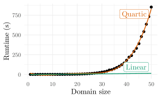
Figure 5: The runtime of FastWFOMC when counting permutations (indicated by points), together with a quartic regression model fitted on all of the data and a linear model fitted on the first half of the data points

We run FastWFOMC on an AMD Ryzen 7 5800H processor with $16\text{\,}\mathrm{GB}$ of memory, running Arch Linux 6.2.2-arch1-1 and Python 3.10.9, with $|\Delta|$ ranging from 1 to 50. The results are in Figure 5. We use ten-fold cross-validation to check the degree of the polynomial that best fits the data. The best-fitting degree is 6 with an average mean squared error (aMSE) of 16.9, although all degrees above 4 fit the data almost equally well. As Figure 5 demonstrates, a quartic (i.e., degree 4) polynomial (with an aMSE of 113.5) fits well too. However, the aMSE quickly grows to 949.5 and higher values for degrees less than 4. According to Table 1, Crane finds a cubic solution to this problem. However, we can also use the linear solution for counting bijections between different domains for this task by setting $n\coloneqq m$.

6.2 Miscellaneous Other Instances

We also note that standard (W)FOMC benchmarks such as Example 3—that are already supported by ForcLift—remain feasible for Crane as well. To demonstrate that Crane is capable of finding efficient solutions to problems beyond known domain-liftable fragments such as $\mathsf{C}^{2}$, we run Crane in greedy search mode on the following formula:

$$\begin{split}&\begin{multlined}(\forall X,W\in\Gamma\text{. }\forall Y\in\Delta\text{. }\forall Z\in\Lambda\text{. }\\ \texttt{{p}}(X,Y,Z)\land\texttt{{p}}(W,Y,Z)\Rightarrow X=W)\land{}\end{multlined}(\forall X,W\in\Gamma\text{. }\forall Y\in\Delta\text{. }\forall Z\in\Lambda\text{. }\\ \texttt{{p}}(X,Y,Z)\land\texttt{{p}}(W,Y,Z)\Rightarrow X=W)\land{}\\ &\begin{multlined}(\forall X\in\Gamma\text{. }\forall Y,W\in\Delta\text{. }\forall Z\in\Lambda\text{. }\\ \texttt{{p}}(X,Y,Z)\land\texttt{{p}}(X,W,Z)\Rightarrow Y=W).\end{multlined}(\forall X\in\Gamma\text{. }\forall Y,W\in\Delta\text{. }\forall Z\in\Lambda\text{. }\\ \texttt{{p}}(X,Y,Z)\land\texttt{{p}}(X,W,Z)\Rightarrow Y=W).\end{split}$$ (4)

For every element $z$ of $\Lambda$, Equation 4 restricts $\texttt{{p}}(X,Y,z)$ to be a $\Gamma\to\Delta$ partial injection, independent of $\texttt{{p}}(X,Y,z^{\prime})$ for any $z^{\prime}\neq z$. Crane instantly returns a solution of complexity $\Theta(l+mn)$, where $l=|\Lambda|$.

7 Discussion

This paper presents Crane—an extension of ForcLift (?) that benefits from a more general version of domain recursion and support for graphs with cycles. In Section 6, we listed a range of counting problems that became newly feasible as a result, including instances outside of currently-known domain-liftable fragments such as $\mathsf{C}^{2}$. (Although we focused on unweighted counting, ForcLift’s support for weights trivially transfers to Crane too.) The common thread across these newly liftable problems is a version of partial injectivity. Thus, we formulate the following conjecture for a class of formulas with an injectivity-like constraint on at most two parameters of a predicate p.

Conjecture 1.

Let $\mathsf{I}\mathsf{FO}^{2}$ be the class of formulas in first-order logic that contain clauses with at most two variables as well as any number of copies of

$$\begin{multlined}(\forall X_{1}\in\Delta_{1}\text{. }\dots\,\forall X_{n}\in\Delta_{n}\text{. }\forall Y\in\Delta_{i}\text{. }\texttt{{p}}(X_{1},\dots,X_{n})\land{}\\ \texttt{{p}}(X_{1},\dots,X_{i-1},Y,X_{i+1},\dots,X_{n})\Rightarrow X_{i}=Y)\land{}\end{multlined}(\forall X_{1}\in\Delta_{1}\text{. }\dots\,\forall X_{n}\in\Delta_{n}\text{. }\forall Y\in\Delta_{i}\text{. }\texttt{{p}}(X_{1},\dots,X_{n})\land{}\\ \texttt{{p}}(X_{1},\dots,X_{i-1},Y,X_{i+1},\dots,X_{n})\Rightarrow X_{i}=Y)\land{}$$

$$\begin{multlined}(\forall X_{1}\in\Delta_{1}\text{. }\dots\,\forall X_{n}\in\Delta_{n}\text{. }\forall Y\in\Delta_{j}\text{. }\texttt{{p}}(X_{1},\dots,X_{n})\land{}\\ \texttt{{p}}(X_{1},\dots,X_{j-1},Y,X_{j+1},\dots,X_{n})\Rightarrow X_{j}=Y)\end{multlined}(\forall X_{1}\in\Delta_{1}\text{. }\dots\,\forall X_{n}\in\Delta_{n}\text{. }\forall Y\in\Delta_{j}\text{. }\texttt{{p}}(X_{1},\dots,X_{n})\land{}\\ \texttt{{p}}(X_{1},\dots,X_{j-1},Y,X_{j+1},\dots,X_{n})\Rightarrow X_{j}=Y)$$

for some predicate $\texttt{{p}}/n$, domains $\Delta_{1},\dots,\Delta_{n}$, and $i,j\in\{\,1,\dots,n\,\}$. Then $\mathsf{I}\mathsf{FO}^{2}$ is liftable by Crane.

Note that the unsolved instance in Table 1 does not invalidate 1 for two reasons. First, in our experiments, the depth of the search procedure is limited, so there is a possibility that increasing the depth would make the algorithm succeed. Second, the conjecture assumes distinct domains, while the unsolved instance pertains to endofunctions.

The most important direction for future work is to automate the process in Figure 1(b). First, we need a way to find the base cases for the recursive definitions produced by Crane. Second, since the first solution found by Crane is not always optimal in terms of its complexity, an automated way to determine the asymptotic complexity of a solution would be helpful as well. Third, as we saw at the end of Example 8, the functions constructed by Crane can often benefit from elementary algebraic simplifications. This process can be automated using a computer algebra system. Furthermore, note that having the solution to a (W)FOMC problem expressed in terms of functions enables many new possibilities such as (i) the use of more sophisticated simplification techniques, (ii) asymptotic analysis of, e.g., how the model count grows as the domain size goes to infinity, and (iii) answering questions parameterised by domain sizes, e.g., ‘how big does domain $\Delta$ have to be for the probability of event $E$ to be above $95\text{\,}\mathrm{\char 37\relax}$?’

Appendix A Proofs

We begin with a few definitions that formalise the notion of a model. For any set $S$, let $2^{S}$ denote its power set and $S^{\ast}\coloneqq\bigcup_{i=0}^{\infty}S^{i}$ the (infinite) set of tuples—of any finite length—of elements of $S$. For example, ${\{\,a,b\,\}}^{\ast}=\{\,(),(a),(b),(a,a),\dots\,\}$. For any $n\in\mathbb{N}_{0}$, let $[n]\coloneqq\{\,1,\dots,n\,\}$, e.g., $[0]=\emptyset$, and $[2]=\{\,1,2\,\}$. Extending the notation for substitution introduced in Section 2, for a formula $\phi$, constant $c$, and set of variables $V$, let $\phi[c/V]$ denote $\phi$ with all occurrences of all variables in $V$ replaced with $c$. Let $\operatorname{Preds}$ be the function that maps any clause or formula to the set of predicates used in it. With each formula $\phi$, we associate a map $\pi_{\phi}\colon\operatorname{Preds}(\phi)\to{\operatorname{Doms}(\phi)}^{\ast}$ s.t., for each predicate $\texttt{{p}}/n\in\operatorname{Preds}(\phi)$, we have that $\pi_{\phi}(\texttt{{p}})\in{\operatorname{Doms}(\phi)}^{n}$. This map makes explicit the idea that each $n$-ary predicate is associated with an $n$-tuple of domains. In the case of formula $\phi$ from Example 1, $\pi_{\phi}=\{\,\texttt{{p}}\mapsto(\Gamma,\Delta)\,\}$.

Definition 5.

Let $\phi$ be a formula and $\sigma$ a domain size function. A model of $(\phi,\sigma)$ is a map $\mathfrak{M}\colon\operatorname{Preds}(\phi)\to 2^{\mathbb{N}_{0}^{\ast}}$ s.t. the following two conditions are satisfied.

1. For all predicates $\texttt{{p}}/n\in\operatorname{Preds}(\phi)$ with $\pi_{\phi}(\texttt{{p}})\coloneqq{(\Delta_{i})}_{i=1}^{n}$ for some domains $\Delta_{i}\in\operatorname{Doms}(\phi)$,

   $$\mathfrak{M}(\texttt{{p}})\subseteq\prod_{i=1}^{n}[\sigma(\Delta_{i})].$$ (5)

2. $\mathfrak{M}\models\phi$ according to the (non-exhaustive) recursive definition below. Let $\chi$ and $\psi$ be formulas, $\Delta$ a domain, $c\in\Delta$ a constant, $\texttt{{p}}/n$ a predicate associated with domains $\Delta_{1},\dots,\Delta_{n}$, and $t\in\prod_{i=1}^{n}\Delta_{i}$ a tuple of constants.

   • $\mathfrak{M}\models\texttt{{p}}(t)$ if and only if (iff) $t\in\mathfrak{M}(\texttt{{p}})$.

   • $\mathfrak{M}\models\neg\chi$ iff $\mathfrak{M}\not\models\chi$.

   • $\mathfrak{M}\models\chi\land\psi$ iff $\mathfrak{M}\models\chi$ and $\mathfrak{M}\models\psi$.

   • $\mathfrak{M}\models\chi\lor\psi$ iff $\mathfrak{M}\models\chi$ or $\mathfrak{M}\models\psi$.

   • $\mathfrak{M}\models(\forall X\in\Delta\text{. }\chi)$ iff $\mathfrak{M}\models\chi[x/\{\,X\,\}]$ for all constants $x\in\Delta$.

   • $\mathfrak{M}\models(\forall X\in\Delta\text{. }X\neq c\Rightarrow\chi)$ iff $\mathfrak{M}\models\chi[x/\{\,X\,\}]$ for all $x\in\Delta\setminus\{\,c\,\}$.

   • $\mathfrak{M}\models(\forall X,Y\in\Delta\text{. }X\neq Y\Rightarrow\chi)$ iff $\mathfrak{M}\models\chi[x/\{\,X\,\}][y/\{\,Y\,\}]$ for all $x,y\in\Delta$ s.t. $x\neq y$.

Theorem 4 (Correctness of $\operatorname{\textsc{GDR}}$).

Let $\phi$ be the formula used as input to Algorithm 1, $\Omega\in\mathcal{D}$ the domain selected on Algorithm 1, and $\phi^{\prime}$ the formula constructed by the algorithm for $\Omega$. Suppose that $\Omega\neq\emptyset$. Then $\phi\equiv\phi^{\prime}$.

Proof.

Let $x$ be the constant introduced on Algorithm 1 and $c$ a clause of $\phi$ selected on Algorithm 1 of the algorithm. We will show that $c$ is equivalent to the conjunction of clauses added to $\phi^{\prime}$ on Algorithms 1 and 1.

If $c$ has no variables with domain $\Omega$, Algorithms 1 and 1 add a copy of $c$ to $\phi^{\prime}$. If $c$ has one variable with domain $\Omega$, say, $X$, then $c\equiv\forall X\in\Omega\text{. }\psi$ for some formula $\psi$ with one free variable $X$. In this case, Algorithms 1 and 1 create two clauses: $\psi[x/\{\,X\,\}]$ and $\forall X\in\Omega\text{. }X\neq x\Rightarrow\psi$. It is easy to see that their conjunction is equivalent to $c$ provided that $\Omega\neq\emptyset$ and so $x$ is a well-defined constant.

Let $V$ be the set of variables introduced on Algorithm 1. It remains to prove that repeating the transformation

$$\forall X\in\Omega\text{. }\psi\mapsto\{\,\psi[x/\{\,X\,\}],\forall X\in\Omega\text{. }X\neq x\Rightarrow\psi\,\}$$

for all variables $X\in V$ produces the same clauses as Algorithms 1 and 1 (except for some tautologies that the latter method skips). Note that the order in which these operations are applied is immaterial. In other words, if we add inequality constraints for variables ${\{\,X_{i}\,\}}_{i=1}^{n}$, and apply substitution for variables $V\setminus{\{\,X_{i}\,\}}_{i=1}^{n}$, then—regardless of the order of operations—we get

$$\forall X_{1},\dots,X_{n}\in\Omega\text{.}\bigwedge_{i=1}^{n}X_{i}\neq x\Rightarrow\psi\left[x/\left(V\setminus{\{\,X_{i}\,\}}_{i=1}^{n}\right)\right].$$

This formula is equivalent to the clause generated on Algorithm 1 with $W=V\setminus{\{\,X_{i}\,\}}_{i=1}^{n}$. Thus, for every clause $c$ of $\phi$, the new formula $\phi^{\prime}$ gets a set of clauses whose conjunction is equivalent to $c$. Hence, the two formulas are equivalent. ∎

Theorem 5 (Correctness of $\operatorname{\textsc{CR}}$).

Let $\phi$ be the input formula of Algorithm 2, $(\Omega,x)$ a replaceable pair, and $\phi^{\prime}$ the output formula for when $(\Omega,x)$ is selected on Algorithm 2. Then $\phi\equiv\phi^{\prime}$, where the domain $\Omega^{\prime}$ introduced on Algorithm 2 is interpreted as $\Omega\setminus\{\,x\,\}$.

Proof.

Since there is a natural bijection between the clauses of $\phi$ and $\phi^{\prime}$, we shall argue about the equivalence of each pair of clauses. Let $c$ be an arbitrary clause of $\phi$ and $c^{\prime}$ its corresponding clause of $\phi^{\prime}$.

If $c$ has no variables with domain $\Omega$, then it cannot have any constraints involving $x$, so $c^{\prime}=c$. Otherwise, for notational simplicity, let us assume that $X$ is the only variable in $c$ with domain $\Omega$ (the proof for an arbitrary number of variables is virtually the same). By Definition 4, we can rewrite $c$ as $\forall X\in\Omega\text{. }X\neq x\Rightarrow\psi$, where $\psi$ is a formula with $X$ as the only free variable and with no mention of either $x$ or $\Omega$. Then $c^{\prime}\equiv\forall X\in\Omega^{\prime}\text{. }\psi$. Since $\Omega^{\prime}\coloneqq\Omega\setminus\{\,x\,\}$, we have that $c\equiv c^{\prime}$. Since $c$ was an arbitrary clause of $\phi$, this completes the proof that $\phi\equiv\phi^{\prime}$. ∎

Theorem 6 (Correctness of $\operatorname{\textsc{Ref}}$).

Let $\phi$ be the formula used as input to Algorithm 3. Let $\psi$ be any formula selected on Algorithm 3 of the algorithm s.t. $\rho\neq\texttt{{null}}$ on Algorithm 3. Let $\sigma$ be a domain size function. Then the set of models of $(\psi,\sigma\circ\rho)$ is equal to the set of models of $(\phi,\sigma)$.

Proof.

We first show that the right-hand side of Equation 5 is the same for models of both $(\phi,\sigma)$ and $(\psi,\sigma\circ\rho)$. Algorithm 3 ensures that $\psi\equiv\phi$ up to domains. In particular, this means that $\operatorname{Preds}(\psi)=\operatorname{Preds}(\phi)$. The square in

(6)

commutes by Definition 3 and the definition of $\rho$. In other words, for any predicate $\texttt{{p}}/n\in\operatorname{Preds}(\psi)=\operatorname{Preds}(\phi)$, function $\rho$ translates the domains associated with p in $\psi$ to the domains associated with p in $\phi$. Let $\pi_{\phi}(\texttt{{p}})={(\Delta_{i})}_{i=1}^{n}$ and $\pi_{\psi}(\texttt{{p}})={(\Gamma_{i})}_{i=1}^{n}$ for some domains $\Delta_{i}\in\operatorname{Doms}(\phi)$ and $\Gamma_{i}\in\operatorname{Doms}(\psi)$. Since $\rho(\Gamma_{i})=\Delta_{i}$ for all $i=1,\dots,n$ by the commutativity in Equation 6, we get that

$$\prod_{i=1}^{n}[\sigma(\Delta_{i})]=\prod_{i=1}^{n}[\sigma\circ\rho(\Gamma_{i})]$$ (7)

as required. Obviously, any subset of the left-hand side of Equation 7 (e.g., $\mathfrak{M}(\texttt{{p}})$, where $\mathfrak{M}$ is a model of $(\phi,\sigma)$) is a subset of the right-hand side and vice versa. Since $\phi$ and $\psi$ semantically only differ in what domains they refer to, every model of $\phi$ satisfies $\psi$ and vice versa, completing the proof. ∎

Appendix B Solutions Found by Crane

Here we list the exact function definitions produced by Crane for all of the problem instances in Section 6, both before and after algebraic simplification (excluding multiplications by one). The correctness of all of them has been checked by identifying suitable base cases and verifying the numerical answers across a range of domain sizes.

1. A $\Theta(m)$ solution for counting $\Gamma\to\Gamma$ functions:

   $$f(m)={\left(-1+\sum_{l=0}^{m}\binom{m}{l}[l<2]\right)}^{m}=m^{m}.$$

2. A $\Theta(m^{3}+n^{3})$ solution for counting $\Gamma\to\Delta$ surjections:

   $$f(m,n)={} \sum_{l=0}^{m}\binom{m}{l}{(-1)}^{m-l}\sum_{k=0}^{n}\binom{n}{k}{(-1)}^{n-k}$$

   $${\left(\sum_{j=0}^{k}\binom{k}{j}[j<2]\right)}^{l}$$

   $$={} \sum_{l=0}^{m}\binom{m}{l}{(-1)}^{m-l}$$

   $$\sum_{k=0}^{n}\binom{n}{k}{(-1)}^{n-k}{(k+1)}^{l}.$$

3. A $\Theta(m^{3})$ solution for counting $\Gamma\to\Gamma$ surjections:

   $$f(m)={} \sum_{l=0}^{m}\binom{m}{l}{(-1)}^{m-l}\sum_{k=0}^{m}\binom{m}{k}{(-1)}^{m-k}$$

   $${\left(\sum_{j=0}^{k}\binom{k}{j}[j<2]\right)}^{l}$$

   $$={} \sum_{l=0}^{m}\binom{m}{l}{(-1)}^{m-l}$$

   $$\sum_{k=0}^{m}\binom{m}{k}{(-1)}^{m-k}{(k+1)}^{l}.$$

4. A $\Theta(mn)$ solution for counting $\Gamma\to\Delta$ injections and partial injections (with different base cases):

   $$f(m,n)={} \sum_{l=0}^{m}\binom{m}{l}[l<2]f(m-l,n-1)$$

   $$={} f(m,n-1)+mf(m-1,n-1).$$

5. A $\Theta(m^{3})$ solution for counting $\Gamma\to\Gamma$ injections:

   $$f(m)={} \sum_{l=0}^{m}\binom{m}{l}{(-1)}^{m-l}g(m,l);$$

   $$g(m,l)={} \sum_{k=0}^{l}\binom{l}{k}[k<2]g(m-1,l-k)$$

   $$={} g(m-1,l)+lg(m-1,l-1).$$

6. A $\Theta(m)$ solution for counting $\Gamma\to\Delta$ bijections:

   $$f(m,n)=mf(m-1,n-1).$$

7. A $\Theta(l+mn)$ solution for counting $|\Lambda|$ partial injections $\Gamma\to\Delta$:

   $$f(l,m,n)={} {g(m,n)}^{l}$$

   $$g(m,n)={} \sum_{k=0}^{n}\binom{n}{k}[k<2]g(m-1,n-k)$$

   $$={} g(m-1,n)+ng(m-1,n-1).$$

References

- Barvínek et al. 2021 Barvínek, J.; van Bremen, T.; Wang, Y.; Zelezný, F.; and Kuželka, O. 2021. Automatic conjecturing of P-recursions using lifted inference. In ILP, volume 13191 of Lecture Notes in Computer Science, 17–25. Springer.
- Beame et al. 2015 Beame, P.; Van den Broeck, G.; Gribkoff, E.; and Suciu, D. 2015. Symmetric weighted first-order model counting. In PODS, 313–328. ACM.
- Chavira and Darwiche 2008 Chavira, M., and Darwiche, A. 2008. On probabilistic inference by weighted model counting. Artif. Intell. 172(6-7):772–799.
- Darwiche 2001 Darwiche, A. 2001. On the tractable counting of theory models and its application to truth maintenance and belief revision. J. Appl. Non Class. Logics 11(1-2):11–34.
- De Raedt et al. 2016 De Raedt, L.; Kersting, K.; Natarajan, S.; and Poole, D. 2016. Statistical Relational Artificial Intelligence: Logic, Probability, and Computation. Synthesis Lectures on Artificial Intelligence and Machine Learning. Morgan & Claypool Publishers.
- Dilkas 2023 Dilkas, P. 2023. Generalising weighted model counting. Ph.D. Dissertation, The University of Edinburgh.
- Gatterbauer and Suciu 2015 Gatterbauer, W., and Suciu, D. 2015. Approximate lifted inference with probabilistic databases. Proc. VLDB Endow. 8(5):629–640.
- Gogate and Domingos 2016 Gogate, V., and Domingos, P. M. 2016. Probabilistic theorem proving. Commun. ACM 59(7):107–115.
- Golia, Roy, and Meel 2020 Golia, P.; Roy, S.; and Meel, K. S. 2020. Manthan: A data-driven approach for Boolean function synthesis. In CAV (2), volume 12225 of Lecture Notes in Computer Science, 611–633. Springer.
- Gribkoff, Suciu, and Van den Broeck 2014 Gribkoff, E.; Suciu, D.; and Van den Broeck, G. 2014. Lifted probabilistic inference: A guide for the database researcher. IEEE Data Eng. Bull. 37(3):6–17.
- Jaeger and Van den Broeck 2012 Jaeger, M., and Van den Broeck, G. 2012. Liftability of probabilistic inference: Upper and lower bounds. In StarAI@UAI.
- Kazemi and Poole 2016 Kazemi, S. M., and Poole, D. 2016. Knowledge compilation for lifted probabilistic inference: Compiling to a low-level language. In KR, 561–564. AAAI Press.
- Kazemi et al. 2016 Kazemi, S. M.; Kimmig, A.; Van den Broeck, G.; and Poole, D. 2016. New liftable classes for first-order probabilistic inference. In NIPS, 3117–3125.
- Kersting 2012 Kersting, K. 2012. Lifted probabilistic inference. In ECAI, volume 242 of Frontiers in Artificial Intelligence and Applications, 33–38. IOS Press.
- Kimmig, Mihalkova, and Getoor 2015 Kimmig, A.; Mihalkova, L.; and Getoor, L. 2015. Lifted graphical models: A survey. Mach. Learn. 99(1):1–45.
- Kuncak et al. 2010 Kuncak, V.; Mayer, M.; Piskac, R.; and Suter, P. 2010. Complete functional synthesis. In PLDI, 316–329. ACM.
- Kuusisto and Lutz 2018 Kuusisto, A., and Lutz, C. 2018. Weighted model counting beyond two-variable logic. In LICS, 619–628. ACM.
- Kuželka 2021 Kuželka, O. 2021. Weighted first-order model counting in the two-variable fragment with counting quantifiers. J. Artif. Intell. Res. 70:1281–1307.
- Malhotra and Serafini 2022 Malhotra, S., and Serafini, L. 2022. Weighted model counting in FO2 with cardinality constraints and counting quantifiers: A closed form formula. In AAAI, 5817–5824. AAAI Press.
- Niu et al. 2011 Niu, F.; Ré, C.; Doan, A.; and Shavlik, J. W. 2011. Tuffy: Scaling up statistical inference in Markov logic networks using an RDBMS. Proc. VLDB Endow. 4(6):373–384.
- Richardson and Domingos 2006 Richardson, M., and Domingos, P. M. 2006. Markov logic networks. Mach. Learn. 62(1-2):107–136.
- Sanathanan and Koerner 1963 Sanathanan, C., and Koerner, J. 1963. Transfer function synthesis as a ratio of two complex polynomials. IEEE transactions on automatic control 8(1):56–58.
- van Bremen and Kuželka 2020 van Bremen, T., and Kuželka, O. 2020. Approximate weighted first-order model counting: Exploiting fast approximate model counters and symmetry. In IJCAI, 4252–4258. ijcai.org.
- van Bremen and Kuželka 2021a van Bremen, T., and Kuželka, O. 2021a. Faster lifting for two-variable logic using cell graphs. In UAI, volume 161 of Proceedings of Machine Learning Research, 1393–1402. AUAI Press.
- van Bremen and Kuželka 2021b van Bremen, T., and Kuželka, O. 2021b. Lifted inference with tree axioms. In KR, 599–608.
- Van den Broeck et al. 2011 Van den Broeck, G.; Taghipour, N.; Meert, W.; Davis, J.; and De Raedt, L. 2011. Lifted probabilistic inference by first-order knowledge compilation. In IJCAI, 2178–2185. IJCAI/AAAI.
- Van den Broeck, Choi, and Darwiche 2012 Van den Broeck, G.; Choi, A.; and Darwiche, A. 2012. Lifted relax, compensate and then recover: From approximate to exact lifted probabilistic inference. In UAI, 131–141. AUAI Press.
- Van den Broeck, Meert, and Darwiche 2014 Van den Broeck, G.; Meert, W.; and Darwiche, A. 2014. Skolemization for weighted first-order model counting. In KR. AAAI Press.
- Van den Broeck 2011 Van den Broeck, G. 2011. On the completeness of first-order knowledge compilation for lifted probabilistic inference. In NIPS, 1386–1394.
- Venugopal, Sarkhel, and Gogate 2015 Venugopal, D.; Sarkhel, S.; and Gogate, V. 2015. Just count the satisfied groundings: Scalable local-search and sampling based inference in MLNs. In AAAI, 3606–3612. AAAI Press.