The Role of Fine-tuning: Transfer Learning for High-dimensional M-estimators with Decomposable Regularizers

Zeyu Li 111Department of Statistics and Data Science, School of Management at Fudan University, China; e-mail:zeyuli21@m.fudan.edu.cn; xszhang@fudan.edu.cn 444The authors contributed equally to this work., Dong Liu 222School of Statistics and Management, Shanghai University of Finance and Economics, China; e-mail:liudong@163.sufe.edu.cn 44footnotemark: 4, Yong He, 333Institute for Financial Studies, Shandong University, China; e-mail:heyong@sdu.edu.cn Xinsheng Zhang 11footnotemark: 1
Abstract

Transfer learning algorithms have been developed in various applicational contexts while only a few of them offer statistical guarantees in high-dimensions. Among these work, the differences between the target and sources, a.k.a. the contrasts, are typically modeled as, or at least close to, vectors with certain low-dimensional structure (e.g., sparsity), resulting in a separate debiasing step after a preceding pooling estimation procedure. Under such intuitive yet powerful framework, additional homogeneity conditions on Hessian matrices of the population loss functions are often imposed to preserve the delicate low-dimensional structure of the contrasts during pooling, which is either unrealistic in practice or easily destroyed by basic data transformation such as standardization. In this article, under the general M-estimators framework with decomposable regularizers, we highlight the role of fine-tuning underneath the conspicuous gain of the debiasing step in transfer learning. Namely, we find it is possible to enhance estimation accuracy by fine-tuning a primal estimator sufficiently close to the true target one. Our theory suggests slightly enlarging the pooling regularization strength when either the contrast’s low-dimensional structure or the homogeneity of Hessian matrices is violated. Traditional linear regression and generalized low-rank trace regression in high-dimensions are discussed as two specific examples under our framework. When the informative source datasets are unknown, a novel truncated-penalized algorithm is proposed to directly output the primal estimator by simultaneously selecting the useful sources and its oracle property is proved. Extensive numerical experiments are conducted to validate the theoretical assertions. A case study on the air quality regulation in China by transfer learning is also provided for illustration.


Keywords: Decomposable regularizer; M-estimators; Trace regression; Transfer learning; Truncated norm penalty.

1 Introduction

The idea of transfer learning, originated from the computer science community (Torrey and Shavlik,, 2010; Zhuang et al.,, 2020; Niu et al.,, 2020), has been applied to various high-dimensional statistical problems in the past few years. As its name indicates, useful information from related tasks (sources) could be transferred to the original task (target), so as to improve the efficiency of statistical inference for the latter. Bastani, (2021) first proposes a two-step transfer learning algorithm when the source data size is sufficiently large and the difference between the target and source tasks can be modeled as a sparse function. Li et al., 2022a discuss the transfer learning problem under the high-dimensional linear model setting and establish the minimax optimal rate for the estimators of the target parameters. Tian and Feng, (2022) further study the estimation and inference for generalized linear model under the transfer learning framework. Both Li et al., 2022a and Tian and Feng, (2022) focus on a two-step transfer learning procedure: in the first step a primal estimator of the target parameter is acquired by pooling the useful datasets, and in the second step the primal estimator is then debiased with only the target data. Intuitively, when the sources are sufficiently close to the target, transfer learning would outperform the direct inference procedure by just using the target dataset. For the benefit of knowledge transfer under various statistical models, one may also refer to Qiao et al., (2023) for quantile regression, Li et al., 2022b ; He et al., (2022) for Gaussian/semi-parametric graphical models, and Cai and Wei, (2021); Reeve et al., (2021) for non-parametric classification.

For high-dimensional statistical inference problems, additional low-dimensional structures are often imposed on the model parameters, so that consistent estimators can be obtained. One typical example is the sparse signal assumption, i.e., assuming the sparsity of model parameters of interest (Tibshirani,, 1996; Fan and Li,, 2001; Candes and Tao,, 2007). When the parameters of interest arise in the matrix form, an alternative model assumption would be low-rankness, which has been widely explored and applied in the communities of statistics, computer science and econometrics (Zhou and Li,, 2014; Fan et al., 2019a, ; He et al.,, 2023).

In this article, we consider the transfer learning problem under the high-dimensional M-estimators framework with decomposable regularizers following Negahban et al., (2012). We denote the target dataset as ${\mathbb{D}}_{0}$ and $K$ potential source datasets as ${\mathbb{D}}_{k}$, $k=1,\cdots,K$, whose population parameters are denoted as $\bm{\theta}^{*}_{k}\in{\mathbb{R}}^{p}$, $k=0,\cdots,K$. We assume that $\bm{\theta}^{*}_{k}$ is the minimizer of the expected loss function, i.e.,

$$\bm{\theta}^{*}_{k}=\mathop{\text{\rm arg\,min}}_{\bm{\theta}\in{\mathbb{R}}^{p}}{\mathbb{E}}\ \mathcal{L}_{k}(\bm{Z}_{k};\bm{\theta}),\quad\bm{Z}_{k}\text{ is sampled from }{\mathbb{D}}_{k},$$

where $\mathcal{L}_{k}(\cdot;\bm{\theta})$ is the loss function of the $k$-th study. We assume that $\bm{\theta}^{*}_{0}$ lies in a low-dimensional subspace ${\mathcal{M}}\subset{\mathbb{R}}^{p}$. For instance, it might be the subspace of vectors with a particular support or the subspace of low-rank matrices. Denote the inner product induced norm as $\|\cdot\|^{2}=\langle\cdot,\cdot\rangle$. Given subspace $\overline{{\mathcal{M}}}$ such that ${\mathcal{M}}\subset\overline{{\mathcal{M}}}$, let $\overline{{\mathcal{M}}}^{\perp}=\{\bm{v}\in{\mathbb{R}}^{p}\,|\,\langle\bm{u},\bm{v}\rangle=0\text{ for all }\bm{u}\in\overline{{\mathcal{M}}}\}$ be the orthogonal complement of the space $\overline{{\mathcal{M}}}$, we say a norm-based regularizer (or penalty) ${\mathcal{R}}$ is decomposable with respect to $({\mathcal{M}},\overline{{\mathcal{M}}}^{\perp})$ if

$${\mathcal{R}}(\bm{\theta}+\bm{\gamma})={\mathcal{R}}(\bm{\theta})+{\mathcal{R}}(\bm{\gamma}),\quad\text{for all }\bm{\theta}\in{\mathcal{M}}\text{ and }\bm{\gamma}\in\overline{{\mathcal{M}}}^{\perp}.$$

For the sake of better illustration, we present here several examples of the decomposable regularizers given in Negahban et al., (2012), while some other useful results therein are stated in the Appendix for convenience.

Example 1.1 (Sparse vector and $\ell_{1}$ norm).

Suppose that $\bm{\theta}^{*}_{0}$ is supported on some subset $S\subset\{0,1,\dots,p\}$ with cardinality $s$, we set $\mathcal{M}=\overline{\mathcal{M}}=\{\bm{\theta}\in{\mathbb{R}}^{p}\mid\bm{\theta}_{j}=0\text{ for all }j\notin S\}$. We can take $\mathcal{R}(\cdot)=\|\cdot\|_{1}$, it is easy to verify that $\|\bm{\theta}+\bm{\gamma}\|_{1}=\|\bm{\theta}\|_{1}+\|\bm{\gamma}\|_{1}$ for all $\bm{\theta}\in{\mathcal{M}}$ and $\bm{\gamma}\in\overline{{\mathcal{M}}}^{\perp}$ by the construction of the subspaces.

Example 1.2 (Group structured norms).

In many cases, sparsity arises in a more structured form, namely groups of coefficients are likely to be zero simultaneously. Suppose the index set could be partitioned into $n_{\mathcal{G}}$ disjoint groups $\{g_{1},g_{2},\dots,g_{n_{\mathcal{G}}}\}$. For $\alpha\in[1,\infty]$, we define the $(1,\alpha)$-group norm as $\|\bm{\theta}\|_{\mathcal{G},\alpha}=\sum_{t=1}^{n_{\mathcal{G}}}\|\bm{\theta}_{g_{t}}\|_{\alpha}$, where $\bm{\theta}_{g_{t}}$ means the projection of $\bm{\theta}$ onto the support $g_{t}$. Note that for $\alpha=1$, we obtain the standard $\ell_{1}$ norm. Given any subset $S_{\mathcal{G}}\subset\{1,\dots,n_{\mathcal{G}}\}$ of group indices, with cardinality $s_{\mathcal{G}}$, we can take $\mathcal{M}=\overline{\mathcal{M}}=\{\bm{\theta}\in{\mathbb{R}}^{p}\mid\bm{\theta}_{g_{t}}=\mathbf{0}\text{ for all }t\notin S_{\mathcal{G}}\}$, and the $(1,\alpha)$-group norm is decomposable with respect to $({\mathcal{M}},\overline{{\mathcal{M}}}^{\perp})$.

Example 1.3 (Low rank matrix and nuclear norm).

Let $\bm{\theta}^{*}_{0}$ be a low rank matrix, and let $\bm{\theta}^{*}_{0}=\bm{U}\bm{D}\bm{V}^{\top}$ be its singular value decomposition (SVD), where $\bm{D}$ is a diagonal matrix that consists of non-increasing singular values. Denote the first $r$ columns of $\bm{U}$ and $\bm{V}$ by $\bm{U}^{r}$ and $\bm{V}^{r}$, we take

$$\bm{\theta}^{*}_{0}\in\mathcal{M}:=\left\{\bm{\theta}\in\mathbb{R}^{d_{1}\times d_{2}}\mid\operatorname{row}(\bm{\theta})\subseteq\operatorname{col}\left(\mathbf{V}^{r}\right),\operatorname{col}(\bm{\theta})\subseteq\operatorname{col}\left(\mathbf{U}^{r}\right)\right\},$$ (1)
$$\overline{\mathcal{M}}^{\perp}:=\left\{\bm{\theta}\in\mathbb{R}^{d_{1}\times d_{2}}\mid\operatorname{row}(\bm{\theta})\perp\operatorname{col}\left(\mathbf{V}^{r}\right),\operatorname{col}(\bm{\theta})\perp\operatorname{col}\left(\mathbf{U}^{r}\right)\right\},$$ (2)

where $\operatorname{col}(\cdot)$ and $\operatorname{row}(\cdot)$ denote spaces spanned by columns and rows respectively. It is known that the matrix nuclear norm $\|\cdot\|_{N}$ satisfies the decomposability condition. Note that in this case ${\mathcal{M}}$ is not equal to $\overline{{\mathcal{M}}}$.

The superiority of the M-estimators framework is two-fold: first, the statistical reasoning concerning transfer learning can be conveyed more clearly in a general sense; second, the developed theory and methods can be directly applied to specific statistical models. For instance, let ${\mathbb{D}}_{k}$ consist of $n_{k}$ i.i.d. observations of $\bm{Z}_{k,i}=(\bm{X}_{k,i},y_{k,i})$, set

$$y_{k,i}=\langle\bm{\theta}^{*}_{k},\bm{X}_{k,i}\rangle+\varepsilon_{k,i},$$ (3)

where $\varepsilon_{k,i}$ are standard Gaussian errors. Hence $\bm{\theta}^{*}_{k}$ is the minimizer of the expected loss function ${\mathbb{E}}\|y_{k}-\langle\bm{\theta},\bm{X}_{k}\rangle\|^{2}$. If $\bm{\theta}^{*}_{0}$ is sparse, then we could take $\mathcal{R}=\|\cdot\|_{1}$ and the problem degenerates to the transfer learning problem for linear regression discussed in Li et al., 2022a . On the other hand, if $\bm{\theta}^{*}_{0}$ is a low rank matrix, then we take $\mathcal{R}=\|\cdot\|_{N}$ and consider a transfer learning problem for trace regression. Trace regression is introduced in Zhou and Li, (2014) and is particularly useful in modeling matrix completion, multi-task learning and compressed sensing problems (Hamdi and Bayati,, 2022). For more examples, one may consider the generalized linear model

$${\mathbb{P}}(y_{k,i}|\bm{X}_{k,i})\propto\exp\left\{y_{k,i}\langle\bm{\theta}^{*}_{k},\bm{X}_{k,i}\rangle-b(\langle\bm{\theta}^{*}_{k},\bm{X}_{k,i}\rangle)\right\},$$

where $\bm{\theta}^{*}_{k}=\mathop{\text{\rm arg\,min}}_{\bm{\theta}\in{\mathbb{R}}^{p}}{\mathbb{E}}\left\{-y_{k}\langle\bm{\theta},\bm{X}_{k}\rangle+b(\langle\bm{\theta},\bm{X}_{k}\rangle)\right\}$. The problem then degenerates to the one discussed in Tian and Feng, (2022) if $\bm{\theta}^{*}_{0}$ is sparse, or to the transfer learning problem for generalized trace regression if $\bm{\theta}^{*}_{0}$ is of low rank. Generalized trace regression and related applications, including generalized reduced-rank regression and one-bit matrix completion, are thoroughly discussed in Fan et al., 2019a .

To measure the informative level of the $k$-th source dataset, we resort to the magnitude of the contrast vector $\bm{\delta}^{*}_{k}=\bm{\theta}^{*}_{0}-\bm{\theta}^{*}_{k}$ with respect to some norm $\mathcal{B}_{k}$. For the informative sources $\mathcal{A}\subset\{1,\cdots K\}$, we assume

$$\mathcal{B}_{k}(\bm{\delta}^{*}_{k})\leq h,\quad k\in\mathcal{A},$$ (4)

where smaller $h$ indicates higher similarity. For example, $\mathcal{B}_{k}$ can be the vector $\ell_{1}$ or $\ell_{2}$ norm in the case of sparse linear regression. For generalized trace regression, it can be the nuclear norm, the Frobenius norm or the vectorized $\ell_{1}$ norm. As for $k\in\mathcal{A}^{c}$, $\bm{\theta}^{*}_{k}$ is allowed to be quite different from $\bm{\theta}^{*}_{0}$.

1.1 Closely-Related Work and Our Contributions

First consider the case that the informative sources are known in advance, or equivalently all sources included are useful, i.e., $\mathcal{A}=\{1,\cdots,K\}$, we name this scenario as oracle transfer learning. One natural way under this setting is to first pool all the datasets and estimate the population pooling parameter

$$\bm{\theta}^{*}_{\mathcal{P}}=\mathop{\text{\rm arg\,min}}\sum_{k\in\mathcal{P}}\frac{n_{k}}{n_{\mathcal{P}}}{\mathbb{E}}\left[\mathcal{L}_{k}(\bm{Z}_{k};\bm{\theta})\right],$$

for $\mathcal{P}=\{0\}\cup\mathcal{A}$ and $n_{\mathcal{P}}=\sum_{k\in{\mathcal{P}}}n_{k}$ (Li et al., 2022a, ; Tian and Feng,, 2022). The existing literature tends to credit the advantage of transfer learning to the simplified problem of estimating the difference $\bm{\theta}^{*}_{\mathcal{P}}-\bm{\theta}^{*}_{0}$. For better performance of transfer learning, such difference is typically required to be even more sparse than $\bm{\theta}^{*}_{0}$, by assuming each contrast vector $\bm{\delta}^{*}_{k}$ to be sufficiently sparse. For instance, Li et al., 2022a assumes that $\|\bm{\delta}^{*}_{k}\|_{q}\leq h$ for $q\in[0,1]$, while Tian and Feng, (2022) assumes $\|\bm{\delta}^{*}_{k}\|_{1}\leq h$. Recall that $\ell_{0}$ norm is often used to measure strong sparsity while $\ell_{1}$ norm is for weak sparsity.

Refer to caption
Figure 1: Frequencies of the best performing estimators in the transfer learning framework for linear regression based on $100$ numerical experiments, with $K=4$, $n_{0}=n_{k}=500$, $p=1000$, and heterogeneous covariance matrices of the covariates. We set $95\%$ of the entries of $\bm{\theta}^{*}_{0}$ as 0, while elements of $\bm{\delta}^{*}_{k}$ are taken independently from $N(0,h^{2}/p)$, so that $\|\bm{\delta}^{*}_{k}\|_{1}\asymp hp^{1/2}$ and $\|\bm{\delta}^{*}_{k}\|_{2}\asymp h$. $\widehat{\bm{\theta}}_{v}$ stands for the vanilla target estimator, $\widehat{\bm{\theta}}_{\mathcal{P}}$ is the pooling estimator after slightly enlarging the regularization parameter selected by cross validation, while $\widehat{\bm{\theta}}^{\star}_{\mathcal{P}}$ is its fine-tuned version.

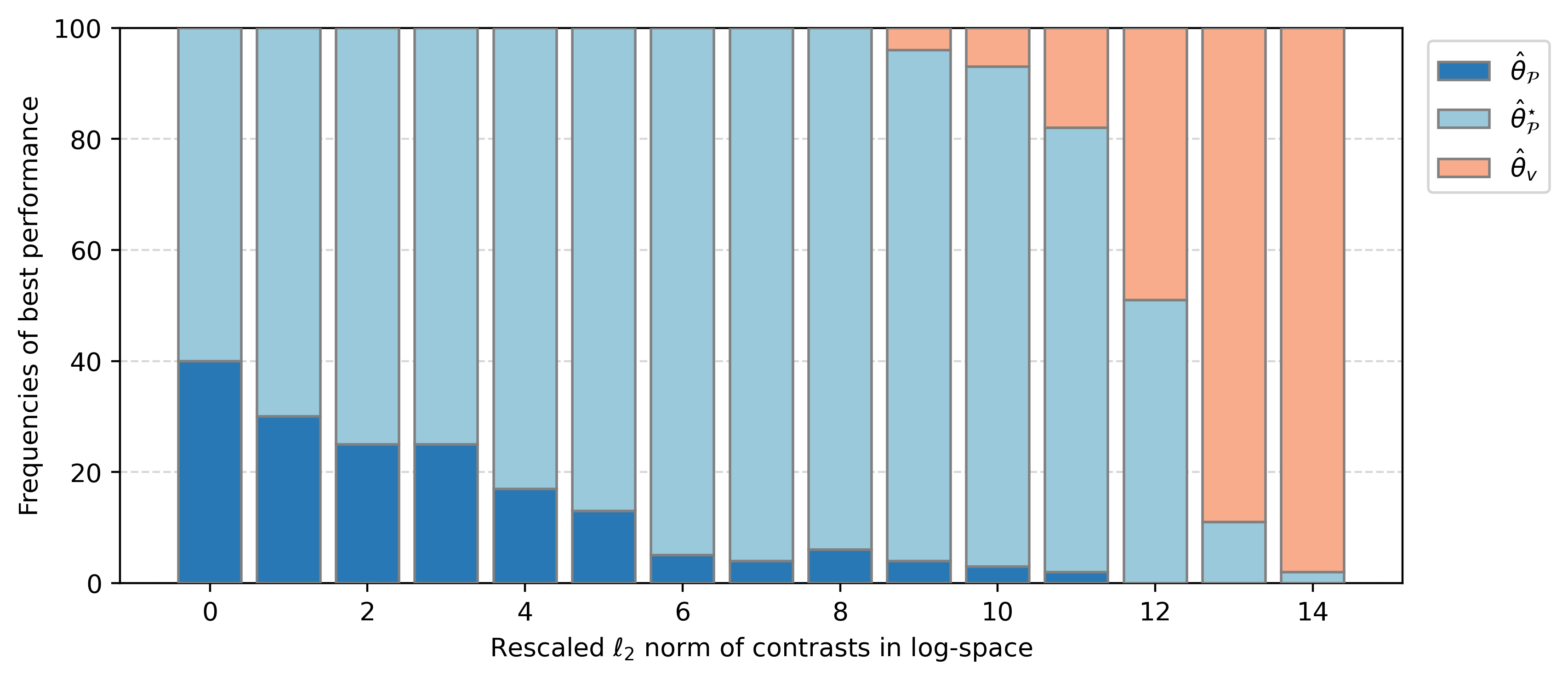
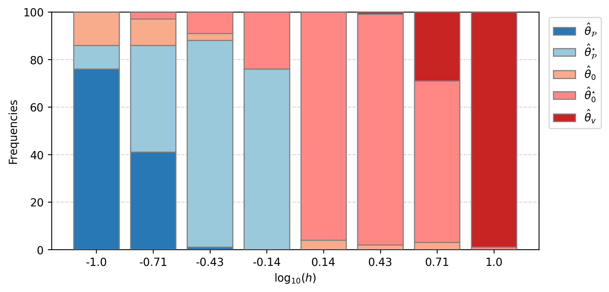
However, the low-dimensional structure of $\bm{\delta}^{*}_{k}$ is a delicate property which is either unrealistic in practice or easily destroyed by basic data transformation such as standardization. To preserve it during the pooling step, additional homogeneity conditions on Hessian matrices of the population loss functions are often imposed. That is to say, although such ideology is powerful enough to explain a large portion of the conspicuous gain obtained by transfer learning, it provides less guidance if either the individual contrast $\bm{\delta}^{*}_{k}$ has no low-dimensional structure in nature or the Hessian matrices are heterogeneous. For better illustration, we report in Figure 1 the frequencies of the best performing estimators under the transfer learning framework for linear regression, based on $100$ numerical experiments, where the covariance matrices of the covariates are heterogeneous and the contrast vectors are small only in $\ell_{2}$ norm but relatively large in $\ell_{1}$ norm. While the difference $\bm{\theta}^{*}_{\mathcal{P}}-\bm{\theta}^{*}_{0}$ is almost unlikely to be sparse, both the pooling estimator $\widehat{\bm{\theta}}_{\mathcal{P}}$, with suitable regularization strength, and its fine-tuned version $\widehat{\bm{\theta}}^{\star}_{\mathcal{P}}$ outperform the vanilla target estimator $\widehat{\bm{\theta}}_{v}$ given sufficiently small $\ell_{2}$ norm of the contrasts. In essence, the dominance of $\widehat{\bm{\theta}}^{\star}_{\mathcal{P}}$ in the moderate $\ell_{2}$-contrast regime cannot be explained by the existing theoretical frameworks discussed in Li et al., 2022a ; Tian and Feng, (2022).

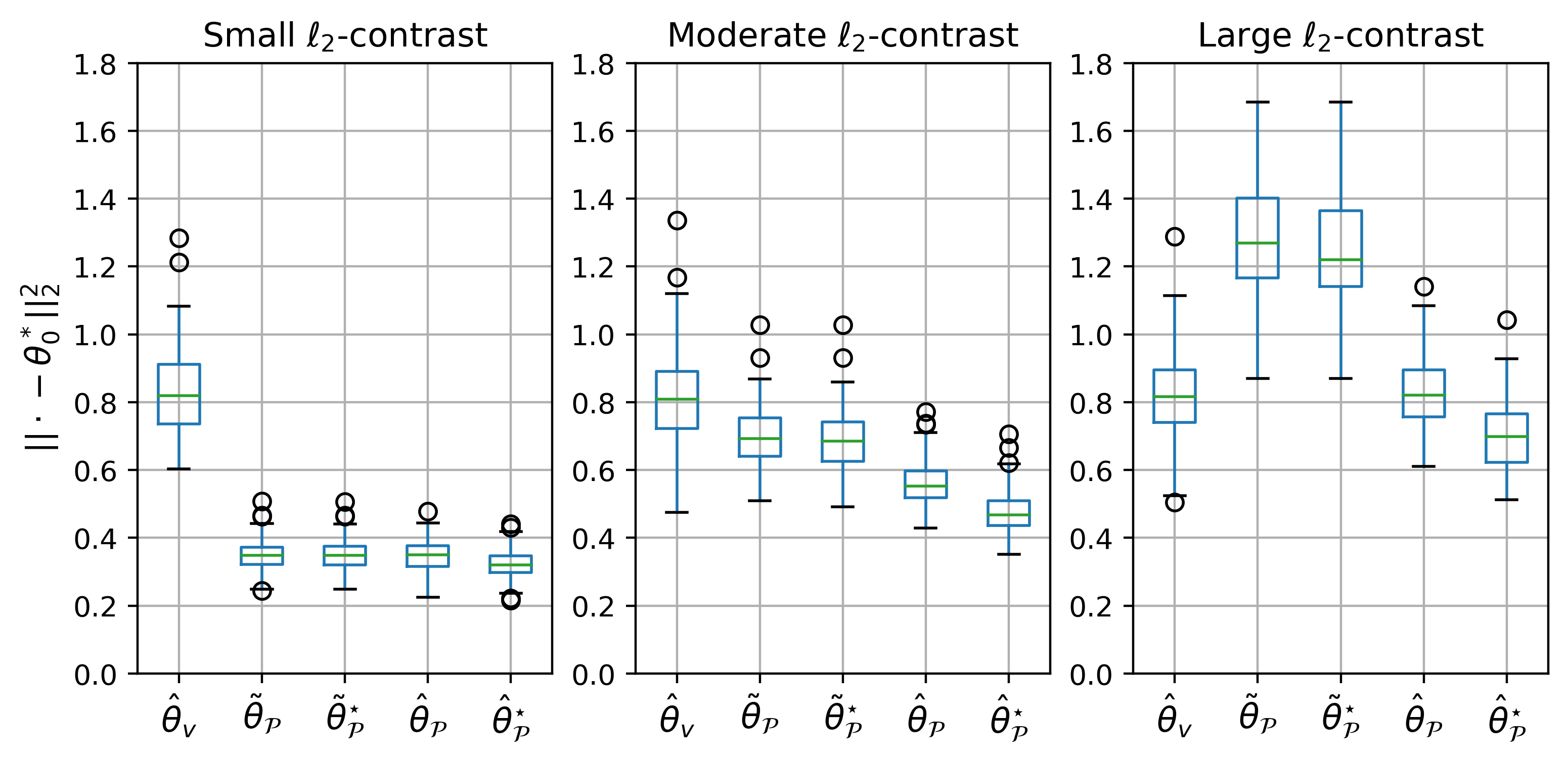
Our first main contribution is to highlight the role of fine-tuning under the general M-estimators framework with decomposable regularizers. Namely, it is still possible to enhance estimation accuracy by fine-tuning a primal estimator sufficiently close to the true target one. To harness this alternative effect, our theoretical analysis shows that it’s better slightly enlarging the classical pooling regularization parameter targeting at $\bm{\theta}^{*}_{\mathcal{P}}$ to acquire a more informative primal estimator, if either the low-dimensional structure of contrasts or the homogeneity of Hessian matrices is violated. In Figure 2, we present the box-plots of the estimation error of various estimators under the same settings as for Figure 1, where $\widetilde{\bm{\theta}}_{\mathcal{P}}$ is the pooling estimator with regularizing parameter selected by cross validation. On the other hand, $\widehat{\bm{\theta}}_{\mathcal{P}}$ is the estimator corresponding to slightly enlarging the regularization strength. We can see that $\widehat{\bm{\theta}}_{\mathcal{P}}$ contains more primal information than $\widetilde{\bm{\theta}}_{\mathcal{P}}$, as the former’s fine-tuned version $\widehat{\bm{\theta}}^{\star}_{\mathcal{P}}$ tends to have the smallest error, particularly in the moderate $\ell_{2}$-contrast regime. Then, transfer learning procedures of specific statistical models are discussed within the M-estimators framework, including that of the generalized trace regression which, to the best of our knowledge, has not been discussed in the existing literature and is of independent interest.

Refer to caption
Figure 2: Box-plots of the estimation error, as measured in $\|\cdot-\bm{\theta}^{*}_{0}\|^{2}_{2}$, of various estimators under the same settings as for Figure 1. $\widehat{\bm{\theta}}_{v}$ stands for the vanilla target estimator, $\widetilde{\bm{\theta}}_{\mathcal{P}}$ and $\widehat{\bm{\theta}}_{\mathcal{P}}$ are the pooling estimators before and after slightly enlarging the regularizing parameter obtained by cross validation, respectively, while $\widetilde{\bm{\theta}}^{\star}_{\mathcal{P}}$ and $\widehat{\bm{\theta}}^{\star}_{\mathcal{P}}$ are their fine-tuned versions.

In practice, the useful source datasets are usually unknown, and transferring information from irrelevant sources can be very harmful, known as “negative transfer” in the literature (Torrey and Shavlik,, 2010). To avoid negative transfer, Li et al., 2022a take advantage of model selection aggregation, while Tian and Feng, (2022) propose a data-driven method to detect the transferable sources.

The second main contribution of this work is to introduce the truncated norm penalty into the transfer learning problem with the intuition of dataset clustering. The truncated norm penalty is originally introduced by Shen et al., (2012) to replace $\ell_{1}$ penalty in high-dimensional linear regression, and is further utilized by Pan et al., (2013); Wu et al., (2016); Liu et al., (2023) to alleviate the bias of estimating group centroids in the clustering analysis. The main idea of our method is to automatically incorporate those sources with high informative level into the estimation procedure of the target parameters. In contrast to the existing methods focusing on identifying useful dataset as a separate step, our algorithm directly outputs the primal estimator by simultaneously selecting the useful sources. Thus it is computationally more efficient, particularly when the number of the candidate sources is large. The truncated-penalized estimator is proved to be as good as the oracle pooling estimator under mild conditions, which is named as the oracle property in this paper.

As a concurrent work, Li et al., (2023) propose to jointly estimate the target parameters and the contrast vectors in one single step for the generalized linear model, assuming sufficiently sparse contrasts. Their theoretical arguments quantify the gain from such joint estimation procedure, and fit to cases with heterogeneous Hessian matrices. As shown by simulation, our truncated-penalized algorithm also benefits from the one-step joint estimation under sparse contrasts. Compared to their method, our algorithm possesses the additional advantage of simultaneous dataset selection thanks to the truncated-penalization.

1.2 Paper Organization and Notations

The remainder of this work is organized as follows. In section 2 we propose the two-step transfer learning methods given informative datasets either known or unknown. Related theoretical arguments are then presented in section 3. In the end, numerical simulation results and algorithm details are given in section 4. A real case study on the air quality regulation in China is presented in section 5.

To end this section, we introduce some notations used throughout the paper. The inner product induced norm $\|\cdot\|$ is sometimes written as $\|\cdot\|_{2}$ for vectors or $\|\cdot\|_{F}$ for matrices. For real vector $\bm{a}$, let $\|\bm{a}\|_{1}$ be its $\ell_{1}$-norm, while for real matrix $\bm{A}$, let $\|\bm{A}\|_{\text{op}}$ and $\|\bm{A}\|_{N}$ be its operator norm (from $\ell_{2}$ to $\ell_{2}$) and nuclear norm respectively. We use the standard $O_{p}$ notation for stochastic boundedness. For a sub-Gaussian random variable $X$, we define the sub-Gaussian norm by $\|X\|_{\psi_{2}}=\inf\left\{t>0:\mathbb{E}\exp\left(X^{2}/t^{2}\right)\leq 2\right\}$, while for a random vector $\bm{X}$, its sub-Gaussian norm is defined as $\|\bm{X}\|_{\psi_{2}}=\sup_{\|\bm{x}\|_{2}=1}\|\langle\bm{X},\bm{x}\rangle\|_{\psi_{2}}$. In the end, we write $x\lesssim y$ if $x\leq Cy$ for some $C>0$, $x\gtrsim y$ if $x\geq cy$ for some $c>0$, and $x\asymp y$ if both $x\lesssim y$ and $x\gtrsim y$ hold. Note that the constants $C$ and $c$ may not be identical in different lines.

2 Methodology

In section 2.1, we introduce the two-step, i.e., the pooling and the fine-tuning steps, transfer learning method when all datasets ${\mathbb{D}}_{k}$ are informative. We remark on the subtle difference between our theoretical framework and the existing ones in section 2.2. When the informative datasets are unknown, a truncated-penalized algorithm is proposed in section 2.3 to select useful sources.

2.1 Oracle Transfer Learning Algorithm

First consider the oracle transfer learning scenario where all source datasets are informative, namely $\mathcal{A}=\{1,\cdots,K\}$, recall that $\bm{\theta}^{*}_{0}\in{\mathcal{M}}\subset\overline{{\mathcal{M}}}$ and the norm-based regularizer ${\mathcal{R}}$ is decomposable with respect to $({\mathcal{M}},\overline{{\mathcal{M}}}^{\perp})$. Following Li et al., 2022a ; Tian and Feng, (2022), we first include ${\mathbb{D}}_{0}$ by setting $\mathcal{P}=\{0\}\cup\mathcal{A}$, and acquire the initial estimator $\widehat{\bm{\theta}}_{{\mathcal{P}}}$ by weighted-pooling:

$$\widehat{\bm{\theta}}_{\mathcal{P}}=\mathop{\text{\rm arg\,min}}_{\bm{\theta}\in{\mathbb{R}}^{p}}\frac{1}{n_{\mathcal{P}}}\sum_{k\in\mathcal{P}}\sum_{i\leq n_{k}}\alpha_{k}\mathcal{L}_{k}(\bm{Z}_{k,i};\bm{\theta})+\lambda_{\mathcal{P}}{\mathcal{R}}(\bm{\theta}),$$ (5)

where $n_{\mathcal{P}}=\sum_{k\in\mathcal{P}}n_{k}$ and $(\alpha_{1},\cdots,\alpha_{K})$ are given weights to make $\alpha_{k}\mathcal{L}_{k}$ comparable. For instance, for the linear regression model in (3), if $\text{Var}(\varepsilon_{k,i})=\sigma^{2}_{k}$, it is natural to set $\alpha_{k}=1/\sigma^{2}_{k}$. We typically set $\alpha_{k}=1$ in this work without loss of generality.

If the primal estimator $\widehat{\bm{\theta}}_{\mathcal{P}}$ is sufficiently close to $\bm{\theta}^{*}_{0}$, namely ${\mathcal{R}}(\widehat{\bm{\theta}}_{\mathcal{P}}-\bm{\theta}^{*}_{0})\leq l_{{\mathcal{P}}}$ for some $l_{{\mathcal{P}}}>0$ with high probability, in the second step we fine-tune the parameter by solving the constrained optimization

$$\widehat{\bm{\theta}}^{\star}_{\mathcal{P}}=\mathop{\text{\rm arg\,min}}_{\theta\in{\mathbb{R}}^{p}}\frac{1}{n_{0}}\sum_{i\leq n_{0}}\mathcal{L}_{0}(\bm{Z}_{0,i};\bm{\theta}),\quad\text{subject to }{\mathcal{R}}(\widehat{\bm{\theta}}_{\mathcal{P}}-\bm{\theta})\leq l_{{\mathcal{P}}}.$$ (6)

For $\widehat{\bm{\delta}}=\widehat{\bm{\theta}}^{\star}_{\mathcal{P}}-\widehat{\bm{\theta}}_{\mathcal{P}}$, the optimization problem above has the familiar and more practical Lagrangian form with a slight abuse of notations (note that these two problems are not mathematically equivalent but we use the same $\widehat{\bm{\theta}}^{\star}_{\mathcal{P}}$ and $\widehat{\bm{\delta}}$ to denote the solutions):

$$\widehat{\bm{\delta}}=\mathop{\text{\rm arg\,min}}_{\bm{\delta}\in{\mathbb{R}}^{p}}\frac{1}{n_{0}}\sum_{i\leq n_{0}}\mathcal{L}_{0}(\bm{Z}_{0,i};\widehat{\bm{\theta}}_{\mathcal{P}}+\bm{\delta})+\lambda_{d}{\mathcal{R}}(\bm{\delta}).$$ (7)

The role of fine-tuning might be better understood via the constrained form (6). That is, from the target and source datasets we acquire knowledge on where $\bm{\theta}^{*}_{0}$ might locate with high probability, then the fine-tuned estimator outperforms direct estimation using only the target dataset if such primal information is reliable enough. In this work, we use the weighted-pooling $\widehat{\bm{\theta}}_{\mathcal{P}}$ as the primal estimator, which is not the only choice. In fact, in some real applications where the size of source data sets are too large to pool, while some well-behaved estimators are available in advance, it is also acceptable to use them as primal estimators directly.

Also, note that the second fine-tuning step is not always necessary. Consider the extreme case where $h=0$, there is no need of fine-tuning since it only adds additional variance from the target dataset. If $l_{\mathcal{P}}$ (or $\lambda_{d}$) is chosen to be sufficiently small (or large) in this case, then we have $\widehat{\bm{\delta}}=0$ and $\widehat{\bm{\theta}}^{\star}_{\mathcal{P}}=\widehat{\bm{\theta}}_{\mathcal{P}}$ as if the second step does not exist. Empirically, we suggest choosing the tuning parameter of the fine-tuning step via cross validation.

Algorithm 1 Oracle transfer learning for M-estimators.
0:    the target dataset ${\mathbb{D}}_{0}$ and informative source datasets ${\mathbb{D}}_{k}$, $k=1,\cdots,K$;tuning parameters: weights $(\alpha_{k})_{k=0}^{K}$; $\lambda_{\mathcal{P}}$; $l_{\mathcal{P}}$ (or $\lambda_{d}$);
0:    
1:  acquire the primal estimator $\widehat{\bm{\theta}}_{\mathcal{P}}$ by weighted-pooling (5);
2:  plug in the primal estimator $\widehat{\bm{\theta}}_{\mathcal{P}}$ to acquire the fine-tuned estimator $\widehat{\bm{\theta}}^{\star}_{\mathcal{P}}$ according to the constrained problem (6) or the Lagrangian form (7);
3:  return  $\widehat{\bm{\theta}}^{\star}_{\mathcal{P}}$.

2.2 Subtle but Fundamental Difference

We then remark on the difference between our pooling estimator $\widehat{\bm{\theta}}_{\mathcal{P}}$ and those in the existing literature, which is subtle, however fundamental, if either the contrast’s low-dimensional structure or homogeneous Hessian matrices fail to hold.

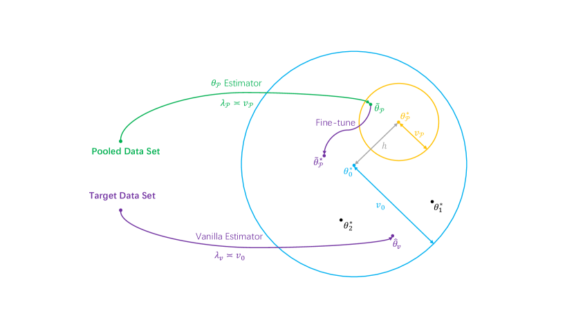
We take the seminal oracle transfer lasso algorithm for model (3) by Li et al., 2022a as an example and provide visualization in Figure 3 for better illustration. For the target parameter $\bm{\theta}^{*}_{0}$ colored in blue and informative source parameters colored in black, recall that Li et al., 2022a introduce the population version of $\widehat{\bm{\theta}}_{{\mathcal{P}}}$ as $\bm{\theta}^{*}_{\mathcal{P}}=\mathop{\text{\rm arg\,min}}\sum_{k\in\mathcal{P}}n_{k}{\mathbb{E}}[\mathcal{L}_{k}(\bm{Z}_{k};\bm{\theta})]/n_{\mathcal{P}}$, by setting $n_{\mathcal{P}}=\sum_{k\in{\mathcal{P}}}n_{k}$ and $\mathcal{L}_{k}$ as the least square loss. Under sparse contrast vectors and homogeneous Hessians of the loss functions (population covariance matrices of designs in this case), $\bm{\theta}^{*}_{\mathcal{P}}$ would be close to $\bm{\theta}^{*}_{0}$ if all $\bm{\theta}^{*}_{k}$ are, in the sense of sparsity measured by $h$. For $v_{\mathcal{P}}\asymp(\log p/n_{{\mathcal{P}}})^{1/2}$, Li et al., 2022a first estimate $\bm{\theta}^{*}_{\mathcal{P}}$ by equation (5) with tuning parameter $\lambda_{\mathcal{P}}\asymp v_{\mathcal{P}}$, acquiring $\widetilde{\bm{\theta}}_{\mathcal{P}}$. In the second step, they plug-in $\widetilde{\bm{\theta}}_{\mathcal{P}}$ and estimate $\bm{\theta}^{*}_{0}-\bm{\theta}^{*}_{\mathcal{P}}$ by equation (7). The resulting estimator, achieving min-max lower bound, outperforms the vanilla estimator $\widehat{\bm{\theta}}_{v}$ colored in purple with the error rate $v_{0}\asymp(\log p/n_{0})^{1/2}$, if the bias $h$ is small enough.

Refer to caption
Figure 3: Oracle transfer learning under individual contrasts with low-dimensional structures and homogeneous Hessians of loss functions.

Unfortunately, this framework fails to explain the role of fine-tuning if the individual contrast vectors have no low-dimensional structure in nature as under the settings of Figures 1 and 2. Moreover, even if the individual sparsity does exist, the problem gets complicated as the designs deviate even slightly from being homogeneous, as shown by the following example.

Example 2.1 (Oracle transfer lasso under almost homogeneous designs).

For independent $\bm{X}_{k,i}$ such that ${\mathbb{E}}\bm{X}_{k,i}=0$, $\bm{\Sigma}_{k}={\mathbb{E}}\bm{X}_{k,i}\bm{X}_{k,i}^{\top}$ and independent noise $\varepsilon_{k,i}\sim N(0,\bm{I}_{p})$, let $y_{k,i}=\langle\bm{\theta}^{*}_{k},\bm{X}_{k,i}\rangle+\varepsilon_{k,i}$, $k=0,1,2$. In addition, assume that $n_{0}=n_{1}=n_{2}$, $\bm{\theta}^{*}_{0}$ is $s$-sparse. It is shown in Li et al., 2022a that for $\bm{\delta}^{*}_{k}=\bm{\theta}^{*}_{0}-\bm{\theta}^{*}_{k}$, we have

$$\bm{\theta}^{*}_{0}-\bm{\theta}^{*}_{\mathcal{P}}=\left(\sum_{k=0}^{2}\bm{\Sigma}_{k}\right)^{-1}\left(\bm{\Sigma}_{1}\bm{\delta}_{1}+\bm{\Sigma}_{2}\bm{\delta}_{2}\right).$$

As for homogeneous designs such that the covariance matrices are set as $\bm{\Sigma}_{0}=\bm{\Sigma}_{1}=\bm{\Sigma}_{2}$, we have $\bm{\theta}^{*}_{0}-\bm{\theta}^{*}_{\mathcal{P}}\asymp(\bm{\delta}_{1}+\bm{\delta}_{2})$, which should be well-bounded by $\|\cdot\|_{1}$ by triangular inequality once we assume $\|\bm{\delta}^{*}_{k}\|_{1}\leq h$. However, consider the almost-homogeneous designs such that

$$\bm{\Sigma}_{0}=\bm{I}_{p},\quad\bm{\Sigma}_{1}=\bm{I}_{p}+c\bm{Z}_{p},\quad\bm{\Sigma}_{2}=\bm{I}_{p}-c\bm{Z}_{p},$$

where $\bm{Z}_{p}$ is a fixed realization from the standard Gaussian orthogonal ensemble (GOE), which is the symmetric random matrix with the diagonal elements taken independently from $N(0,2p^{-1})$ and the off-diagonal ones taken independently from $N(0,p^{-1})$. As $p\rightarrow\infty$, the spectrum of $\bm{Z}_{p}$ is bounded within $[-2,2]$ with high probability, so $\bm{\Sigma}_{1}$ and $\bm{\Sigma}_{2}$ are positive definite with high probability for sufficiently small $c>0$. Notably, $\|{\mathop{\text{\rm vec}}}(\bm{\Sigma}_{1})-{\mathop{\text{\rm vec}}}(\bm{\Sigma}_{2})\|_{\infty}\asymp\|{\mathop{\text{\rm vec}}}(\bm{Z}_{p})\|_{\infty}\lesssim(\log p/p)^{1/2}\rightarrow 0$ as $p\rightarrow\infty$. In this case, we have $\bm{\theta}^{*}_{0}-\bm{\theta}^{*}_{\mathcal{P}}\asymp(\bm{\delta}_{1}+\bm{\delta}_{2})+c\bm{Z}_{p}(\bm{\delta}_{1}-\bm{\delta}_{2})$. Let $\bm{\delta}_{1}=-\bm{\delta}_{2}=(h,0,\cdots,0)^{\top}$, $\bm{Z}_{p}=(\bm{z}_{1},\bm{z}_{2},\cdots,\bm{z}_{p})$, we have

$$\|\bm{\theta}^{*}_{0}-\bm{\theta}^{*}_{\mathcal{P}}\|_{1}\asymp ch\|\bm{z}_{1}\|_{1}\gtrsim ch\sqrt{p}\rightarrow\infty,$$

by observing that $\|\bm{z}_{1}\|_{1}$ approximately equals to sum of $p$ independent absolute value of $N(0,p^{-1})$.

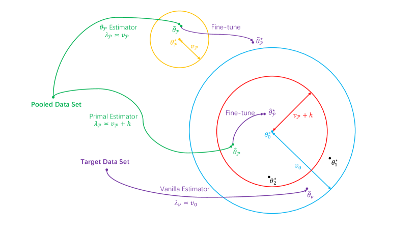
That is to say, the population pooling parameter $\bm{\theta}^{*}_{\mathcal{P}}$ could be really far away from $\bm{\theta}^{*}_{0}$ even if all $\bm{\theta}^{*}_{k}$ are close, in the sense of sparsity, under heterogeneous designs as illustrated by Figure 4. Not to mention the impracticability of sparse individual contrasts in the first place. Then, transfer learning would have little use if one has the intention of correctly estimating $\bm{\theta}^{*}_{\mathcal{P}}$ in the pooling step. On the other hand, for $\mathcal{B}_{k}(\bm{\delta}^{*}_{k})\leq h$, $\mathcal{B}_{k}$ can be the vector $\ell_{1}$ or $\ell_{2}$ norm for example, if we instead impose the slightly stronger regularization $\lambda_{\mathcal{P}}\asymp(h+v_{\mathcal{P}})$ (could be viewed as the combination of bias and variance) for pooling, then under the settings of Example 2.1, with high probability,

$$\|\widehat{\bm{\theta}}_{\mathcal{P}}-\bm{\theta}^{*}_{0}\|_{1}\lesssim s\left[h+(\log p/n_{{\mathcal{P}}})^{1/2}\right].$$

In this case, $\widehat{\bm{\theta}}_{\mathcal{P}}$ might be a terrible estimator of $\bm{\theta}^{*}_{\mathcal{P}}$, but it contains more information of $\bm{\theta}^{*}_{0}$ than $\widetilde{\bm{\theta}}_{\mathcal{P}}$, and is therefore a better primal estimator for the fine-tuning step.

Refer to caption
Figure 4: Oracle transfer learning under individual contrasts without low-dimensional structures or heterogeneous Hessians of loss functions.

2.3 Unknown Informative Auxiliary Samples

To avoid negative transfer when the informative sources are unknown, we propose a truncated-penalized algorithm to obtain a primal estimator in the first step, with the intuition of dataset clustering. For each dataset ${\mathbb{D}}_{k}$, $k=0,\cdots,K$, with the population parameter $\bm{\theta}^{*}_{k}$, let $\bm{\Theta}=\left(\bm{\theta}_{0},\cdots,\bm{\theta}_{K}\right)$, $\widehat{\bm{\Theta}}=\left(\widehat{\bm{\theta}}_{0},\cdots,\widehat{\bm{\theta}}_{K}\right)\in{\mathbb{R}}^{p\times(K+1)}$, consider the following non-convex problem with weights $(\alpha_{0},\cdots,\alpha_{K})$ given in advance:

$$\widehat{\bm{\Theta}}=\mathop{\text{\rm arg\,min}}_{\bm{\Theta}\in{\mathbb{R}}^{p\times(K+1)}}\sum_{k=0}^{K}\sum_{i=1}^{n_{k}}\frac{\alpha_{k}}{N}\mathcal{L}_{k}\left(\bm{Z}_{k,i};\bm{\theta}_{k}\right)+\sum_{k=0}^{K}\frac{n_{k}\lambda_{\mathcal{P}}}{N}{\mathcal{R}}\left(\bm{\theta}_{k}\right)+\sum_{k=1}^{K}\frac{n_{k}\lambda_{\mathcal{Q}_{k}}}{N}\mathcal{Q}\left(\bm{\theta}_{k}-\bm{\theta}_{0}\right),$$ (8)

where $N=\sum_{k=0}^{K}n_{k}$ and $\mathcal{Q}(\cdot)=\min\left[\mathcal{R}(\cdot),\tau\right]$ is the truncated norm penalty for some $\tau>0$. Then $\widehat{\bm{\theta}}_{0}$ is set to be the primal estimator.

Algorithm 2 Transfer learning for M-estimators with useful dataset selection.
0:    the target dataset ${\mathbb{D}}_{0}$ and arbitrary source datasets ${\mathbb{D}}_{k}$, $k=1,\cdots,K$;tuning parameters: weights $(\alpha_{k})_{k=0}^{K}$; $\lambda_{\mathcal{P}}$, $(\lambda_{\mathcal{Q}_{k}})_{k=1}^{K}$ and $\tau$; $l_{\mathcal{P}}$ (or $\lambda_{d}$);
0:    
1:  acquire the primal estimator $\widehat{\bm{\theta}}_{0}$ by taking the first column of $\widehat{\bm{\Theta}}$, the solution of (8);
2:  plug in the primal estimator $\widehat{\bm{\theta}}_{0}$ to acquire the fine-tuned estimator $\widehat{\bm{\theta}}^{\star}_{\mathcal{P}}$ according to the constrained problem (6) or the Lagrangian form (7);
3:  return  $\widehat{\bm{\theta}}^{\star}_{0}$.

The tuning parameter $\lambda_{\mathcal{Q}_{k}}$ controls the strength of dataset clustering. If $\lambda_{\mathcal{Q}_{k}}=0$, then (8) calculates each $\widehat{\bm{\theta}}_{k}$ using ${\mathbb{D}}_{k}$ alone with penalty $\mathcal{R}$ and tuning parameter $\lambda_{\mathcal{P}}$. On the other hand, if $\lambda_{\mathcal{Q}_{k}}\rightarrow\infty$, then optimization problem (8) is equivalent to the optimization problem (5) by blind-pooling all the sources and the target dataset.

If the individual contrast $\bm{\delta}^{*}_{k}=\bm{\theta}^{*}_{0}-\bm{\theta}^{*}_{k}$ has certain low-dimensional structure (e.g., sparsity), for some properly chosen $\lambda_{\mathcal{Q}_{k}}$ and $\tau$, problem (8) is in the same spirit of the one proposed by Li et al., (2023) such that the target parameter $\bm{\theta}^{*}_{0}$ and contrast vectors $\bm{\delta}^{*}_{k}$ are estimated simultaneously. On the other hand, if $\bm{\delta}^{*}_{k}$ has no such structure but still small as measured by $\mathcal{B}_{k}$, the decomposable regularizer $\mathcal{R}$ in $\mathcal{Q}$ tends to penalize $\widehat{\bm{\theta}}_{0}-\widehat{\bm{\theta}}_{k}$ towards zero. In the end, note that (8) possesses the dataset selection capability as those non-informative datasets ${\mathbb{D}}_{k}$, identified by $\mathcal{R}(\widehat{\bm{\theta}}_{0}-\widehat{\bm{\theta}}_{k})>\tau$, would have no influence on the estimator $\widehat{\bm{\theta}}_{0}$ due to the truncation in $\mathcal{Q}$.

To numerically solve problem (8) which is non-convex in nature, we adopt the modified difference of convex (DC) programming with the alternating direction method of multipliers (ADMM) procedures (Boyd et al.,, 2011; Wu et al.,, 2016; Fan et al., 2019a, ; Fan et al., 2019b, ; Fan et al.,, 2021). We defer the algorithm details under specific statistical models to Section 4.

3 Statistical Theory

In this section, we first focus on the statistical theories for oracle two-step transfer learning under a general framework. In Section 3.2 we discuss detailed statistical models under the framework. Then, theoretical analysis concerning the truncated-penalized algorithm is presented in Section 3.3.

3.1 Oracle Transfer Learning

Given all useful source datasets and the corresponding observations $\{\bm{Z}_{k,i}\}^{k\in\mathcal{P}}_{1\leq i\leq n_{k}}$ generated from certain probabilistic model, we discuss the role of the pooling and the fine-tuning of Algorithm 1, respectively.

3.1.1 The Role of Pooling

We first consider the deterministic functions $\bm{L}_{k}(\bm{\theta})=\sum_{1\leq i\leq n_{k}}\mathcal{L}_{k}(\bm{Z}_{k,i};\bm{\theta})/n_{k}$, $k=0,\cdots K$. By setting $\alpha_{k}=1$, optimization problem (5) can be rewritten as

$$\widehat{\bm{\theta}}_{\mathcal{P}}=\mathop{\text{\rm arg\,min}}_{\bm{\theta}\in{\mathbb{R}}^{p}}\bm{L}_{\mathcal{P}}(\bm{\theta})+\lambda_{\mathcal{P}}\mathcal{R}(\bm{\theta}),$$

where $\bm{L}_{\mathcal{P}}=\sum_{k\in\mathcal{P}}n_{k}\bm{L}_{k}/n_{\mathcal{P}}$ and $n_{\mathcal{P}}=\sum_{k\in\mathcal{P}}n_{k}$. We first introduce some useful notations from Negahban et al., (2012), recall that the regularizer $\mathcal{R}$ is decomposable with respect to $(\mathcal{M},\overline{\mathcal{M}}^{\perp})$ such that $\bm{\theta}^{*}_{0}\in\mathcal{M}\subset\overline{\mathcal{M}}$. Let ${\mathcal{R}}^{*}(\bm{v})=\sup_{{\mathcal{R}}(\bm{u})\leq 1}\langle\bm{u},\bm{v}\rangle$ be the dual norm of ${\mathcal{R}}$, define

$$\delta\bm{L}(\bm{\Delta};\bm{\theta}^{*}_{0})=\bm{L}(\bm{\theta}^{*}_{0}+\bm{\Delta})-\bm{L}(\bm{\theta}^{*}_{0})-\left\langle\nabla\bm{L}(\bm{\theta}^{*}_{0}),\bm{\Delta}\right\rangle,$$

and $\Psi({\mathcal{M}})=\sup_{\bm{u}\in{\mathcal{M}}\backslash\{0\}}{\mathcal{R}}(\bm{u})/\|\bm{u}\|$ is the subspace compatibility constant. In the end, define the cone-like set

$${\mathbb{C}}\left(\mathcal{M},\overline{\mathcal{M}}^{\perp};\bm{\theta}^{*}\right):=\left\{\bm{\Delta}\in\mathbb{R}^{p}\mid\mathcal{R}\left(\bm{\Delta}_{\overline{\mathcal{M}}^{\perp}}\right)\leq 3\mathcal{R}\left(\bm{\Delta}_{\overline{\mathcal{M}}}\right)+4{\mathcal{R}}(\bm{\theta}^{*}_{{\mathcal{M}}^{\perp}})\right\},$$

where the subscript, e.g., $\bm{\Delta}_{\overline{\mathcal{M}}}$ means the projection of $\bm{\Delta}$ onto the subspace $\overline{\mathcal{M}}$. We first present the role of pooling by the following lemma.

Lemma 1 (Primal information).

Under the settings of this section, consider the problem (5) with $\lambda_{\mathcal{P}}\geq 2{\mathcal{R}}^{*}\left(\nabla\bm{L}_{\mathcal{P}}(\bm{\theta}^{*}_{0})\right)$, suppose $\bm{L}_{\mathcal{P}}$ is convex, differentiable and satisfies the restricted strong convexity (RSC) condition:

$$\delta\bm{L}_{\mathcal{P}}(\bm{\Delta};\bm{\theta}^{*}_{0})\geq\kappa_{\mathcal{P}}\|\bm{\Delta}\|^{2}-\tau_{\mathcal{P}},\quad\text{for all }\bm{\Delta}\in\mathbb{C}\left(\mathcal{M},\overline{\mathcal{M}}^{\perp};\bm{\theta}^{*}_{0}\right),$$ (9)

with $\tau_{\mathcal{P}}\lesssim\lambda_{\mathcal{P}}\Psi^{2}(\overline{\mathcal{M}})/\kappa_{\mathcal{P}}$, we have the following bounds:

$$\|\widehat{\bm{\theta}}_{\mathcal{P}}-\bm{\theta}^{*}_{0}\|^{2}\lesssim\frac{\lambda^{2}_{\mathcal{P}}}{\kappa^{2}_{\mathcal{P}}}\Psi^{2}(\overline{\mathcal{M}}),\quad\mathcal{R}(\widehat{\bm{\theta}}_{\mathcal{P}}-\bm{\theta}^{*}_{0})\lesssim\frac{\lambda_{\mathcal{P}}}{\kappa_{\mathcal{P}}}\Psi^{2}(\overline{\mathcal{M}}).$$ (10)

As clarified in Negahban et al., (2012), we require the restricted strong convexity condition only on the intersection of $\mathbb{C}$ with a local ball $\{\|\bm{\Delta}\|\leq R\}$, where $R$ is the error radius. Such intersection is not necessary for the least-squares loss with quadratic error, but is essential for general loss functions such as those in generalized linear models.

We then take a closer look at the rate term ${\mathcal{R}}^{*}\left(\nabla\bm{L}_{\mathcal{P}}(\bm{\theta}^{*}_{0})\right)$. Assume that all $\bm{L}_{k}$ have the second-order derivative at $\bm{\theta}^{*}_{k}$, let $\bm{\delta}^{*}_{k}=\bm{\theta}^{*}_{0}-\bm{\theta}^{*}_{k}$, by Taylor expansion and triangular inequality,

$\displaystyle\mathcal{R}^{*}\left(\nabla\bm{L}_{\mathcal{P}}(\bm{\theta}^{*}_{0})\right)$ $\displaystyle=\mathcal{R}^{*}\left(\sum_{k\in\mathcal{P}}n_{k}\left[\nabla\bm{L}_{k}(\bm{\theta}^{*}_{k})+\nabla^{2}\bm{L}_{k}(\bm{\theta}^{*}_{0})\bm{\delta}^{*}_{k}+\bm{r}_{k}(\bm{\delta}^{*}_{k})\right]\right)/n_{\mathcal{P}}$ (11)
$\displaystyle\leq\underbrace{\mathcal{R}^{*}\left(\sum_{k\in\mathcal{P}}n_{k}\nabla\bm{L}_{k}(\bm{\theta}^{*}_{k})\right)/n_{\mathcal{P}}}_{v_{\mathcal{P}}}+\underbrace{\sum_{k\in\mathcal{P}}n_{k}{\mathcal{R}}^{*}\left(\nabla^{2}\bm{L}_{k}(\bm{\theta}^{*}_{k})\bm{\delta}^{*}_{k}\right)/n_{\mathcal{P}}}_{b_{\mathcal{P}}}$
$\displaystyle\quad+\underbrace{\mathcal{R}^{*}\left(\sum_{k\in\mathcal{P}}n_{k}\bm{r}_{k}(\bm{\delta}^{*}_{k})\right)/n_{\mathcal{P}}}_{\text{remainder}}.$

For sufficiently small $\bm{\delta}^{*}_{k}$, the remainder could be absorbed into the first two terms. Since $\bm{\theta}^{*}_{k}$ are assumed to be the minimizers of population loss functions, which means ${\mathbb{E}}\nabla\bm{L}_{k}(\bm{\theta}^{*}_{k})=0$. The first term $v_{\mathcal{P}}$ could be viewed as the variance term, and is often well-controlled by standard high-dimensional probabilistic arguments, proportional to $n_{\mathcal{P}}^{-1/2}$. The second term $b_{\mathcal{P}}$ could be viewed as the bias term and is the origin of the regularization enlargement. Define the $(\mathcal{B}_{k}$,$\mathcal{R}^{*})$-operator norm of the $m\times n$ matrix $\bm{A}=(\bm{A}_{1},\cdots,\bm{A}_{n})$ by

$$\|\bm{A}\|_{\mathcal{B}_{k}\rightarrow\mathcal{R}^{*}}=\sup_{\mathcal{B}_{k}(\bm{v})\leq 1}\mathcal{R}^{*}\left(\bm{A}\bm{v}\right),$$

where $A_{j}$ is the $j$-th column of $\bm{A}$. We claim $b_{\mathcal{P}}\lesssim h$ as long as $\mathcal{B}_{k}(\bm{\delta}^{*}_{k})\leq h$ and $\|\nabla^{2}\bm{L}_{k}(\bm{\theta}^{*}_{k})\|_{\mathcal{B}_{k}\rightarrow\mathcal{R}^{*}}$ can be bounded by some constants.

Indeed, the matrix operator norms are not equivalent as dimension $p\rightarrow\infty$ (Lewis,, 2010). Now, let’s go back to Example 2.1 and get some intuition on the chance for $\|\bm{\theta}^{*}_{0}-\widehat{\bm{\theta}}_{\mathcal{P}}\|_{1}$ being small while $\|\bm{\theta}^{*}_{0}-\bm{\theta}^{*}_{\mathcal{P}}\|_{1}$ being really large in the case of sparse linear regression, from the aspect of matrix operator norms. In Example 2.1 where $\|\bm{\delta}^{*}_{k}\|_{1}\leq h$, $\|\bm{\theta}^{*}_{0}-\bm{\theta}^{*}_{\mathcal{P}}\|_{1}$ is dominated by $\|\bm{\Sigma}_{k}\bm{\delta}^{*}_{k}\|_{1}$, while the bias term of $\|\bm{\theta}^{*}_{0}-\widehat{\bm{\theta}}_{\mathcal{P}}\|_{1}$, as shown here, is dominated by $\|\widehat{\bm{\Sigma}}_{k}\bm{\delta}^{*}_{k}\|_{\infty}$. Here $\bm{\Sigma}_{k}$, $\widehat{\bm{\Sigma}}_{k}$ are the population and sample covariance matrices of the $n_{k}\times p$ design matrix $\mathbf{\mathcal{X}}_{k}=\left(\bm{X}_{k,1},\dots,\bm{X}_{k,n_{k}}\right)^{\top}$, respectively. Now, given matrix $\bm{A}$, we have

$$\|\bm{A}\|_{1\rightarrow 1}=\sup_{\|\bm{v}\|_{1}\leq 1}\|\bm{A}\bm{v}\|_{1}=\max_{j=1,\ldots,n}\left\|\bm{A}_{j}\right\|_{1},$$
$$\|\bm{A}\|_{1\rightarrow\infty}=\sup_{\|\bm{v}\|_{1}\leq 1}\|\bm{A}\bm{v}\|_{\infty}=\max_{j=1,\ldots,n}\left\|\bm{A}_{j}\right\|_{\infty}.$$

It is easy to verify that $\|\widehat{\bm{\Sigma}}_{k}\|_{1\rightarrow\infty}\ll\|\bm{\Sigma}_{k}\|_{1\rightarrow 1}$ holds in most cases for sufficiently large dimension $p$, and $\|\bm{\theta}^{*}_{0}-\widehat{\bm{\theta}}_{\mathcal{P}}\|_{1}$ is much easier to be upper-bounded than $\|\bm{\theta}^{*}_{0}-\bm{\theta}^{*}_{\mathcal{P}}\|_{1}$ in these cases.

Meanwhile, one could also assume $\|\bm{\delta}^{*}_{k}\|_{2}\leq h$, note that for $\bm{A}^{\top}=\left((\bm{A}^{\top})_{1},\cdots,(\bm{A}^{\top})_{m}\right)$,

$$\|\bm{A}\|_{2\rightarrow\infty}=\sup_{\|\bm{v}\|_{2}\leq 1}\|\bm{A}\bm{v}\|_{\infty}=\max_{i=1,\ldots,m}\left\|(\bm{A}^{\top})_{i}\right\|_{2},$$

where $(\bm{A}^{\top})_{i}$ is the $i$-th column of $\bm{A}^{\top}$. It is easy to verify that $\|\bm{A}\|_{2\rightarrow\infty}\leq\|\bm{A}\|_{\text{op}}$, so that $\|\widehat{\bm{\Sigma}}_{k}\|_{2\rightarrow\infty}$ is well-bounded by the largest eigenvalue of $\widehat{\bm{\Sigma}}_{k}$. According to the random matrix theory (Yin et al.,, 1988; Bai and Silverstein,, 1998, 2010), for the $n_{k}\times p$ design matrix $\mathbf{\mathcal{X}}_{k}$, as long as the dimension $p$ is not too large in a sense that $p/n_{k}\rightarrow c_{k}\in(0,\infty)$, while the underlying distribution is not too heavy-tailed, e.g., has finite fourth moment, it holds that the largest eigenvalue of $\widehat{\bm{\Sigma}}_{k}$ tends to a finite limit, depending only on $c_{k}$ and the population covariance matrix $\bm{\Sigma}_{k}$, almost surely. Hence, as demonstrated in Figure 1, those source datasets with non-sparse contrast vectors with small $\ell_{2}$ norm are also beneficial for the pooling step under mild conditions.

3.1.2 The Role of Fine-tuning

According to equation (10) in Lemma 1, we have ${\mathcal{R}}(\widehat{\bm{\theta}}_{\mathcal{P}}-\bm{\theta}^{*}_{0})\leq l_{{\mathcal{P}}}$ for some $l_{\mathcal{P}}\asymp\lambda_{\mathcal{P}}\Psi^{2}(\overline{\mathcal{M}})/\kappa_{\mathcal{P}}$. We then show how such information enhances performance via fine-tuning the estimators from the constrained optimization (6) or the Lagrangian version in equation (7) . Again we use $\widehat{\bm{\theta}}^{\star}_{\mathcal{P}}$, $l_{\mathcal{P}}$, $\lambda_{d}$, $\kappa_{d}$ and $\tau_{d}$ in both problems with a slight abuse of notations.

Theorem 1 (Oracle transfer learning).

Given the primal estimator $\widehat{\bm{\theta}}_{\mathcal{P}}$ satisfying ${\mathcal{R}}(\widehat{\bm{\theta}}_{\mathcal{P}}-\bm{\theta}^{*}_{0})\leq l_{{\mathcal{P}}}$ for some $l_{\mathcal{P}}\asymp\lambda_{\mathcal{P}}\Psi^{2}(\overline{\mathcal{M}})/\kappa_{\mathcal{P}}$. Take $\lambda_{d}\gtrsim R^{*}(\nabla\bm{L}_{0}(\bm{\theta}^{*}_{0}))$, assume that $\bm{L}_{0}$ is convex, differentiable and satisfies the restricted strong convexity (RSC) condition:

$$\delta\bm{L}_{0}(\bm{\Delta};\bm{\theta}^{*}_{0})\geq\kappa_{d}\|\bm{\Delta}\|^{2}-\tau_{d},\quad\text{for all }\mathcal{R}(\bm{\Delta})\leq 4l_{\mathcal{P}},$$ (12)

with $\tau_{d}\lesssim\lambda_{d}l_{\mathcal{P}}$. The constrained problem (6) using $l_{\mathcal{P}}$ (or the Lagrangian problem (7) using $\lambda_{d}$) would result in the transfer learning estimator which satisfies

$$\|\widehat{\bm{\theta}}^{\star}_{\mathcal{P}}-\bm{\theta}^{*}_{0}\|^{2}\lesssim\frac{\lambda_{\mathcal{P}}\lambda_{d}\Psi^{2}(\overline{\mathcal{M}})}{\kappa_{\mathcal{P}}\kappa_{d}}.$$

Note that the vanilla estimator using only target data satisfies $\|\widehat{\bm{\theta}}_{v}-\bm{\theta}^{*}_{0}\|^{2}\lesssim\lambda_{d}^{2}$. To make knowledge transfer from the source datasets preferable, we need $\lambda_{\mathcal{P}}\lesssim\lambda_{d}$, where $\lambda_{\mathcal{P}}$ is closely related to the variance and bias of the pooled datasets as shown by equation (11). In the end, recall that the pooling estimator without fine-tuning satisfies $\|\widehat{\bm{\theta}}_{\mathcal{P}}-\bm{\theta}^{*}_{0}\|^{2}\lesssim\lambda_{\mathcal{P}}^{2}$ according to equation (10). If $v_{\mathcal{P}}$ and $b_{\mathcal{P}}$ are so small that $\lambda_{\mathcal{P}}\ll\lambda_{d}$, then the fine-tuning step is unnecessary as it only introduces additional variance from the target dataset. As shown in Figures 1 and 2, the fine-tuned estimators dominate only when the contrasts are neither too big or too small in $\ell_{2}$ norm. In short, knowledge transfer is favorable as long as the biases of the source datasets are smaller than the original target variance, but the fine-tuning step should only be considered when the biases are also not too small. Hence cross validation is suggested when choosing the tuning parameter of the fine-tuning step in practice.

3.2 Specific Statistical Models

We then focus on detailed statistical models under the framework, including the sparse linear regression in Section 3.2.1 and the generalized low-rank trace regression in Section 3.2.2.

3.2.1 Sparse Linear Regression

First, we assume the datasets are generated from the linear model $y_{k,i}=\langle\bm{\theta}^{*}_{k},\bm{X}_{k,i}\rangle+\varepsilon_{k,i}$ for $i=1,\dots,n_{k}$ and $k=0,\dots,K$. Let $\bm{\theta}^{*}_{0}$ be $s$-sparse with $s<\infty$. To cope with the sparsity structure of $\bm{\theta}^{*}_{0}$, we take the decomposable regularizer $\mathcal{R}=\|\cdot\|_{1}$. For simplicity, we follow Raskutti et al., (2010) and assume that the $n_{k}\times p$ design matrices $\mathbf{\mathcal{X}}_{k}=\left(\bm{X}_{k,1},\dots,\bm{X}_{k,n_{k}}\right)^{\top}$ are formed by independently sampling $n_{k}$ identical $\bm{X}_{k,i}\sim N(0,\bm{\Sigma}_{k})$ with the covariance matrices $\bm{\Sigma}_{k}$ satisfying $M_{1}^{-1}\leq\lambda_{\min}(\bm{\Sigma}_{k})\leq\lambda_{\max}(\bm{\Sigma}_{k})\leq M_{1}$, which is referred to as the $\bm{\Sigma}_{k}$-Gaussian ensembles. In addition, assume that $\varepsilon_{k,i}$ are independently drawn from the same centered sub-Gaussian distribution. For $k=1,\dots,K$, we assume either $\|\bm{\delta}^{*}_{k}\|_{1}\leq h$ or $\|\bm{\delta}^{*}_{k}\|_{2}\leq h$ for $\bm{\delta}^{*}_{k}=\bm{\theta}^{*}_{0}-\bm{\theta}^{*}_{k}$. In the end, we set $\alpha_{k}=1$ for all $k\in\mathcal{P}$.

Theorem 2 (Sparse linear regression).

Under the settings of this section, we set $\lambda_{\mathcal{P}}\asymp\left[(\log p/n_{\mathcal{P}})^{1/2}+h\right]$ in the pooling step, and $l_{\mathcal{P}}\asymp s\lambda_{\mathcal{P}}$ for the constrained problem (or $\lambda_{d}\asymp(\log p/n_{0})^{1/2}$ for the Lagrangian problem). Assume that $\log p\lesssim n_{0}$, as $\min_{k\in\mathcal{P}}n_{k}\rightarrow\infty$, $p\rightarrow\infty$ with $\log p/n_{\mathcal{P}}\rightarrow 0$ (if $\|\bm{\delta}^{*}_{k}\|_{2}\leq h$, we further assume that $p/n_{k}\rightarrow c_{k}$ for some positive constant $c_{k}$) and $h\rightarrow 0$, we have the oracle pooling and fine-tuned estimators satisfy

$$\|\widehat{\bm{\theta}}_{\mathcal{P}}-\bm{\theta}^{*}_{0}\|^{2}=O_{p}\left[\frac{\log p}{n_{\mathcal{P}}}+h^{2}\right],\quad\|\widehat{\bm{\theta}}^{\star}_{\mathcal{P}}-\bm{\theta}^{*}_{0}\|^{2}=O_{p}\left[\sqrt{\frac{\log p}{n_{0}}}\left(\sqrt{\frac{\log p}{n_{\mathcal{P}}}}+h\right)\right].$$

We report simultaneously the rate of the oracle pooling estimator $\widehat{\bm{\theta}}_{\mathcal{P}}$ and the fine-tuned estimator $\widehat{\bm{\theta}}^{\star}_{\mathcal{P}}$ with the intention of emphasizing the regime suitable for fine-tuning. Indeed, if $h\ll(\log p/n_{0})^{1/2}$, introducing the target dataset for the second step tends to be harmful, as also alluded in Figure 1. Furthermore, the gain by fine-tuning is slightly smaller than the improvement from estimating a sparse difference vector, i.e., debiasing, as in Li et al., 2022a . The latter has the convergence rate of $(\log p/n_{\mathcal{P}})+h(\log p/n_{0})^{1/2}$. However, as also shown later by the numerical simulation, the fine-tuning step is able to work without the contrasts’ low-dimensional structure and homogeneous Hessians of loss functions, while the ideology of debiasing is very sensitive to those assumptions.

3.2.2 Generalized Low-rank Trace Regression

As for generalized low-rank trace regression, let $\mathcal{D}_{k}$ consist of $n_{k}$ i.i.d. samples of $\bm{Z}_{k,i}=(\bm{X}_{k,i},y_{k,i})$, where ${\mathbb{P}}(y_{k,i}|\bm{X}_{k,i})\propto\exp\left\{y_{k,i}\eta_{k,i}-b_{k}(\eta_{k,i})\right\}$ for $\eta_{k,i}=\langle\bm{\theta}^{*}_{k},\bm{X}_{k,i}\rangle$. Assume $\bm{\theta}^{*}_{0}$ is of rank $r$ with $r<\infty$. Recall the subspaces defined in equations (1), (2) and we take $\mathcal{R}=\|\cdot\|_{N}$ as the decomposable regularizer. For brevity, we follow Fan et al., 2019a and assume $\bm{\theta}^{*}_{k}$ to be $d\times d$ square matrices. All analysis could be extended readily to rectangular cases of dimensions $d_{1}\times d_{2}$, with the rate replaced by $d=\max(d_{1},d_{2})$. In addition, assume all datasets share the same $b_{k}(\cdot)=b(\cdot)$ and set $\alpha_{k}=1$, where $b^{\prime}\left(\eta_{k,i}\right)={\mathbb{E}}\left(y_{k,i}|\bm{X}_{k,i}\right)$ is called the inverse link function, and $b^{\prime\prime}\left(\eta_{k,i}\right)=\text{Var}\left(y_{k,i}|\bm{X}_{k,i}\right)$. As also pointed out in Tian and Feng, (2022), using different $b_{k}$ is also allowed, but it is less practical. We take $\bm{L}_{k}(\bm{\theta})=\sum_{i\leq n_{k}}\left[-y_{k,i}\langle\bm{\theta},\bm{X}_{k,i}\rangle+b(\langle\bm{\theta},\bm{X}_{k,i}\rangle)\right]/n_{k}$, whose gradient and Hessian matrix are respectively

$$\nabla\bm{L}_{k}(\bm{\theta})=\frac{1}{n_{k}}\sum_{i\leq n_{k}}\left[b^{\prime}\left(\langle\bm{\theta},\bm{X}_{k,i}\rangle\right)-y_{k,i}\right]\bm{X}_{k,i},$$
$$\widehat{\bm{H}}_{k}(\bm{\theta}):=\nabla^{2}\bm{L}_{k}(\bm{\theta})=\frac{1}{n_{k}}\sum_{i\leq n_{k}}b^{\prime\prime}\left(\left\langle\bm{\theta},\bm{X}_{k,i}\right\rangle\right){\mathop{\text{\rm vec}}}\left(\bm{X}_{k,i}\right){\mathop{\text{\rm vec}}}\left(\bm{X}_{k,i}\right)^{\top}.$$

We make the following assumptions under the guidance of Fan et al., 2019a : (a) for each $k\in\mathcal{P}$, the vectorized version of $\bm{X}_{k,i}$ is taken independently from a sub-Gaussian random vector with bounded $\Psi_{2}$-norm, namely $\|{\mathop{\text{\rm vec}}}(\bm{X}_{k,i})\|_{\Psi_{2}}\leq M_{1}$; (b) we assume $|b^{\prime\prime}(\eta_{k,i})|\leq M_{2}$, $|b^{\prime\prime\prime}(\eta_{k,i})|\leq M_{3}$ almost surely; (c) let $\bm{H}_{k}(\bm{\theta}^{*}_{k})={\mathbb{E}}\widehat{\bm{H}}_{k}(\bm{\theta}^{*}_{k})$, assume that $\lambda_{\min}\left[\bm{H}_{k}(\bm{\theta}^{*}_{k})\right]\geq\kappa_{k}$; (d) we assume either $\|\bm{\delta}^{*}_{k}\|_{F}\leq h$, $\|\bm{\delta}^{*}_{k}\|_{N}\leq h$ or $\|{\mathop{\text{\rm vec}}}(\bm{\delta}^{*}_{k})\|_{1}\leq h$ for $\bm{\delta}^{*}_{k}=\bm{\theta}^{*}_{0}-\bm{\theta}^{*}_{k}$; (e) in the end, assume that $\|\bm{\theta}^{*}_{0}\|_{F}\geq\alpha\sqrt{d}$ for some constant $\alpha$. Then, we claim the following relative rate of convergence with respect to $\|\bm{\theta}^{*}_{0}\|^{2}_{F}$.

Theorem 3 (Generalized low-rank trace regression).

Under the settings of this section, we set $\lambda_{\mathcal{P}}\asymp d^{1/2}(n_{\mathcal{P}}^{-1/2}+h)$ in the first pooling step, $l_{\mathcal{P}}\asymp r\lambda_{\mathcal{P}}$ for the constrained problem (or $\lambda_{d}\asymp(d/n_{0})^{1/2}$ for the Lagrangian problem), assume $d\lesssim n_{0}$, as $n_{\mathcal{P}}\rightarrow\infty$, $d\rightarrow\infty$ and $h\rightarrow 0$ with $d^{1/2}(n_{\mathcal{P}}^{-1/2}+h)\rightarrow 0$, we have the oracle pooling and fine-tuned estimators satisfy

$$\frac{\|\widehat{\bm{\theta}}_{\mathcal{P}}-\bm{\theta}^{*}_{0}\|_{F}^{2}}{\|\bm{\theta}^{*}_{0}\|^{2}_{F}}=O_{p}\left[\frac{1}{n_{\mathcal{P}}}+h^{2}\right],\quad\frac{\|\widehat{\bm{\theta}}^{\star}_{\mathcal{P}}-\bm{\theta}^{*}_{0}\|_{F}^{2}}{\|\bm{\theta}^{*}_{0}\|^{2}_{F}}=O_{p}\left[\sqrt{\frac{1}{n_{0}}}\left(\sqrt{\frac{1}{n_{\mathcal{P}}}}+h\right)\right].$$

Most conditions here are taken directly from Fan et al., 2019a , except for (d) which is imposed for the transfer learning setting. We also point out that condition (b) is slightly stronger than that of Fan et al., 2019a . Indeed, (b) is automatically satisfied by the identity link $b^{\prime}(x)=x$ and the logit link $b^{\prime}(x)=1/(1+e^{-x})$. As for the inverse link $b^{\prime}(x)=x^{-1}$ and the inverse square link with $b^{\prime}(x)=x^{-1/2}$ where $b^{\prime\prime}(x)$ and $b^{\prime\prime\prime}(x)\rightarrow\infty$ as $x\rightarrow 0$, the condition (b) is to guarantee that $y_{k,i}$ does not have infinite variance, whereas Fan et al., 2019a require bounded $|b^{\prime\prime}(x)|$ for all $x\in{\mathbb{R}}$, $\left|b^{\prime\prime\prime}(x)\right|\leq|x|^{-1}$ for $|x|>1$ and sufficiently large $\eta_{k,i}$ with high probability.

Compared to the vanilla target estimator $\widehat{\bm{\theta}}_{v}$ with the relative convergence rate of $n_{0}^{-1}$ (Fan et al., 2019a, ), the oracle pooling and fine-tuned estimators have better performance if the difference $h$ is small enough. Similarly, fine-tuning should only be considered if $h$ is also not too small at the same time. In the end, we remark that under the framework of this paper, we only consider the role of fine-tuning for transfer generalized low-rank trace regression, while leaving the effect of estimating a difference vector with certain low-dimensional structure, i.e., debiasing, to the future work.

3.3 Oracle Property of the Truncated-Penalized Estimator

In the end of this section, we show that under mild conditions, $\widehat{\bm{\theta}}_{0}$ obtained from Algorithm 2 is as good as the oracle pooling estimator $\widehat{\bm{\theta}}_{\mathcal{P}}$ in terms of extracting primal information, which is referred to as the oracle property in this work. In fact, Theorem 1 allows plugging in any primal estimator that is sufficiently close to $\bm{\theta}^{*}_{0}$, it is easy to verify that the fine-tuned estimator $\widehat{\bm{\theta}}^{\star}_{0}$ is as good as $\widehat{\bm{\theta}}^{\star}_{\mathcal{P}}$ as well.

Theorem 4 (Oracle property of the truncated-penalized algorithm).

Let $\mathcal{A}$ denote the informative source datasets, and $\mathcal{A}^{c}$ denote the rest. For $k\in\mathcal{A}$, assume that $\mathcal{B}_{k}(\bm{\delta}^{*}_{k})\leq h$ and $\max(\|\nabla^{2}\bm{L}_{k}(\bm{\theta}^{*}_{k})\|_{\mathcal{R}\rightarrow\mathcal{R}^{*}},\|\nabla^{2}\bm{L}_{k}(\bm{\theta}^{*}_{k})\|_{\mathcal{B}_{k}\rightarrow\mathcal{R}^{*}})\leq M$. In addition, assume that conditions in Lemma 1 hold for $\mathcal{P}=\{0\}\cup\mathcal{A}$. As for $k\in\mathcal{A}^{c}$, define

$$\widehat{\bm{\theta}}^{\prime}_{k}=\mathop{\text{\rm arg\,min}}_{\bm{\theta}_{k}\in{\mathbb{R}}^{p}}\bm{L}_{k}\left(\bm{\theta}_{k}\right)+\lambda_{\mathcal{P}}{\mathcal{R}}\left(\bm{\theta}_{k}\right),$$

and assume that $\mathcal{R}(\widehat{\bm{\theta}}^{\prime}_{k}-\bm{\theta}^{*}_{0})>2\tau$ for some $\tau>0$. Denote $v_{k}=\mathcal{R}^{*}(\nabla\bm{L}_{k}(\bm{\theta}^{*}_{k}))$, for the optimization problem (8) with $\lambda_{\mathcal{P}}\gtrsim{\mathcal{R}}^{*}\left(\nabla\bm{L}_{\mathcal{P}}(\bm{\theta}^{*}_{0})\right)\asymp(v_{\mathcal{P}}+h)$ and $\lambda_{\mathcal{Q}_{k}}\gtrsim(v_{k}+h)$, as $\min_{k\in\mathcal{A}}n_{k}\rightarrow\infty$, $p\rightarrow\infty$ with $\max_{k\in\mathcal{A}}v_{k}<\infty$, $v_{\mathcal{P}}\rightarrow 0$ and $h\rightarrow 0$, there exists a local minimum $\widehat{\bm{\Theta}}$ whose first column satisfies:

$$\|\widehat{\bm{\theta}}_{0}-\bm{\theta}^{*}_{0}\|^{2}\lesssim\frac{\lambda^{2}_{\mathcal{P}}}{\kappa^{2}_{\mathcal{P}}}\Psi^{2}(\overline{\mathcal{M}}),\quad\mathcal{R}(\widehat{\bm{\theta}}_{0}-\bm{\theta}^{*}_{0})\lesssim\frac{\lambda_{\mathcal{P}}}{\kappa_{\mathcal{P}}}\Psi^{2}(\overline{\mathcal{M}}).$$

For $k\in\mathcal{A}$, the conditions in Theorem 4 are identical to those arguments in the oracle case. As for $k\in\mathcal{A}^{c}$, it might seem odd at first sight that we use the estimator $\widehat{\bm{\theta}}^{\prime}_{k}$ rather than the population value $\bm{\theta}^{*}_{k}$ in the assumption. However, note that $\widehat{\bm{\theta}}^{\prime}_{k}$ is exactly the primal estimator acquired by (5) using $\mathcal{D}_{k}$ alone, and $\mathcal{R}(\widehat{\bm{\theta}}^{\prime}_{k}-\bm{\theta}^{*}_{0})>2\tau$ essentially means that the dataset $\mathcal{D}_{k}$ is non-informative enough for $\bm{\theta}^{*}_{0}$ in this case. It eliminates those datasets with large sample sizes but large contrasts, and those with small contrasts but small sample sizes. It is worth mentioning that one might follow Li et al., (2023) and give an alternative rate of $\widehat{\bm{\theta}}_{0}$ under contrasts with low-dimensional structures by carefully choosing the strength of regularization. However, we do not pursue this direction but instead focus on the data selection capability of the truncated-penalized algorithm for contrasts potentially with no structure at all. In fact, as shown in Appendix C.3, the rates derived here are only different with those of Li et al., (2023) up to a comparable extent in the regime such that transfer learning is preferable, see detailed discussion therein.

4 Numerical Simulation

In section 4.1, we demonstrate numerically how slightly stronger regularization helps if either the low-dimensional structure of contrasts or the homogeneity of Hessian matrices is violated. Then, the truncated-penalized algorithm for detailed statistical models is discussed in section 4.2.

4.1 Slightly stronger regularization

As discussed in Section 2.2, the population parameter $\bm{\theta}^{*}_{\mathcal{P}}$ tends to be further away from $\bm{\theta}^{*}_{0}$ for contrast vectors without low-dimensional structure or heterogeneous Hessian matrices of loss functions. Here we focus on the sparse linear regression setting where $\bm{\theta}^{*}_{\mathcal{P}}$ admits a closed form solution (Li et al., 2022a, ; Tian and Feng,, 2022), and numerically verify that slightly stronger regularization benefits the oracle transfer learning case under certain settings.

We generate data from the linear model $y_{k,i}=\langle\bm{\theta}^{*}_{k},\bm{X}_{k,i}\rangle+\varepsilon_{k,i}$ for $i=1,\cdots,n_{k}$ and $k=0,\cdots,5$, where $\varepsilon_{k,i}$ is drawn independently from $N(0,1)$. For $\bm{X}_{k,i}$, we consider the following cases: (a) homogenous designs: draw $\bm{X}_{k,i}$ from $N(\bm{0},\bm{I}_{p})$ independently; (b) heterogeneous designs: for $k=0,1,\cdots,5$, let $\bm{\Lambda}_{k}$ be a matrix of $1.5p$ rows and $p$ columns whose elements are independently drawn from $N(0,1)$, then draw $\bm{X}_{k,i}$ independently from $N(\bm{0},\bm{\Sigma}_{k})$ with $\bm{\Sigma}_{k}=2\bm{\Lambda}_{k}^{\top}\bm{\Lambda}_{k}/(3p)$.

For $\bm{\theta}^{*}_{k}$, we consider two configurations. Let $s=0.04p$ and we set $\bm{\theta}^{*}_{0j}=0.4$ for $j\in[s]=\{1,\cdots,s\}$ where $\bm{\theta}^{*}_{kj}$ represents the $j$-th element of $\bm{\theta}^{*}_{k}$. Then we consider: (a) sparse contrasts: for each $k\in[5]$, let $H_{k}$ be a random subset of $[p]$ with $|H_{k}|=3$ and let $\bm{\theta}^{*}_{kj}=\bm{\theta}^{*}_{0j}-0.4I\left(\left\{j\in H_{k}\right\}\cap\left\{j\neq 1\right\}\right)$, $\bm{\theta}^{*}_{k1}=-0.4$; (b) dense contrasts: for each $k\in[5]$, let $H_{k}$ be a random subset of $[p]$ with $|H_{k}|=p/2$ and let $\bm{\theta}^{*}_{kj}=\bm{\theta}^{*}_{0j}+\xi_{j}I(j\in H_{k})$, where $\xi_{j}$ is i.i.d. drawn from $\text{Laplace}(0,0.04)$, $\bm{\theta}^{*}_{k1}=-0.4$.

We consider the following competitors and sketch how to select tuning parameters for different methods: (a) the vanilla lasso estimator $\widehat{\bm{\theta}}_{v}$ using target data and $\lambda_{v}$ obtained by cross validation; (b) the oracle pooling estimator $\widetilde{\bm{\theta}}_{\mathcal{P}}$ targeting the population parameter $\bm{\theta}^{*}_{\mathcal{P}}$, so the tuning parameter $\lambda_{\widetilde{\mathcal{P}}}$ is naturally (and most commonly) chosen by cross validation using all pooling samples; (c) the oracle pooling estimator $\widehat{\bm{\theta}}_{\mathcal{P}}$ with slightly stronger penalization $\lambda_{\mathcal{P}}=\lambda_{\widetilde{\mathcal{P}}}+0.25\lambda_{v}$; (d) the fine-tuned versions $\widetilde{\bm{\theta}}^{\star}_{\mathcal{P}}$ and $\widehat{\bm{\theta}}^{\star}_{\mathcal{P}}$, with the tuning parameters in the second step selected by cross validation using only the target dataset.

Table 1: The mean and standard error of losses under the oracle transfer lasso settings.
Setting Estimator $\|\cdot-\bm{\theta}^{*}_{0}\|_{1}$ $\|\cdot^{\star}-\bm{\theta}^{*}_{0}\|_{2}$ $\|\bm{\theta}^{*}_{\mathcal{P}}-\bm{\theta}^{*}_{0}\|_{1}$ $\|\widehat{\bm{\theta}}_{v}-\bm{\theta}^{*}_{0}\|_{2}$
homo + sparse $\widetilde{\bm{\theta}}_{\mathcal{P}}$ 2.889(0.301) 0.402(0.047) 1.730(0.000) 0.737(0.083)
$\widehat{\bm{\theta}}_{\mathcal{P}}$ 2.353(0.187) 0.405(0.049)
hete + sparse $\widetilde{\bm{\theta}}_{\mathcal{P}}$ 3.377(0.472) 0.433(0.052) 6.037(0.166) 0.788(0.104)
$\widehat{\bm{\theta}}_{\mathcal{P}}$ 2.608(0.280) 0.417(0.049)
homo + dense $\widetilde{\bm{\theta}}_{\mathcal{P}}$ 3.662(0.568) 0.429(0.046) 7.055(0.000) 0.737(0.083)
$\widehat{\bm{\theta}}_{\mathcal{P}}$ 2.561(0.283) 0.404(0.046)
hete + dense $\widetilde{\bm{\theta}}_{\mathcal{P}}$ 4.221(0.702) 0.453(0.056) 9.031(0.237) 0.788(0.104)
$\widehat{\bm{\theta}}_{\mathcal{P}}$ 2.826(0.438) 0.395(0.049)

We set $p=500$, $n_{0}=250$, $n_{1},\cdots,n_{5}=500$ and report the results in Table 1 based on 100 replications. While both oracle transfer learning estimators outperform the vanilla target estimation, as $\bm{\theta}^{*}_{\mathcal{P}}$ gets far away from $\bm{\theta}^{*}_{0}$ under the dense contrasts or heterogeneous designs cases (as indicated by $\|\bm{\theta}^{*}_{\mathcal{P}}-\bm{\theta}^{*}_{0}\|_{1}$), the estimator $\widetilde{\bm{\theta}}_{\mathcal{P}}$ turns less reliable as measured by $\|\widetilde{\bm{\theta}}_{\mathcal{P}}-\bm{\theta}^{*}_{0}\|_{1}$. On the other hand, slightly enlarging the regularization gives the more informative primal estimator $\widehat{\bm{\theta}}_{\mathcal{P}}$. As a result, the fine-tuned $\widehat{\bm{\theta}}^{\star}_{\mathcal{P}}$ outperforms $\widetilde{\bm{\theta}}^{\star}_{\mathcal{P}}$ under dense contrasts or heterogeneous designs, while performing as well as the latter under sparse contrasts and homogeneous designs.

4.2 Truncated-Penalized Algorithms

This section is devoted to investigate the numerical performance of Algorithm 2 when the informative auxiliary samples are unknown in advance.

4.2.1 Sparse Linear Regression

Under the sparse linear regression setting, we generate informative auxiliary datasets in the same way as in described in Section 4.1 for $k\in\{0,\cdots,5\}$. As for the non-informative datasets $k\in\mathcal{A}^{c}=\{6,\cdots,10\}$, both homogeneous and heterogeneous designs are also generated in the same way with $p=500$ and $n_{k}=500$. Then we consider the following additional settings for $\bm{\theta}^{*}_{k}$: (a) larger sparse contrasts: for each $k\in\mathcal{A}^{c}$, let $H_{k}$ be a random subset of $[p]$ with $|H_{k}|=2s$ and let $\bm{\theta}^{*}_{kj}=\bm{\theta}^{*}_{0j}-0.6I\left(\left\{j\in H_{k}\right\}\cap\left\{j\neq 1\right\}\right)$, $\bm{\theta}^{*}_{k1}=-0.4$; (b) larger dense contrasts: for each $k\in\mathcal{A}^{c}$, let $H_{k}$ be a random subset of $[p]$ with $|H_{k}|=p/2$ and $\bm{\theta}^{*}_{kj}=\bm{\theta}^{*}_{0j}+\xi_{j}I(j\in H_{k})$, where $\xi_{j}$ is i.i.d. from $\text{Laplace}(0,0.2)$, $\bm{\theta}^{*}_{k1}=-0.4$.

We report the performances of the following estimators in Table 2 based on 100 replications: (a) the oracle pooling estimator $\widehat{\bm{\theta}}_{\mathcal{P}}$ by pooling informative $\mathcal{P}=\{0,\cdots,5\}$; the blind pooling estimator $\widehat{\bm{\theta}}_{\mathcal{P}\cup\mathcal{A}^{c}}$ by treating all the datasets as useful; (c) the truncated-penalized estimator $\widehat{\bm{\theta}}_{0}$; (d) the fine-tuned versions $\widehat{\bm{\theta}}^{\star}_{\mathcal{P}}$, $\widehat{\bm{\theta}}^{\star}_{\mathcal{P}\cup\mathcal{A}^{c}}$ and $\widehat{\bm{\theta}}^{\star}_{0}$. For ease of comparison, we set $\lambda_{\mathcal{P}}=0.5\lambda_{v}$ for all primal estimators, and determine other tuning parameters by grid search.

To evaluate the empirical performance in terms of identifying the informative auxiliary samples, we also report the true positive rates (TPR) and true negative rates (TNR). For the solution of optimization problem in equation (8), we say the $k$-th dataset is identified non-informative if $\|\widehat{\bm{\theta}}_{k}-\widehat{\bm{\theta}}_{0}\|_{1}>\tau$, as the truncated penalty ensures that $\mathcal{D}_{k}$ is not used in estimating $\widehat{\bm{\theta}}_{0}$. Otherwise, we say the $k$-th dataset is identified informative. As shown in Table 2, Algorithm 2 performs quite satisfactorily in useful dataset selection. In addition, the truncated-penalized estimator manages to provide more target information than oracle pooling in the sparse linear regression setting due to the algorithm’s superiority of simultaneously estimating the target parameter and the contrasts (Li et al.,, 2023).

Table 2: The mean and standard error of the simulation results for sparse linear regression with unknown informative sources. Since only half of the source datasets are informative, the TPR and TNR for blind pooling would be $0.5$, while $\text{TPR}=\text{TNR}=1$ for oracle pooling. The performance of the vanilla target lasso, namely $\|\widehat{\bm{\theta}}_{v}-\bm{\theta}^{*}_{0}\|_{2}\approx 0.75$, is reported here as the baseline.
Setting Estimator $\|\cdot-\bm{\theta}^{*}_{0}\|_{1}$ $\|\cdot^{\star}-\bm{\theta}^{*}_{0}\|_{2}$ TPR TNR
homo + sparse $\widehat{\bm{\theta}}_{\mathcal{P}\cup\mathcal{A}^{c}}$ 10.343(1.755) 0.833(0.083) 0.500 0.500
$\widehat{\bm{\theta}}_{\mathcal{P}}$ 2.691(0.499) 0.376(0.060) 1.000 1.000
$\widehat{\bm{\theta}}_{0}$ 2.030(0.505) 0.316(0.050) 1.000 1.000
hete + sparse $\widehat{\bm{\theta}}_{\mathcal{P}\cup\mathcal{A}^{c}}$ 12.879(2.365) 0.967(0.100) 0.500 0.500
$\widehat{\bm{\theta}}_{\mathcal{P}}$ 3.153(0.934) 0.400(0.055) 1.000 1.000
$\widehat{\bm{\theta}}_{0}$ 2.501(2.276) 0.361(0.175) 0.972 1.000
homo + dense $\widehat{\bm{\theta}}_{\mathcal{P}\cup\mathcal{A}^{c}}$ 11.945(2.368) 0.913(0.109) 0.500 0.500
$\widehat{\bm{\theta}}_{\mathcal{P}}$ 3.417(0.880) 0.413(0.051) 1.000 1.000
$\widehat{\bm{\theta}}_{0}$ 2.992(0.859) 0.397(0.057) 0.994 1.000
hete + dense $\widehat{\bm{\theta}}_{\mathcal{P}\cup\mathcal{A}^{c}}$ 14.621(2.724) 1.057(0.118) 0.500 0.500
$\widehat{\bm{\theta}}_{\mathcal{P}}$ 4.047(1.174) 0.444(0.067) 1.000 1.000
$\widehat{\bm{\theta}}_{0}$ 3.434(2.276) 0.436(0.179) 0.960 1.000

At last, for $\bm{y}_{k}=(y_{k,1},\dots,y_{k,n_{k}})^{\top}$ and the $n_{k}\times p$ design matrices $\mathbf{\mathcal{X}}_{k}=\left(\bm{X}_{k,1},\dots,\bm{X}_{k,n_{k}}\right)^{\top}$, we present the numerical solution procedures of the optimization problem (8) in the current setting with $\sum_{i\leq n_{k}}\mathcal{L}_{k}\left(\bm{Z}_{k,i};\bm{\theta}_{k}\right)=\|\bm{y}_{k}-\mathbf{\mathcal{X}}_{k}\bm{\theta}_{k}\|_{2}^{2}$ and $\mathcal{R}=\|\cdot\|_{1}$. For $\bm{\delta}_{k}=\bm{\theta}_{0}-\bm{\theta}_{k}$, we focus on the rescaled problem $\widehat{\bm{\Theta}}=\mathop{\text{\rm arg\,min}}_{\bm{\Theta},\bm{\delta}}S(\bm{\Theta},\bm{\delta})$ where

$\displaystyle S(\Theta,\bm{\delta})=\sum_{k=0}^{K}\alpha_{k}\|\bm{y}_{k}$ $\displaystyle-\mathbf{\mathcal{X}}_{k}\bm{\theta}_{k}\|_{2}^{2}+\sum_{k=0}^{K}n_{k}\lambda_{\mathcal{P}}\|\bm{\theta}_{k}\|_{1}+\sum_{k=1}^{K}n_{k}\lambda_{\mathcal{Q}_{k}}\min(\|\bm{\delta}_{k}\|_{1},\tau),$
$\displaystyle\text{subject to}\quad\bm{\delta}_{k}=\bm{\theta}_{0}-\bm{\theta}_{k},\quad 1\leq k\leq K.$

We use the difference of convex (DC) programming to convert the non-convex problem into the difference of two convex functions. Specifically, let $S(\bm{\Theta},\bm{\delta})=S_{1}(\bm{\Theta},\bm{\delta})-S_{2}(\bm{\delta})$ for

$$S_{1}(\bm{\Theta},\bm{\delta})=\sum_{k=0}^{K}\alpha_{k}\|\bm{y}_{k}-\mathbf{\mathcal{X}}_{k}\bm{\theta}_{k}\|_{2}^{2}+\sum_{k=0}^{K}n_{k}\lambda_{\mathcal{P}}\|\bm{\theta}_{k}\|_{1}+\sum_{k=1}^{K}n_{k}\lambda_{\mathcal{Q}_{k}}\|\bm{\delta}_{k}\|_{1},$$
$$S_{2}(\bm{\delta})=\sum_{k=1}^{K}n_{k}\lambda_{\mathcal{Q}_{k}}(\|\bm{\delta}_{k}\|_{1}-\tau)_{+},$$

where $a_{+}=\max(a,0)$ for any real number $a$. We replace the convex $S_{2}(\bm{\delta})$ by its lower approximation

$$S^{(m+1)}_{2}(\bm{\delta})=S_{2}(\widehat{\bm{\delta}}^{(m)})+\sum_{k=1}^{K}n_{k}\lambda_{\mathcal{Q}_{k}}\left(\|\bm{\delta}_{k}\|_{1}-\|\widehat{\bm{\delta}}^{(m)}_{k}\|_{1}\right)I\left(\|\widehat{\bm{\delta}}_{k}^{(m)}\|_{1}\geq\tau\right),$$

where the superscript $(m)$ represents the $m$-th iteration. Then $S^{(m+1)}(\bm{\Theta},\bm{\delta})$ can be given as

$\displaystyle S^{(m+1)}(\bm{\Theta},\bm{\delta})$ $\displaystyle=\sum_{k=0}^{K}\alpha_{k}\|\bm{y}_{k}-\mathbf{\mathcal{X}}_{k}\bm{\theta}_{k}\|_{2}^{2}+\sum_{k=0}^{K}n_{k}\lambda_{\mathcal{P}}\|\bm{\theta}_{k}\|_{1}$
$\displaystyle+\sum_{k=1}^{K}n_{k}\lambda_{\mathcal{Q}_{k}}\left[\|\bm{\delta}_{k}\|_{1}I\left(\|\widehat{\bm{\delta}}_{k}^{(m)}\|_{1}<\tau\right)+\tau I\left(\|\widehat{\bm{\delta}}_{k}^{(m)}\|_{1}\geq\tau\right)\right],$

which is a convex function of $\bm{\Theta}$ and $\bm{\delta}$. Hence, we focus on optimizing the upper approximation iteratively:

$$\left(\widehat{\bm{\Theta}}^{(m+1)},\widehat{\bm{\delta}}^{(m+1)}\right)=\mathop{\text{\rm arg\,min}}_{\bm{\Theta},\bm{\delta}}\ S^{(m+1)}(\bm{\Theta},\bm{\delta}),\ \text{subject to}\ \bm{\delta}_{k}=\bm{\theta}_{0}-\bm{\theta}_{k}\ \text{for}\ 1\leq k\leq K.$$

To solve the above problem, we apply the alternating direction method of multipliers (ADMM) algorithm following Boyd et al., (2011) to obtain the global minimizer. Specifically, the scaled augmented Lagrangian function is

$$\mathcal{L}_{\rho}(\Theta,\bm{\delta})=S^{(m+1)}(\bm{\Theta},\bm{\delta})+\frac{\rho}{2}\sum_{k=1}^{K}||\bm{\delta}_{k}+\bm{\theta}_{k}-\bm{\theta}_{0}+\bm{\nu}_{k}||_{2}^{2}-\frac{\rho}{2}\sum_{k=1}^{K}||\bm{\nu}_{k}||_{2}^{2}$$

and the standard ADMM procedure can be implemented as

$\displaystyle\widehat{\bm{\theta}}^{l+1}_{k}=\mathop{\text{\rm arg\,min}}_{\bm{\theta}_{k}\in{\mathbb{R}}^{p}}\ \alpha_{k}\|\bm{y}_{k}-\mathbf{\mathcal{X}}_{k}\bm{\theta}_{k}\|_{2}^{2}+n_{k}\lambda_{\mathcal{P}}\|\bm{\theta}_{k}\|_{1}+\frac{\rho}{2}\|\widehat{\bm{\delta}}_{k}^{l}+\bm{\theta}_{k}-\widehat{\bm{\theta}}_{0}^{l}+\widehat{\bm{\nu}}_{k}^{l}\|_{2}^{2},$
$\displaystyle\widehat{\bm{\theta}}^{l+1}_{0}=\mathop{\text{\rm arg\,min}}_{\bm{\theta}_{0}\in{\mathbb{R}}^{p}}\ \alpha_{0}\|\bm{y}_{0}-\mathbf{\mathcal{X}}_{0}\bm{\theta}_{0}\|_{2}^{2}+n_{0}\lambda_{\mathcal{P}}\|\bm{\theta}_{0}\|_{1}+\frac{\rho}{2}\sum_{k=1}^{K}\|\widehat{\bm{\delta}}_{k}^{l}+\widehat{\bm{\theta}}_{k}^{l+1}-\bm{\theta}_{0}+\widehat{\bm{\nu}}_{k}^{l}\|_{2}^{2},$
$\displaystyle\widehat{\bm{\delta}}^{l+1}_{k}=\left\{\begin{array}[]{ll}-\widehat{\bm{\theta}}_{k}^{l+1}+\widehat{\bm{\theta}}_{0}^{l+1}-\widehat{\bm{\nu}}_{k}^{l},&\text{if}~{}\|\widehat{\bm{\delta}}_{k}^{(m)}\|_{1}\geq\tau,\\ \text{prox}_{n_{k}\lambda_{\mathcal{Q}_{k}}/\rho}(-\widehat{\bm{\theta}}_{k}^{l+1}+\widehat{\bm{\theta}}_{0}^{l+1}-\widehat{\bm{\nu}}_{k}^{l}),&\text{if}~{}\|\widehat{\bm{\delta}}_{k}^{(m)}\|_{1}<\tau,\\ \end{array}\right.$
$\displaystyle\widehat{\bm{\nu}}_{k}^{l+1}=\widehat{\bm{\nu}}_{k}^{l}+\widehat{\bm{\delta}}_{k}^{l+1}+\widehat{\bm{\theta}}_{k}^{l+1}-\widehat{\bm{\theta}}_{0}^{l+1},$

where the superscript $l$ denotes the $l$-th step of the ADMM iteration, $\bm{\nu}_{k}$ is the scaled dual variable and the parameter $\rho$ affects the speed of convergence and the proximal operator under $\ell_{1}$ penalty could be defined element-wise as $\text{prox}_{a}(\bm{b})_{i}=\left(|\bm{b}_{i}|-a\right)_{+}\text{sign}(\bm{b}_{i})$ (Parikh et al.,, 2014). To acquire $\widehat{\bm{\theta}}_{k}^{l+1}$, we construct artificial observations $(\mathbf{\mathcal{X}}^{\prime}_{k},\bm{y}^{\prime}_{k})$ and solve standard lasso problems $\widehat{\bm{\theta}}^{l+1}_{k}=\mathop{\text{\rm arg\,min}}_{\bm{\theta}_{k}\in{\mathbb{R}}^{p}}\|\bm{y}^{\prime}_{k}-\mathbf{\mathcal{X}}^{\prime}_{k}\bm{\theta}_{k}\|_{2}^{2}+n_{k}\lambda_{\mathcal{P}}\|\bm{\theta}_{k}\|_{1}$ via the cyclic coordinate descent (Friedman et al.,, 2010). For $k=1,2,\cdots,K$, let

$\displaystyle(\mathbf{\mathcal{X}}^{\prime}_{k},\bm{y}^{\prime}_{k})$ $\displaystyle=\begin{pmatrix}\sqrt{\beta_{k}}\mathbf{\mathcal{X}}_{k}&\sqrt{\beta_{k}}\bm{y}_{k}\\ -\sqrt{\frac{\rho}{2}}\bm{I}_{p\times p}&\sqrt{\frac{\rho}{2}}\left(\widehat{\bm{\delta}}_{k}^{l}-\widehat{\bm{\theta}}_{0}^{l}+\widehat{\bm{\nu}}_{k}^{l}\right)\\ \end{pmatrix},$

while for $k=0$,

$\displaystyle(\mathbf{\mathcal{X}}^{\prime}_{0},\bm{y}^{\prime}_{0})$ $\displaystyle=\begin{pmatrix}\sqrt{\beta_{0}}\mathbf{\mathcal{X}}_{0}&\sqrt{\beta_{0}}\bm{y}_{0}\\ \sqrt{\frac{\rho}{2}}\bm{I}_{p\times p}&\sqrt{\frac{\rho}{2}}\left(\widehat{\bm{\delta}}_{1}^{l}+\widehat{\bm{\theta}}_{1}^{l+1}+\widehat{\bm{\nu}}_{1}^{l}\right)\\ \vdots&\vdots\\ \sqrt{\frac{\rho}{2}}\bm{I}_{p\times p}&\sqrt{\frac{\rho}{2}}\left(\widehat{\bm{\delta}}_{K}^{l}+\widehat{\bm{\theta}}_{K}^{l+1}+\widehat{\bm{\nu}}_{K}^{l}\right)\\ \end{pmatrix}.$

We have the following theorem which guarantees the convergence of the algorithm in finite steps.

Theorem 5.

The algorithm converges in finite steps, namely there exists $m^{*}<\infty$ that

$$S\left(\widehat{\bm{\Theta}}^{(m)},\widehat{\bm{\delta}}^{(m)}\right)=S\left(\widehat{\bm{\Theta}}^{(m^{*})},\widehat{\bm{\delta}}^{(m^{*})}\right)\quad\quad~{}\text{for}~{}m\geq m^{*}.$$

Moreover, $\left(\widehat{\bm{\Theta}}^{(m^{*})},\widehat{\bm{\delta}}^{(m^{*})}\right)$ is a Karush-Kuhn-Tucker (KKT) point.

For empirical realizations, we set $\widehat{\bm{\theta}}_{k}^{0}$ as the Lasso solution for the $k$-th datasets and we also set $\widehat{\bm{\theta}}_{k}^{(0)}=\widehat{\bm{\theta}}_{k}^{0}$, $\widehat{\bm{v}}^{0}_{k}=\bm{0}$ for $k\in\left\{0,1,\cdots,K\right\}$ and $\widehat{\bm{\delta}}_{k}^{(0)}=\widehat{\bm{\delta}}_{k}^{0}=\widehat{\bm{\theta}}_{0}^{(0)}-\widehat{\bm{\theta}}_{k}^{(0)}$ for $k\in\left\{1,2,\cdots,K\right\}$.

4.2.2 Generalized Low-rank Trace Regression

As for the generalized low-rank trace regression, we generate the data independently from the following models: (a) linear model with the identity link $b^{\prime}(x)=x$: $y_{k,i}=\langle\bm{X}_{k,i},\bm{\theta}^{*}_{k}\rangle+\varepsilon_{k,i}$, $k\in\left\{0,1,\cdots,K\right\}$, $i\in[n_{k}]$, $\varepsilon_{k,i}\sim N(0,1)$, and $\bm{X}_{k,i}\in\mathbb{R}^{p_{1}\times p_{2}}$ is drawn from the matrix normal distribution $MN(\bm{0},\bm{\Sigma}_{k,1},\bm{\Sigma}_{k,2})$ with $\bm{\Sigma}_{k,1}=\bm{\Lambda}_{k}^{\top}\bm{\Lambda}_{k}/p_{1}$, $\bm{\Sigma}_{k,2}=\bm{\Omega}_{k}^{\top}\bm{\Omega}_{k}/p_{2}$; (b) logistic model with the logit link $b^{\prime}(x)=1/(1+e^{-x})$: $y_{k,i}\sim B(1,p_{k,i})$, $k\in\left\{0,1,\cdots,K\right\}$, $i\in[n_{k}]$, $p_{k,i}=\exp{(\eta_{k,i})}/(1+\exp{(\eta_{k,i})})$, $\eta_{k,i}=\langle\bm{X}_{k,i},\bm{\theta}^{*}_{k}\rangle$, $\bm{X}_{k,i}\in\mathbb{R}^{p_{1}\times p_{2}}$ is drawn from the matrix normal distribution $MN(\bm{0},\bm{\Sigma}_{k,1},\bm{\Sigma}_{k,2})$ with $\bm{\Sigma}_{k,1}=2\bm{\Lambda}_{k}^{\top}\bm{\Lambda}_{k}/(3p_{1})$, $\bm{\Sigma}_{k,2}=2\bm{\Omega}_{k}^{\top}\bm{\Omega}_{k}/(3p_{2})$. The elements of $\bm{\Lambda}_{k}\in\mathbb{R}^{1.5p_{1}\times p_{1}}$, $\bm{\Omega}_{k}\in\mathbb{R}^{1.5p_{2}\times p_{2}}$ are drawn independently from $N(0,1)$, see Gupta and Nagar, (2018) for details of the matrix normal distribution.

We then generate $\bm{\theta}^{*}_{k}$ for $k\in\{0,\cdots,5\}$. First, $\bm{\theta}^{*}_{0}=\bm{U}_{0}\bm{V}_{0}^{\top}$ for independent Haar distributed column orthogonal matrices $\bm{U}_{0}\in{\mathbb{R}}^{p_{1}\times r}$ and $\bm{V}_{0}\in{\mathbb{R}}^{p_{2}\times r}$. Then, let $\bm{U}_{k}\in{\mathbb{R}}^{p_{1}\times 2r}$ and $\bm{V}_{k}\in{\mathbb{R}}^{p_{2}\times 2r}$ be independent Haar distributed column orthogonal matrices, and $\bm{u}\in{\mathbb{R}}^{p_{1}}$ and $\bm{v}\in{\mathbb{R}}^{p_{2}}$ be uniformly distributed unit vectors. For $k\in\mathcal{A}=\{1,2\}$, we set $\bm{\theta}^{*}_{k}=\bm{\theta}^{*}_{0}+\bm{U}_{k}\bm{V}_{k}^{\top}/r+\bm{u}\bm{v}^{\top}$. As for $k\in\mathcal{A}^{c}=\{3,4\}$, we set $\bm{\theta}^{*}_{k}=\bm{\theta}^{*}_{0}+\bm{U}_{k}\bm{V}_{k}^{\top}+\bm{u}\bm{v}^{\top}$.

Table 3: The mean and standard error of the simulation results for generalized low-rank trace regression with unknown informative sources. Since only half of the source datasets are informative, the TPR and TNR for blind pooling would be $0.5$, while $\text{TPR}=\text{TNR}=1$ for oracle pooling. The performances of the vanilla target estimators, namely $\|\widehat{\bm{\theta}}_{v}-\bm{\theta}^{*}_{0}\|_{F}\approx 0.91$ for the linear link and $\|\widehat{\bm{\theta}}_{v}-\bm{\theta}^{*}_{0}\|_{F}\approx 1.47$ for the logit link, are reported here as the baselines.
Link Estimator $\|\cdot-\bm{\theta}^{*}_{0}\|_{N}$ $\|\cdot^{\star}-\bm{\theta}^{*}_{0}\|_{F}$ TPR TNR
linear $\widehat{\bm{\theta}}_{\mathcal{P}\cup\mathcal{A}^{c}}$ 5.711(0.322) 1.2826(0.085) 0.500 0.500
$\widehat{\bm{\theta}}_{\mathcal{P}}$ 2.889(0.133) 0.889(0.0560) 1.000 1.000
$\widehat{\bm{\theta}}_{0}$ 1.813(0.117) 0.581(0.043) 1.000 1.000
logit $\widehat{\bm{\theta}}_{\mathcal{P}\cup\mathcal{A}^{c}}$ 3.161(0.086) 1.429(0.062) 0.500 0.500
$\widehat{\bm{\theta}}_{\mathcal{P}}$ 2.739(0.126) 1.282(0.061) 1.000 1.000
$\widehat{\bm{\theta}}_{0}$ 2.712(0.137) 1.326(0.074) 0.995 0.940

We set $p_{1}=p_{2}=20$, $n_{k}=400$ for $k\in\{0,\cdots,5\}$, $r=3$ and report the results in Table 3 based on 100 replications analogous to the previous section. We draw the conclusion that the truncated-penalized algorithm still performs well in terms of simultaneously identifying the informative auxiliary datasets and recovering low-rank parameters under the generalized low-rank trace regression settings.

In the end we introduce the procedure to solve the optimization problem in equation (8) under the case with $\mathcal{L}_{k}(\bm{Z}_{k,i};\bm{\theta}_{k})=-y_{k,i}\eta_{k,i}+b(\eta_{k,i})$ for $\eta_{k,i}=\langle\bm{\theta}_{k},\bm{X}_{k,i}\rangle$ and $\mathcal{R}=\|\cdot\|_{N}$. The difference of convex procedure enables us to focus on a sequence of upper approximations, but optimizing arbitrary loss functions with nuclear norm penalty is still quite challenging. We replace $\bm{L}_{k}(\bm{\theta})=\sum_{1\leq i\leq n_{k}}\mathcal{L}_{k}(\bm{Z}_{k,i};\bm{\theta})/n_{k}$ with its quadratic approximation via the iterative Peaceman-Rachford splitting method following Fan et al., 2019b ; Fan et al., (2021), simplifying the optimization problem to

$\displaystyle\left(\widehat{\Theta}^{(m+1)},\widehat{\bm{\delta}}^{(m+1)},\widehat{\bm{\gamma}}\right)$ $\displaystyle=\mathop{\text{\rm arg\,min}}_{\Theta,\bm{\delta},\gamma}\ S^{(m+1)}(\Theta,\bm{\delta},\bm{\gamma})$
subject to $\displaystyle\quad\bm{\delta}_{k}=\bm{\theta}_{0}-\bm{\theta}_{k},~{}1\leq k\leq K,$
$\displaystyle\quad\bm{\gamma}_{k}=\bm{\theta}_{k}-\widehat{\bm{\theta}}_{k}^{(m)},~{}0\leq k\leq K,$

for $\bm{Q}(\bm{\gamma}_{k};\widehat{\bm{\theta}}^{(m)}_{k})={\mathop{\text{\rm vec}}}^{\top}\left(\bm{\gamma}_{k}\right)\nabla^{2}\bm{L}_{k}(\widehat{\bm{\theta}}^{(m)}_{k}){\mathop{\text{\rm vec}}}\left(\bm{\gamma}_{k}\right)/2+{\mathop{\text{\rm vec}}}^{\top}\left(\bm{\gamma}_{k}\right){\mathop{\text{\rm vec}}}\left[\nabla\bm{L}_{k}\left(\widehat{\bm{\theta}}^{(m)}_{k}\right)\right]$ and

$\displaystyle S^{(m+1)}(\bm{\Theta},\bm{\delta},\bm{\gamma})=$ $\displaystyle\sum_{k=0}^{K}n_{k}\alpha_{k}\bm{Q}(\bm{\gamma}_{k};\widehat{\bm{\theta}}^{(m)}_{k})+\sum_{k=0}^{K}n_{k}\lambda_{\mathcal{P}}\|\bm{\theta}_{k}\|_{N}$
$\displaystyle+\sum_{k=1}^{K}n_{k}\lambda_{\mathcal{Q}_{k}}\left[\|\bm{\delta}_{k}\|_{N}I(\|\widehat{\bm{\delta}}_{k}^{(m)}\|_{N}<\tau)+\tau I(\|\widehat{\bm{\delta}}_{k}^{(m)}\|_{N}\geq\tau)\right].$

Under the generalized linear model setting, recall that $\nabla\bm{L}_{k}(\bm{\theta}_{k})=\sum_{i=1}^{n_{k}}\left[b^{\prime}(\eta_{k,i})-y_{k,i}\right]\bm{X}_{k,i}/n_{k}$, $\nabla^{2}\bm{L}_{k}(\bm{\theta}_{k})=\sum_{i=1}^{n_{k}}b^{\prime\prime}(\eta_{k,i}){\mathop{\text{\rm vec}}}(\bm{X}_{k,i}){\mathop{\text{\rm vec}}}^{\top}(\bm{X}_{k,i})/n_{k}$.

To solve the optimization problem with nuclear norm penalty, we define the singular value shrinkage operator ${\mathcal{S}}_{\lambda}(\bm{Y})$ for $\bm{Y}$ of rank $r$. Let $\bm{Y}=\bm{U}\bm{\Sigma}\bm{V}^{\top}$ where $\bm{\Sigma}={\rm diag}\left\{\left(\sigma_{i}\right)_{1\leq i\leq r}\right\}$, $\bm{U}$ and $\bm{V}$ are column orthogonal by the singular value decomposition, then ${\mathcal{S}}_{\lambda}(\bm{Y}):=\bm{U}\bm{\Sigma}_{\lambda}\bm{V}^{\top}$, $\bm{\Sigma}_{\lambda}={\rm diag}\left\{\left(\sigma_{i}-\lambda\right)_{+}\right\}$. Combined with the Theorem 2.1 of Cai et al., (2010) and Boyd et al., (2011), the standard ADMM procedure could then be implemented as:

$\displaystyle\widehat{\bm{\theta}}_{k}^{l+1}={\mathcal{S}}_{\frac{n_{k}\lambda_{\mathcal{P}}}{\rho_{1}+\rho_{2}}}\left(\frac{\rho_{1}}{\rho_{1}+\rho_{2}}\left[-\widehat{\bm{\delta}}_{k}^{l}+\widehat{\bm{\theta}}_{0}^{l}-\widehat{\bm{\nu}}_{k}^{l}\right]+\frac{\rho_{2}}{\rho_{1}+\rho_{2}}\left[\widehat{\bm{\gamma}}_{k}^{l}+\widehat{\bm{\theta}}_{k}^{(m)}+\widehat{\bm{\mu}}_{k}^{l}\right]\right),\quad k=1,2,\cdots,K,$
$\displaystyle\widehat{\bm{\theta}}_{0}^{l+1}={\mathcal{S}}_{\frac{n_{0}\lambda_{\mathcal{P}}}{K\rho_{1}+\rho_{2}}}\left(\frac{1}{K\rho_{1}+\rho_{2}}\left[\rho_{1}\sum_{k=1}^{K}\left(\widehat{\bm{\delta}}_{k}^{l}+\widehat{\bm{\theta}}_{k}^{l+1}+\widehat{\bm{\nu}}_{k}^{l}\right)+\rho_{2}\left(\widehat{\bm{\gamma}}_{0}^{l}+\widehat{\bm{\theta}}_{0}^{(m)}+\widehat{\bm{\mu}}_{0}^{l}\right)\right]\right),$
$\displaystyle\widehat{\bm{\delta}}^{l+1}_{k}=\left\{\begin{array}[]{ll}-\widehat{\bm{\theta}}_{k}^{l+1}+\widehat{\bm{\theta}}_{0}^{l+1}-\widehat{\bm{\nu}}_{k}^{l},&\text{if}~{}\|\widehat{\bm{\delta}}_{k}^{(m)}\|_{N}\geq\tau,\\ {\mathcal{S}}_{n_{k}\lambda_{\mathcal{Q}_{k}}/\rho_{1}}\left(-\widehat{\bm{\theta}}_{k}^{l+1}+\widehat{\bm{\theta}}_{0}^{l+1}-\widehat{\bm{\nu}}_{k}^{l}\right),&\text{if}~{}\|\widehat{\bm{\delta}}_{k}^{(m)}\|_{N}<\tau,\\ \end{array}\right.\quad k=1,2,\cdots,K,$
$\displaystyle\widehat{\bm{\gamma}}_{k}^{l+1}=\mathop{\text{\rm arg\,min}}_{\bm{\gamma}_{k}}\ n_{k}\alpha_{k}\bm{Q}(\bm{\gamma}_{k};\widehat{\bm{\theta}}_{k}^{(m)})+\frac{\rho_{2}}{2}\|\bm{\gamma}_{k}-\widehat{\bm{\theta}}^{l+1}_{k}+\widehat{\bm{\theta}}^{(m)}_{k}+\widehat{\bm{\mu}}_{k}^{l}\|_{F}^{2},k=0,1,\cdots,K,$
$\displaystyle\widehat{\bm{\nu}}_{k}^{l+1}=\widehat{\bm{\nu}}_{k}^{l}+\widehat{\bm{\delta}}_{k}^{l+1}+\widehat{\bm{\theta}}_{k}^{l+1}-\widehat{\bm{\theta}}_{0}^{l+1},\quad k=1,2,\cdots,K,$
$\displaystyle\widehat{\bm{\mu}}_{k}^{l+1}=\widehat{\bm{\mu}}_{k}^{l}+\widehat{\bm{\gamma}}_{k}^{l+1}-\widehat{\bm{\theta}}_{k}^{l+1}+\widehat{\bm{\theta}}_{k}^{(m)},\quad k=0,1,\cdots,K,$

where $\bm{\nu}_{k}$ and $\bm{\mu}_{k}$ are scaled dual variables and $\rho_{1}$, $\rho_{2}$ affect the speed of convergence. By some simple algebra, the updating formula of $\widehat{\bm{\gamma}}_{k}^{l+1}$ is

$${\mathop{\text{\rm vec}}}\left(\widehat{\bm{\gamma}}_{k}^{l+1}\right)=\mathbf{A}^{-}\left\{\rho_{2}{\mathop{\text{\rm vec}}}\left(\widehat{\bm{\theta}}_{k}^{l+1}-\widehat{\bm{\theta}}_{k}^{(m)}-\widehat{\bm{\mu}}_{k}^{l}\right)-\alpha_{k}{\mathop{\text{\rm vec}}}\left(\sum_{i=1}^{n_{k}}\left[\left(b^{\prime}(\eta_{k,i}^{(m)})-y_{k,i}\right)\bm{X}_{k,i}\right]\right)\right\},$$

where $\mathbf{A}=\left[\alpha_{k}\sum_{i=1}^{n_{k}}b^{\prime\prime}(\eta_{k,i}^{(m)}){\mathop{\text{\rm vec}}}(\bm{X}_{k,i}){\mathop{\text{\rm vec}}}^{\top}(\bm{X}_{k,i})+\rho_{2}\bm{I}\right]$ and $\eta_{k,i}^{(m)}=\langle\bm{X}_{k,i},\widehat{\bm{\theta}}^{(m)}_{k}\rangle$.

Naturally, we set $\widehat{\bm{\theta}}_{k}^{0}$ as the estimator by Fan et al., (2021), $\widehat{\bm{\theta}}_{k}^{(0)}=\widehat{\bm{\theta}}_{k}^{0}$, $\widehat{\bm{\mu}}_{k}^{0}=\widehat{\bm{\gamma}}_{k}^{0}=\bm{0}$ for $k\in\left\{0,1,\cdots,K\right\}$ and set  $\widehat{\bm{\delta}}_{k}^{(0)}=\widehat{\bm{\delta}}_{k}^{0}=\widehat{\bm{\theta}}_{0}^{(0)}-\widehat{\bm{\theta}}_{k}^{(0)}$ hereafter. The fine-tuning step of the generalized low-rank trace regression is not straightforward due to the non-linearity, and we leave more details of the algorithm to Apendix C.2 for saving space here.

5 Real Case Study

Air pollution is an urgent global environmental issue which attracts significant attention from countries worldwide. The majority of the problem is caused by human activities such as industrial emissions and vehicular exhaust. These activities release various pollutants such as particulate matter (PM), nitrogen oxides ($\text{NO}_{x}$), sulfur dioxide ($\text{SO}_{2}$), and greenhouse gases into the air. The detrimental effects of air pollution are wide-ranging and severe, which poses severe health risks, environmental degradation, climate change, and the deterioration of ecosystems.

Refer to caption
Refer to caption
Figure 5: Inclusion frequencies of each source dataset in estimating the daily parameters of the Beijing site using the truncated-penalized algorithm (left). The two most relevant sites (ZJK and SZ) are then used as the oracle informative source datasets in the backtracking rolling windows. The prediction accuracy by various methods are then reported using the receiver operating characteristic (ROC) curve and the area under curve (AUC) metric (right).

In this section, we apply transfer learning to analyze the air pollution dataset in Beijing, China. We aim to enhance the next-day prediction performance and provide insights into the winter air pollution problem in Beijing through our proposed method.

Refer to caption
(a) Weekly averaged vanilla target estimators.
Refer to caption
(b) Weekly averaged truncated-penalized estimators before fine-tuning.
Refer to caption
(c) Weekly averaged truncated-penalized estimators after fine-tuning.
Refer to caption
(d) Difference between (b) and (c), namely before and after fine-tuning.
Figure 6: The heat-maps of the weekly averaged estimators (in the matrix form) and the corresponding differences.

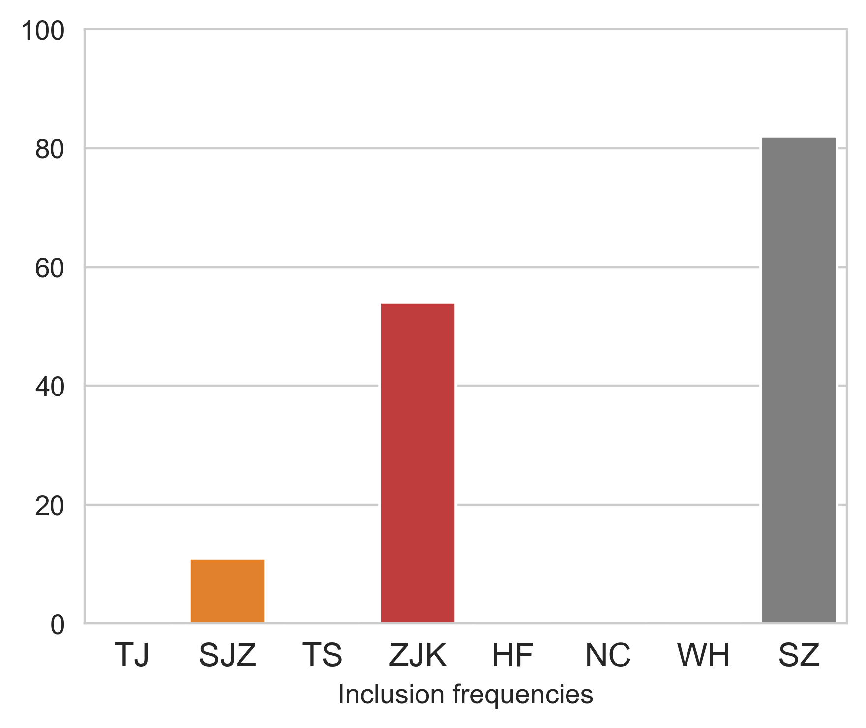
From the perspective of temporal dependence, the air pollution may easily experience dramatic huge changes due to specific events, such as weather changes and human interventions, that is, there exist frequent change points as time goes by, which brings about relatively short time windows for prediction tasks. Besides, if we apply high frequency data to increase the sample size, the excessive dependencies may undermine the effect of our models. Hence we collect the daily datasets as a trade-off between dependencies and sample size. From the perspective of spatial dependence, a notable feature is the geographical similarity, that is, geographically adjacent regions may exhibit similar air quality as a result of the diffusion of air pollution. This feature encourages us to employ information from adjacent regions to increase sample size, in the same spirit of transfer learning. Thus, we collect datasets including Beijing city and eight potential useful cities: Tianjin (TJ), Shijiazhuang (SJZ), Tangshan (TS), Zhangjiakou (ZJK), Hefei (HF), Nanchang (NC), Wuhan (WH) and Shenzhen (SZ). Note that the first four cities are geographically adjacent to Beijing, which might intuitively suffer from similar patterns of air pollution in Beijing.

For each target and source datasets, we collect the daily data from January to February in 2019. In each day $t$, the covariates $\bm{X}_{k,t}$ are matrix-valued data where the rows represent 24 hours and the columns represent the content of six common air pollutants: $\text{PM}_{2.5}$, $\text{PM}_{10}$, $\text{SO}_{2}$, $\text{NO}_{2}$, $\text{O}_{3}$ and CO. The response $y_{k,t}$ is a binary variable, where 1 represents mild pollution while 0 represents relatively good air quality. Clearly, the matrix-valued covariates possess certain column-wise and row-wise correlation, and we add nuclear norm penalty to obtain the low-rank estimation. Specifically, we model the next-day air quality by

$${\mathbb{P}}(y_{k,t+1}|\bm{X}_{k,t})\propto\exp\left\{y_{k,t+1}\langle\bm{\theta}^{*}_{k},\bm{X}_{k,t}\rangle-b(\langle\bm{\theta}^{*}_{k},\bm{X}_{k,t}\rangle)\right\},$$

for the logit link $b^{\prime}(x)=1/(1+e^{-x})$, and use the rolling windows approach with window size 31 to forecast the air pollution of February (28 days). For each day, we set $K=8$, $n_{k}=n_{0}=31$, $p_{1}=24$, $p_{2}=6$, and use respectively the vanilla target estimator, the fine-tuned blind pooling estimator, and the fine-tuned truncated penalized estimator for constructing the next-day prediction.

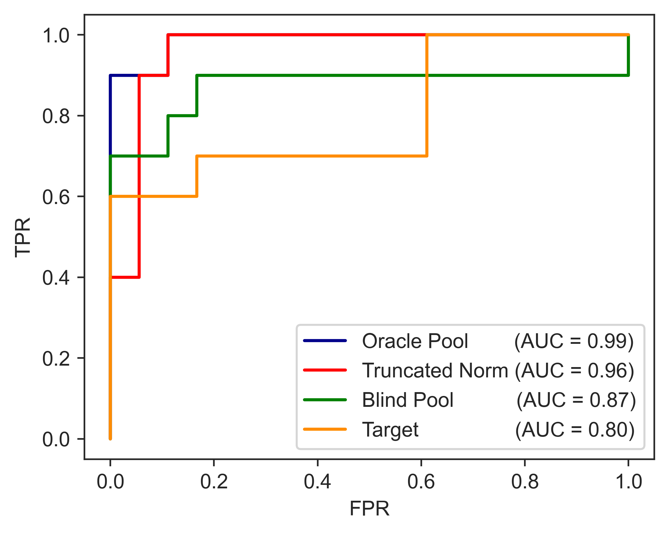
We report the inclusion frequencies of each source dataset in estimating the daily parameters of the Beijing site using the truncated-penalized algorithm on the left panel of Figure 5, which suggests both Zhangjiakou (ZJK), which is geographically adjacent to Beijing, and Shenzhen (SZ) are informative auxiliary datasets for prediction. Here Shenzhen might have been chosen due to similarities in industrial structure, population, and other social factors with Beijing, which implies that selecting auxiliary datasets based on geographical proximity alone may not be sufficient in the air pollution prediction problems. Then, these two sites (ZJK and SZ) are used as the oracle informative source datasets in the backtracking rolling windows, note that such information of useful datasets is not obtained until the end of the month. We could see that the fine-tuned oracle pooling estimator from backtracking reaches the highest area under curve (AUC) score (AUC=0.99) on the right panel of Figure 5, while the fine-tuned truncated-penalized estimator performs comparably (AUC=0.96).

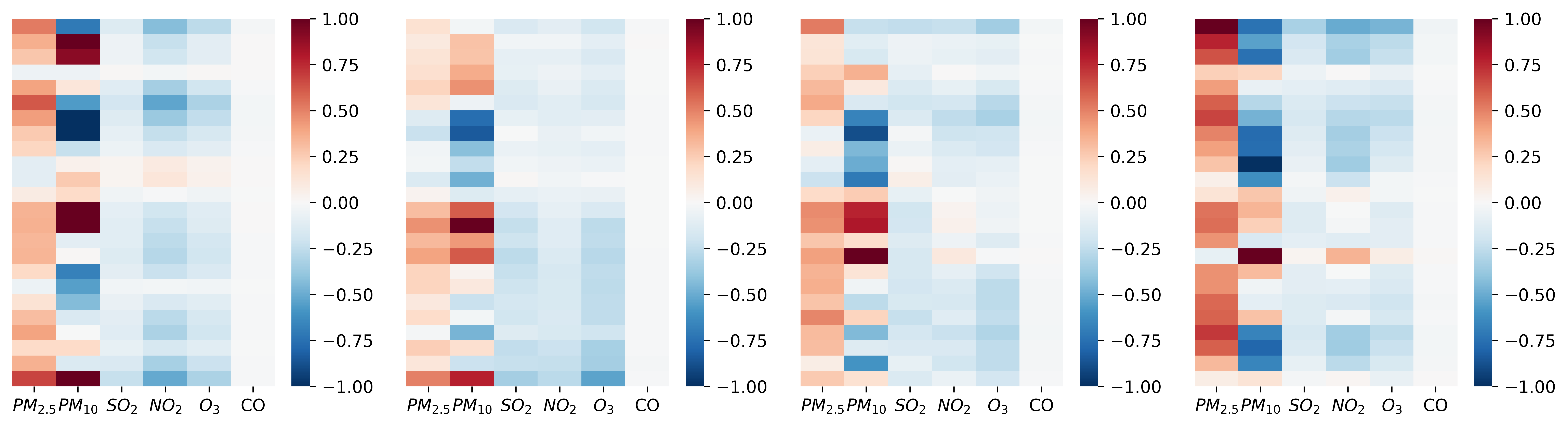
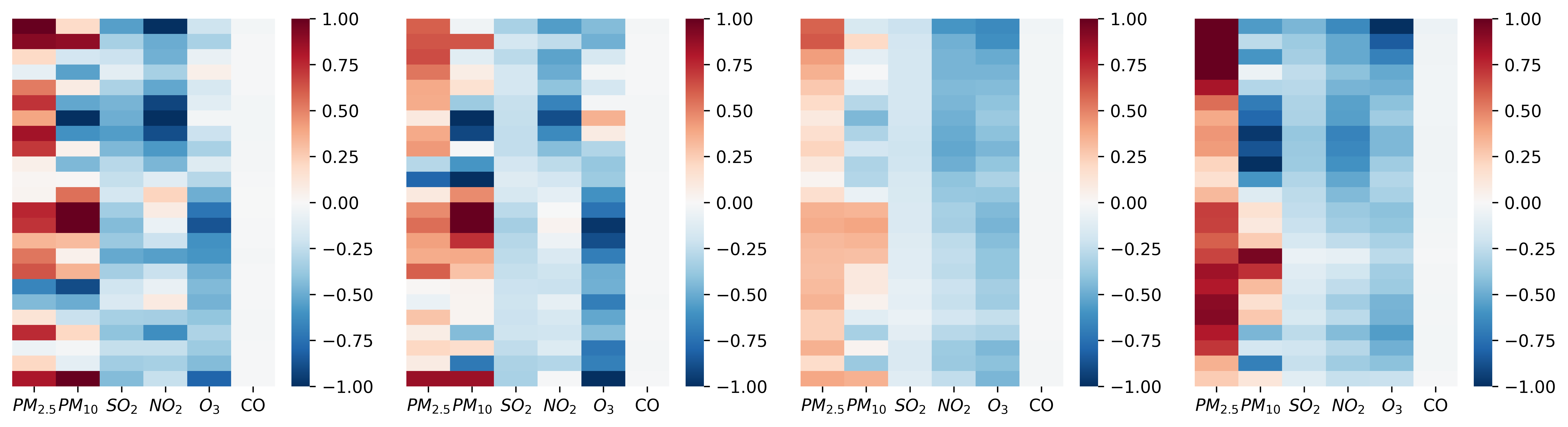
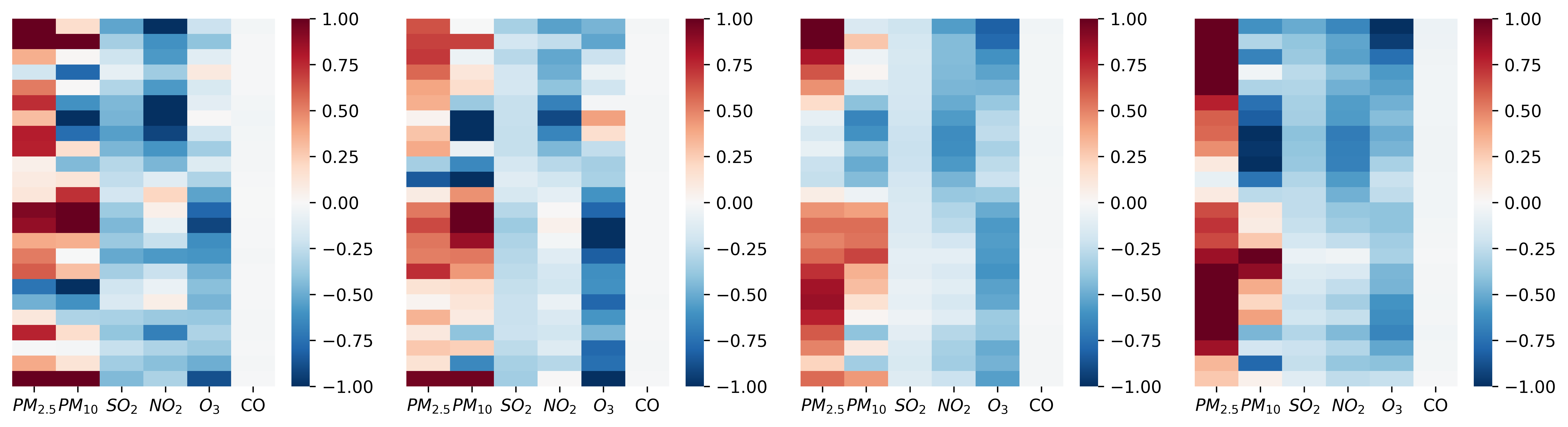
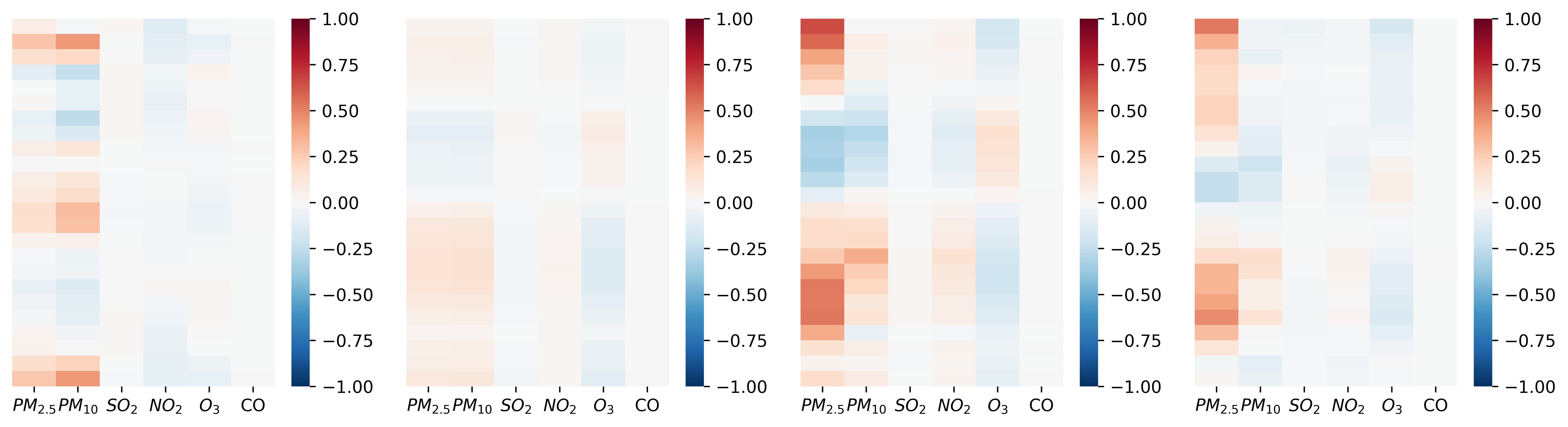
In the end, for better illustration of how transfer learning works in this specific task, we give the heat-maps of the weekly averaged estimators (in the matrix form) in Figure 6. It can be seen from (a) that the air pollution problem in Beijing is strongly related to $\text{PM}_{2.5}$ and $\text{PM}_{10}$, but the effects of other pollutants are somehow underrated or covered. By introducing informative source datasets by the truncated-penalized algorithm, we could see from (b) that additional helpful weights are given on $\text{SO}_{2}$, $\text{NO}_{2}$ and $\text{O}_{3}$. In the end, as shown by (c) and (d), the fine-tuning step re-emphasizes the importance of $\text{PM}_{2.5}$ and $\text{PM}_{10}$ in the case of Beijing, and the fine-tuned truncated-penalized estimator manages to achieve the best performance among the non-backtracking methods.

6 Discussion

In this article, under the high-dimensional M-estimators framework, we highlight the role of fine-tuning hidden underneath the gain of estimating some difference vector with certain low-dimensional structure (debiasing). The theory suggests slightly enlarging the pooling regularization strength if either the contrast’s low-dimensional structure or the homogeneity of Hessian matrices is violated. Specific statistical models are discussed under the framework. When the informative source datasets are unknown, we propose the truncated-penalized algorithm which directly outputs the primal estimator by simultaneously selecting the useful sources. As a potential future work, it is interesting to consider both debiasing and fine-tuning effects at the same time under various knowledge transfer settings.

Acknowledgement

The authors gratefully acknowledge National Science Foundation of China (12171282, 11801316), National Statistical Scientific Research Key Project (2021LZ09), Qilu Young Scholars Program of Shandong University.

References

  • Bai and Silverstein, (2010) Bai, Z. and Silverstein, J. W. (2010). Spectral analysis of large dimensional random matrices, volume 20. Springer.
  • Bai and Silverstein, (1998) Bai, Z.-D. and Silverstein, J. W. (1998). No eigenvalues outside the support of the limiting spectral distribution of large-dimensional sample covariance matrices. The Annals of Probability, 26(1):316–345.
  • Bastani, (2021) Bastani, H. (2021). Predicting with proxies: Transfer learning in high dimension. Management Science, 67(5):2964–2984.
  • Boyd et al., (2011) Boyd, S., Parikh, N., and Chu, E. (2011). Distributed optimization and statistical learning via the alternating direction method of multipliers. Now Publishers Inc.
  • Cai et al., (2010) Cai, J.-F., Candès, E. J., and Shen, Z. (2010). A singular value thresholding algorithm for matrix completion. SIAM Journal on Optimization, 20(4):1956–1982.
  • Cai and Wei, (2021) Cai, T. T. and Wei, H. (2021). Transfer learning for nonparametric classification: Minimax rate and adaptive classifier. The Annals of Statistics, 49(1).
  • Candes and Tao, (2007) Candes, E. and Tao, T. (2007). The dantzig selector: Statistical estimation when p is much larger than n. The Annals of Statistics, 35(6):2313–2351.
  • (8) Fan, J., Gong, W., and Zhu, Z. (2019a). Generalized high-dimensional trace regression via nuclear norm regularization. Journal of Econometrics, 212(1):177–202.
  • (9) Fan, J., Gong, W., and Zhu, Z. (2019b). Generalized high-dimensional trace regression via nuclear norm regularization. Journal of Econometrics, 212(1):177–202.
  • Fan and Li, (2001) Fan, J. and Li, R. (2001). Variable selection via nonconcave penalized likelihood and its oracle properties. Journal of the American statistical Association, 96(456):1348–1360.
  • Fan et al., (2021) Fan, J., Wang, W., and Zhu, Z. (2021). A shrinkage principle for heavy-tailed data: High-dimensional robust low-rank matrix recovery. The Annals of Statistics, 49(3):1239 – 1266.
  • Friedman et al., (2010) Friedman, J., Hastie, T., and Tibshirani, R. (2010). Regularization paths for generalized linear models via coordinate descent. Journal of Statistical Software, 33(1):1–22.
  • Gupta and Nagar, (2018) Gupta, A. K. and Nagar, D. K. (2018). Matrix variate distributions, volume 104. CRC Press.
  • Hamdi and Bayati, (2022) Hamdi, N. and Bayati, M. (2022). On low-rank trace regression under general sampling distribution. The Journal of Machine Learning Research, 23(1):14424–14472.
  • He et al., (2023) He, Y., Kong, X., Trapani, L., and Yu, L. (2023). One-way or two-way factor model for matrix sequences? Journal of Econometrics, in press.
  • He et al., (2022) He, Y., Li, Q., Hu, Q., and Liu, L. (2022). Transfer learning in high-dimensional semiparametric graphical models with application to brain connectivity analysis. Statistics in medicine, 41(21):4112–4129.
  • Lewis, (2010) Lewis, A. D. (2010). A top nine list: Most popular induced matrix norms.
  • (18) Li, S., Cai, T. T., and Li, H. (2022a). Transfer learning for high-dimensional linear regression: Prediction, estimation and minimax optimality. Journal of the Royal Statistical Society Series B: Statistical Methodology, 84(1):149–173.
  • (19) Li, S., Cai, T. T., and Li, H. (2022b). Transfer learning in large-scale gaussian graphical models with false discovery rate control. Journal of the American Statistical Association, pages 1–13.
  • Li et al., (2023) Li, S., Zhang, L., Cai, T. T., and Li, H. (2023). Estimation and inference for high-dimensional generalized linear models with knowledge transfer. Journal of the American Statistical Association, pages 1–12.
  • Liu et al., (2023) Liu, D., Zhao, C., He, Y., Liu, L., Guo, Y., and Zhang, X. (2023). Simultaneous cluster structure learning and estimation of heterogeneous graphs for matrix-variate fmri data. Biometrics.
  • Negahban et al., (2012) Negahban, S. N., Ravikumar, P., Wainwright, M. J., and Yu, B. (2012). A unified framework for high-dimensional analysis of $m$-estimators with decomposable regularizers. Statistical Science, 27(4):538–557.
  • Niu et al., (2020) Niu, S., Liu, Y., Wang, J., and Song, H. (2020). A decade survey of transfer learning (2010–2020). IEEE Transactions on Artificial Intelligence, 1(2):151–166.
  • Pan et al., (2013) Pan, W., Shen, X., and Liu, B. (2013). Cluster analysis: Unsupervised learning via supervised learning with a non-convex penalty. Journal of Machine Learning Research, 14(7):1865–1889.
  • Parikh et al., (2014) Parikh, N., Boyd, S., et al. (2014). Proximal algorithms. Foundations and trends® in Optimization, 1(3):127–239.
  • Qiao et al., (2023) Qiao, S., He, Y., and Zhou, W. (2023). Transfer learning for high-dimensional quantile regression with statistical guarantee. Available upon request.
  • Raskutti et al., (2010) Raskutti, G., Wainwright, M. J., and Yu, B. (2010). Restricted eigenvalue properties for correlated gaussian designs. The Journal of Machine Learning Research, 11:2241–2259.
  • Reeve et al., (2021) Reeve, H. W., Cannings, T. I., and Samworth, R. J. (2021). Adaptive transfer learning. The Annals of Statistics, 49(6):3618–3649.
  • Shen et al., (2012) Shen, X., Pan, W., and Zhu, Y. (2012). Likelihood-based selection and sharp parameter estimation. Journal of the American Statistical Association, 107(497):223–232.
  • Tian and Feng, (2022) Tian, Y. and Feng, Y. (2022). Transfer learning under high-dimensional generalized linear models. Journal of the American Statistical Association, pages 1–14.
  • Tibshirani, (1996) Tibshirani, R. (1996). Regression shrinkage and selection via the lasso. Journal of the Royal Statistical Society: Series B (Methodological), 58(1):267–288.
  • Torrey and Shavlik, (2010) Torrey, L. and Shavlik, J. (2010). Transfer learning. In Handbook of research on machine learning applications and trends: algorithms, methods, and techniques, pages 242–264. IGI global.
  • Vershynin, (2010) Vershynin, R. (2010). Introduction to the non-asymptotic analysis of random matrices. arXiv preprint arXiv:1011.3027.
  • Wu et al., (2016) Wu, C., Kwon, S., Shen, X., and Pan, W. (2016). A new algorithm and theory for penalized regression-based clustering. The Journal of Machine Learning Research, 17(1):6479–6503.
  • Yin et al., (1988) Yin, Y.-Q., Bai, Z.-D., and Krishnaiah, P. R. (1988). On the limit of the largest eigenvalue of the large dimensional sample covariance matrix. Probability theory and related fields, 78:509–521.
  • Zhou and Li, (2014) Zhou, H. and Li, L. (2014). Regularized matrix regression. Journal of the Royal Statistical Society. Series B, Statistical Methodology, 76(2):463.
  • Zhuang et al., (2020) Zhuang, F., Qi, Z., Duan, K., Xi, D., Zhu, Y., Zhu, H., Xiong, H., and He, Q. (2020). A comprehensive survey on transfer learning. Proceedings of the IEEE, 109(1):43–76.

Appendix

Appendix A Useful Results of Negahban et al., (2012)

Useful results of Negahban et al., (2012) are stated here for convenience. First, suppose $L$ is a convex and differentiable function, consider the following optimization problem:

$$\widehat{\bm{\theta}}=\mathop{\text{\rm arg\,min}}_{\bm{\theta}\in{\mathbb{R}}^{p}}\left\{L(\bm{\theta})+\lambda{\mathcal{R}}(\bm{\theta})\right\}.$$ (13)

For given $\bm{\theta}^{*}$, if we have the regularization parameter satisfy $\lambda\geq 2{\mathcal{R}}^{*}\left(\nabla L(\bm{\theta}^{*})\right)$, where ${\mathcal{R}}^{*}(\bm{v})=\sup_{{\mathcal{R}}(\bm{u})\leq 1}\langle\bm{u},\bm{v}\rangle$ is the dual norm of ${\mathcal{R}}$, then for any subspace pair $({\mathcal{M}},\overline{{\mathcal{M}}}^{\perp})$ over which ${\mathcal{R}}$ is decomposable, the error $\widehat{\bm{\Delta}}=\widehat{\bm{\theta}}-\bm{\theta}^{*}$ belongs to the cone-like set

$${\mathbb{C}}\left(\mathcal{M},\overline{\mathcal{M}}^{\perp};\bm{\theta}^{*}\right):=\left\{\bm{\Delta}\in\mathbb{R}^{p}\mid\mathcal{R}\left(\bm{\Delta}_{\overline{\mathcal{M}}^{\perp}}\right)\leq 3\mathcal{R}\left(\bm{\Delta}_{\overline{\mathcal{M}}}\right)+4{\mathcal{R}}(\bm{\theta}^{*}_{{\mathcal{M}}^{\perp}})\right\}.$$

Then, we need to impose restricted strong convexity (RSC) on this set, define

$$\delta L(\bm{\Delta};\bm{\theta}^{*})=L(\bm{\theta}^{*}+\bm{\Delta})-L(\bm{\theta}^{*})-\left\langle\nabla L(\bm{\theta}^{*}),\bm{\Delta}\right\rangle,$$

we say the loss function $L$ satisfies a restricted strong convexity condition on $\bm{\theta}^{*}$ with curvature $\kappa_{L}>0$ and tolerance term $\tau_{L}\geq 0$ if

$$\delta L(\bm{\Delta};\bm{\theta}^{*})\geq\kappa_{L}\|\bm{\Delta}\|^{2}-\tau_{L},\quad\text{for all }\bm{\Delta}\in{\mathbb{C}}\left(\mathcal{M},\overline{\mathcal{M}}^{\perp};\bm{\theta}^{*}\right).$$

With the arguments above in hand, namely given sufficiently large regularization $\lambda$ and RSC of loss function $L$, we are able to bound the error term of problem (13) by

$$\|\widehat{\bm{\theta}}-\bm{\theta}^{*}\|^{2}\leq 9\frac{\lambda^{2}}{\kappa_{L}^{2}}\Psi^{2}(\overline{{\mathcal{M}}})+\frac{\lambda}{\kappa_{L}}\left\{2\tau_{L}+4{\mathcal{R}}(\bm{\theta}^{*}_{{\mathcal{M}}^{\perp}})\right\},$$

where $\Psi({\mathcal{M}})=\sup_{\bm{u}\in{\mathcal{M}}\backslash\{0\}}{\mathcal{R}}(\bm{u})/\|\bm{u}\|$ is called the subspace compatibility constant measuring the degree of compatibility between ${\mathcal{R}}(\cdot)$ and $\|\cdot\|$.

Appendix B Proof of main results

Here we present the proof of main results in the article.

B.1 Proof of Lemma 1

The arguments follows directly from Negahban et al., (2012). First, given $\lambda_{\mathcal{P}}\geq 2{\mathcal{R}}^{*}\left(\nabla\bm{L}_{\mathcal{P}}(\bm{\theta}^{*}_{0})\right)$ and $\bm{\theta}^{*}_{0}\in\mathcal{M}$, we have $\widehat{\bm{\theta}}_{\mathcal{P}}-\bm{\theta}^{*}_{0}$ lies in the cone:

$$\mathbb{C}\left(\mathcal{M},\overline{\mathcal{M}}^{\perp};\bm{\theta}^{*}_{0}\right):=\left\{\bm{\Delta}\in{\mathbb{R}}^{p}\mid\mathcal{R}\left(\bm{\Delta}_{\overline{\mathcal{M}}^{\perp}}\right)\leq 3\mathcal{R}\left(\bm{\Delta}_{\overline{\mathcal{M}}}\right)\right\}.$$

Then, by the RSC condition on $\mathbb{C}\left(\mathcal{M},\overline{\mathcal{M}}^{\perp};\bm{\theta}^{*}_{0}\right)$, for $\bm{\delta}^{\widehat{*}}=\bm{\theta}^{*}_{0}-\widehat{\bm{\theta}}_{\mathcal{P}}$, we have by Theorem 1 in Negahban et al., (2012) that

$$\|\bm{\delta}^{\widehat{*}}\|^{2}=\|\widehat{\bm{\theta}}_{\mathcal{P}}-\bm{\theta}^{*}_{0}\|^{2}\leq 9\frac{\lambda_{\mathcal{P}}^{2}}{\kappa_{\mathcal{P}}^{2}}\Psi^{2}(\overline{\mathcal{M}})+2\frac{\lambda_{\mathcal{P}}}{\kappa_{\mathcal{P}}}\tau_{\mathcal{P}}.$$ (14)

Recall that $\bm{\delta}^{\widehat{*}}\in\mathbb{C}\left(\mathcal{M},\overline{\mathcal{M}}^{\perp};\bm{\theta}^{*}_{0}\right)$, we eventually have

$\displaystyle\mathcal{R}(\bm{\delta}^{\widehat{*}})$ $\displaystyle\leq\mathcal{R}\left(\bm{\delta}^{\widehat{*}}_{\overline{\mathcal{M}}}\right)+\mathcal{R}\left(\bm{\delta}^{\widehat{*}}_{\overline{\mathcal{M}}^{\perp}}\right)\leq 4\mathcal{R}\left(\bm{\delta}^{\widehat{*}}_{\overline{\mathcal{M}}}\right)$ (15)
$\displaystyle\leq 4\Psi(\overline{\mathcal{M}})\|\bm{\delta}^{\widehat{*}}\|.$

Since $\tau_{\mathcal{P}}\lesssim\lambda_{\mathcal{P}}\Psi^{2}(\overline{\mathcal{M}})/\kappa_{\mathcal{P}}$ by assumption, combine (14) and (15), we eventually have

$$\|\bm{\delta}^{\widehat{*}}\|^{2}\lesssim\frac{\lambda^{2}_{\mathcal{P}}}{\kappa^{2}_{\mathcal{P}}}\Psi^{2}(\overline{\mathcal{M}}),\quad\mathcal{R}(\bm{\delta}^{\widehat{*}})\lesssim\frac{\lambda_{\mathcal{P}}}{\kappa_{\mathcal{P}}}\Psi^{2}(\overline{\mathcal{M}}).$$

B.2 Proof of Theorem 1

Under the conditions in Lemma 1, for $\bm{\delta}^{\widehat{*}}=\bm{\theta}^{*}_{0}-\widehat{\bm{\theta}}_{\mathcal{P}}$, we have ${\mathcal{R}}(\bm{\delta}^{\widehat{*}})\leq l_{\mathcal{P}}$ from the pooling step for some $l_{\mathcal{P}}\asymp\lambda_{\mathcal{P}}\Psi^{2}(\overline{\mathcal{M}})/\kappa_{\mathcal{P}}$. Then we introduce the following results concerning the second step in both constrained and Lagrangian forms.

Lemma 2 (Constrained Fine-tuning).

Assume that $\mathcal{R}(\bm{\delta}^{\widehat{*}})\leq l_{\mathcal{P}}$, suppose $\bm{L}_{0}$ is convex, differentiable and satisfies the RSC condition such that

$$\delta\bm{L}_{0}(\bm{\Delta};\bm{\theta}^{*}_{0})\geq\kappa_{d}\|\bm{\Delta}\|^{2}-\tau_{d},\quad\text{for all }\mathcal{R}(\bm{\Delta})\leq 2l_{\mathcal{P}},$$ (16)

we have the optimal solution to the constrained fine-tuning problem (6) with respect to $l_{\mathcal{P}}$ satisfies

$$\|\widehat{\bm{\delta}}-\bm{\delta}^{\widehat{*}}\|^{2}\lesssim\frac{R^{*}(\nabla\bm{L}_{0}(\bm{\theta}^{*}_{0}))l_{\mathcal{P}}}{\kappa_{d}}+\frac{\tau_{d}}{\kappa_{d}}.$$
Lemma 3 (Lagrangian Fine-tuning).

Assume that $\mathcal{R}(\bm{\delta}^{\widehat{*}})\leq l_{\mathcal{P}}$, suppose $\bm{L}_{0}$ is convex, differentiable and satisfies the RSC condition such that

$$\delta\bm{L}_{0}(\bm{\Delta};\bm{\theta}^{*}_{0})\geq\kappa_{d}\|\bm{\Delta}\|^{2}-\tau_{d},\quad\text{for all }\mathcal{R}(\bm{\Delta})\leq 4l_{\mathcal{P}},$$ (17)

then the optimal solution to the Lagrangian fine-tuning problem (7) with respect to $\lambda_{d}\geq 2R^{*}(\nabla\bm{L}_{0}(\bm{\theta}^{*}_{0}))$ satisfies

$$\|\widehat{\bm{\delta}}-\bm{\delta}^{\widehat{*}}\|^{2}\lesssim\frac{\lambda_{d}l_{\mathcal{P}}}{\kappa_{d}}+\frac{\tau_{d}}{\kappa_{d}}.$$

In the end, since $\tau_{d}\lesssim\lambda_{d}l_{\mathcal{P}}$ by assumption, the proof is claimed. Then, we present the proofs of Lemma 2 and Lemma 3.

B.2.1 Proof of Lemma 2

Here we define $\bm{L}_{d}(\bm{\delta})=\bm{L}_{0}(\widehat{\bm{\theta}}_{\mathcal{P}}+\bm{\delta})$, note that $\bm{L}_{d}$ is merely translation of $\bm{L}_{0}$ to the new center $\widehat{\bm{\theta}}_{\mathcal{P}}$, so we have $\delta\bm{L}_{d}(\bm{\Delta};\bm{\delta}^{\widehat{*}})=\delta\bm{L}_{0}(\bm{\Delta};\bm{\theta}^{*}_{0})$ and $\mathcal{R}^{*}(\nabla\bm{L}_{d}(\bm{\delta}^{\widehat{*}}))=\mathcal{R}^{*}(\nabla\bm{L}_{0}(\bm{\theta}^{*}_{0}))$. For $\widehat{\bm{\Delta}}=\widehat{\bm{\delta}}-\bm{\delta}^{\widehat{*}}$, since $\mathcal{R}(\bm{\delta}^{\widehat{*}}+\widehat{\bm{\Delta}})\leq l_{\mathcal{P}}$, we have $\mathcal{R}(\widehat{\bm{\Delta}})\leq 2l_{\mathcal{P}}$ and by the RSC condition (16),

$\displaystyle\bm{L}_{d}(\bm{\delta}^{\widehat{*}}+\widehat{\bm{\Delta}})$ $\displaystyle\geq\bm{L}_{d}(\bm{\delta}^{\widehat{*}})+\langle\nabla\bm{L}_{d}(\bm{\delta}^{\widehat{*}}),\widehat{\bm{\Delta}}\rangle+\kappa_{d}\|\widehat{\bm{\Delta}}\|^{2}-\tau_{d}$
$\displaystyle\geq\bm{L}_{d}(\bm{\delta}^{\widehat{*}})+\left[\kappa_{d}\|\widehat{\bm{\Delta}}\|^{2}-\mathcal{R}^{*}(\nabla\bm{L}_{d}(\bm{\delta}^{\widehat{*}}))\mathcal{R}(\widehat{\bm{\Delta}})-\tau_{d}\right]$
$\displaystyle\geq\bm{L}_{d}(\bm{\delta}^{\widehat{*}})+\left[\kappa_{d}\|\widehat{\bm{\Delta}}\|^{2}-2\mathcal{R}^{*}(\nabla\bm{L}_{d}(\bm{\delta}^{\widehat{*}}))l_{\mathcal{P}}-\tau_{d}\right].$

Note that we need $\bm{L}_{d}(\bm{\delta}^{\widehat{*}}+\widehat{\bm{\Delta}})\leq\bm{L}_{d}(\bm{\delta}^{\widehat{*}})$, it requires $\kappa_{d}\|\widehat{\bm{\Delta}}\|^{2}\leq 2\mathcal{R}^{*}(\nabla\bm{L}_{d}(\bm{\delta}^{\widehat{*}}))l_{\mathcal{P}}+\tau_{d}$, the rest is straightforward.

B.2.2 Proof of Lemma 3

Similarly, define $\bm{L}_{d}(\bm{\delta})=\bm{L}_{0}(\widehat{\bm{\theta}}_{\mathcal{P}}+\bm{\delta})$, by convexity of $\bm{L}_{d}$ and triangular inequality we have

$$\bm{L}_{d}(\bm{\delta}^{\widehat{*}}+\bm{\Delta})+\lambda_{d}\mathcal{R}(\bm{\delta}^{\widehat{*}}+\bm{\Delta})\geq\bm{L}_{d}(\bm{\delta}^{\widehat{*}})+\langle\nabla\bm{L}_{d}(\bm{\delta}^{\widehat{*}}),\bm{\Delta}\rangle+\lambda_{d}\mathcal{R}(\bm{\Delta})-\lambda_{d}\mathcal{R}(\bm{\delta}^{\widehat{*}}).$$

Note that for $\widehat{\bm{\Delta}}=\widehat{\bm{\delta}}-\bm{\delta}^{\widehat{*}}$ we need $\bm{L}_{d}(\bm{\delta}^{\widehat{*}}+\widehat{\bm{\Delta}})+\lambda_{d}\mathcal{R}(\bm{\delta}^{\widehat{*}}+\widehat{\bm{\Delta}})\leq\bm{L}_{d}(\bm{\delta}^{\widehat{*}})+\lambda_{d}\mathcal{R}(\bm{\delta}^{\widehat{*}})$ and $\lambda_{d}\geq 2\mathcal{R}^{*}\left(\nabla\bm{L}_{d}(\bm{\delta}^{\widehat{*}})\right)$, which yields

$\displaystyle 2\lambda_{d}\mathcal{R}(\bm{\delta}^{\widehat{*}})$ $\displaystyle\geq\lambda_{d}\mathcal{R}(\widehat{\bm{\Delta}})+\langle\nabla\bm{L}_{d}(\bm{\delta}^{\widehat{*}}),\widehat{\bm{\Delta}}\rangle$
$\displaystyle\geq\lambda_{d}\mathcal{R}(\widehat{\bm{\Delta}})-\mathcal{R}^{*}\left(\nabla\bm{L}_{d}(\bm{\delta}^{\widehat{*}})\right)\mathcal{R}(\widehat{\bm{\Delta}})$
$\displaystyle\geq\lambda_{d}\mathcal{R}(\widehat{\bm{\Delta}})/2,$

which directly gives $\mathcal{R}(\widehat{\bm{\Delta}})\leq 4l_{\mathcal{P}}$. Then by the RSC condition (17) we have

$\displaystyle\bm{L}_{d}(\bm{\delta}^{\widehat{*}}+\widehat{\bm{\Delta}})$ $\displaystyle\geq\bm{L}_{d}(\bm{\delta}^{\widehat{*}})+\langle\nabla\bm{L}_{d}(\bm{\delta}^{\widehat{*}}),\widehat{\bm{\Delta}}\rangle+\kappa_{d}\|\widehat{\bm{\Delta}}\|^{2}-\tau_{d}$
$\displaystyle\geq\bm{L}_{d}(\bm{\delta}^{\widehat{*}})+\left[\kappa_{d}\|\widehat{\bm{\Delta}}\|^{2}-\mathcal{R}^{*}(\nabla\bm{L}_{d}(\bm{\delta}^{\widehat{*}}))\mathcal{R}(\widehat{\bm{\Delta}})-\tau_{d}\right]$
$\displaystyle\geq\bm{L}_{d}(\bm{\delta}^{\widehat{*}})+\left[\kappa_{d}\|\widehat{\bm{\Delta}}\|^{2}-2\mathcal{R}^{*}(\nabla\bm{L}_{d}(\bm{\delta}^{\widehat{*}}))l_{\mathcal{P}}-\tau_{d}\right].$

In the end, since $\bm{L}_{d}(\bm{\delta}^{\widehat{*}})+\lambda_{d}\mathcal{R}(\bm{\delta}^{\widehat{*}})\geq\bm{L}_{d}(\bm{\delta}^{\widehat{*}}+\widehat{\bm{\Delta}})+\lambda_{d}\mathcal{R}(\bm{\delta}^{\widehat{*}}+\widehat{\bm{\Delta}})\geq\bm{L}_{d}(\bm{\delta}^{\widehat{*}}+\widehat{\bm{\Delta}})$, we have $\kappa_{d}\|\widehat{\bm{\Delta}}\|^{2}\leq 2\mathcal{R}^{*}(\nabla\bm{L}_{d}(\bm{\delta}^{\widehat{*}}))l_{\mathcal{P}}+\lambda_{d}\mathcal{R}(\bm{\delta}^{\widehat{*}})+\tau_{d}\lesssim\lambda_{d}l_{\mathcal{P}}+\tau_{d}$, the rest is straightforward.

B.3 Proof of Theorem 2

First, for the restricted strong convexity (RSC) conditions, we take the following result from Raskutti et al., (2010), such that there are positive constants $\left(\kappa_{k,1},\kappa_{k,2}\right)$, depending only on $\bm{\Sigma}_{k}$, for $\widehat{\bm{\Sigma}}_{k}=\mathbf{\mathcal{X}}_{k}^{\top}\mathbf{\mathcal{X}}_{k}/n_{k}$,

$$\left\langle\bm{\Delta},\widehat{\bm{\Sigma}}_{k}\bm{\Delta}\right\rangle\geq\kappa_{k,1}\|\bm{\Delta}\|^{2}-\kappa_{k,2}\frac{\log p}{n_{k}}\|\bm{\Delta}\|_{1}^{2},\quad\text{for all }\bm{\Delta}\in{\mathbb{R}}^{p}.$$ (18)

with probability greater than $1-c_{k,1}\exp\left(-c_{k,2}n_{k}\right)$. We then focus on the Hessian matrix of $\bm{L}_{\mathcal{P}}$, which is $\sum_{k\in\mathcal{P}}n_{k}\widehat{\bm{\Sigma}}_{k}/n_{\mathcal{P}}$, and the Hessian matrix of $\bm{L}_{0}$, which is $\widehat{\bm{\Sigma}}_{0}$.

Lemma 4 (RSC Conditions).

Under the settings of section 3.2.1, let $\bm{\Delta}_{s}$ (or $\bm{\Delta}_{s^{c}}$) be the projection of $\bm{\Delta}$ onto the $s$-sparse support (or its complement), there exist positive constants $(\kappa_{\mathcal{P},1},\kappa_{\mathcal{P},2})$ such that

$$\frac{1}{n_{\mathcal{P}}}\left\langle\bm{\Delta},\sum_{k\in\mathcal{P}}n_{k}\widehat{\bm{\Sigma}}_{k}\bm{\Delta}\right\rangle\geq\left[\kappa_{\mathcal{P},1}-\kappa_{\mathcal{P},2}\frac{\log p}{n_{\mathcal{P}}}\right]\|\bm{\Delta}\|^{2},\quad\text{for all }\|\bm{\Delta}_{s^{c}}\|_{1}\leq 3\|\bm{\Delta}_{s}\|_{1},$$ (19)

with probability greater than $1-\sum_{k\in\mathcal{P}}c_{k,1}\exp\left(-c_{k,2}n_{k}\right)$. In addition, within this event, we have

$$\left\langle\bm{\Delta},\widehat{\bm{\Sigma}}_{0}\bm{\Delta}\right\rangle\geq\kappa_{0,1}\|\bm{\Delta}\|^{2}-\kappa_{0,2}\frac{\log p}{n_{0}}(c_{0}l_{\mathcal{P}})^{2},\quad\text{for all }\|\bm{\Delta}\|_{1}\leq c_{0}l_{\mathcal{P}}.$$ (20)

Then we give the following result concerning the rate of $\mathcal{R}^{*}\left(\nabla\bm{L}_{\mathcal{P}}(\bm{\theta}^{*}_{0})\right)$ and $\mathcal{R}^{*}(\nabla\bm{L}_{0}(\bm{\theta}^{*}_{0}))$.

Lemma 5 (Convergence Rates).

Under the settings of section 3.2.1, we have as $\min_{k\in\mathcal{P}}n_{k}\rightarrow\infty$, $p\rightarrow\infty$ and $h\rightarrow 0$,

$$\mathcal{R}^{*}\left(\nabla\bm{L}_{\mathcal{P}}(\bm{\theta}^{*}_{0})\right)=\underbrace{O_{p}(\sqrt{\frac{\log p}{n_{\mathcal{P}}}}+h)}_{v_{\mathcal{P}}+b_{\mathcal{P}}},\quad\mathcal{R}^{*}(\nabla\bm{L}_{0}(\bm{\theta}^{*}_{0}))=\underbrace{O_{p}(\sqrt{\frac{\log p}{n_{0}}})}_{v_{0}}.$$ (21)

With the help of Lemma 4 and Lemma 5, by assuming $\log p\lesssim n_{0}$ and $(\log p/n_{\mathcal{P}})^{1/2}+h\rightarrow 0$, we have $\tau_{d}\asymp(\lambda_{d}l_{\mathcal{P}})^{2}\ll\lambda_{d}l_{\mathcal{P}}$, and Theorem 2 holds according to Theorem 1. Then we give the proof of Lemma 4 and Lemma 5.

B.3.1 Proof of Lemma 4

These are the straightforward consequences of (18). For $\|\bm{\Delta}_{s^{c}}\|_{1}\leq 3\|\bm{\Delta}_{s}\|_{1}$, we have $\|\bm{\Delta}\|_{1}=\|\bm{\Delta}_{s}\|_{1}+\|\bm{\Delta}_{s^{c}}\|_{1}\leq 4\|\bm{\Delta}_{s}\|_{1}\leq 4\sqrt{s}\|\bm{\Delta}\|$, then we have (19) holds with $\kappa_{\mathcal{P},1}=\sum_{k\in\mathcal{P}}n_{k}\kappa_{k,1}/n_{\mathcal{P}}$ and $\kappa_{\mathcal{P},2}=\sum_{k\in\mathcal{P}}16s\kappa_{k,2}$ by the union bound of probability. On the other hand, (20) holds by plugging in $\|\bm{\Delta}\|_{1}\leq c_{0}l_{\mathcal{P}}$ to (18).

B.3.2 Proof of Lemma 5

Controlling $\mathcal{R}^{*}(\nabla\bm{L}_{0}(\bm{\theta}^{*}_{0}))\asymp\|\mathbf{\mathcal{X}}_{0}^{\top}\bm{\epsilon}_{0}\|_{\infty}/n_{0}$ is straightforward by noticing that the maximum of a $p$-dimensional vector with sub-Gaussian elements, with variance proxies of order $n_{0}$, is controlled by $(n_{0}\log p)^{1/2}$ using standard union bound arguments. As for $\mathcal{R}^{*}\left(\nabla\bm{L}_{\mathcal{P}}(\bm{\theta}^{*}_{0})\right)$, for $h$ sufficiently small, it suffices to bound $v_{\mathcal{P}}=\mathcal{R}^{*}\left(\sum_{k\in\mathcal{P}}n_{k}\nabla\bm{L}_{k}(\bm{\theta}^{*}_{k})\right)/n_{\mathcal{P}}$ and $b_{\mathcal{P}}=\sum_{k\in\mathcal{P}}n_{k}\mathcal{R}^{*}\left(\nabla^{2}\bm{L}_{k}(\bm{\theta}^{*}_{k})\bm{\delta}^{*}_{k}\right)/n_{\mathcal{P}}$. First, $v_{\mathcal{P}}\asymp\|\sum_{k\in\mathcal{P}}\mathbf{\mathcal{X}}_{k}^{\top}\bm{\epsilon}_{k}\|_{\infty}/n_{\mathcal{P}}=O_{p}(\sqrt{\log p/n_{\mathcal{P}}})$ by noticing that each element of $\sum_{k\in\mathcal{P}}\mathbf{\mathcal{X}}_{k}^{\top}\bm{\epsilon}_{k}$ is the sum of $n_{\mathcal{P}}$ independent centered random variables and is of order $n_{\mathcal{P}}^{1/2}$, then we have the result by similar union bound arguments. In the end, for $b_{\mathcal{P}}=\sum_{k\in\mathcal{P}}n_{k}\mathcal{R}^{*}\left(\nabla^{2}\bm{L}_{k}(\bm{\theta}^{*}_{k})\bm{\delta}^{*}_{k}\right)/n_{\mathcal{P}}$, we proceed by controlling each term $\|\mathbf{\mathcal{X}}_{k}^{\top}\mathbf{\mathcal{X}}_{k}\bm{\delta}^{*}_{k}\|_{\infty}/n_{\mathcal{P}}$. Recall that for $m\times n$ matrix $\bm{A}=(a_{ij})$ and its transpose $\bm{A}^{\top}=\left((\bm{A}^{\top})_{1},\cdots,(\bm{A}^{\top})_{m}\right)$, we have

$$\|\bm{A}\|_{1\rightarrow\infty}=\sup_{\|v\|_{1}\leq 1}\|\bm{A}v\|_{\infty}=\max_{(i,j)\in\{1,\ldots,m\}\times\{1,\ldots,n\}}\left|a_{ij}\right|,$$
$$\|\bm{A}\|_{2\rightarrow\infty}=\sup_{\|\bm{v}\|_{2}\leq 1}\|\bm{A}\bm{v}\|_{\infty}=\max_{i=1,\ldots,m}\left\|(\bm{A}^{\top})_{i}\right\|_{2},$$

so that $\|\mathbf{\mathcal{X}}_{k}^{\top}\mathbf{\mathcal{X}}_{k}\mathbf{\mathcal{X}}_{k}\bm{\delta}^{*}_{k}\|_{\infty}\leq\|\mathbf{\mathcal{X}}_{k}^{\top}\mathbf{\mathcal{X}}_{k}\|_{1\rightarrow\infty}\|\bm{\delta}^{*}_{k}\|_{1}$, or $\|\mathbf{\mathcal{X}}_{k}^{\top}\mathbf{\mathcal{X}}_{k}\bm{\delta}^{*}_{k}\|_{\infty}\leq\|\mathbf{\mathcal{X}}_{k}^{\top}\mathbf{\mathcal{X}}_{k}\|_{2\rightarrow\infty}\|\bm{\delta}^{*}_{k}\|_{2}$. Note that by Cauchy-Schwarz inequality, the maximum of $|(\mathbf{\mathcal{X}}_{k}^{\top}\mathbf{\mathcal{X}}_{k})_{ij}|$ is obtained on diagonal, where $(\mathbf{\mathcal{X}}_{k}^{\top}\mathbf{\mathcal{X}}_{k})_{ii}=n_{k}(\bm{\Sigma}_{k})_{i,i}+O_{p}(n_{k}^{1/2})$, so that $\|\mathbf{\mathcal{X}}_{k}^{\top}\mathbf{\mathcal{X}}_{k}\bm{\delta}^{*}_{k}\|_{\infty}\lesssim n_{k}h$ in probability as $n_{k}\rightarrow\infty$ if $\|\bm{\delta}^{*}_{k}\|_{1}\leq h$. On the other hand, $\|\mathbf{\mathcal{X}}_{k}^{\top}\mathbf{\mathcal{X}}_{k}\|_{2\rightarrow\infty}\leq\lambda_{\max}(\mathbf{\mathcal{X}}_{k}^{\top}\mathbf{\mathcal{X}}_{k})\leq M_{3}n_{k}$ almost surely if $p/n_{k}\rightarrow c_{k}$ as $n_{k}$, $p\rightarrow\infty$ according to Yin et al., (1988); Bai and Silverstein, (1998, 2010) for $\|\bm{\delta}^{*}_{k}\|_{2}\leq h$. The proof is complete.

B.4 Proof of Theorem 3

We first verify the RSC conditions under the settings of section 3.2.2. Since $\|{\mathop{\text{\rm vec}}}(\bm{X}_{k,i})\|_{\Psi_{2}}\leq M_{1}$ and $\lambda_{\min}\left[\bm{H}_{k}(\bm{\theta}^{*}_{k})\right]\geq\kappa_{k}$ for $k\in\mathcal{P}$, according to (6.11) of Fan et al., 2019a , with probability $1-\exp(-c_{k}d)$,

$$\left\langle{\mathop{\text{\rm vec}}}(\bm{\Delta}),\widehat{\bm{H}}_{k}(\bm{\theta}^{*}_{k}){\mathop{\text{\rm vec}}}(\bm{\Delta})\right\rangle\geq\kappa_{k,1}\|\bm{\Delta}\|_{F}^{2}-\kappa_{k,2}\sqrt{\frac{d}{n_{k}}}\|\bm{\Delta}\|_{N}^{2},\quad\text{for all }\bm{\Delta}\in{\mathbb{R}}^{d\times d}.$$ (22)

As for the rate of convergence, given $\|{\mathop{\text{\rm vec}}}(\bm{X}_{k,i})\|_{\Psi_{2}}\leq M_{1}$ and $|b^{\prime\prime}(\eta_{k,i})|\leq M_{2}$ almost surely, according to Lemma 1 of Fan et al., 2019a , for $d\lesssim n_{k}$, as $d\rightarrow\infty$,

$$\left\|\frac{1}{n_{k}}\sum_{i\leq n_{k}}\left[b^{\prime}\left(\langle\bm{\theta}^{*}_{k},\bm{X}_{k,i}\rangle\right)-y_{k,i}\right]\bm{X}_{k,i}\right\|_{\text{op}}=O_{p}(\sqrt{\frac{d}{n_{k}}}).$$ (23)

Then, we establish Lemma 6 and Lemma 7 based on (22) and (23).

Lemma 6 (RSC Conditions).

Under the settings of section 3.2.2, for $\bm{\delta}^{*}_{k}=\bm{\theta}^{*}_{0}-\bm{\theta}^{*}_{k}$, let $\bm{\Delta}_{\overline{\mathcal{M}}}$ (or $\bm{\Delta}_{\overline{\mathcal{M}}^{\perp}}$) be the projection of $\bm{\Delta}$ onto $\overline{\mathcal{M}}$ (or $\overline{\mathcal{M}}^{\perp}$). Denote $\widehat{\bm{H}}_{\mathcal{P}}=\nabla^{2}\bm{L}_{\mathcal{P}}=\sum_{k\in\mathcal{P}}n_{k}\widehat{\bm{H}}_{k}/n_{\mathcal{P}}$. For some positive constant $\kappa_{\mathcal{P}}$, as $n_{\mathcal{P}}\rightarrow\infty$, $d\rightarrow\infty$ with $d/n_{\mathcal{P}}\rightarrow 0$ and $h\rightarrow 0$, we have

$$\left\langle{\mathop{\text{\rm vec}}}(\bm{\Delta}),\widehat{\bm{H}}_{\mathcal{P}}(\bm{\theta}^{*}_{0}){\mathop{\text{\rm vec}}}(\bm{\Delta})\right\rangle\geq\kappa_{\mathcal{P}}\|\bm{\Delta}\|_{F}^{2},\quad\text{for all }\|\bm{\Delta}_{\overline{\mathcal{M}}^{\perp}}\|_{N}\leq 3\|\bm{\Delta}_{\overline{\mathcal{M}}}\|_{N},$$ (24)

with probability tending to 1. In addition, within this event, we have

$$\left\langle{\mathop{\text{\rm vec}}}(\bm{\Delta}),\widehat{\bm{H}}_{0}(\bm{\theta}^{*}_{0}){\mathop{\text{\rm vec}}}(\bm{\Delta})\right\rangle\geq\kappa_{0,1}\|\bm{\Delta}\|_{F}^{2}-\kappa_{0,2}\sqrt{\frac{d}{n_{0}}}(c_{0}l_{\mathcal{P}})^{2},\quad\text{for all }\|\bm{\Delta}\|_{N}\leq c_{0}l_{\mathcal{P}}.$$ (25)
Lemma 7 (Convergence Rates).

Under the settings of section 3.2.2, assume that $d\lesssim n_{0}$, we have as $d\rightarrow\infty$ and $h\rightarrow 0$,

$$\mathcal{R}^{*}\left(\nabla\bm{L}_{\mathcal{P}}(\bm{\theta}^{*}_{0})\right)=\underbrace{O_{p}\left[\sqrt{d}(\sqrt{\frac{1}{n_{\mathcal{P}}}}+h)\right]}_{v_{\mathcal{P}}+b_{\mathcal{P}}},\quad\mathcal{R}^{*}(\nabla\bm{L}_{0}(\bm{\theta}^{*}_{0}))=\underbrace{O_{p}(\sqrt{\frac{d}{n_{0}}})}_{v_{0}}.$$

As the proofs in Negahban et al., (2012) clarify, we require the RSC condition only on the intersection of $\mathbb{C}$ with a local ball $\{\|\bm{\Delta}\|\leq R\}$, where $R\asymp d^{1/2}(n_{\mathcal{P}}^{-1/2}+h)\rightarrow 0$ is the error radius according to Lemma 7. Given sufficiently small $R$, we have $\delta\bm{L}_{\mathcal{P}}(\bm{\Delta};\bm{\theta}^{*}_{0})\gtrsim\left\langle{\mathop{\text{\rm vec}}}(\bm{\Delta}),\widehat{\bm{H}}_{\mathcal{P}}(\bm{\theta}^{*}_{0}){\mathop{\text{\rm vec}}}(\bm{\Delta})\right\rangle$, so that the RSC conditions holds according to Lemma 6. On the other hand, by assuming $d^{1/2}(n_{\mathcal{P}}^{-1/2}+h)\rightarrow 0$, we have $\tau_{d}\asymp\lambda_{d}l_{\mathcal{P}}^{2}\ll\lambda_{d}l_{\mathcal{P}}$, so Theorem 3 follows naturally from Theorem 1 given that $\|\bm{\theta}^{*}_{0}\|_{F}\geq\alpha\sqrt{d}$. Finally, we give the proof of Lemma 6 and Lemma 7.

B.4.1 Proof of Lemma 6

These are the straightforward consequences of (22). As for (24), we first focus on each term, for $\eta_{k,i}=\langle\bm{\theta}^{*}_{k},\bm{X}_{k,i}\rangle$,

$\displaystyle n_{k}$ $\displaystyle\left\langle{\mathop{\text{\rm vec}}}(\bm{\Delta}),\widehat{\bm{H}}_{k}(\bm{\theta}^{*}_{0}){\mathop{\text{\rm vec}}}(\bm{\Delta})\right\rangle=\sum_{i\leq n_{k}}b^{\prime\prime}\left(\left\langle\bm{\theta}^{*}_{0},\bm{X}_{k,i}\right\rangle\right)(\langle\bm{X}_{k,i},\bm{\Delta}\rangle)^{2}$ (26)
$\displaystyle=\sum_{i\leq n_{k}}b^{\prime\prime}\left(\left\langle\bm{\theta}^{*}_{k}+\bm{\delta}^{*}_{k},\bm{X}_{k,i}\right\rangle\right)(\langle\bm{X}_{k,i},\bm{\Delta}\rangle)^{2}$
$\displaystyle=\sum_{i\leq n_{k}}\left[b^{\prime\prime}\left(\eta_{k,i}\right)(\langle\bm{X}_{k,i},\bm{\Delta}\rangle)^{2}+b^{\prime\prime\prime}(\eta_{k,i})\langle\bm{X}_{k,i},\bm{\delta}^{*}_{k}\rangle(\langle\bm{X}_{k,i},\bm{\Delta}\rangle)^{2}\right.$
$\displaystyle\quad\left.+r_{k,i}(\langle\bm{X}_{k,i},\bm{\delta}^{*}_{k}\rangle)(\langle\bm{X}_{k,i},\bm{\Delta}\rangle)^{2}\right].$

First, notice that both $\|\bm{\delta}^{*}_{k}\|_{N}\leq h$ and $\|{\mathop{\text{\rm vec}}}(\bm{\delta}^{*}_{k})\|_{1}\leq h$ implies that $\|\bm{\delta}^{*}_{k}\|_{F}\leq h$. By definition of sub-Gaussian random vectors, we have $\|\left\langle\bm{X}_{k,i},\bm{\delta}^{*}_{k}\right\rangle\|_{\Psi_{2}}\leq M_{1}h$, so that $\left\langle\bm{X}_{k,i},\bm{\delta}^{*}_{k}\right\rangle=o_{p}(1)$ as $h\rightarrow 0$. The third term of (26) hence vanishes and it suffices to control first two terms. We then control the first term of (26) directly by (22), for $\|\bm{\Delta}_{\overline{\mathcal{M}}^{\perp}}\|_{N}\leq 3\|\bm{\Delta}_{\overline{\mathcal{M}}}\|_{N}$, with probability greater than $1-\exp(-c_{k}d)$ we have

$\displaystyle\sum_{i\leq n_{k}}b^{\prime\prime}\left(\eta_{k,i}\right)(\langle\bm{X}_{k,i},\bm{\Delta}\rangle)^{2}$ $\displaystyle\geq n_{k}\kappa_{k,1}\|\bm{\Delta}\|_{F}^{2}-\kappa_{k,2}\sqrt{n_{k}d}\|\bm{\Delta}\|_{N}^{2}$
$\displaystyle\geq\left[n_{k}\kappa_{k,1}-32r\kappa_{k,2}\sqrt{n_{k}d}\right]\|\bm{\Delta}\|_{F}^{2}$
$\displaystyle\geq\left[n_{k}\kappa_{k,1}-32r\kappa_{k,2}\sqrt{n_{\mathcal{P}}d}\right]\|\bm{\Delta}\|_{F}^{2},$

due to the fact that $\|\bm{\Delta}\|_{N}\leq 4\|\bm{\Delta}_{\overline{\mathcal{M}}}\|_{N}\leq 4\sqrt{2r}\|\bm{\Delta}\|_{F}$. Then, to control the second term of (26), we have $|b^{\prime\prime\prime}(\eta_{k,i})|\leq M_{3}$ almost surely by assumption, $|\langle\bm{X}_{k,i},\bm{\delta}^{*}_{k}\rangle|=O_{p}(h)$ as shown earlier, and $(\langle\bm{X}_{k,i},\bm{\Delta}\rangle)^{2}=O_{p}(\|\bm{\Delta}\|_{F}^{2})$. Combining these results, as $n_{\mathcal{P}}\rightarrow\infty$, $d\rightarrow\infty$ with $d/n_{\mathcal{P}}\rightarrow 0$ and $h\rightarrow 0$, we have by union bound of probability:

$$\left\langle{\mathop{\text{\rm vec}}}(\bm{\Delta}),\widehat{\bm{H}}_{\mathcal{P}}(\bm{\theta}^{*}_{0}){\mathop{\text{\rm vec}}}(\bm{\Delta})\right\rangle\geq\kappa_{\mathcal{P}}\|\bm{\Delta}\|_{F}^{2},\quad\text{for all }\|\bm{\Delta}_{\overline{\mathcal{M}}^{\perp}}\|_{N}\leq 3\|\bm{\Delta}_{\overline{\mathcal{M}}}\|_{N},$$

with probability tending to 1, where $\kappa_{\mathcal{P}}=c_{1}\sum_{k\in\mathcal{P}}n_{k}\kappa_{k,1}/n_{\mathcal{P}}$ for some constant $c_{1}$.

On the other hand, (25) holds by plugging in $\|\bm{\Delta}\|_{N}\leq c_{0}l_{\mathcal{P}}$ to (22).

B.4.2 Proof of Lemma 7

First, $\mathcal{R}^{*}(\nabla\bm{L}_{0}(\bm{\theta}^{*}_{0}))=\left\|\sum_{i\leq n_{0}}\left[b^{\prime}\left(\langle\bm{\theta}^{*}_{0},\bm{X}_{0,i}\rangle\right)-y_{0,i}\right]\bm{X}_{0,i}/n_{0}\right\|_{\text{op}}=O_{p}(\sqrt{d/n_{0}})$ comes directly from (23). We focus on $\mathcal{R}^{*}\left(\nabla\bm{L}_{\mathcal{P}}(\bm{\theta}^{*}_{0})\right)$ for $h$ sufficiently small. Again it suffices to bound $v_{\mathcal{P}}=\mathcal{R}^{*}\left(\sum_{k\in\mathcal{P}}n_{k}\nabla\bm{L}_{k}(\bm{\theta}^{*}_{k})\right)/n_{\mathcal{P}}$ and $b_{\mathcal{P}}=\sum_{k\in\mathcal{P}}n_{k}\mathcal{R}^{*}\left(\nabla^{2}\bm{L}_{k}(\bm{\theta}^{*}_{k})\bm{\delta}^{*}_{k}\right)/n_{\mathcal{P}}$. We could use the standard $\varepsilon$-net argument to control $v_{\mathcal{P}}$ as in lemma 1 of Fan et al., 2019a , which gives $v_{\mathcal{P}}=O_{p}(\sqrt{d/n_{\mathcal{P}}})$. As for $b_{\mathcal{P}}$, we control each term

$$\mathcal{R}^{*}\left(\nabla^{2}\bm{L}_{k}(\bm{\theta}^{*}_{k})\bm{\delta}^{*}_{k}\right)=\frac{1}{n_{k}}\left\|\sum_{i\leq n_{k}}b^{\prime\prime}\left(\left\langle\bm{\theta}^{*}_{k},\bm{X}_{k,i}\right\rangle\right)\left\langle\bm{X}_{k,i},\bm{\delta}^{*}_{k}\right\rangle\bm{X}_{k,i}\right\|_{\text{op}}.$$

By definition of $\|\cdot\|_{\text{op}}$ and the standard $\epsilon$-net arguments as in (23), we have

$\displaystyle\left\|\sum_{i\leq n_{k}}b^{\prime\prime}\left(\left\langle\bm{\theta}^{*}_{k},\bm{X}_{k,i}\right\rangle\right)\left\langle\bm{X}_{k,i},\bm{\delta}^{*}_{k}\right\rangle\bm{X}_{k,i}\right\|_{\text{op}}$ $\displaystyle=\sup_{\bm{u}\in{\mathcal{S}}^{d-1},\bm{v}\in{\mathcal{S}}^{d-1}}\left|\sum_{i\leq n_{k}}b^{\prime\prime}\left(\left\langle\bm{\theta}^{*}_{k},\bm{X}_{k,i}\right\rangle\right)\left\langle\bm{X}_{k,i},\bm{\delta}^{*}_{k}\right\rangle\bm{u}^{\top}\bm{X}_{k,i}\bm{v}\right|$
$\displaystyle\leq\frac{16}{7}\max_{\bm{u}\in\mathcal{N}^{d},\bm{v}\in\mathcal{N}^{d}}\left|\sum_{i\leq n_{k}}b^{\prime\prime}\left(\left\langle\bm{\theta}^{*}_{k},\bm{X}_{k,i}\right\rangle\right)\left\langle\bm{X}_{k,i},\bm{\delta}^{*}_{k}\right\rangle\bm{u}^{\top}\bm{X}_{k,i}\bm{v}\right|,$

where ${\mathcal{S}}^{d-1}$ is the $(d-1)$-dimensional sphere and $\mathcal{N}^{d}$ is a $1/4$-net on ${\mathcal{S}}^{d-1}$. Then, notice that $|b^{\prime\prime}\left(\left\langle\bm{\theta}^{*}_{k},\bm{X}_{k,i}\right\rangle\right)|\leq M_{2}$ by definition, while $\|\left\langle\bm{X}_{k,i},\bm{\delta}^{*}_{k}\right\rangle\|_{\Psi_{2}}\leq M_{1}h$ and $\|\bm{u}^{\top}\bm{X}_{k,i}\bm{v}\|_{\Psi_{2}}\leq M_{1}$ due to the fact that $\|{\mathop{\text{\rm vec}}}(\bm{X}_{k,i})\|_{\Psi_{2}}\leq M_{1}$. Since the product of two sub-Gaussian random variables is sub-exponential, we have for all $\bm{u}\in\mathcal{N}^{d}$ and $\bm{v}\in\mathcal{N}^{d}$,

$$\|\left\langle\bm{X}_{k,i},\bm{\delta}^{*}_{k}\right\rangle\bm{u}^{\top}\bm{X}_{k,i}\bm{v}\|_{\Psi_{1}}\leq\|\left\langle\bm{X}_{k,i},\bm{\delta}^{*}_{k}\right\rangle\|_{\Psi_{2}}\|\bm{u}^{\top}\bm{X}_{k,i}\bm{v}\|_{\Psi_{2}}\leq M_{1}^{2}h,$$

for the sub-exponential norm $\|\cdot\|_{\Psi_{1}}$. Then, by Proposition 5.16 (Bernstein-type inequality) in Vershynin, (2010) and the combination of the union bound over all points on $\mathcal{N}^{d}\times\mathcal{N}^{d}$ following (6.9) of Fan et al., 2019a , we obtain $b_{\mathcal{P}}=O_{p}(\sqrt{d}h)$. The proof is then complete.

B.5 Proof of Theorem 4

Note that the truncated norm penalty makes the problem (8) non-convex, so all minimums here are discussed in a local manner. It helps to decompose (8) into sub-problems. First, fix $\bm{\theta}^{\prime}_{0}$ in some set $\mathcal{O}_{\mathcal{P}}$, we acquire the best response of $\widehat{\bm{\theta}}_{k}$ as

$\displaystyle\widehat{\bm{\theta}}_{k}(\bm{\theta}^{\prime}_{0})$ $\displaystyle=\mathop{\text{\rm arg\,min}}_{\bm{\theta}_{k}\in{\mathbb{R}}^{p}}\widehat{\bm{L}}_{k}(\bm{\theta}_{k};\bm{\theta}^{\prime}_{0})$ (27)
$\displaystyle=\mathop{\text{\rm arg\,min}}_{\bm{\theta}_{k}\in{\mathbb{R}}^{p}}\underbrace{\bm{L}_{k}\left(\bm{\theta}_{k}\right)+\lambda_{\mathcal{P}}{\mathcal{R}}\left(\bm{\theta}_{k}\right)}_{\text{primal}(k)}+\underbrace{\lambda_{\mathcal{Q}_{k}}\min\left[\mathcal{R}\left(\bm{\theta}_{k}-\bm{\theta}^{\prime}_{0}\right),\tau\right]}_{\text{TNP}(k)}.$

We then plug-in the best responses and (locally) solve for $\widehat{\bm{\theta}}_{0}$ by

$$\widehat{\bm{\theta}}_{0}=\mathop{\text{\rm arg\,min}}_{\bm{\theta}^{\prime}_{0}\in\mathcal{O}_{\mathcal{P}}}\left[\frac{n_{0}}{N}\bm{L}_{0}(\bm{\theta}^{\prime}_{0})+\frac{n_{0}}{N}\lambda_{\mathcal{P}}{\mathcal{R}}\left(\bm{\theta}^{\prime}_{0}\right)\right]+\sum_{1\leq k\leq K}\frac{n_{k}}{N}\widehat{\bm{L}}_{k}\left(\widehat{\bm{\theta}}_{k}(\bm{\theta}^{\prime}_{0});\bm{\theta}^{\prime}_{0})\right).$$ (28)

For the informative datasets $k\in\mathcal{A}$, recall the variance-bias decomposition in (11), we have $\mathcal{R}^{*}\left(\nabla\bm{L}_{\mathcal{P}}(\bm{\theta}^{*}_{0})\right)\lesssim v_{\mathcal{P}}+h$ since $\|\nabla^{2}\bm{L}_{k}(\bm{\theta}^{*}_{k})\|_{\mathcal{B}_{k}\rightarrow\mathcal{R}^{*}}\leq M$ for $k\in\mathcal{A}$ and $h\rightarrow 0$. According to Lemma 1, for $\lambda_{\mathcal{P}}\gtrsim v_{\mathcal{P}}+h$ we have $\mathcal{R}(\widehat{\bm{\theta}}_{\mathcal{P}}-\bm{\theta}_{0})\lesssim\lambda_{\mathcal{P}}$ for the oracle pooling estimator $\widehat{\bm{\theta}}_{\mathcal{P}}$. Let $l_{\mathcal{P}}\asymp v_{\mathcal{P}}+h$ be sufficiently large, consider the open set $\mathcal{O}_{\mathcal{P}}=\{\bm{\theta}|\mathcal{R}(\bm{\theta}-\bm{\theta}^{*}_{0})<l_{\mathcal{P}}\}$ such that $\widehat{\bm{\theta}}_{\mathcal{P}}\in\mathcal{O}_{\mathcal{P}}$. Now, fix some $\bm{\theta}^{\prime}_{0}\in\mathcal{O}_{\mathcal{P}}$, define $\widehat{\bm{\delta}}^{\prime}_{k}(\bm{\theta}^{\prime}_{0})=\bm{\theta}^{\prime}_{0}-\widehat{\bm{\theta}}_{k}(\bm{\theta}^{\prime}_{0})$, we rewrite (27) in the open set $\mathcal{R}(\widehat{\bm{\delta}}^{\prime}_{k})<\tau$ as

$$\widehat{\bm{\delta}}^{\prime}_{k}(\bm{\theta}^{\prime}_{0})=\mathop{\text{\rm arg\,min}}_{\mathcal{R}(\bm{\delta}_{k})<\tau}\bm{L}_{k}\left(\bm{\theta}^{\prime}_{0}-\bm{\delta}_{k}\right)+\lambda_{\mathcal{P}}{\mathcal{R}}\left(\bm{\theta}^{\prime}_{0}-\bm{\delta}_{k}\right)+\lambda_{\mathcal{Q}_{k}}\mathcal{R}\left(\bm{\delta}_{k}\right).$$

By the convexity of $\bm{L}_{k}$ and triangular inequalities we have

$\displaystyle\bm{L}_{k}\left(\bm{\theta}^{\prime}_{0}-\bm{\delta}_{k}\right)$ $\displaystyle+\lambda_{\mathcal{P}}{\mathcal{R}}\left(\bm{\theta}^{\prime}_{0}-\bm{\delta}_{k}\right)+\lambda_{\mathcal{Q}_{k}}\mathcal{R}\left(\bm{\delta}_{k}\right)$ (29)
$\displaystyle\geq\bm{L}_{k}\left(\bm{\theta}^{\prime}_{0}\right)-\mathcal{R}^{*}\left(\nabla\bm{L}_{k}(\bm{\theta}^{\prime}_{0})\right)\mathcal{R}(\bm{\delta}_{k})+\lambda_{\mathcal{P}}\mathcal{R}(\bm{\theta}^{\prime}_{0})-\lambda_{\mathcal{P}}\mathcal{R}(\bm{\delta}_{k})+\lambda_{\mathcal{Q}_{k}}\mathcal{R}(\bm{\delta}_{k})$
$\displaystyle\geq\bm{L}_{k}\left(\bm{\theta}^{\prime}_{0}\right)+\lambda_{\mathcal{P}}{\mathcal{R}}\left(\bm{\theta}^{\prime}_{0}\right),$

as long as $\lambda_{\mathcal{Q}_{k}}\geq\lambda_{\mathcal{P}}+\mathcal{R}^{*}\left(\nabla\bm{L}_{k}(\bm{\theta}^{\prime}_{0})\right)$. For $v_{k}=\mathcal{R}^{*}(\nabla\bm{L}_{k}(\bm{\theta}^{*}_{k}))$, we have

$\displaystyle\mathcal{R}^{*}\left(\nabla\bm{L}_{k}(\bm{\theta}^{\prime}_{0})\right)$ $\displaystyle=\mathcal{R}^{*}\left(\nabla\bm{L}_{k}(\bm{\theta}^{*}_{k}+\bm{\theta}^{\prime}_{0}-\bm{\theta}^{*}_{k})\right)$ (30)
$\displaystyle\lesssim v_{k}+\mathcal{R}^{*}\left(\nabla^{2}\bm{L}_{k}(\bm{\theta}^{*}_{k})(\bm{\theta}^{\prime}_{0}-\bm{\theta}^{*}_{k})\right)$
$\displaystyle\leq v_{k}+{\mathcal{R}}^{*}\left(\nabla^{2}\bm{L}_{k}(\bm{\theta}^{*}_{k})(\bm{\theta}^{\prime}_{0}-\bm{\theta}^{*}_{0})\right)+{\mathcal{R}}^{*}\left(\nabla^{2}\bm{L}_{k}(\bm{\theta}^{*}_{k})(\bm{\theta}^{*}_{0}-\bm{\theta}^{*}_{k})\right)$
$\displaystyle\lesssim v_{k}+h,$

since $\max(\|\nabla^{2}\bm{L}_{k}(\bm{\theta}^{*}_{k})\|_{\mathcal{R}\rightarrow\mathcal{R}^{*}},\|\nabla^{2}\bm{L}_{k}(\bm{\theta}^{*}_{k})\|_{\mathcal{B}_{k}\rightarrow\mathcal{R}^{*}})\leq M$, $\mathcal{R}(\bm{\theta}^{\prime}_{0}-\bm{\theta}^{*}_{0})\lesssim v_{p}+h\rightarrow 0$, $\mathcal{B}(\bm{\theta}^{*}_{0}-\bm{\theta}^{*}_{k})\leq h$, and $v_{\mathcal{P}}\lesssim v_{k}$. That is to say, for $\lambda_{\mathcal{Q}_{k}}\gtrsim v_{k}+h$, we have $\widehat{\bm{\delta}}^{\prime}_{k}(\bm{\theta}^{\prime}_{0})=\bf{0}$ for all $\bm{\theta}^{\prime}_{0}\in\mathcal{O}_{\mathcal{P}}$.

Then, for non-informative datasets $k\in\mathcal{A}^{c}$, the first part of problem (27) is essentially the primal information step (5) using $\mathcal{D}_{k}$ only, whose minimizer is denoted by $\widehat{\bm{\theta}}^{\prime}_{k}=\mathop{\text{\rm arg\,min}}_{\bm{\theta}_{k}\in{\mathbb{R}}^{p}}\bm{L}_{k}\left(\bm{\theta}_{k}\right)+\lambda_{\mathcal{P}}{\mathcal{R}}\left(\bm{\theta}_{k}\right)$. For non-informative $\mathcal{D}_{k}$, since $\mathcal{R}(\widehat{\bm{\theta}}^{\prime}_{k}-\bm{\theta}^{*}_{0})>2\tau$ by assumption, we have $\mathcal{R}(\widehat{\bm{\theta}}^{\prime}_{k}-\bm{\theta}^{\prime}_{0})>\tau$ for $\bm{\theta}^{\prime}_{0}\in\mathcal{O}_{\mathcal{P}}$. The second part of (27) is then fixed as $\lambda_{\mathcal{Q}_{k}}\tau$ in an open neighborhood of $\widehat{\bm{\theta}}^{\prime}_{k}$, so that $\widehat{\bm{\theta}}^{\prime}_{k}$ is indeed a local minimum of (27) and $\widehat{\bm{\theta}}_{k}(\bm{\theta}^{\prime}_{0})=\widehat{\bm{\theta}}^{\prime}_{k}$ for all $\bm{\theta}^{\prime}_{0}\in\mathcal{O}_{\mathcal{P}}$.

In the end, plug the best responses into the problem (28), the resulting problem is then equivalent to oracle pooling by (5) and the solution is $\widehat{\bm{\theta}}_{0}=\widehat{\bm{\theta}}_{\mathcal{P}}$. The proof is complete.

Appendix C Numerical Details

We report additional numerical details in this section.

C.1 Proof of Theorem 5

Recall that $\widehat{\bm{\Theta}}^{(m+1)}$ and $\widehat{\bm{\delta}}^{(m+1)}$ would be the minimizer of $S^{(m+1)}(\bm{\Theta},\bm{\delta})$, then we obtain

$\displaystyle 0$ $\displaystyle\leq S\left(\widehat{\bm{\Theta}}^{(m)},\widehat{\bm{\delta}}^{(m)}\right)=S^{(m+1)}\left(\widehat{\bm{\Theta}}^{(m)},\widehat{\bm{\delta}}^{(m)}\right)$ (31)
$\displaystyle\leq S^{(m)}\left(\widehat{\bm{\Theta}}^{(m)},\widehat{\bm{\delta}}^{(m)}\right)\leq S^{(m)}\left(\widehat{\bm{\Theta}}^{(m-1)},\widehat{\bm{\delta}}^{(m-1)}\right)$
$\displaystyle=S\left(\widehat{\bm{\Theta}}^{(m-1)},\widehat{\bm{\delta}}^{(m-1)}\right).$

The remaining parts can be obtained follows similar arguments as those in Wu et al., (2016); Liu et al., (2023).

C.2 Fine-Tuning the Generalized Low-rank Trace Regression

To fine-tune the generalized low-rank trace regression with a given $\widehat{\bm{\theta}}_{\mathcal{P}}\in\mathbb{R}^{d_{1}\times d_{2}}$, we rewrite the target problem (7) by omitting the subscript 00 as:

$$\widehat{\bm{\delta}}=\mathop{\text{\rm arg\,min}}_{\bm{\delta}\in\mathbb{R}^{d_{1}\times d_{2}}}\ \frac{1}{n}\sum_{i=1}^{n}\mathcal{L}(\bm{Z}_{i},\widehat{\bm{\theta}}_{\mathcal{P}}+\bm{\delta})+\lambda_{d}\mathcal{R}(\bm{\delta}),$$ (32)

where $\widehat{\bm{\theta}}_{\mathcal{P}}$ is known, $\mathcal{R}=\|\cdot\|_{N}$ and $\bm{L}(\bm{\delta})=\sum_{i=1}^{n}\mathcal{L}\left(\bm{Z}_{i},\widehat{\bm{\theta}}_{\mathcal{P}}+\bm{\delta}\right)/n$. Analogously, the local quadratic approximation of (32) is:

$$\left(\widehat{\bm{\delta}}^{(m+1)},\widehat{\bm{\gamma}}\right)=\mathop{\text{\rm arg\,min}}_{\bm{\delta},\bm{\gamma}\in\mathbb{R}^{d_{1}\times d_{2}}}\bm{Q}(\bm{\gamma};\widehat{\bm{\delta}}^{(m)})+\lambda_{d}\|\bm{\delta}\|_{N}\quad\text{subject to}\quad\bm{\gamma}=\bm{\delta}-\widehat{\bm{\delta}}^{(m)},$$

where for $\eta_{i}^{(m)}=\langle\bm{X}_{i},\widehat{\bm{\theta}}_{\mathcal{P}}+\widehat{\bm{\delta}}^{(m)}\rangle$:

$$\bm{Q}(\bm{\gamma};\widehat{\bm{\delta}}^{(m)})={\mathop{\text{\rm vec}}}^{\top}\left(\bm{\gamma}\right)\nabla^{2}\bm{L}(\widehat{\bm{\delta}}^{(m)}){\mathop{\text{\rm vec}}}\left(\bm{\gamma}\right)/2+{\mathop{\text{\rm vec}}}^{\top}\left(\bm{\gamma}\right){\mathop{\text{\rm vec}}}\left(\nabla\bm{L}(\widehat{\bm{\delta}}^{(m)})\right),$$
$$\nabla\bm{L}(\widehat{\bm{\delta}}^{(m)})=\sum_{i=1}^{n}\left[b^{\prime}\left(\eta_{i}^{(m)}\right)-y_{i}\right]\bm{X}_{i}/n,$$
$$\nabla^{2}\bm{L}(\widehat{\bm{\delta}}^{(m)})=\sum_{i=1}^{n}b^{\prime\prime}\left(\eta_{i}^{(m)}\right){\mathop{\text{\rm vec}}}(\bm{X}_{i}){\mathop{\text{\rm vec}}}^{\top}(\bm{X}_{i})/n.$$

Accordingly, we can apply the standard ADMM procedure:

$\displaystyle\widehat{\bm{\delta}}^{l+1}={\mathcal{S}}_{\lambda_{d}/\rho}\left(\widehat{\bm{\gamma}}^{l}+\widehat{\bm{\delta}}^{(m)}+\widehat{\bm{\nu}}^{l}\right),$
$\displaystyle\widehat{\bm{\gamma}}^{l+1}=\mathop{\text{\rm arg\,min}}_{\bm{\gamma}\in\mathbb{R}^{d_{1}\times d_{2}}}\ \bm{Q}(\bm{\gamma};\widehat{\bm{\delta}}^{(m)})+\frac{\rho}{2}\|\gamma-\widehat{\bm{\delta}}^{l+1}+\widehat{\bm{\delta}}^{(m)}+\widehat{\bm{\nu}}^{l}\|_{F}^{2},$
$\displaystyle\widehat{\bm{\nu}}^{l+1}=\widehat{\bm{\nu}}^{l}+\widehat{\bm{\gamma}}^{l+1}-\widehat{\bm{\delta}}^{l+1}+\widehat{\bm{\delta}}^{(m)},$

where $\bm{\nu}$ is the scaled dual variable and $\rho$ affects the speed of convergence. Following similar arguments as in section 4.2.2, we have:

$${\mathop{\text{\rm vec}}}\left(\widehat{\bm{\gamma}}^{l+1}\right)=\mathbf{A}^{-}\left(\rho{\mathop{\text{\rm vec}}}\left(\widehat{\bm{\delta}}^{l+1}-\widehat{\bm{\delta}}^{(m)}-\widehat{\bm{\nu}}^{l}\right)-{\mathop{\text{\rm vec}}}\left(\sum_{i=1}^{n}\left[\left(b^{\prime}\left(\eta_{i}^{(m)}\right)-y_{i}\right)\bm{X}_{i}\right]\right)/n\right),$$

where $\mathbf{A}=\rho\bm{I}+\sum_{i=1}^{n}b^{\prime\prime}\left(\eta_{i}^{(m)}\right){\mathop{\text{\rm vec}}}(\bm{X}_{i}){\mathop{\text{\rm vec}}}^{\top}(\bm{X}_{i})/n$.

Note that the algorithm is not affect by the initial values since the problem is a convex optimization. In practice, we could set $\widehat{\bm{v}}^{0}=\bm{0}$, $\widehat{\bm{\delta}}^{0}=\widehat{\bm{\delta}}^{(0)}=\bm{0}$, $\widehat{\bm{\gamma}}^{0}=\bm{0}$.

Table 4: Leading terms of $\|\cdot-\bm{\theta}^{*}_{0}\|_{2}^{2}$ for different estimators under the transfer lasso setting given $v_{\mathcal{P}}\ll\min(v_{0},h)$ and $h\asymp v_{0}$.
$\widehat{\bm{\theta}}_{\mathcal{P}}$ $\widehat{\bm{\theta}}^{\star}_{\mathcal{P}}$ $\widehat{\bm{\theta}}_{\text{os}}$ $\widehat{\bm{\theta}}^{\star}_{\text{os}}$ $\widehat{\bm{\theta}}_{v}$
$h^{2}$ $hv_{0}$ $hv_{0}$ $h^{1/2}v_{0}^{3/2}$ $v_{0}^{2}$
Refer to caption
Figure 7: Frequencies of the best performing estimator, measured in $\|\cdot-\bm{\theta}^{*}_{0}\|_{2}$, based on 100 replications as $h$ changes under the transfer lasso setting.

C.3 Comparison of Convergence Rates

In the end, we compare the convergence rates of different methods when all sources are included with the varying size of contrast vectors, including (a) the vanilla estimator $\widehat{\bm{\theta}}_{v}$ using only the target dataset, (b) the pooling estimator $\widehat{\bm{\theta}}_{\mathcal{P}}$ for $\mathcal{P}=\{0,\cdots,K\}$, (c) the fine-tuned pooling estimator $\widehat{\bm{\theta}}^{\star}_{\mathcal{P}}$, (d) the one-step estimator $\widehat{\bm{\theta}}_{\text{os}}$ from Li et al., (2023) and (e) its fine-tuned version $\widehat{\bm{\theta}}^{\star}_{\text{os}}$ (note that our framework allows plugging in any primal estimators into the fine-tuning step). For the sake of brevity, we discuss under the transfer lasso setting with $v_{0}=(\log p/n_{0})^{1/2}$, $v_{\mathcal{P}}=(\log p/n_{\mathcal{P}})^{1/2}$ and $\|\bm{\delta}^{*}_{k}\|_{1}\leq h$ in the regime $v_{\mathcal{P}}\ll\min(v_{0},h)$, but the arguments here extend to more general cases readily.

If $h\ll v_{0}$, the oracle pooling estimator $\widehat{\bm{\theta}}_{\mathcal{P}}$ should be considered, while if $h\gg v_{0}$, one could resort to the vanilla target estimator $\widehat{\bm{\theta}}_{v}$. In the regime $h\asymp v_{0}$, the order of the estimators in Table 4 roughly depends on the extent of the target dataset being used. Intuitively, $\widehat{\bm{\theta}}_{\mathcal{P}}$ only uses target information in the pooling step, while $\widehat{\bm{\theta}}^{\star}_{\mathcal{P}}$ uses the target dataset again in the second fine-tuning step. The one-step estimator $\widehat{\bm{\theta}}_{\text{os}}$ (similar to $\widehat{\bm{\theta}}_{0}$ in Algorithm 2) uses more target information than $\widehat{\bm{\theta}}_{\mathcal{P}}$ by simultaneously estimating the target parameter and contrast vectors, while $\widehat{\bm{\theta}}^{\star}_{\text{os}}$ (similar to $\widehat{\bm{\theta}}^{\star}_{0}$ in Algorithm 2) takes advantage of the target dataset again via fine-tuning. In the end, $\widehat{\bm{\theta}}_{v}$ relies on the target dataset only. If $h\asymp v_{0}$, all estimators are admissible, but the rates of the leading terms still suggest using more target information as $h$ grows larger compared to $v_{0}$. The empirical results reported in Figure 7 and Table 5 coincide with such intuition, only here we replace $\widehat{\bm{\theta}}_{\text{os}}$ (and $\widehat{\bm{\theta}}^{\star}_{\text{os}}$) by the similar truncated-penalized estimator $\widehat{\bm{\theta}}_{0}$ (and $\widehat{\bm{\theta}}^{\star}_{0}$) with a sufficiently large $\tau$, where the amount of the target information used roughly gives the order of the preferable estimator as $h$ changes.

Table 5: The mean and standard error of $\log(\|\cdot-\bm{\theta}^{*}_{0}\|_{2}^{2})$ versus $\log_{10}(h)$ for different estimators under the transfer lasso setting, based on 100 replications.
$\log_{10}(h)$ $\widehat{\bm{\theta}}_{\mathcal{P}}$ $\widehat{\bm{\theta}}^{\star}_{\mathcal{P}}$ $\widehat{\bm{\theta}}_{0}$ $\widehat{\bm{\theta}}^{\star}_{0}$ $\widehat{\bm{\theta}}_{v}$
-1.000 -3.320(0.259) -3.256(0.259 ) -3.090(0.229) -3.068(0.235) -1.347(0.264)
-0.714 -2.931(0.189) -3.003(0.316) -2.858(0.239) -2.869(0.250) -1.356(0.264)
-0.429 -2.076 (0.130) -2.816(0.347) -2.367(0.246) -2.611(0.288) -1.364(0.300)
- 0.144 -1.230(0.044) -2.617(0.333) -2.181(0.320) -2.515(0.324) -1.352(0.264)
0.144 0.118(0.090) -1.438(0.263) -1.909(0.303) -2.186(0.295) -1.419(0.294)
0.429 1.03(0.098) 0.014(0.188) -1.637(0.287) -1.872(0.278) -1.346(0.283)
0.714 1.998(0.114) 1.327(0.154) -1.299(0.229) -1.487(0.244) -1.343(0.277)
1.000 3.346(0.091) 2.602(0.136) -0.712(0.186) -0.855(0.205) -1.338(0.270)

As for empirical details, we generate data from the linear model $y_{k,i}=\langle\bm{\theta}^{*}_{k},\bm{X}_{k,i}\rangle+\varepsilon_{k,i}$ for $\bm{X}_{k,i}$ from the heterogeneous designs as in section 4.1. Let $\bm{\theta}^{*}_{kj}=0.5$, $k\in\left\{0,1,\cdots,K\right\}$, $j\in[0.03p]$ and for each $k\in[K]$, let $H_{k}$ be a random subset of $[p]$ with $|H_{k}|=p/2$ and set $\bm{\theta}^{*}_{kj}=\bm{\theta}^{*}_{Kj}+\xi_{j}I(\left\{j\in H_{k}\right\}\cap\left\{j\neq 1\right\})$, $\bm{\theta}^{*}_{k1}=\max\left[(0.5-0.1s),-1\right]$ for $\xi_{j}$ taken independently from $\text{Laplace}(0,0.06h)$. We set $K=10$, $n_{k}=n_{0}=300$, $p=400$, and generate $h$ by taking $8$ log-linearly spaced points with the start being $0.1$ and the end being $10$. The results are based on 100 replications.