ScoreCL: Augmentation-Adaptive Contrastive Learning
via Score-Matching Function

Abstract

Self-supervised contrastive learning (CL) has achieved state-of-the-art performance in representation learning by minimizing the distance between positive pairs while maximizing that of negative ones. Recently, it has been verified that the model learns better representation with diversely augmented positive pairs because they enable the model to be more view-invariant. However, only a few studies on CL have considered the difference between augmented views, and have not gone beyond the hand-crafted findings. In this paper, we first observe that the score-matching function can measure how much data has changed from the original through augmentation. With the observed property, every pair in CL can be weighted adaptively by the difference of score values, resulting in boosting the performance of the existing CL method. We show the generality of our method, referred to as ScoreCL, by consistently improving various CL methods, SimCLR, SimSiam, W-MSE, and VICReg, up to 3%p in k-NN evaluation on CIFAR-10, CIFAR-100, and ImageNet-100. Moreover, we have conducted exhaustive experiments and ablations, including results on diverse downstream tasks, comparison with possible baselines, and improvement when used with other proposed augmentation methods. We hope our exploration will inspire more research in exploiting the score matching for CL.

1 Introduction

Self-supervised learning (SSL), which aims to learn better representation by exploiting a large amount of unlabeled data for downstream tasks, shows superior results in the various fields of computer vision such as object detection [15, 43], semantic segmentation [32, 18], image classification [29, 45], and video representation [33, 37, 42]. Especially, Contrastive Learning and related methods (CL) have shown promising results not only outperform previous state-of-the-art self-supervised learning but also performing comparably to supervised learning [5, 7, 58, 2, 13, 17, 6, 16, 4]. CL takes two augmented views from an image as input and assigns a high similarity to samples from the same source image regarding as positive pairs. For negative pairs sampled from other source images, CL learns to lower the similarity, but studies have been conducted to demonstrate that positive pairs are sufficient [7, 2, 58].

The key components of CL typically comprise two parts: Contrastive Objective and Data Augmentation. The augmentation strategy generates numerous samples to ensure a wide range of diversity [5, 6, 16, 7], which are pulled or pushed depending on their similarity by the contrastive objective. Too weak level of augmentation is not useful because it generates a trivial pair, and if it is too strong, it loses a lot of information about the original image and cannot train a proper representation. Therefore, in order to learn the CL encoder in a view-invariant manner, an appropriate augmentation that maintains task-relevant information regardless of nuisance information is required [52, 6].

To tackle the above challenge, recent works have been focused on augmentation strategy. Since learning from pairs in which only nuisance information is variously mixed while maintaining task-relevant features makes CL robust [52], augmentation is needed to maximize diversity without compromising task-relevant features. One line of research aims to explore the sweet spot of the augmentation scale by utilizing the similarity between pairs [40, 54, 52, 4, 51]. For example, contrastive multiview coding concentrates on the color channels [51] and InfoMin utilizes the mutual information between two views [52]. However, these methods require engineering costs for each data, model, and domain since it depends on human intuitions to set views differently for the proper augmentation strategy. In other directions, augmentations making different variance of two views in the pair has been explored [40, 54]. Their aggressive augmentations are helpful, but it does not consider the randomness of transforming the images (crop, color jittering, etc.) which can introduce significant noises during training. Overall, these works suppose that contrastive objective is invariant to augmented results of images, requiring hand-craft engineering and causing the degradation of the learned representation.

In this paper, to deal with the flexible contrastive objective to data augmentation, we propose a simple and novel contrastive objective with a score matching function. The score matching originally learns the unnormalized density models over continuous-valued data [22, 21]. We first observe that the score matching function can provide the magnitude of how strongly the augmentation is applied to views. Based on this observation, inspired by previous research that the difference in augmented view pairs leads to better learning through expanding the diversity of views [54], we propose a sample-aware scheme for contrastive learning that takes account of the magnitude, where we give a more penalty to the pairs of stronger augmentations.

Due to the simplicity of the proposed method, it can be applied as an add-on to the existing CL model. We confirm that the model with our weighting approach based on score matching outperforms the baselines (i.e. the model without ours). Our strategy consistently improves SimCLR [5], SimSiam [7], W-MSE [13], and VICReg [2] by up to 3%p on the benchmark datasets such as CIFAR-10, CIFAR-100 [28], and ImageNet-100 [12, 39]. Experiments on downstream detection tasks on VOC [14] and COCO datasets [31] verify that learned representations with our method outperform the ones without ours. We summarize our contribution as follows:

• Drawing on empirical evidence of a correlation between score values and the strength of augmentation, we introduce a contrastive objective to adaptively consider the augmentation scale.

• The proposed method can be added to the existing CL models simply, and verify its effect in four models (SimCLR, SimSiam, W-MSE, VICReg), three datasets (CIFAR-10, CIFAR-100, ImageNet-100), and four augmentation strategies. Besides, we demonstrate through downstream tasks that learned representations with our method outperform the ones without ours.

• To the best of our knowledge, it is the first work to analyze the property of the score matching function that recognizes the scale of the augmentation.

2 Related Work

In this section, we review studies on contrastive learning (2.1) and augmentation strategy (2.2) related to this work.

2.1 Contrastive Learning

Contrastive Learning and related methods (CL) aim to learn transferable representation without labels by training the model to learn view-invariant representations. Early works utilize both positive view pairs and negative samples, generated from an image via a composition of multiple stochastic augmentations [5, 17]. They pull the positive pairs closer together while pushing them apart from the negative samples. Using harder negative samples has been effective in learning more generalized representation [24, 44]. However, as using negative samples cause a computational burden, several positive-only methods that do not use the negative samples have been proposed to improve training without negative samples  [16, 7, 13, 58, 2]. Here, we note that our method can be applied as an add-on to these CL methods whether they use negative samples or not and consistently improve all CL methods we experiment with.

There are few studies that adjust the weight of individual components in CL loss function. Song et al. [47] proposes to re-weight CPC loss by considering the number of positive samples to achieve a tighter lower bound to the mutual information. Cui et al. [11] resolves class imbalance problems by rebalancing CL loss. Unlike these papers, we re-weight the CL loss to focus on hard positive pairs in training.

2.2 Augmentation Strategy

To learn view-invariant representations, it is important to diversely augment the images, while preserving the task-relevant information and removing unnecessary information that can lead to shortcut learning  [52]. However, the existing studies have focused more on designing an augmentation strategy fitting in human intuition, such as random augmentation [52], a center-suppressed sampling [40] and asymmetric variance augmentation [54]. Unlike the existing efforts in designing an augmentation strategy that is less generalizable, we aim to introduce an adaptive method that can learn effectively from any view pairs by considering the difference between views.

Even though there have been few attempts to investigate the impact of differences in the augmentation scale of views in CL, there is a limitation that they do not provide a contrastive objective considering the difference. Huang et al. [20] defines a kind of $(\sigma,\delta)$-measure to mathematically quantify the difference of augmented views, but the proposed measure is not utilized for training and instead compared performance by manually changing the types and intensities of augmentations. Wang et al. [54] studies the effect of several asymmetric augmentations used for view generation. However, this study also does not go beyond the hand-crafted findings.

Recently, false positive problems in CL and solutions have been raised by [41, 36, 40]. It is mostly related to whether the generated positive views share reasonable semantic information. Note that our model is designed to attenuate more samples with a large texture difference between the views (i.e. color-related augmentations) not with samples having scarcely shared semantics (i.e. aggressive cropping).

3 Methodology

In this section, we first briefly introduce score matching function, and contrastive learning (3.1). Then, we present observations that motivate our method (3.2). Finally, we explain our method in detail (3.3).

3.1 Preliminaries

Score Matching Function. The score matching is introduced to learn a probability density model $q_{\theta}(x)$

$$q_{\theta}(x)=\frac{1}{Z(\theta)}\exp(-E(x;\theta)),$$ (1)

where $Z(\theta)$ is an intractable partition function, $E$ is an energy function and $\theta$ is parameters of probability density model [22]. A score $s:\mathbb{R}^{n}\rightarrow\mathbb{R}^{n}$ is called the gradient of the log density with respect to the data, which conceptually indicates that a score is a vector field pointing in the direction in which the log density increases the most. The core principle of score matching is to match the estimated score values $s_{\theta}(x)=\frac{\partial\log q_{\theta}(x)}{\partial x}$ to the corresponding score of the true distribution $\frac{\partial\log p(x)}{\partial x}$. The objective function is expected squared error as follows:

$$\mathbb{E}_{p(x)}\Big{[}\frac{1}{2}||s_{\theta}(x)-\frac{\partial\log p(x)}{\partial x}||^{2}\Big{]}.$$ (2)

However, due to the unknown true distribution $p$, some methods to regress the above function are proposed  [22, 21, 49, 53]. Denoising score matching (DSM)  [53] is a simple way to regress the score by perturbing the data with a noise distribution as follows:

$$\mathcal{L}_{\sigma}=\mathbb{E}_{p_{\sigma}(x,\tilde{x})}\Big{[}\frac{1}{2}||s_{\theta}(\tilde{x})-\frac{\partial\log p_{\sigma}(\tilde{x}|x)}{\partial\tilde{x}}||^{2}\Big{]},$$ (3)

where $p_{\sigma}(\tilde{x},x)$ is a joint density $p_{\sigma}(\tilde{x}|x)p(x)$, $\tilde{x}=x+\sigma\epsilon$ is a perturbed data, noise $\epsilon\sim\mathcal{N}(0,\sigma^{2})$, and $\frac{\partial\log p_{\sigma}(\tilde{x}|x)}{\partial\tilde{x}}=\frac{1}{\sigma^{2}}(x-\tilde{x})$. As shown in [53], the objective of DSM is equivalent to that of score matching when the noise is small enough such that $p_{\sigma}(x)\approx p_{data}(x)$. Several studies have applied these characteristics of DSM to image generation or out-of-distribution detection tasks [34, 48].

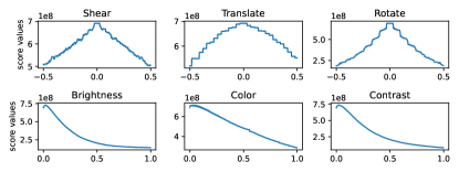
Figure 1: The score values - magnitude of augmentation graph for each transform which are sampled from RandAugment [10].

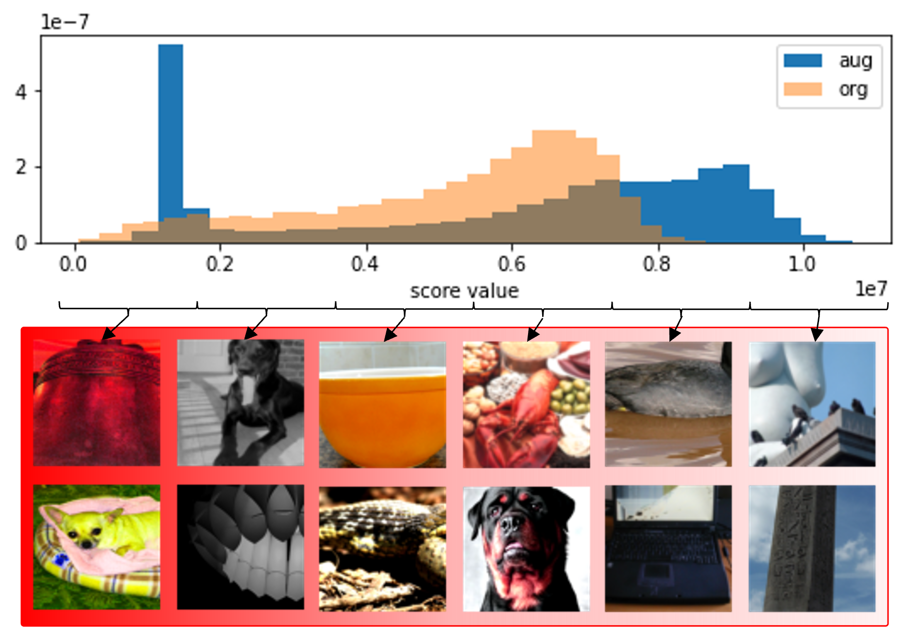
Figure 2: The histogram of score values and sample images in the binning range. We confirm that, unlike the distribution of the score values of the original image, that of augmented images has a peak. Through the qualitative analysis, we confirm that the transformed images with high intensity of augmentation (especially, color-related transform) have low score values as shown in the left two columns.

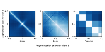
Figure 3: The relationship between the difference of score values and that of augmentation scale is illustrated in this figure, where brighter colors correspond to smaller differences. As indicated by the heatmap, we observe that the difference in score values decreases as the degree of transformation becomes closer. For instance, when both views undergo a “color” transformation (in the second column), if the magnitude increase is the same, the score value difference is low; conversely, if the difference in magnitude is large, the score difference also increases. It should be noted that the ‘Shear’ transform has a negative direction, so we align the original images (i.e. zero magnitudes) in the middle across the axis.

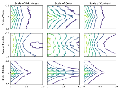
Figure 4: Contour map of score values when two augmentations are applied to one image. Each axis corresponds to the augmentation scale. We can confirm the non-linear relation between score values and augmentation scale when more than two transforms are applied to one images.

Contrastive Representation Learning. CL is a general framework for learning encoders so that the distance between positive pairs is close and the distance between negative pairs is far. Positive pairs are typically two views with one image undergoing transformations sampled randomly from the same data augmentation pool [5, 17, 16], but they are also defined as data within the same class or sequence [25, 19, 39]. Consider a dataset $\mathcal{D}=\{x_{i}|x_{i}\in\mathbb{R}^{n},i\in\mathcal{I}\}$. Let $z_{i}$ be an embedding vector of $x_{i}$ and $x_{i}^{+}$ be the positive pair of $x_{i}$ for which we desire to have similar representations. The similarity between them is obtained by the inner product and it is input to InfoNCE loss for CL:

$$L_{CL}=-\sum_{i}\log\dfrac{\exp(z_{i}^{T}\cdot z_{i}^{+}/\tau)}{\sum_{\gamma\in\Gamma(i)}exp(z_{i}^{T}\cdot z_{\gamma}/\tau)},$$ (4)

where $\Gamma(i)\equiv\mathcal{I}\setminus\{i\}$ and $\tau\in R^{+}$ is the scalar temperature hyperparameter. The denominator encourages the model to distinguish between $x_{i}$ and samples that are not positive pairs. Because this process is expensive in computing resources, a method for learning representations using only numerators (i.e. only positive pairs) has been proposed [7, 58, 2], which implies that a sampling method for positive pairs is a crucial part in CL [41].

3.2 Observation

Our work aims to make CL loss adaptively use the difference in the augmentation scale of views. Here, we present observations for supporting that the score matching function can estimate this degree. Note that in the previous section, the score value can be viewed as the output of a function that measures the level of noise embedded in the input image. Here we found two observations: 1) the stochastic coarse-to-fine gradient ascent procedure generalizes even in constrained sampling [23] and 2) the Gaussian noise-based image degradation plays a similar role in diffusion models with other augmentations (even completely deterministic degradation, e.g., blur masking and more) [1, 46]. Referring to them, we hypothesize that the score values for the augmented samples would be related to the corresponding noise level.

To show this, we investigate the variation in the output of score matching function according to the augmentation and make the following observations: 1) The strength of augmentation and the score value (the magnitude of the score matching function) are correlated. 2) The difference in the score values between the two augmented views is correlated with the difference in the augmentation scale applied to an image. 3) When two or more augmentations are sequentially applied, the score value is expressed as a non-linear combination of their intensities.

Analysis on score values. As illustrated in Figs. 1-4, we analyze the relationship between score values and augmentation strength. Since we use DSM [53] whose output is $\frac{(x-\tilde{x})}{\sigma^{2}}=-\frac{\epsilon}{\sigma}$ where $\tilde{x}=x+\sigma\epsilon$ and $\epsilon\sim\mathcal{N}(0,\sigma^{2})$, if the degree of deformation ($\sigma$) of the image is large, the absolute value of the score matching function output (score value) will be small.

1) Score values have a correlation with the strength of single augmentation. We first analyze how the score values of augmented samples change according to the strength of augmentation which is applied to the image. Figure 1 shows that the score value tends to decrease as the strength of augmentation increases. For the qualitative analysis, we plot the Fig. 2 which shows the histogram of score values obtained from ImageNet dataset [12] with RandAugment [10]. Images in the left two columns with small score values are deformed with color-related augmentation such as color jittering or grayscale. From these, we confirm that score values and the strength of augmentation are negatively correlated.

2) Gap of score values have a correlation with the strength gap between two different augmentations. For using the score values for the CL objective, the score value should also be related to augmentations applied to make two views. Therefore, we investigate the difference in score values of the two views that are produced by various augmentation strengths from the image. As shown in Fig. 3, the difference of score values is small if the scale of augmentation is similar, and vice versa. Through this, we conjecture that the difference of score values of the two views is correlated with the difference of the scale of augmentation. More various case studies are illustrated in appendix.

3) Score values have a non-linear correlation with the strength of a combination of multiple augmentations. From the above observations, one might design the adaptive CL objective by naively utilizing the difference in the scale of applied augmentation instead of using the score values. However, multiple augmentation methods can be sequentially applied to generate views and it is difficult to estimate the strength of these composited augmentations by the simple linear combination of each augmentation strength. Therefore, we analyze the expressivity of the score matching function when two augmentations are applied and illustrate this in Fig. 4. The results show that the score value is expressed as a non-linear combination of their intensities.

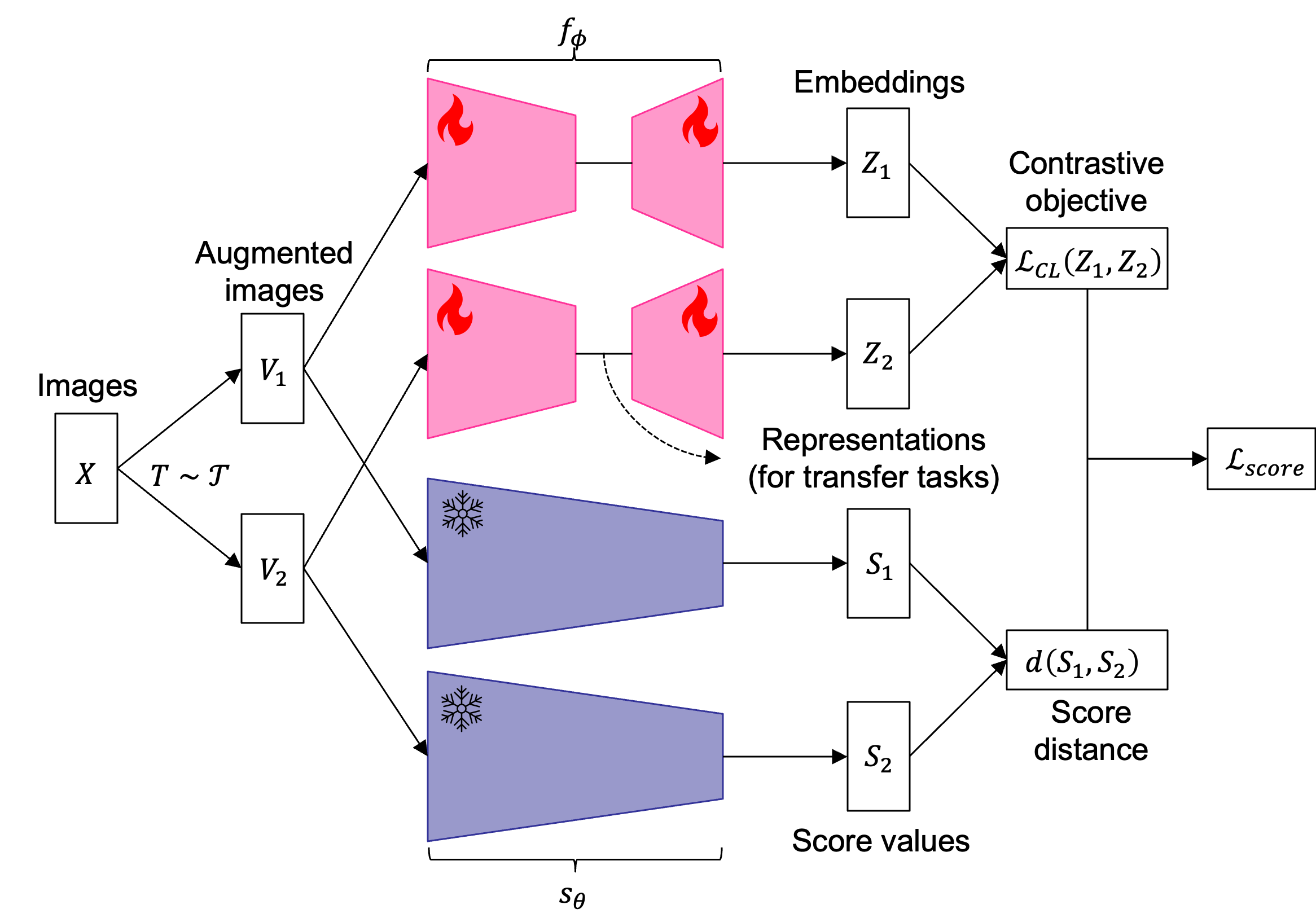
Figure 5: The architecture of ScoreCL with score matching function. The red diagram acts as the original CL model and the blue figure represents score guiding; it can represent the existing CL method with $d(S_{1},S_{2})=1$. Note that the $s_{\theta}$ is trained before CL so as to prevent the gradient flow through score matching.

3.3 Score-Guided Contrastive Learning

From the above observations, the score matching function can be used to estimate the difference in the strength of transforms applied to each view, we can design a CL objective that adaptively takes this into account. We first formulate the CL objective incorporating recent findings that a positive pair with a wide range of diversity enables representation learning more transferable, more stable converged, and leads to performance enhancement [52, 54, 55].

With attenuate weight $d(A(x_{i}),A(x_{i}^{+}))$ where $A(\cdot)$ is a mapping function from images to augmentation scale and $d(\cdot,\cdot)$ is a function to measure the distance between them, adaptive version of InfoNCE loss is represented as follows:

$$L_{A-CL}=$$ (5)

$$-\sum_{i}\log\dfrac{d(A(x_{i}),A(x_{i}^{+}))\exp(z_{i}^{T}\cdot z_{i}^{+})/\tau)}{\sum_{\gamma\in\Gamma(i)}d(A(x_{i}),A(x_{\gamma}))\exp(z_{i}^{T}\cdot z_{\gamma}/\tau)}.$$

This proposed adaptive loss puts more weight on learning pairs with a large difference in the augmentation strength.

For estimating the function $A(\cdot)$, existing works [20, 54] only focus on finding the impact of differences in augmentation scale with hand-crafted manner. Furthermore, these hand-crafted augmentation scales are globally fixed, resulting in the lack of pair-wise estimation. To overcome this limitation, we propose a score-guided CL that learns adaptively to attenuate hard positives by utilizing the characteristic of the score values. From the above observations, we set $A(\cdot)$ in equation 5 as $s_{\theta}(\cdot)$. We set $d$ as the L1 norm, and confirm that even when $d$ is set to the L2 norm, results similar to those analyzed above are obtained.

Our proposed method to utilize score values is illustrated in Fig. 5. The PyTorch-style pseudocode is shown in the appendix. To verify the generality of our approach to existing CL methods, we apply ours to four models: SimCLR, SimSiam, W-MSE, and VICReg. Note that our method can be applied to every CL method orthogonally to the usage of negative samples and improve the baselines consistently. The modified loss functions for each method are as follows:

• SimCLR [5]:

  $$-\log\frac{d(s_{\theta}(x_{i}),s_{\theta}(x_{i}^{+}))\exp(\text{sim}(z_{i},z_{i}^{+})/\tau)}{\sum_{\gamma\in\Gamma(i)}d(s_{\theta}(x_{i}),s_{\theta}(x_{\gamma}))\exp(z_{i}^{T}\cdot z_{\gamma}/\tau)}.$$ (6)

• SimSiam [7]:

  $$\frac{1}{2}d(s_{\theta}(x_{1}),s_{\theta}(x_{2}))(\mathcal{D}(p_{1},z_{2})+\mathcal{D}(p_{2},z_{1})),$$ (7)

  where $p$ is a representation from $z$ passing through prediction MLP head and $\mathcal{D}(x,y)=-\frac{x}{||x||_{2}}\cdot\frac{y}{||y||_{2}}$.

• W-MSE [13]:

  $$\frac{2}{Nm(m-1)}\Sigma d(s_{\theta}(x_{i}),s_{\theta}(x_{j}))dist(w_{i},w_{j}),$$ (8)

  where $N$ is the number of given original images, $k$ is a batch size, $m=K/N$, $w$ is a whitened vector from $z$.

• VICReg [2]:
  

  $$\lambda s_{score}(Z,Z^{\prime})+\mu[v(Z)+v(Z^{\prime})]+\nu[c(Z)+c(Z^{\prime})],$$ (9)

  where $\lambda,\mu$, and $\nu$ are hyper-parameters balancing the importance of each term. $s_{score}(Z,Z^{\prime})=\frac{1}{n}\Sigma_{i}d(s_{\theta}(x_{i}),s_{\theta}(x_{i}^{\prime}))||z_{i}-z_{i}^{\prime}||_{2}^{2}$ is invariance criterion. $v(Z)=\frac{1}{d}\Sigma_{j=1}^{d}\max(0,1-S(z^{j},\epsilon))$ is variance regularization where $S(x,\epsilon)=\sqrt{\text{Var}(x)+\epsilon}$, and the vector of each value of dimension $j$ as $z^{j}$ in all vectors in $Z$. $c(Z)=\frac{1}{d}\Sigma_{i\neq j}|C(Z)|^{2}_{i,j}$ is covariance regularization.

Training score matching model

Before learning representation in CL, we first pre-train the score matching using equation 3. As following [48], since $\mathcal{L}_{\sigma}$ relies on the scale of $\sigma$, we use unified objective with all $\sigma\in\{\sigma_{i}\}_{i=1}^{L}$ as follows:

$$\mathcal{L}_{s}=\frac{1}{L}\Sigma_{i=1}^{L}\lambda(\sigma_{i})\mathcal{L}_{\sigma},$$ (10)

where $\lambda(\sigma)=\sigma^{2}$ to derive $||\sigma s_{\theta}(\tilde{x})||_{2}\propto 1$. In fact, our method increases training cost, but it is minuscule since the score matching function and CL are trained separately. We discuss it more in the Appendix.

Method	Arch.	ImageNet-100
		base	score
SimCLR	ResNet-50	69.24	72.26(+3.02)
SimCLR	ResNet-101	70.14	72.90(+2.76)
SimSiam	ResNet-50	73.24	74.18(+0.94)
SimSiam	ResNet-101	74.02	75.04(+1.02)
VICReg	ResNet-50	70.24	71.44(+1.20)
VICReg	ResNet-101	71.56	72.24(+0.68)

Table 1: The classification accuracy of a 5-NN classifier for ImageNet-100 dataset and different CL. ScoreCL enhances the performance of all baseline CL methods.

Method	CIFAR-10		CIFAR-100
	base	score	base	score
SimCLR	90.28	91.01(+0.73)	60.11	62.34(+2.23)
SimSiam	90.27	90.80(+0.53)	63.15	64.55(+1.40)
W-MSE	90.06	91.35(+1.29)	56.69	56.94(+0.25)
VICReg	88.94	89.49(+0.55)	59.95	61.53(+1.58)

Table 2: The classification accuracy of a 5-NN classifier for different CL and datasets with ResNet-18 encoder. This demonstrates the generalizability of ScoreCL, as it enhances the performance of all baseline CL methods.

4 Experiments

4.1 Setup

Datasets and CL Models. To verify the consistent superiority of the proposed method, experiments have been conducted on various datasets and existing CL models. We use well-known benchmark datasets such as CIFAR-10, CIFAR-100 [28], and ImageNet-100 [12, 39] for training CL models such as SimCLR [5], SimSiam [7], W-MSE [13], and VICReg [2]. Further details such as hyperparameters are described in the appendix.

Image Augmentation. As Chen et al. [5] did, we extract crops with a random size from 0.2 to 1.0 of the original size and also apply horizontal mirroring with probability 0.5. Color jittering with configuration (0.4, 0.4, 0.4, 0.1) with probability 0.8 and grayscaling with probability 0.2 are applied too. For ImageNet-100, we add Gaussian blurring with a probability of 0.5.

Method	k-NN classifier						Linear classifier
SimSiam	STL10	Food	Flowers	Cars	Aircraft	DTD	STL10	Food	Flowers	Cars	Aircraft	DTD
base	80.56	46.31	61.60	16.03	21.57	54.57	87.79	59.07	64.04	26.96	25.33	55.85
score	83.04	45.97	64.55	16.23	21.48	56.09	88.79	59.34	66.03	25.46	26.77	57.28

Table 3: Transfer learning performance on object classification datasets. For Aircraft and Flowers, we report average per-class accuracy and top-1 for others. Note that we tune the hyperparameters of linear classifiers only with learning rates of 10, 30, 50, 70, and 90. Thus, the results of the linear classifier do not match those in the previous works, but ours almost always outperforms the baseline.

Method	VOC07+12			COCO detection			COCO segmentation
SimSiam	$\text{AP}_{\text{all}}$	$\text{AP}_{\text{50}}$	$\text{AP}_{\text{75}}$	$\text{AP}^{\text{bb}}$	$\text{AP}_{\text{50}}^{\text{bb}}$	$\text{AP}_{\text{75}}^{\text{bb}}$	$\text{AP}^{\text{mk}}$	$\text{AP}_{\text{50}}^{\text{mk}}$	$\text{AP}_{\text{75}}^{\text{mk}}$
base	53.8673	79.8484	59.5117	39.1496	59.0260	42.8220	34.3328	55.5996	36.6267
score	53.9903	80.2120	59.6897	39.9247	59.6728	43.1278	34.8430	56.2989	37.1830

Table 4: The results on object detection downstream task on VOC07+12 using Faster R-CNN [43] and in the detection and instance segmentation task on COCO using Mask R-CNN [18]. The detector for the VOC dataset is fine-tuned on trainval VOC07+12 and tested on test VOC07. The experiment is done by using MoCo [17] official implementation, which is based on Detectron2 [56].

Evaluation Protocol. The most common and reliable evaluation protocol for unsupervised representation learning is based on freezing the backbone network after CL, and then obtaining the accuracy of a k-nearest neighbors (K-NN) classifier (generally, $k=5$). It is a convenient and reliable evaluation metric because no additional training hyperparameters is required.

4.2 Quantitative Evaluation

Image Classification. Table 1 shows the results of the experiments on ImageNet-100 dataset for various CL methods. The CL, which learns with score-based weight, outperforms the model without it since score matching-based learning enables the CL encoder to be robust by adaptively considering the view pairs. Especially, on SimCLR and Simsiam, ResNet-50 learned with score outperforms baseline of ResNet-101 even though the number of parameters is smaller. Due to the out-of-memory issue, we could not report the results on W-MSE. The experimental results on small datasets are shown in Table 2 which shows the consistent increase in performance by applying the score-based penalty on the original contrastive objective. The results on ImageNet-1K are shown in the appendix.

Model	Base	Random	Pixel	Saliency	LPIPS	Score
SimCLR	60.11	60.08	59.39	60.59	60.11	62.34
Simsiam	63.15	56.37	63.02	63.76	61.99	64.55

Table 5: The comparison results with other weighted CL baselines on the CIFAR-100 dataset.

Method	bs	Augmentation
		(C,C)	(C,R)	(C,R)+score
SimCLR	128	57.39	60.12	63.03(+2.91)
	256	59.16	61.97	64.68(+2.71)
	512	60.11	63.06	65.26(+2.20)
SimSiam	128	62.08	65.63	66.18(+0.55)
	256	63.15	66.91	67.70(+0.79)
	512	61.76	65.91	67.06(+1.15)

Table 6: The ablation study on different augmentation processes for different batch sizes (bs) and CL on CIFAR-100 dataset. The ‘C’ represents the customized augmentation as introduced in section 4.1 and the ‘R’ means RandAugment [10]. $(X,Y)$ shows that $X$ augmentation is applied for one view and $Y$ for the other one.

Augmentation	CIFAR-10		CIFAR-100
	base	score	base	score
RandomCrop	90.40	90.94	63.86	64.03
ContrastiveCrop	90.72	90.99	64.47	64.56

Table 7: Linear classification results on SimSiam with ResNet-18 for different datasets and contrastive objective. We set the experimental setting such as linear evaluation protocol or augmentation strategies as in [40].

Transfer Learning. To evaluate the generalizability of the learned representation, we conduct transfer learning on a variety of different fine-grained datasets. For the image classification task, we follow the k-NN and linear evaluation protocols on the benchmark datasets such as STL10 [9], Food101[3], Flowers102 [38], StanfordCars [27], Aircraft [35], and DTD [8]. For linear evaluation, we train a classifier on the top of frozen representations of ResNet-50 trained in SimSiam as done in the previous works [16, 30, 6]. The results are in Table 3. Note that ScoreCL improves baseline in four out of six datasets in k-NN classification and five out of six datasets in linear evaluation, especially showing superior k-NN classification performance on Flowers102 (+2.9%p), and DTD (+1.5%p).

Also, we evaluate the trained representation by object detection and instance segmentation task. Following the setup in [17], we use the VOC07+12 [14] and COCO [31] datasets. The experimental results in Table 4 show that ScoreCL makes the existing CL methods enhanced for localization tasks as well.

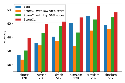
Figure 6: The ablation study on score thresholding with CIFAR-100 dataset. The integer numbers ‘128’, ‘256’, and ‘512’, indicate the batch size.

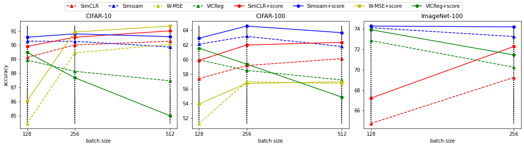
Figure 7: The ablation study on batch size for different datasets and CL models. The name with ’+score’ indicates the score-guided CL. Almost all performance increase when ours are applied.

4.3 Extensive Analysis

Comparison with Adaptive CL Baselines. With the analysis in Fig. 4, naively using the augmentation scale can’t make representation better when multiple augmentations are applied, so we use score values for estimating it. However, some naive baselines for measuring the difference between views can be replaced with score values. Instead of the score value, the followings are experimented with as the weight$A(\cdot)$ and are shown in Table 5: random, pixel-wise distance, saliency map (reflecting the task-relevant feature), and LPIPS (measuring the perceptual similarity) [59].

Comparison over various augmentations. Table 6 shows the results of proving that the proposed strategy adaptively penalizes the contrastive objective for any augmentation. When we apply different augmentation methods to each view as [54] (i.e., we enforce two views to be different), the performance increases on any batch size and CL models as is well known. This shows that our method could boost performances regardless of augmentation strategies.

Ablation on False Positive Pair. One may point out that false positive issues may arise, whereby an improperly augmented view is wrongly identified as a positive pair, for example, cropping the background without an object, yet treating it as a positive pair [41, 36, 40]. We thus test whether our method can perform robustly with ContrastiveCrop [40], which is proposed to solve the false positive problem. If our method assigns more penalties to the false positives, it may cause the ContrastiveCrop to fail. However, as shown in Table 7, there are further improvements when ScoreCL is applied even when ContrastiveCrop is used: it can boost performance due to its add-on property.

Ablation on Sampling Strategy. Unlike previous works that only use pairs of views having a large view variance, our method uses both large and small view variance pairs by penalizing the contrastive objective, which can make CL adaptively use a wide range of samples. Here, we validate the effectiveness of this adaptive utilization scheme for a better understanding of our method. To simulate that the only views with a large difference between variances are used to train CL, we sample the batch twice and use half of them by thresholding the scores with the median of score values of sampled batch data. The results illustrated in Fig. 6 show that the score distance-agnostic method with a wide range of augmentation outperforms others only with a biased range.

Ablation on Batch Size. Depending on batch size, the performance of CL can be dramatically varied [5]. Considering this, we investigate whether our method is effective for various batch sizes. As illustrated in Fig. 7, even under any batch size condition except for VICReg on CIFAR-10 and CIFAR-100 datasets, it is shown that the performance is consistently enhanced when the score is applied to the existing CL. In the case of VICReg, it seems to be an unintended result because the variance regularizer can adversely affect training when images of the same class fit into one batch.

5 Conclusion & Discussion

In this paper, we propose a novel and simple method to learn better representation in CL with a score matching function. We address the problem that there is no work on a contrastive objective considering the variance difference between augmented images even though there are studies that such a distance is good for CL. To the best of our knowledge, it is the first work to analyze the property of the score matching function by relating them with the magnitude of augmentation. Based on this observation, we define the score-matching guided contrastive learning to adaptively consider the view variance, ScoreCL, and conduct several experiments to verify the consistent performance increase regardless of datasets, augmentation strategy, or CL models. As a result, when our strategy is applied to the existing methods, we can obtain a better representation in the viewpoint of classification accuracy of a 5-nearest neighbors classifier. To deal with the false positive problem which is one of the challenges of augmentation in CL, we also adapt our method to ConstrastCrop and obtain improved performance. Furthermore, our methods outperform baselines on transfer learning for object classification and downstream detection tasks.

In order to overcome the limitation of showing only experimental evidence for the hypothesis about the score, we will verify the inferred property of score matching through theoretical analysis. In addition, by applying a universal augmentation technique and using an augmentation-agnostic proposed method, we want to provide a future direction that only needs to consider a contrastive objective among the significant components of CL.

A. Score Analysis

The augmentations written in the top and left in Fig. 8 are applied in each view, respectively. For example, the image in the first row and the fifth column is a heatmap of the difference in score values from two images which are augmented with ‘Shear’ and ‘Color’ augmentation, respectively. As we mentioned, note that the magnitude of ‘Shear’ augmentation is aligned in the middle across the y-axis. In the middle of the y-axis, where ‘Shear’ is hardly applied, the difference in score values increases according to the strength of ‘Color’, whereas the opposite trend appears after ‘Shear’ is applied to some extent. It can be interpreted that the distance from the true distribution is rather far, so the difference between the two gradients (score values) is recognized as small. Otherwise, the case where the relationship between the difference in score value and the difference in augmentation strength can be most easily confirmed is in the third row and eighth column (i.e., when the “Posterize” transform is applied to each of the two images).

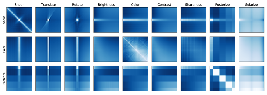
Figure 8: The observation that the difference of score value is related to that of augmentation-scale. Note that the “Shear”, and “Translate” transforms have negative directions, so we align the original images (i.e. zero magnitudes) in the middle across the axis. We can find that the difference in score values is smaller as the degree of transforms is closer. For example, when both views are transformed with “Color” (at the second row and fifth column), if the magnitude increases to the same degree, the difference between score values is low, and if the difference in magnitude is large, the difference in score is also increased.

B. Implementation Details

For a SimCLR and SimSiam, we use the SGD optimizer with momentum 0.9 [50]. For W-MSE and VICReg, we follow the official settings: Adam and LARS optimizers [26, 57], respectively. Specifically, on CIFAR-10 and CIFAR-100 datasets, for SimCLR, we train CL for 1,000 epochs with a learning rate 0.5, weight decay 0.0001, and temperature 0.5; for SimSiam, 1,000 epochs with a learning rate 0.06 and weight decay 0.0005; for W-MSE, 1,000 epochs with learning rate 0.001 and weight decay $10^{-6}$. On ImageNet datasets, for SimCLR, the model learns for 200 epochs with learning rate 0.5, weight decay 0.0001, and temperature 0.5; for SimSiam, 200 epochs with a learning rate 0.1 and weight decay 0.0001. Also, we use a cosine learning rate decay with 10 epochs warm-up for all experiments. The embedding size and hyperparameters configuration is set as that of the original paper. The PyTorch-style pseudocode is shown in Algorithm 1.

Algorithm 1 PyTorch-style pseudocode for ScoreCL

1:  Input: An encoder network $f_{\phi}$, a score matching $s_{\theta}$, contrative objective $\mathcal{L}_{CL}$, and distance measure $d$

2:  for $x$ in loader:

3:     $v_{1}$, $v_{2}$ = augment$(x)$

4:     # compute embeddings

5:     $z_{1},z_{2}=f_{\phi}(v_{1}),f_{\phi}(v_{2})$

6:     # compute score values

7:     $s_{1},s_{2}=s_{\theta}(v_{1}),s_{\theta}(v_{2})$

8:     # obtain loss for contrastive learning

9:     cl_loss = $\mathcal{L}_{CL}(z_{1},z_{2})$

10:     # obtain distance between scores from views

11:     score_dist = $d(s_{1},s_{2})$

12:     # scoreCL

13:     loss = (score_dist.detach() * cl_loss).mean(0)

14:     # optimizatin step

15:     loss.backward()

16:     optimizer.step()

C. Experiments on Large-scale Dataset

The experiment on the large-scale dataset such as ImageNet-1K is conducted to verify the consistent improvements when our method is applied. As shown in Table 8, the performance increases when we exploit the score-matching function on ImageNet-1K dataset as well as CIFAR-10, CIFAR-100, and ImageNet-100 datasets.

Classifier	SimCLR		Simsiam		VICReg
	base	score	base	score	base	score
k-NN	42.62	45.59	54.66	54.98	55.08	57.80
Linear	56.98	59.21	58.13	59.98	59.58	61.86

Table 8: The classification accuracy of 5-NN and linear classifiers on ImageNet-1K dataset and different CL with ResNet-50 encoder.

D. Experiments on Different Arichitecture

We conducted experiments using various architectures, including the Vision Transformer (ViT), to validate the consistent improvements achieved by our method. Table 9 demonstrates that our approach enhances performance when applied to both ViT and ResNet, utilizing the score-matching function.

SimCLR	ViT-S/4	ViT-S/8	ViT-S/16	ViT-B/8	ViT-B/16
base	58.49	55.51	47.11	55.87	47.11
score	60.91	58.01	50.44	59.17	48.56

Table 9: The classification accuracy of a 5-NN classifier with ViT-S & -B on CIFAR-100 dataset. The “/$N$” means the size of the patch.

E. Analysis on Training Cost

The proposed score-guided CL has two training phase: score-matching function and CL. It is true that ours increases training cost, but it is minuscule since the score-matching function and CL are trained separately. We show the number of parameters and performance in Table 11. Comparing “ResNet50+score” and “ResNet101” in each method, applying the proposed method achieves better performance even though there are fewer parameters of about 18M. Note that the number of parameters in score mathcing function is about 1.8M and they are trained separately from CL. Besides, Table 10 shows the performance of ‘base+’ learned for the same amount of time as scoreCL.

Model	Base	Base+	Score
SimCLR	60.11	60.91	62.34(+1.43)
Simsiam	63.15	63.32	64.55(+1.23)

Table 10: The performance of CLs with fair training time.

Method	Arch.	Weight	Param.	Acc.
SimCLR	ResNet50	base	32.16M	69.24%
		score	33.54M	72.26%
	ResNet101	base	51.16M	70.14%
		score	52.53M	72.90%
Simsiam	ResNet50	base	38.21M	73.24%
		score	39.59M	74.18%
	ResNet101	base	57.20M	74.02%
		score	58.58M	75.04%

Table 11: Comparison of the number of parameters and performance on ImageNet-100 dataset.

F. Negative Impacts

Our proposed methods make CL model focus on the difference between the views to cover a wide range of view diversity. However, ScoreCL can fall into the risk of assigning the penalty considering only differences in augmentation regardless of the real class of images. It implies that the representation of CL used in multiple downstream tasks can be collapsed, which can adversely affect other applications. To overcome this, class-specific methods, as well as augmentation scale-agnostic approach, should be studied as we do in section 4.3.

References

- [1] Arpit Bansal, Eitan Borgnia, Hong-Min Chu, Jie S Li, Hamid Kazemi, Furong Huang, Micah Goldblum, Jonas Geiping, and Tom Goldstein. Cold diffusion: Inverting arbitrary image transforms without noise. arXiv preprint arXiv:2208.09392, 2022.
- [2] Adrien Bardes, Jean Ponce, and Yann LeCun. Vicreg: Variance-invariance-covariance regularization for self-supervised learning. arXiv preprint arXiv:2105.04906, 2021.
- [3] Lukas Bossard, Matthieu Guillaumin, and Luc Van Gool. Food-101–mining discriminative components with random forests. In European conference on computer vision, pages 446–461. Springer, 2014.
- [4] Mathilde Caron, Ishan Misra, Julien Mairal, Priya Goyal, Piotr Bojanowski, and Armand Joulin. Unsupervised learning of visual features by contrasting cluster assignments. Advances in Neural Information Processing Systems, 33:9912–9924, 2020.
- [5] Ting Chen, Simon Kornblith, Mohammad Norouzi, and Geoffrey Hinton. A simple framework for contrastive learning of visual representations. In International conference on machine learning, pages 1597–1607. PMLR, 2020.
- [6] Xinlei Chen, Haoqi Fan, Ross Girshick, and Kaiming He. Improved baselines with momentum contrastive learning. arXiv preprint arXiv:2003.04297, 2020.
- [7] Xinlei Chen and Kaiming He. Exploring simple siamese representation learning. In Proceedings of the IEEE/CVF Conference on Computer Vision and Pattern Recognition, pages 15750–15758, 2021.
- [8] M. Cimpoi, S. Maji, I. Kokkinos, S. Mohamed, , and A. Vedaldi. Describing textures in the wild. In Proceedings of the IEEE Conf. on Computer Vision and Pattern Recognition (CVPR), 2014.
- [9] Adam Coates, Andrew Ng, and Honglak Lee. An analysis of single-layer networks in unsupervised feature learning. In Proceedings of the fourteenth international conference on artificial intelligence and statistics, pages 215–223. JMLR Workshop and Conference Proceedings, 2011.
- [10] Ekin D Cubuk, Barret Zoph, Jonathon Shlens, and Quoc V Le. Randaugment: Practical automated data augmentation with a reduced search space. In Proceedings of the IEEE/CVF conference on computer vision and pattern recognition workshops, pages 702–703, 2020.
- [11] J. Cui, Z. Zhong, S. Liu, B. Yu, and J. Jia. Parametric contrastive learning. In 2021 IEEE/CVF International Conference on Computer Vision (ICCV), pages 695–704, Los Alamitos, CA, USA, oct 2021. IEEE Computer Society.
- [12] Jia Deng, Wei Dong, Richard Socher, Li-Jia Li, Kai Li, and Li Fei-Fei. Imagenet: A large-scale hierarchical image database. In 2009 IEEE conference on computer vision and pattern recognition, pages 248–255. Ieee, 2009.
- [13] Aleksandr Ermolov, Aliaksandr Siarohin, Enver Sangineto, and Nicu Sebe. Whitening for self-supervised representation learning. In International Conference on Machine Learning, pages 3015–3024. PMLR, 2021.
- [14] Mark Everingham, Luc Van Gool, Christopher KI Williams, John Winn, and Andrew Zisserman. The pascal visual object classes (voc) challenge. International journal of computer vision, 88(2):303–338, 2010.
- [15] Ross Girshick, Jeff Donahue, Trevor Darrell, and Jitendra Malik. Rich feature hierarchies for accurate object detection and semantic segmentation. In Proceedings of the IEEE conference on computer vision and pattern recognition, pages 580–587, 2014.
- [16] Jean-Bastien Grill, Florian Strub, Florent Altché, Corentin Tallec, Pierre Richemond, Elena Buchatskaya, Carl Doersch, Bernardo Avila Pires, Zhaohan Guo, Mohammad Gheshlaghi Azar, et al. Bootstrap your own latent-a new approach to self-supervised learning. Advances in neural information processing systems, 33:21271–21284, 2020.
- [17] Kaiming He, Haoqi Fan, Yuxin Wu, Saining Xie, and Ross Girshick. Momentum contrast for unsupervised visual representation learning. In Proceedings of the IEEE/CVF conference on computer vision and pattern recognition, pages 9729–9738, 2020.
- [18] Kaiming He, Georgia Gkioxari, Piotr Dollár, and Ross Girshick. Mask r-cnn. In Proceedings of the IEEE international conference on computer vision, pages 2961–2969, 2017.
- [19] Olivier Henaff. Data-efficient image recognition with contrastive predictive coding. In International conference on machine learning, pages 4182–4192. PMLR, 2020.
- [20] Weiran Huang, Mingyang Yi, and Xuyang Zhao. Towards the generalization of contrastive self-supervised learning. arXiv preprint arXiv:2111.00743, 2021.
- [21] Aapo Hyvärinen. Optimal approximation of signal priors. Neural Computation, 20(12):3087–3110, 2008.
- [22] Aapo Hyvärinen, Jarmo Hurri, and Patrik O Hoyer. Estimation of non-normalized statistical models. In Natural Image Statistics, pages 419–426. Springer, 2009.
- [23] Zahra Kadkhodaie and Eero Simoncelli. Stochastic solutions for linear inverse problems using the prior implicit in a denoiser. Advances in Neural Information Processing Systems, 34:13242–13254, 2021.
- [24] Yannis Kalantidis, Mert Bulent Sariyildiz, Noe Pion, Philippe Weinzaepfel, and Diane Larlus. Hard negative mixing for contrastive learning. Advances in Neural Information Processing Systems, 33:21798–21809, 2020.
- [25] Prannay Khosla, Piotr Teterwak, Chen Wang, Aaron Sarna, Yonglong Tian, Phillip Isola, Aaron Maschinot, Ce Liu, and Dilip Krishnan. Supervised contrastive learning. Advances in Neural Information Processing Systems, 33:18661–18673, 2020.
- [26] Diederik P Kingma and Jimmy Ba. Adam: A method for stochastic optimization. arXiv preprint arXiv:1412.6980, 2014.
- [27] Jonathan Krause, Michael Stark, Jia Deng, and Li Fei-Fei. 3d object representations for fine-grained categorization. In Proceedings of the IEEE international conference on computer vision workshops, pages 554–561, 2013.
- [28] Alex Krizhevsky, Geoffrey Hinton, et al. Learning multiple layers of features from tiny images. 2009.
- [29] Alex Krizhevsky, Ilya Sutskever, and Geoffrey E Hinton. Imagenet classification with deep convolutional neural networks. Communications of the ACM, 60(6):84–90, 2017.
- [30] Kyungmin Lee and Jinwoo Shin. R’enyicl: Contrastive representation learning with skew r’enyi divergence. arXiv preprint arXiv:2208.06270, 2022.
- [31] Tsung-Yi Lin, Michael Maire, Serge Belongie, James Hays, Pietro Perona, Deva Ramanan, Piotr Dollár, and C Lawrence Zitnick. Microsoft coco: Common objects in context. In European conference on computer vision, pages 740–755. Springer, 2014.
- [32] Jonathan Long, Evan Shelhamer, and Trevor Darrell. Fully convolutional networks for semantic segmentation. In Proceedings of the IEEE conference on computer vision and pattern recognition, pages 3431–3440, 2015.
- [33] Shuang Ma, Zhaoyang Zeng, Daniel McDuff, and Yale Song. Active contrastive learning of audio-visual video representations. arXiv preprint arXiv:2009.09805, 2020.
- [34] Ahsan Mahmood, Junier Oliva, and Martin Styner. Multiscale score matching for out-of-distribution detection. arXiv preprint arXiv:2010.13132, 2020.
- [35] S. Maji, J. Kannala, E. Rahtu, M. Blaschko, and A. Vedaldi. Fine-grained visual classification of aircraft. Technical report, 2013.
- [36] Sangwoo Mo, Hyunwoo Kang, Kihyuk Sohn, Chun-Liang Li, and Jinwoo Shin. Object-aware contrastive learning for debiased scene representation. Advances in Neural Information Processing Systems, 34:12251–12264, 2021.
- [37] Pedro Morgado, Nuno Vasconcelos, and Ishan Misra. Audio-visual instance discrimination with cross-modal agreement. In Proceedings of the IEEE/CVF Conference on Computer Vision and Pattern Recognition, pages 12475–12486, 2021.
- [38] Maria-Elena Nilsback and Andrew Zisserman. Automated flower classification over a large number of classes. In 2008 Sixth Indian Conference on Computer Vision, Graphics & Image Processing, pages 722–729. IEEE, 2008.
- [39] Aaron van den Oord, Yazhe Li, and Oriol Vinyals. Representation learning with contrastive predictive coding. arXiv preprint arXiv:1807.03748, 2018.
- [40] Xiangyu Peng, Kai Wang, Zheng Zhu, Mang Wang, and Yang You. Crafting better contrastive views for siamese representation learning. In Proceedings of the IEEE/CVF Conference on Computer Vision and Pattern Recognition, pages 16031–16040, 2022.
- [41] Senthil Purushwalkam and Abhinav Gupta. Demystifying contrastive self-supervised learning: Invariances, augmentations and dataset biases. Advances in Neural Information Processing Systems, 33:3407–3418, 2020.
- [42] Rui Qian, Tianjian Meng, Boqing Gong, Ming-Hsuan Yang, Huisheng Wang, Serge Belongie, and Yin Cui. Spatiotemporal contrastive video representation learning. In Proceedings of the IEEE/CVF Conference on Computer Vision and Pattern Recognition, pages 6964–6974, 2021.
- [43] Shaoqing Ren, Kaiming He, Ross Girshick, and Jian Sun. Faster r-cnn: Towards real-time object detection with region proposal networks. Advances in neural information processing systems, 28, 2015.
- [44] Joshua Robinson, Ching-Yao Chuang, Suvrit Sra, and Stefanie Jegelka. Contrastive learning with hard negative samples. arXiv preprint arXiv:2010.04592, 2020.
- [45] Olga Russakovsky, Jia Deng, Hao Su, Jonathan Krause, Sanjeev Satheesh, Sean Ma, Zhiheng Huang, Andrej Karpathy, Aditya Khosla, Michael Bernstein, et al. Imagenet large scale visual recognition challenge. International journal of computer vision, 115(3):211–252, 2015.
- [46] Jascha Sohl-Dickstein, Eric Weiss, Niru Maheswaranathan, and Surya Ganguli. Deep unsupervised learning using nonequilibrium thermodynamics. In International Conference on Machine Learning, pages 2256–2265. PMLR, 2015.
- [47] Jiaming Song and Stefano Ermon. Multi-label contrastive predictive coding. In H. Larochelle, M. Ranzato, R. Hadsell, M.F. Balcan, and H. Lin, editors, Advances in Neural Information Processing Systems, volume 33, pages 8161–8173. Curran Associates, Inc., 2020.
- [48] Yang Song and Stefano Ermon. Generative modeling by estimating gradients of the data distribution. Advances in Neural Information Processing Systems, 32, 2019.
- [49] Yang Song, Sahaj Garg, Jiaxin Shi, and Stefano Ermon. Sliced score matching: A scalable approach to density and score estimation. In Uncertainty in Artificial Intelligence, pages 574–584. PMLR, 2020.
- [50] Ilya Sutskever, James Martens, George Dahl, and Geoffrey Hinton. On the importance of initialization and momentum in deep learning. In International conference on machine learning, pages 1139–1147. PMLR, 2013.
- [51] Yonglong Tian, Dilip Krishnan, and Phillip Isola. Contrastive multiview coding. In European conference on computer vision, pages 776–794. Springer, 2020.
- [52] Yonglong Tian, Chen Sun, Ben Poole, Dilip Krishnan, Cordelia Schmid, and Phillip Isola. What makes for good views for contrastive learning? Advances in Neural Information Processing Systems, 33:6827–6839, 2020.
- [53] Pascal Vincent. A connection between score matching and denoising autoencoders. Neural computation, 23(7):1661–1674, 2011.
- [54] Xiao Wang, Haoqi Fan, Yuandong Tian, Daisuke Kihara, and Xinlei Chen. On the importance of asymmetry for siamese representation learning. In Proceedings of the IEEE/CVF Conference on Computer Vision and Pattern Recognition, pages 16570–16579, 2022.
- [55] Xiao Wang and Guo-Jun Qi. Contrastive learning with stronger augmentations. IEEE Transactions on Pattern Analysis and Machine Intelligence, 2022.
- [56] Yuxin Wu, Alexander Kirillov, Francisco Massa, Wan-Yen Lo, and Ross Girshick. Detectron2. https://github.com/facebookresearch/detectron2, 2019.
- [57] Yang You, Jing Li, Sashank Reddi, Jonathan Hseu, Sanjiv Kumar, Srinadh Bhojanapalli, Xiaodan Song, James Demmel, Kurt Keutzer, and Cho-Jui Hsieh. Large batch optimization for deep learning: Training bert in 76 minutes. arXiv preprint arXiv:1904.00962, 2019.
- [58] Jure Zbontar, Li Jing, Ishan Misra, Yann LeCun, and Stéphane Deny. Barlow twins: Self-supervised learning via redundancy reduction. In International Conference on Machine Learning, pages 12310–12320. PMLR, 2021.
- [59] Richard Zhang, Phillip Isola, Alexei A Efros, Eli Shechtman, and Oliver Wang. The unreasonable effectiveness of deep features as a perceptual metric. In Proceedings of the IEEE conference on computer vision and pattern recognition, pages 586–595, 2018.