Spin Squeezing with Arbitrary Quadratic Collective-Spin Interaction

Abstract

Spin squeezing is vitally important in quantum metrology and quantum information science. The noise reduction resulting from spin squeezing can surpass the standard quantum limit and even reach the Heisenberg Limit (HL) in some special circumstances. However, systems that can reach the HL are very limited. Here we study the spin squeezing in atomic systems with a generic form of quadratic collective-spin interaction, which can be described by the Lipkin-Meshkov-Glick(LMG) model. We find that the squeezing properties are determined by the initial states and the anisotropic parameters. Moreover, we propose a pulse rotation scheme to transform the model into two-axis twisting model with Heisenberg-limited spin squeezing. Our study paves the way for reaching HL in a broad variety of systems.

I Introduction

Squeezed spin states (SSSs) [1, 2] are entangled quantum states of a collection of spins in which the uncertainty of one spin component perpendicular to the mean spin direction is reduced below the standard quantum limit (SQL). Owing to its property of reduced spin fluctuations, it has a variety of applications in the study of many-body entanglement [3, 4, 5, 6, 7, 8, 9, 10, 11, 12], high-precision measurements [13, 14, 15, 16, 17, 18, 19], and quantum information science [20, 21, 22, 23]. Many methods have been proposed to realize spin squeezing, such as atom-light interaction [24], and quantum nondemolition measurement [25]. One important way to deterministically generate spin squeezing is utilizing the dynamical evolution of squeezing interaction, which is accomplished via collective-spin systems with nonlinear interaction [2]. Typical squeezing interactions include one-axis twisting (OAT) interaction and two-axis twisting (TAT) interaction. The noise reduction of the TAT model can reach the Heisenberg limit (HL), but the physical realization of the TAT model is difficult. It is shown that the OAT model can be transformed into TAT model using repeated Rabi pulses [26], but the more general cases with other types of quadratic collective-spin interaction are still unknown.

Except for OAT and TAT interactions, the more general form of quadratic collective-spin interaction can be described by the Lipkin-Meshkov-Glick (LMG) model. The LMG model was first introduced in nuclear physics [27, 28, 29, 30, 31, 32], which provides a simple description of the tunneling of bosons between two degenerate levels and can thus be used to describe many physical systems such as two-mode Bose-Einstein condensates [33] or Josephson junctions [34]. A recent study shows that the LMG model could be used in generating spin squeezing and having 6.8(4) dB metrological gain beyond the Standard Quantum Limit with suitable time-reversal control in cavity QED [35]. However, it requires a tunable Hamiltonian by switching to another set of laser frequencies on the cavity, which is not always accessible. A more general investigation of the LMG model in spin squeezing is required and whether it could reach Heisenberg-limited noise reduction remains unknown.

Here we study the spin squeezing properties in the LMG model with different anisotropic parameters. We find that initial state and the anisotropic parameter play important roles in the spin squeezing. We propose an implementable way to transform the LMG model into effective TAT model by making use of rotation pulses along different axes on the Bloch sphere, which gives a convenient way to generate efficient spin squeezing reaching the HL. We also analyze the influence of noises and find that our scheme is robust to fluctuations in pulse areas and pulse separations.

The paper is organized as follows. In Sec. (II), we first introduce the system model of the quadratic collective-spin interaction, which can be described by the LMG model. In Sec. (III), we investigate the performance of spin squeezing in the LMG mode and present the optimal initial state for spin squeezing in the LMG model. In Sec. (IV), we prove that the designed rotation pulse method can transform the LMG model into effective TAT interaction. We also show that the method is robust to different noises according to numerical simulations.

II THE SYSTEM MODEL

We consider a system of mutually interacting spin-1/2 particles described by the following Hamiltonian:

$$H=\sum_{j<k}\chi_{\alpha\beta}\sigma_{\alpha}^{j}\sigma_{\beta}^{k},$$ (1)

where $\sigma_{\alpha}^{j}$ is the Pauli operator of the $j$-th spin and $\alpha,\beta\in\{x,y,z\}$. The parameter $\chi_{\alpha\beta}$ characterize the strength of the interaction in different directions. To ensure the Hermicity of the Hamiltonian, we have $\chi_{\alpha\beta}=\chi_{\beta\alpha}$. Here we have the assumption that the interactions between individual spins are the same. This assumption holds when there are all-to-all interactions rather than just dipole-dipole interactions, which is valid under some systems such as nuclear system [29], Cavity QED [9], ion trap [10]. Now we introduce the collective spin operators $S_{\alpha}=\frac{\hbar}{2}\sum_{j}\sigma_{\alpha}^{j}$. Let $\hbar=1$, using

$$\sigma_{\alpha}\sigma_{\beta}=i\sum_{\gamma}\varepsilon_{\alpha\beta\gamma}\sigma_{\gamma}+\delta_{\alpha\beta},$$ (2)

where $\varepsilon_{\alpha\beta\gamma}$ is the Levi-Civita symbol and $\delta_{\alpha\beta}$ is the Kronecker delta, Eq. (1) becomes

$$H=2\sum_{\alpha,\beta\in\{x,y,z\}}\chi_{\alpha\beta}S_{\alpha}S_{\beta}+H_{0},$$ (3)

where $H_{0}$ is a constant and can be neglected. $H$ preserves the magnitude of the total spin $S^{2}=\sum_{\alpha}S^{2}_{\alpha}$, namely,

$$[H,S^{2}]=0,$$ (4)

which means $S^{2}$ is a constant. The Hamiltonian can be written as

$$H=\bm{S^{T}AS},$$ (5)

where $A_{\alpha\beta}=2\chi_{\alpha\beta}$. $\bm{A}$ is a real symmetric matrix, which means it can be diagonalized by a linear transformation:

$$\bm{A}=\bm{Q^{-1}DQ},$$ (6)

in which $\bm{Q}$ is an orthogonal matrix and $\bm{D}$ is a diagonal matrix whose nonzero elements are eigenvalues of $\bm{A}$. Let $\bm{\tilde{S}}=\bm{QS}$, we can turn the Hamiltonian into the canonical form:

$$H=\sum_{\alpha\in\{x,y,z\}}\chi_{\alpha}\tilde{S}_{\alpha}^{2},$$ (7)

For convenience, in the following we redefine the spin operator $S_{\alpha}$ by omitting the tilde. We select the corresponding $\tilde{S_{\alpha}}$ of the largest $\chi_{\alpha}$ as $S_{x}$ and the minimum as $S_{z}$, i.e., $\chi_{x}\geq\chi_{y}\geq\chi_{z}$. Using the relation $\sum_{\alpha}S^{2}_{\alpha}=S^{2}$, the transformed Hamiltonian reads

$$H=(\chi_{x}-\chi_{z})S_{x}^{2}+(\chi_{y}-\chi_{z})S_{y}^{2}+S^{2}.$$ (8)

Let $\chi=\chi_{x}-\chi_{z}$, $\gamma=(\chi_{y}-\chi_{z})/(\chi_{x}-\chi_{z})$ and ignore the constant term, we obtain the general form of the Hamiltonian of the LMG model

$$H=\chi(S_{x}^{2}+\gamma S_{y}^{2}).$$ (9)

Therefore, any system with Hamiltonian in the form of Eq. (1) can be transformed to the standard form of the LMG model as Eq. (9). What’s worth mentioning is that we ignore the linear interaction between the spin and external magnetic field. The reason is that linear interaction itself can’t generate spin squeezing, and the linear interaction could be easily canceled in the experimental system using suitable pulse sequences.

Under the condition $\chi_{x}\geq\chi_{y}\geq\chi_{z}$, we have $0\leq\gamma\leq 1$. Furthermore, note that if $0.5<\gamma\leq 1$, we have:

$$H=\chi(S_{x}^{2}+\gamma S_{y}^{2}-S^{2})=-\chi[S_{z}^{2}+(1-\gamma)S_{y}^{2}].$$ (10)

which is equivalent to $\chi[S_{x}^{2}+(1-\gamma)S_{y}^{2}]$ if we switch the $x$-axis and the $z$-axis. Hence, we only need to consider the situation when $0\leq\gamma\leq 0.5$. Specially, when $\gamma=0$ ($\gamma=0.5$), the LMG Hamiltonian reduces to the OAT (TAT) Hamiltonian.

III SPIN SQUEEZING OF THE LMG MODEL

To describe the properties of SSS, we investigate the squeezing parameter given by Kitagawa and Ueda [2]:

$$\xi^{2}=\frac{4(\Delta S_{\vec{n}_{\perp}})^{2}}{N},$$ (11)

where subscript $\vec{n}_{\perp}$ refers to an arbitrary axis perpendicular to the mean spin direction, where the minimum value of $(\Delta S)^{2}$ is obtained. The inequality $\xi^{2}<1$ indicates that the state is squeezed.

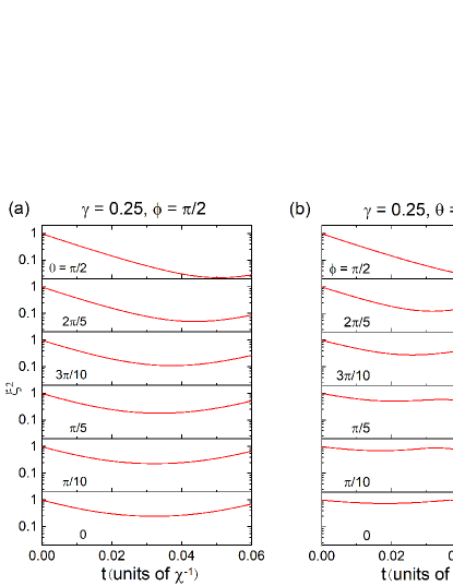
Figure 1: Time evolution of the squeezing parameter $\xi^{2}$ for anisotropic parameter $\gamma=0.25$ with different initial $\phi$ and $\theta$. (a) $\phi=\pi/2$ , $\theta$ changes from 0 to $\pi/2$. (b) $\theta=\pi/2$ , $\phi$ changes from 0 to $\pi/2$.

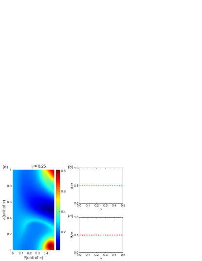
Figure 2: Minimum squeezing parameter $\xi^{2}$ as a function of the initial $\theta$ and $\phi$. (b)The optimal initial state azimuth angle $\phi_{0}$ when $\xi^{2}$ reaches its minimum in the condition of different $\gamma$. (c)The optimal initial state polar angle $\theta_{0}$ when $\xi^{2}$ reaches its minimum in the condition of different $\gamma$. The anisotropic parameter is $\gamma=0.25$.

The Hamiltonian of the LMG model is a typical kind of nonlinear interaction, which produces SSS by time evolution. We choose the coherent spin states as the initial states, which can be described by

$$\ket{\theta,\phi}=e^{i\theta(S_{x}\sin\phi-S_{y}\cos\phi)}\ket{j,j},$$ (12)

where $\theta$ is the angle between the $z$-axis and the collective-spin vector (polar angle), while $\phi$ is the angle between the $x$-axis and the vertical plane containing the collective-spin vector (azimuth angle).

Typical examples of the time evolution of $\xi^{2}$ are presented in Fig. 1. It reveals that the squeezing parameter reaches a local minimum in a short time scale. For a certain $\gamma$, the minimum squeezing parameter and the corresponding time varies with the initial $\theta$ and $\phi$.

In Fig. 2(a), we plot the color map of the minimum squeezing parameter as functions of the initial $\phi$ and $\theta$ for fixed $\gamma$ (for example, $\gamma=0.25$). It reveals that the optimal initial state with best squeezing is $\ket{\theta,\phi}=\ket{\pi/2,\pi/2}$. Similarly, we change $\gamma$ and plot the color maps, with the optimal initial $\phi$ and $\theta$ plotted in Fig. 2(b) and Fig. 2(c). We can see that when $\gamma$ varies from 0 to 0.5, the LMG model obtains the optimal squeezing when the initial state is $\ket{\pi/2,\pi/2}$. This can be understood in an intuitive sense: when $0\leq\gamma\leq 0.5$, we have:

$$H=\chi[(1-\gamma)S_{x}^{2}-\gamma S_{z}^{2}+\gamma S^{2}],$$ (13)

which can be seen as two counter-twisting squeezing acting around the $x$-axis and $z$-axis, respectively, and along the $y$-axis these two effects reach the optimal cases at the same time. Thus the optimal initial state is always $\ket{\pi/2,\pi/2}$.

Now we let the initial state be the optimal case $\ket{\pi/2,\pi/2}$, which could be realized through optical pumping and a $\pi/2$ pulse along the $x$-axis. And we track how the minimum squeezing parameter $\xi^{2}$ changes when $\gamma$ varies from 0 to 0.5. The results are shown in Fig. 3. We can conclude that the squeezing performance monotonically depends on $\gamma$ for $0\leq\gamma\leq 0.5$. When $\gamma=0.5$, the LMG model attains its minimum $\xi^{2}$, and the corresponding time is also the shortest, corresponding to the TAT squeezing. Therefore, to reach the best squeezing performance, we should ensure the anisotropic parameter approaches $\gamma=0.5$.

However, when the anisotropic parameter takes other values, the squeezing performance degrades. To solve this problem, we propose to introduce rotation pulses capable of transforming the LMG model into TAT model.

Figure 3: (a) Minimum squeezing parameter for different anisotropic parameter $\gamma$. (b) The corresponding time it takes to get the minimum squeezing parameter for different $\gamma$. The horizontal dashed lines correspond to the results of TAT model.

IV Transforming LMG INTO TAT

Inspired by the previous study of transforming the OAT interaction into the TAT interaction [26], our idea is to transform the LMG model into the TAT model by making use of multiple ${\pi}$/2 pulses, which can be realized using the coupling term $\Omega_{\alpha}S_{\alpha}$ ($\alpha=x,y,z$). In the Rabi limit $\left|\Omega\right|\gg N\left|\chi\right|$, nonlinear interaction can be neglected while the collective spin undergoes driven Rabi oscillation. By making use of a multi-pulse sequence along the $\alpha$-axis ($\alpha=x,y,z$), we can rotate the spin along the $\alpha$-axis and affect the dynamic of squeezing. A $\pi/2$ pulse corresponds to $\int_{-\infty}^{+\infty}\Omega_{\alpha}(t)dt=\pi/2$, which leads to the result that $R_{\alpha,-\pi/2}e^{iS^{2}_{\beta}}R_{\alpha,\pi/2}=e^{iS^{2}_{\kappa}}$, where $R_{\alpha,\theta}=e^{-i\theta S_{\alpha}}$ and $\kappa$ is the axis that perpendicular to the $\alpha$-axis and $\beta$-axis. The multi-pulse sequence is periodic, and the frequency is determined by $\gamma$ and the axis we choose.

Figure 4: (a) An illustration of the pulse sequences. The overall process could be viewed as the repetition of (a). (b) The pulse method could also be viewed as the cyclic rotation around the $\alpha$-axis on the Bloch sphere.

As shown in Fig. 4 (a), each period is made up of the following: a $-\pi/2$ pulse along the $\alpha$-axis, a free evolution for $\delta t_{1}$, a $\pi/2$ along the $\alpha$-axis, and a free evolution for $\delta t_{2}$. The period is $t_{c}=\delta{t_{1}}+\delta{t_{2}}$, neglecting the time needed for applying the two $\pi/2$ pulses. Figure 4 (b) shows that the cyclic $\pm\pi/2$ could be viewed as rotations on the Bloch sphere. By adjusting the relationship between $\delta t_{1}$ and $\delta t_{2}$, we can transform the LMG model into TAT. One general Hamiltonian for TAT interaction is $H_{\mathrm{TAT}}=S_{x}S_{y}+S_{y}S_{x}$ for $\theta=\pi/2,\phi=\pm\pi/4$ [2]. By changing the initial states and twisting axes, the TAT interaction could also be expressed as ${\ H_{\mathrm{TAT}}}\propto{S_{y}^{2}-S_{x}^{2}}$, ${H_{\mathrm{TAT}}}\propto{S_{z}^{2}-S_{y}^{2}}$ and ${H_{\mathrm{TAT}}}\propto{S_{x}^{2}-S_{z}^{2}}$. In Bloch sphere, the first expression indicates $\phi=\pi/2,\theta=0$, while the middle expression indicates $\phi=0,\theta=\pi/2$ and the last expression indicates that $\phi=\pi/2,\theta=\pi/2$. According to $S^{2}_{x}+S^{2}_{y}+S^{2}_{z}=S^{2}$, $S^{2}_{x}-S^{2}_{z}=2(S^{2}_{x}+0.5S^{2}_{y})-S^{2}$, $S^{2}$ will not influence the properties of spin squeezing, we simply ignore it.

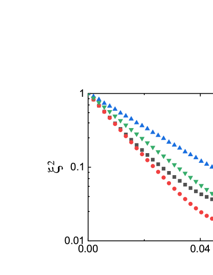
Figure 5: Numerical analysis of squeezing parameter of the LMG model (Black Square), TAT (Red Circle), the LMG model after pulse sequences along $y$-axis (Blue Triangle-Up), and the LMG model after pulse sequences along $z$-axis (Green Triangle-Down) with $N=100,\gamma=0.1$. For $0\leq\gamma\leq 0.5$, pulse sequences along the $z$-axis will have higher squeezing strength, thus leading to faster squeezing.

Figure 6: (a) Squeezing time of the $y$-pulse method (Blue Triangle-Up), and $z$-pulse method (Green Triangle-Down) with different $\gamma$. Insets: Effective squeezing strength of the $y$-pulse and $z$-pulse methods. (b) Squeezing ratio of the OAT, TAT, LMG, and pulse method.

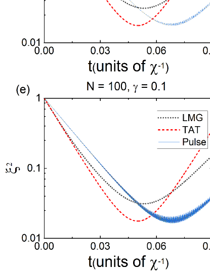
Figure 7: Numerical analysis of the influence of noises for our scheme with $N=100,\gamma=0.1$. The blue curves crowding together denote the results of 100 independent simulations under different noises. (a) Evolution of the squeezing parameter $\xi^{2}$ for 10% level of Gaussian stochastic noise adding on the pulse separation. (b) Evolution of the squeezing parameter $\xi^{2}$ for 0.02% level of Gaussian stochastic noise adding on the pulse area. (c) Evolution of the squeezing parameter $\xi^{2}$ for 0.01% level of Gaussian stochastic noise adding on $\gamma$. (d) Evolution of the squeezing parameter $\xi^{2}$ for 1% level of Gaussian stochastic noise adding on interaction strength $\chi$. (e) Evolution of the squeezing parameter $\xi^{2}$ for 0.01% level of Gaussian stochastic noise adding on atom number $N$. (f) Evolution of the squeezing parameter $\xi^{2}$ for 0.1% level of Gaussian stochastic noise adding on pulse stability.

For ${H_{\mathrm{LMG}}}=\chi({S_{x}^{2}+{\gamma}S_{y}^{2}})$, if we choose the $z$-axis to be the $\alpha$-axis, the time evolution operates for a single period is the following:

$${U_{z}} = e^{-i(S^{2}_{x}+\gamma S^{2}_{y})\chi t_{1}}R_{z,-\pi/2}e^{-i(S^{2}_{x}+\gamma S^{2}_{y})\chi t_{2}}R_{z,\pi/2}$$ (14)

$$= e^{-i(S^{2}_{x}+\gamma S^{2}_{y})\chi t_{1}}e^{-i(S^{2}_{y}+\gamma S^{2}_{x})\chi t_{2}.}$$

Using the Baker-Campbell-Hausdorff formula, we find $U_{z}\approx e^{-i\chi(S_{x}^{2}(t_{1}+\gamma t_{2})+S_{y}^{2}(\gamma t_{1}+t_{2}))}$ for small t. To transform the LMG model into TAT twisting, the coefficients should satisfy

$$\frac{t_{1}+\gamma t_{2}}{\gamma t_{1}+t_{2}}=0.5\text{ or }2.$$ (15)

Then the relationship between $\gamma$ and $t_{2}/t_{1}$ should satisfy

$$\frac{t_{2}}{t_{1}}=\frac{\gamma-2}{2\gamma-1}\text{ or }\frac{2\gamma-1}{\gamma-2}.$$ (16)

Accordingly, we obtain the effective Hamiltonian

$$H_{z}^{\mathrm{eff}} = \frac{\chi(\gamma+1)}{3}(S_{x}^{2}+2S_{y}^{2}),$$ (17)

$$\text{or }H_{z}^{\mathrm{eff}} = \frac{\chi(\gamma+1)}{3}(2S_{x}^{2}+S_{y}^{2}).$$ (18)

Similarly, if we choose the $y$-axis to be the $\alpha$-axis, we have the time evolution operator for a single period:

$${U_{y}} = e^{-i(S_{x}^{2}+\gamma S_{y}^{2})\chi t_{1}}R_{y,-\pi/2}e^{-i(S_{x}^{2}+\gamma S_{y}^{2})\chi t_{2}}R_{y,\pi/2}$$ (19)

$$= e^{-i(S_{x}^{2}+\gamma S_{y}^{2})\chi t_{1}}e^{-i(S_{z}^{2}+\gamma S_{y}^{2})\chi t_{2}}$$

To achieve TAT, we require $t_{2}/t_{1}=(\gamma+1)/(-\gamma+2)$ or $t_{1}/t_{2}=(\gamma+1)/(-\gamma+2)$. Then the resultant Hamiltonians read

$$H_{y}^{\mathrm{eff}} = \frac{\chi(1-2\gamma)}{3}(2S_{x}^{2}+S_{y}^{2}),$$ (20)

$$\text{or }H_{y}^{\mathrm{eff}} = \frac{\chi(2\gamma-1)}{3}(S_{x}^{2}+2S_{y}^{2}).$$ (21)

However, if we choose the $x$-axis to be the $\alpha$-axis, we will find that for $0\leq\gamma\leq 0.5$, $t_{1}/t_{2}\leq 0$, which means it’s impossible to transform the LMG model into TAT twisting making use of multi-pulse sequence along $x$-axis. The above pulse sequences are numerically verified with the results present in Fig. 5.

To make the squeezing occur faster, we need to shorten the squeezing time, which means getting higher squeezing strength $\chi^{\mathrm{eff}}$. As Fig. 6 (a) shows, for $0\leq\gamma\leq 0.5$, pulse along $z$-axis gets higher effective strength, which is $\chi^{\mathrm{eff}}_{z}=\chi(1+\gamma)/3$. And the squeezing time of the $z$-pulse method is also shorter compared with the $y$-axis pulse method.

Therefore, for a LMG model with arbitrary anisotropic parameter $\gamma$ ranging from 0 to 0.5, we can transform it into TAT interaction by using multi-pulse along different axes, and the squeezing performance of the LMG model after the pulse sequences will also reach Heisenberg scaling, as good as the TAT case, as compared in Fig. 6 (b).

Our scheme is robust to different kinds of noises. We carry out the numerical simulation by adding Gaussian stochastic noises, i.e., assuming the fluctuating pulse areas, pulse separations, pulse stability, $\gamma$, atoms number $N$, and interaction strength $\chi$, are subject to Gaussian distribution with a standard deviation of different ranges of the average value. The squeezing parameters of 100 independent simulations under different types of noises are respectively shown in Fig. 7. The numerical simulations show that our method is not only robust to internal systems noise such as uncertainty of determining $\gamma$, uncertainty of determining atoms number $N$, uncertainty of interaction strength $\chi$ but also external noise such as pulse areas noise, pulse separation noise, and pulse phase instability. Under certain kinds and ranges of noise, the best attainable squeezing of our method can almost achieve the optimal squeezing of the effective TAT dynamics.

As for the spin decoherence, our method itself will not bring new resources of decoherence but extend the squeezing time, while the coherence time for atoms such as Dysprosium is very long in spin squeezing [36], so we ignore the impact of extending evolution time for spin decoherence.

V Conclusion

In conclusion, we study the spin squeezing in systems with quadratic collective-spin interaction, which can be described by the LMG model. We find that the squeezing performance depends on the initial state and the anisotropic parameter. We show that the best initial state for $H=\chi(S^{2}_{x}+\gamma S^{2}_{y})$ is $\ket{\pi/2,\pi/2}$, which holds for different anisotropic parameter $\gamma$. We propose an implementable way with rotation pulses to transform the LMG model into TAT model with Heisenberg-limited spin squeezing. We find that pulse sequences applied along the $z$-axis will result in larger squeezing strength $\chi^{\mathrm{eff}}_{z}=\chi(1+\gamma)/3$ compared to the pulse sequences along the $y$-axis $\chi^{\mathrm{eff}}_{y}=\chi(1-2\gamma)/3$. Besides, our scheme is robust to noise in pulse areas and pulse separations. Our work will significantly increase the systems that could reach the Heisenberg scaling and will push the frontier of quantum metrology.

VI acknowledgement

We thank Prof. Fu-li Li for helpful discussions. This work is supported by the Key-Area Research and Development Program of Guangdong Province (Grant No. 2019B030330001), the National Natural Science Foundation of China (NSFC) (Grant Nos. 12275145, 92050110, 91736106, 11674390, and 91836302), and the National Key R&D Program of China (Grants No. 2018YFA0306504).

References

- [1] D. J. Wineland, J. J. Bollinger, W. M. Itano, F. L. Moore, and D. J. Heinzen, Phys. Rev. A 46, R6797 (1992).
- [2] M. Kitagawa and M. Ueda, Phys. Rev. A 47, 5138 (1993).
- [3] W. W. Ho and D. A. Abanin, Phys. Rev. B 95, 094302 (2017).
- [4] A. Sorensen, L.-M. Duan, J. I. Cirac, and P. Zoller, Nature 409, 63 (2001).
- [5] L. Amico, R. Fazio, A. Osterloh, and V. Vedral, Rev. Mod. Phys. 80, 517 (2008).
- [6] C. Orzel, A. K. Tuchman, M. L. Fenselau, M. Yasuda, and M. A. Kasevich, Science 291, 2386 (2001).
- [7] E. Pedrozo-Penafiel, S. Colombo, C. Shu, A. F. Adiyatullin, Z. Li, E. Mendez, B. Braverman, A. Kawasaki, D. Akamatsu, Y. Xiao, and V. Vuletic, Nature 588, 414 (2020).
- [8] R. Kaubruegger, P. Silvi, C. Kokail, R. van Bijnen, A. M. Rey, J. Ye, A. M. Kaufman, and P. Zoller, Phys. Rev. Lett. 123, 260505 (2019).
- [9] S. Colombo, E. Pedrozo-Penafiel, A. F. Adiyatullin, Z. Li, E. Mendez, C. Shu, and V. Vuletic, Nature Physics 18, 925 (2022).
- [10] J. G. Bohnet, B. C. Sawyer, J. W. Britton, M. L. Wall, A. M. Rey, M. Foss-Feig, and J. J. Bollinger, Science 352, 1297 (2016).
- [11] P. Cappellaro and M.D.Lukin, Phys.Rev.A.80.032311.
- [12] D. Farfurnik, Y. Horowicz, and N. Bar-Gill, Phys.Rev.A.98.033409
- [13] L.-G. Huang, F. Chen, X. Li, Y. Li, R. Lü, and Y.-C. Liu, npj Quantum Information 7, 168 (2021).
- [14] S. Zhou and L. Jiang, Phys. Rev. Research 2, 013235 (2020).
- [15] H. Zhou, J. Choi, S. Choi, R. Landig, A. M. Douglas, J. Isoya, F. Jelezko, S. Onoda, H. Sumiya, P. Cappellaro, H. S. Knowles, H. Park, and M. D. Lukin, Phys. Rev. X 10, 031003 (2020).
- [16] C. D. Marciniak, T. Feldker, I. Pogorelov, R. Kaubruegger, D. V. Vasilyev, R. van Bijnen, P. Schindler, P. Zoller, R. Blatt, and T. Monz, Nature 603, 604 (2022).
- [17] T. Ilias, D. Yang, S. F. Huelga, and M. B. Plenio, PRX Quantum 3, 010354 (2022).
- [18] M. A. C. Rossi, F. Albarelli, D. Tamascelli, and M. G. Genoni, Phys. Rev. Lett. 125, 200505 (2020).
- [19] Q. Liu, L.-N. Wu, J.-H. Cao, T.-W. Mao, X.-W. Li, S.- F. Guo, M. K. Tey, and L. You, Nature Physics 18, 167 (2022).
- [20] S.-F. Guo, F. Chen, Q. Liu, M. Xue, J.-J. Chen, J.-H. Cao, T.-W. Mao, M. K. Tey, and L. You, Phys. Rev. Lett. 126, 060401 (2021).
- [21] F. Yang, Y.-C. Liu, and L. You, Phys. Rev. Lett. 125, 143601 (2020).
- [22] S. P. Nolan, S. S. Szigeti, and S. A. Haine, Phys. Rev. Lett. 119, 193601 (2017).
- [23] C. L. Degen, F. Reinhard, and P. Cappellaro, Rev. Mod. Phys. 89, 035002 (2017).
- [24] W. Qin, Y.-H. Chen, X. Wang, A. Miranowicz, and F. Nori, Nanophotonics 9, 4853 (2020).
- [25] A. Kuzmich, L. Mandel, and N. P. Bigelow, Phys. Rev. Lett. 85, 1594 (2000).
- [26] Y. C. Liu, Z. F. Xu, G. R. Jin, and L. You, Phys.Rev. Lett. 107, 013601 (2011).
- [27] S. Dusuel and J. Vidal, Phys. Rev. B 71, 224420 (2005).
- [28] A. Glick, H. Lipkin, and N. Meshkov, Nuclear Physics 62, 211 (1965).
- [29] H. Lipkin, N. Meshkov, and A. Glick, Nuclear Physics 62, 188 (1965)
- [30] J. Vidal, G. Palacios, and C. Aslangul, Phys. Rev. A 70, 062304 (2004).
- [31] J. Ma and X. Wang, Phys. Rev. A 80, 012318 (2009).
- [32] T. E. Lee, F. Reiter, and N. Moiseyev, Phys. Rev. Lett. 113, 250401 (2014).
- [33] J. I. Cirac, M. Lewenstein, K. Molmer, and P. Zoller, Phys. Rev. A 57, 1208 (1998).
- [34] I. Carusotto and C. Ciuti, Rev. Mod. Phys. 85, 299 (2013).
- [35] Zeyang Li, Simone Colombo, Chi Shu, Gustavo Velez, Saúl Pilatowsky-Cameo, Roman Schmied, Soonwon Choi, Mikhail Lukin, Edwin Pedrozo-Peñafiel and Vladan Vuletić, arXiv:2212.13880 [quant-ph].
- [36] Thomas Chalopin, Chayma Bouazza, Alexandre Evrard, Vasiliy Makhalov, Davide Dreon, Jean Dalibard, Leonid A. Sidorenkov and Sylvain Nascimbene, Nat Commun 9, 4955 (2018).