Improving Survey Inference in Two-phase Designs Using Bayesian Machine Learning

Abstract

The two-phase sampling design is a cost-effective sampling strategy that has been widely used in public health research. The conventional approach in this design is to create subsample specific weights that adjust for probability of selection and response in the second phase. However, these weights can be highly variable which in turn results in unstable weighted analyses. Alternatively, we can use the rich data collected in the first phase of the study to improve the survey inference of the second phase sample. In this paper, we use a Bayesian tree-based multiple imputation (MI) approach for estimating population means using a two-phase survey design. We demonstrate how to incorporate complex survey design features, such as strata, clusters, and weights, into the imputation procedure. We use a simulation study to evaluate the performance of the tree-based MI approach in comparison to the alternative weighted analyses using the subsample weights. We find the tree-based MI method outperforms weighting methods with smaller bias, reduced root mean squared error, and narrower 95% confidence intervals that have closer to the nominal level coverage rate. We illustrate the application of the proposed method by estimating the prevalence of diabetes among the United States non-institutionalized adult population using the fasting blood glucose data collected only on a subsample of participants in the 2017-2018 National Health and Nutrition Examination Survey.

Keywords: Bayesian Additive Regression Trees (BART); High dimensional auxiliary variables; Multiple imputation; NHANES; Weighting.

1 Introduction

Over the past century, survey sampling has been applied to a wide range of scientific and industrial disciplines, such as healthcare, economomic policy, agriculture and environmental applications (Postelnicu et al., 1977; Hassan et al., 2020), for obtaining estimates of characteristics in the target population, e.g. disease prevalence and risk factors. Such estimates could provide useful information for decision-making and policy formulation (LaVange et al., 2001). However, if the desired measures are difficult or expensive to obtain, such as requiring sophisticated tests, it may not be feasible to collect these measures from all survey subjects given practical considerations and budget constraints. A two-phase sampling design can be used to overcome this challenge. The first phase selects a sample from a finite population using probability sampling, during which easy-to-access and inexpensive measures are collected (Hughes et al., 1996). The hard-to-obtain and expensive measures are then collected on a subsample selected from the phase-I sample. To give a better appreciation of the two-phase sampling, take the Mental Health Surveillance Study (MHSS) (Karg et al., 2014) as an example. The National Survey on Drug Use and Health (NSDUH) (Cotto et al., 2010) is a nationwide study that provides up-to-date information on tobacco, alcohol, and drug use, mental health and other health-related issues in the United States. MHSS used data from clinical interviews administered to a sub-sample of respondents of the NSDUH, aiming to make inferences of the prevalence of serious mental illness among people aged 18 years and older. Given that it is impractical to conduct clinical interviews with the entire NSDUH sample with approximately 46,000 adults participants, a phase-II subsample was selected to collect the serious mental illness data in the MHSS.

Statistical analysis of the phase-II sample could generate biased inference of population quantities if the distribution of the subsample is different from that of the population. A common approach for reducing bias in the subsample is weighting, which accounts for the subsample selection and nonresponse, and results in a new weight variable created by multiplying the weights for the Phase-I sample with the subsample weight adjustments (Kalton, 1986; Kalton and Miller, 1987). However, weighting has a number of limitations in two-phase designs. First, weighting adjustments can lead to highly variable weights for the Phase-II sample by multiplying the already variable weights for the phase-I sample with the additional weighting adjustments. Second, weights are less efficient in their use of phase-I participant data in that often only a subset of variables are used to reduce weight variability, and the adjustment focuses on differences between phase-I and phase-II samples and not the relationship with the outcome. Third, the weighting adjustments may produce biased estimates if the nonresponse propensity model used to create the phase-II weights is misspecified.

An alternative approach is to impute the outcome variables measured only in the Phase-II sample for the survey subjects who participate in Phase-I but not Phase-II of the study. This approach utilises the rich information collected for all participants in the Phase-I sample and a multiple imputation (MI) approach. After imputation, the population means are then estimated by applying the survey weights created for the Phase-I sample to the multiply-imputed phase-I data. Well-chosen imputation models can generate efficient estimates of population quantities (Kalton, 1986; Kalton and Miller, 1986; Chen et al., 2015). However, it can perform poorly if the imputation model is misspecified. Many works have been done to address the issue of model misspecification. Robins et al. (1994) proposed the augmented inverse propensity weighted (AIPW) estimator, which is a double robust (DR) estimator that can produce a consistent estimator if either the outcome model or propensity model is correctly specified. Penalized splines of propensity prediction (PSPP) is another DR estimator based on a Bayesian framework (Zhang and Little, 2009; Kim and Haziza, 2014). When both models are misspecified, however, these DR estimators fail to provide reliable estimates.

The risk of model misspecification motivates the use of non-parametric imputation models that are less sensitive to model misspecification. Bayesian Additive Regression Trees (BART), which was first proposed by Chipman et al. (2007), is a sum-of-trees machine learning model that has gained widespread popularity in recent years (Chipman et al., 2010). The essential idea of BART is to use the sum of multiple trees developed by Bayesian back-fitting Markov chain Monte Carlo (MCMC) to model the posterior distribution of the missing variables. BART allows the inclusion of a large number of predictors, rather than requiring the analyst to select a few. This method is less sensitive to model misspecification and allows for nonlinear effects and multi-way interactions between auxiliary variables and outcomes of interest. It was found that BART outperforms other machine learning methods (such as boosting, neural networks, and random forests) for prediction (Chipman et al., 2007). In addition to binary and continuous outcomes, BART has also been extended into different types of outcomes, such as count and categorical responses (Murray, 2021), semi-continuous outcomes (Linero et al., 2020), and survival outcomes (Sparapani et al., 2016).

BART and its extensions have been applied to a variety of research areas (Tan and Roy, 2019) including proteomic data (Hernández et al., 2015; Lualdi and Fasano, 2019), causal inference (Hill, 2011; Leonti et al., 2010; Hahn et al., 2020), missing data literature (Xu et al., 2016; Kapelner and Bleich, 2015) and survey inference (Liu et al., 2023; Rafei et al., 2022). Several advantageous features of BART were reported in the study of the cardiovascular proteomic high-dimensional data: 1) it can incorporate complex interactions between variables; 2) it can provide variable importance scores; 3) it had a higher AUC value compared with the Bayesian Lasso method (Hernández et al., 2015). BART was also applied to predict the counterfactual outcome when estimating the causal effect of historical texts on the frequency of medicinal plant use (Leonti et al., 2010). The benefits of BART for the propensity score adjustments have been demonstrated in the work of Kern et al. (2016) and Wendling et al. (2018). Given the superiority of BART, Tan et al. (2019) proposed extensions of the AIPW and PSPP that use BART to improve the robustness of doubly robust methods, and employed a simulation study to compare the performance of different methods. The results show that BARTps, which builds the outcome model with the additional estimated propensity by BART as predictors, performs better than other DR estimators when both models are misspecified. In addition, Liu et al. (2023) showed the efficiency of using BART and its extensions for estimating population means when high-dimensional auxiliary information is available in both the non-random samples and the target population. They demonstrate that BART and soft BART can yield efficient and accurate estimates of population means with coverage rates close to the nominal level. They also demonstrate that including the estimated propensity score as a predictor further improves inference when there is possible model-misspecification in the predictive model.

Inspired by and building on their work, we propose a tree-based MI approach to improve the inference of population means in two-phase designs. We apply BART and its extensions in two ways. Firstly we use BART-based models to adjust for difference between the phase-I and phase-II samples by creating subsample weights. Secondly we apply BART-based models to impute the phase-I sample for the variables only measured in the phase-II sample. We investigate the quality of population estimation by comparing these two approaches using a simulation study, with a real data illustration using the National Health and Nutrition Examination Survey (NHANES) data.

2 Motivating example: estimate prevalence of diabetes using NHANES data

Diabetes is one of the major causes of mortality. Patients with diabetes are more likely to have macrovascular and microvascular disease, increasing the health burden on their life. Over the past century, there has been an increase in the prevalence of diabetes (Harding et al., 2019; Ogurtsova et al., 2017; Wang et al., 2021). The increasing trend of diabetes and the profound effect it has on quality of life necessitates early diagnosis and intervention to prevent any complications (Yang et al., 2021). An accurate estimation of the prevalence of diabetes is also needed to provide a solid basis for policy-making about the prevention and management of diabetes.

NHANES is a series of cross-sectional, population-based surveys conducted by the National Center for Health Statistics to estimate disease prevalence, trends and the relationship between health and daily behaviour (Mishra et al., 2021). The procedure for collecting diabetes-related information in the NHANES is a two-phase sampling design. The phase-I sample is drawn from the target population of non-institutionalized United States residents through a four-stage stratified sample design. In the first stage, primary sampling units (PSUs) are selected with probability proportional to measures of size (PPS). The majority of these PSUs are single counties, but in a few cases, groups of contiguous counties. In the second stage, segments that include one or more contiguous census blocks are sampled among each selected PSU using PPS sampling. In the third stage, dwelling units (DUs) or households within each selected segment are randomly sampled at rates designed to produce a national, approximately equal probability sample. In the last stage, eligible individuals in each selected DU are invited to participate in the study. Individuals are randomly selected within designated age-sex-race/ethnicity screening groups.

In this application, we use the data of NHANES 2017-2018. Phase-I respondents are those belonging to the screened households who are selected and agree to participate in the interview and mobile examination. The basic demographic, health, and nutrition information for these phase-I respondents is collected through interviews and physical examinations in a mobile examination center. Individuals in the phase-I sample are randomly assigned to participate in three examination sessions (morning, afternoon, or evening). Physical examination results that require fasting, such as the fasting blood glucose (FBS) test, are collected only among individuals in the morning sessions, which we treat as the phase-II sample. From this subsample, we are interested in estimating the prevalence of diabetes among the non-institutionalised United States population aged 20 years or older. We define diabetes using two criteria: an FBS level higher than 126 mg/dL or HbA1c value higher than 6.5% according to the standard diagnosis method given by American Diabetes Association (American Diabetes Association, 2018). The FBS is only collected among the phase-II sample, but the HbA1c is measured in the phase-I study. Figure 1 shows the diagram of the two-phase sampling procedure for the FBS test data in NHANES.

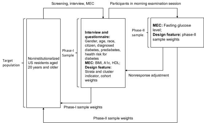
Figure 1: The two-phase sampling procedure for the fasting blood glucose test data in NHANES 2017-2018.

3 Methods

3.1 Notations and background

Let $\mathcal{P}$ represent a finite population of size $N$ with strata $h=1,\dots,H$, each of which has clusters $j=1,\dots,N_{h}$, where $N_{h}$ is the number of clusters for the $h$-th stratum. Let $y_{i}$ be the survey outcome of interest. The estimand of interest is the population mean $Q(y)=\sum_{i=1}^{N}y_{i}/N$. Let $\mathcal{C}$ denote the phase-I sample comprising of $n_{c}$ individuals selected from $\mathcal{P}$ using a stratified cluster sampling design; and $\mathbf{x}_{i}$ and $\mathbf{z}_{i}\in(0,1)$ are vectors of continuous and binary predictors for $i$-th individual with length $L_{1}$ (number of continuous predictors) and $L_{2}$ (number of binary predictors), respectively, which are collected at the individual level in the probability sample $\mathcal{C}$.

To make the sample $\mathcal{C}$ representative of the population $\mathcal{P}$, a first-phase weight, $w_{ci}$, is assigned to sample unit $i$ to adjust for unequal probability of selection and nonresponse, and calibrate to the population. When $y_{i}$ is fully observed for all the sample units in $\mathcal{C}$, the population mean can be estimated using

$$\hat{Q}_{c}(y)=\frac{\sum_{i=1}^{n_{c}}w_{ci}\cdot y_{i}}{\sum_{i=1}^{n}w_{ci}},$$ (1)

with variance estimated using the Taylor series linearization (Rust and Rao, 1996) or the resampling methods, such as jackknife repeated replicates, balanced repeated replicates, or bootstrap (Rao, 1996).

In the two-phase designs considered in this paper, however, $y_{i}$ is only measured among individuals who also participate in the second phase of the study, which is denoted by $\mathcal{S}$. Under this situation, Formula (1) cannot be applied directly. The conventional approach is to assign a subsample weight $w_{si}$ for the subsample in the second phase, which is often calculated as the product of the sample weight $w_{ci}$ and an adjustment reflecting the potential unequal probability of selection and nonresponse for the subsample units. The selection probability can be easily calculated based on the sampling procedure. The nonresponse adjustment can be obtained using either an adjustment cell method or a propensity score adjustment method. In our simulations we use BART to create a propensity score adjustment and compare it to a tree-based adjustment cell method. The population mean using the subsample is estimated as

$$\hat{Q}_{\mathcal{S}}(y)=\frac{\sum_{i=1}^{n_{s}}w_{si}\cdot y_{i}}{\sum_{i=1}^{m}w_{si}}$$ (2)

where $n_{s}$ is the sample size of the subsample.

For the subsample nonresponse adjustment, the adjustment cell approach assigns units in the sample into different cells $m=1,\dots,M$ with size $n_{m}$ based on discretized auxiliary information $\mathbf{x}$ and binary $\mathbf{z}$. The response status indicator for $i$-th unit is denoted by $r_{i}$, with $r_{i}=1$ for respondents, $r_{i}=0$ for non-respondents. The estimated response rate in the $m$-th cell is $\hat{\pi}_{m}=\sum_{i=1}^{n_{m}}r_{i}/n_{m}$, and the nonresponse adjustment for all units in the $m$-th cell is $1/\hat{\pi}_{m}$. It assumes that respondents and nonrespondents in the same cell have the same distributions in the survey outcomes of interest (Little and Vartivarian, 2005; Kalton and Flores-Cervantes, 2003). However, this method requires that all continuous variables $\mathbf{x}$ are discretized, and as the number of auxiliary variables grows large, the cell size and the number of response units in a specific cell decreases quickly, resulting in extreme and nonstable weighting adjustments (Kalton and Flores-Cervantes, 2003).

One solution for this is tree-based methods. The chi-square automatic interaction detection (CHAID) (Kass, 1980) is commonly used for nonresponse adjustment in survey sampling. It selects important auxiliary variables and forms adjustment cells through a merge-and-split process (Kass, 1980). For each variable, a chi-square test is conducted to test the independence between two different categories of a variable. If the chi-square test fails to reject the null with a user-specified alpha-level, these categories are merged into a single category. These merging steps are repeated until all of the categories are significantly different for each predictor. When splitting, the predictor with the smallest Bonferroni-adjusted p-value is chosen as the first split, and the splitting continues until: a) no significant predictors; b) the child node will have insufficient individuals if more splits are made; c) the number of individuals in some nodes is below a pre-specified number (Chen et al., 2015).

Another method to adjust for nonresponse is propensity score adjustment. Logistic regression is commonly used to estimate the response propensity(Rizzo et al., 1996):

$$\text{logit}(Pr(r_{i}=1|\mathbf{x}_{i},\mathbf{z}_{i}))=\gamma_{0}+\mathbf{\gamma}_{1}^{T}\mathbf{x_{i}}+\mathbf{\gamma}_{2}^{T}\mathbf{z_{i}}$$ (3)

where $\mathbf{\gamma}_{1}$ and $\mathbf{\gamma}_{2}$ are vectors of coefficients for $\mathbf{x}_{i}$ and $\mathbf{z}_{i}$. Screening of response-related variables is often conducted before building the propensity model (Rizzo et al., 1996). In contrast to the adjustment cell methods, it allows both discrete and continuous variables to be used as predictors of response propensity. Propensity score adjustment can be divided into two categories. The first is response propensity weighting where the nonresponse adjustment is the inverse of the probability of responding. However, it has some limitations: the first is that it can generate very small response propensities and thus very large weighting adjustments leading to unstable estimation of population quantities; Secondly, it relies on the correct specification for the response propensity model. The estimates for subsample weights will be biased if the response propensity model is misspecified.

3.2 Imputation methods using Bayesian Additive Regression Trees

Instead of viewing this challenge as an adjustment from the subsample to the finite population, we could instead consider this first as a missing data problem in the phase-I sample and then survey inference of population quantities using the imputed phase-I sample. Weights-based analyses use auxiliary variables in the phase-I sample to calculate nonresponse adjustments in the subsample. This wastes important information about the relationship between these variables and the outcome we wish to estimate. In contrast, an imputation approach can best use the associations between the auxiliary information and the outcome.

BART (and related extensions) are sum-of-tree Bayesian models that are flexible in model specification and can achieve high accuracy of prediction by incorporating interactions and nonlinear associations without overfitting (Tan and Roy, 2019). Liu et al. (2023) proposed using BART and soft BART to improve the robustness of the estimators of population means in one-phase survey sampling. They showed that an outcome model built by BART or soft BART can generate efficient estimates of population means by using the rich auxiliary data information available in both the population and the survey sample and the BART-estimated inclusion propensity scores as predictors. In this paper, we extend this idea to two-phase complex survey designs.

We consider the following BART model for continuous survey outcomes measured only in the subsample of the Phase-II study:

$$y_{i}=G(\mathbf{x}_{i},\mathbf{z}_{i},d_{i1},d_{i2},\mathbf{w}_{i})+\epsilon_{i}=\sum_{b=1}^{B}g\left(\mathbf{x}_{i},\mathbf{z}_{i},d_{i1},d_{i2},\mathbf{w}_{i};T_{b},\mathbf{\mu}_{b}\right)+\epsilon_{i},\quad\epsilon_{i}\ \sim N(0,\sigma^{2}),$$ (4)

where $d_{i1}$ and $d_{i2}$ denote strata and cluster indicators for $i$-th individual respectively; $\mathbf{w}_{i}$ represents survey weights, including phase-I sample weights $w_{ci}$ and subsample selection and nonresponse weighting adjustments $a_{i}$; $B$ is the number of trees, $T_{b}$ is the structure of b-th binary tree, $\mu_{b}$ is the parameters assigned to each terminal node, and $g(\cdot)$ is the function that links $\mu_{b}$ to ($\mathbf{x}_{i}$, $\mathbf{z}_{i}$, $d_{i1}$, $d_{i2}$, $\mathbf{w}_{i}$).

One challenge for BART is the prior specification. Chipman et al. (2010) simplified the prior specification by assuming that the components of each tree are independent and not related to the error term $\epsilon$. Under this assumption, the priors for $p(T_{b})$, $p(\mu_{b}|T_{b})$, and $p(\sigma^{2})$ need to ensure that every tree is a weak learner and prevent the model from overfitting and non-convergence. The prior for $p(T_{b})$ is related with: i) the probability of being nonterminal for a node at depth $\rho=0,1,2,\dots$, which is specified by $\alpha(1+\rho)^{-\beta}$, where $\alpha\in(0,1)$, $\beta\in[0,\infty)$; ii) the probability of being selected as a splitting variable; iii) for the selected splitting variable, the probability of splitting rules. A conjugate normal distribution is used for the prior of $p(\mu_{b}|T_{b})$. For $p(\sigma^{2})$, an inverse chi-square distribution is used such that $\sigma^{2}\sim\nu\lambda/\chi_{\nu}^{2}$. Chipman et al. (2010) suggest default values for the parameters of these prior distributions and the number of trees B, but cross-validation can be used to select the optimal parameters for these priors.

To account for the correlation between units from the same cluster in the first-phase sampling, we also consider random intercept BART (rBART) (Tan et al., 2018), which is an extension of BART. The outcome model by rBART is then

$$y_{ji}=G(\mathbf{x}_{ji},\mathbf{z}_{ji},d_{ji1},\mathbf{w}_{ji})+\delta_{j}+\epsilon_{ji}=\sum_{b=1}^{B}g(\mathbf{x}_{ji},\mathbf{z}_{ji},d_{ji1},\mathbf{w}_{ji};T_{b},\mu_{b})+\delta_{j}+\epsilon_{ji},\quad\epsilon_{ji}\sim N(0,\sigma^{2}),$$ (5)

where $\delta_{j}$ is the random intercept for $j$-th cluster which follows a normal distribution and independent of the individual error term $\epsilon_{ji}$. Each cluster is seen as a group with the same random intercept in the stratified survey design. For a binary outcome, BART and rBART can be easily extended by the probit model:

$$Pr(y_{i}=1|\mathbf{x}_{i},\mathbf{z}_{i},d_{i1},d_{i2},\mathbf{w}_{i})=\Phi(G(\mathbf{x}_{i},\mathbf{z}_{i},d_{i1},d_{i2},\mathbf{w}_{i}))$$ (6)

where $\Phi$ is the cumulative density function of a standard normal distribution.

In a two-phase complex survey setting, the data in the subsample are used to build the BART imputation model, and the unobserved outcome variable for subjects who participate in the Phase-I survey but not the Phase-II survey is then imputed using posterior draws from the model. Before building the imputation model for the outcome, BART and rBART can also be used to estimate the nonresponse adjustment, $a_{i}$ with $x_{i}$, $z_{i}$, $w_{ci}$, $d_{i1}$ and $d_{i2}$ as predictors. The imputation model is then fit with the estimated $a_{i}$ included in the list of predictors. For BART, both $d_{i1}$ and $d_{i2}$ are categorical predictors. However, in rBART, $d_{i2}$ is used as a group indicator. Each set of posterior draws forms one imputation for the missing $y$ in the phase-I sample. Let $\hat{y}_{i}^{d}$ denote the imputed value of $y$ for individual $i$ in the $d$th imputation of the Phase-I sample, $d=1,\dots,D$ and $D$ is the total number of imputations. We have $\hat{y}_{i}^{(d)}=I(i\in\mathcal{S})y_{i}+I(i\in\mathcal{C},\ i\notin\mathcal{S}){\hat{y}}_{i}^{d}$. The estimated population mean using the $d$th imputation is calculated as

$$\hat{Q}(y)^{(d)}=\frac{\sum_{i=1}^{n_{c}}w_{ci}\cdot{\hat{y}}_{i}^{(d)}}{\sum_{i=1}^{n_{c}}w_{ci}},$$ (7)

with the estimated variance $\widehat{Var}\left(\hat{Q}(y)^{(d)}\right)$ by the Taylor series linearization method to account for the sampling design and non-response (Rust and Rao, 1996).

The estimates in (7) are then combined from the $D$ imputations using the Rubin’s multiple imputation rules with the variance accounting for both between-imputation and within-imputation variances (Little and Rubin, 2002):

$$\hat{Q}(y)=\frac{1}{D}\sum_{d=1}^{D}\hat{Q}(y)^{(s)},~{}~{}~{}\widehat{Var}\left(\hat{Q}(y)\right)=\bar{W}_{D}+(1+\frac{1}{D})B_{D},$$ (8)

where $\bar{W}_{D}=\frac{1}{D}\sum_{d=1}^{D}\widehat{Var}\left(\hat{Q}(y)^{(d)}\right)$ and $B_{D}=\frac{1}{D-1}\sum_{d=1}^{D}(\hat{Q}(y)^{(d)}-\hat{Q}(y))^{2}$ are the estimated within and between imputation variance, respectively. The reference distribution for confidence interval estimates is a $t$ distribution,

$$\frac{Q(y)-\hat{Q}(y)}{\sqrt{\widehat{Var}\left(\hat{Q}(y)\right)}}\sim t_{\nu},$$ (9)

with the degrees of freedom based on a Satterthwaite approximation,

$$\nu=(D-1)(1+\frac{D}{D+1}\frac{\bar{W}_{D}}{B_{D}})^{2}.$$ (10)

Based on Liu et al. (2023), three assumptions should hold for the MI approach using BART to perform well in the two-phase designs: (A1) outcome-related auxiliary variables are available in the phase-I sample; (A2) the sampling mechanism and response propensity in the subsample is conditionally ignorable, i.e., the outcome variable $y$ is independent of subsample selection and the response given the auxiliary information and design features in the Phase-I sample; and (A3) the auxiliary variables in the subsample and in the phase-I sample have the same ranges. Assumption A3 fails in cases where the sampling mechanism or response propensity makes the ranges of the auxiliary variables in the phase-I sample wider than those in the subsample (e.g., if individuals in a particular range of the predictor $x$ are never included in the subsample).

4 Simulation

We conduct a simulation study to evaluate the performance of weighting and tree-based MI approaches in a two-phase survey design. We compare 4 different weighting methods for the nonresponse adjustments, including logistic regression model (LGM), CHAID, BART and rBART, with the corresponding estimators denoted using WT-LGM, WT-CHAID, WT-BART and WT-rBART. We also consider the MI approach using 2 tree-based models (MI-BART and MI-rBART). For reference, we include a benchmark estimator, where the outcome $y$ is assumed to be measured for all subjects in the phase-I sample. We conduct 500 replicates of simulation for each simulation scenario. Model performance is evaluated by the absolute bias and root mean squared error (RMSE),

$$\textrm{Absolute bias}=\left|{\frac{\sum_{s=1}^{500}(\hat{Q}(y)^{(s)}-Q(y))}{500}}\right|,~{}~{}\textrm{RMSE}=\sqrt{\frac{\sum_{s=1}^{500}(\hat{Q}(y)^{(s)}-Q(y))^{2}}{500}},$$

where $s=1,\dots,500$ is the $s$-th simulation replicate. We also investigate the coverage rate and average width of the 95% CIs. These measurements are magnified a hundred times for the convenience of reading.

4.1 Sampling design

This subsection gives detailed steps to generate two-phase multistage complex survey data. Our process is inspired by the simulation design in Liu et al. (2023).

1. Population: We first generate finite population $\mathcal{P}$ with 4 strata ($H=1,2,3,4$), each of which has $N_{h}=25,20,15,10$ clusters respectively. The number of individuals in each cluster, $N_{hj}$, follows an exponential distribution truncated between 100 and 300, with expected values as 200. This leads to a population of size $N=12,931$. For each individual in the population, we generate data for continuous variables $x_{l_{1}}$, $l_{1}=1,\dots,L_{1}$, and binary variables $z_{l_{2}}$, $l_{2}=1,\dots,L_{2}$. The continuous variables $x_{l_{1}}$ follows a standard normal distribution $N(0,1)$. For each binary variable, $Pr(z_{l_{2}}=1)$ follows a uniform distribution $U\left(0.4,0.6\right)$.

2. Outcome model: We consider a continuous outcome variable for the $i$th subject in the $j$th cluster of the $h$th stratum by specifying the true outcome model as

   $$y_{hji}=2.47+q_{hj}-2x_{1hji}+x^{2}_{2hji}+2z_{1hji}-z_{2hji}-2z_{3hji}+x_{1hji}z_{1hji}+\epsilon_{hji},~{}\epsilon_{hji}\sim N(0,1)$$

   where $q_{hj}$ is the cluster random intercept which follows a normal distribution $N(0,1)$. The true population mean of the outcome is $Q(y)=3$.

3. Phase-I sample: To select the phase-I sample, we draw $n_{h}=10,8,6,4$ clusters respectively from each stratum $h=1,2,3,4$ using PPS sampling with size equal to the number of units in each cluster (Rosén, 1997), i.e., the selection probability for each cluster is proportional to its cluster size and equals to $\frac{n_{h}N_{hj}}{\sum_{j}^{N_{h}}N_{hj}}$. The base weight $w_{0hj}$ can be calculated as the inverse of the selection probability $w_{0hj}=\frac{\sum_{j}^{N_{h}}N_{hj}}{n_{h}N_{hj}}$. All the units in the selected clusters are invited to participate in the study but not all respond. The response probability for $i$th subject in the $j$th selected cluster of the $h$th stratum is calculated as:

   $$\pi_{hji,res,1}=\textrm{logit}^{-1}(-1+2z_{1hji}+2z_{2hji}-z_{3hji}).$$ (11)

   This sampling procedure results in a phase-I sample with approximately $3,000$ individuals.

4. Phase-II sample: To collect outcome data, we select a subset of phase-I sample by simple random sampling with a selection probability of 0.5. Given that there may be some nonrespondents among the selected individuals for the phase-II sample, we consider four scenarios for the response patterns:

   1. Low dimensional auxiliary variables ($L_{1}=2$, $L_{2}=3$) collected in the phase-I sample. The true response propensity model is

      $$\pi_{hji,res,2}=\textrm{logit}^{-1}(1+2x_{hji1}+1.5x_{hji2}^{2}+2z_{hji1}+z_{hji2}-2z_{hji3}-x_{hji1}z_{hji1}).$$

      Units in the lower tail of $x_{hji1}$ and $x_{hji2}$ have lower probability of response in the Phase-II sample.

   2. High dimensional auxiliary variables ($L_{1}=10$, $L_{2}=10$) collected in the phase-I sample. The true response propensity model is the same as S1, with the only difference that there are many noise variables $x_{3},\dots,x_{10}$, $z_{4},\dots,z_{10}$ that are not associated with outcome $Y$ and response propensity collected in the phase-I sample.

   3. High dimensional auxiliary variables ($L_{1}=10$, $L_{2}=10$) collected in the phase-I sample with the assumption A3 violated in the outcome-related variables. The true response propensity model is specified as

      $$\pi_{hji,res,2}=\textrm{logit}^{-1}(1+2x_{hji1}-1.5x_{hji2}^{2}+2z_{hji1}+z_{hji2}-2z_{hji3}-x_{hji1}z_{hji1}).$$

      The only difference between S3 and S2 is that the sign of the coefficient for $x_{hji2}^{2}$ is changed to negative values such that there are sparse data in the higher and lower tails of $x_{hji2}$.

   4. High dimensional auxiliary variables ($L_{1}=10$, $L_{2}=10$) collected in the phase-I sample with the assumption A3 violated in the variables that are not related with outcome. The true response propensity model is specified as

      $$\pi_{hji,res,2} =\textrm{logit}^{-1}(1+2x_{hji1}-1.5x_{hji3}^{2}+2z_{hji1}+z_{hji2}-2z_{hji3}-x_{hji1}z_{hji1}).$$

      In this scenario, the higher and lower tails of $x_{hji3}$ is under-sampled, and the ranges of $x_{hji3}$ in the phase-II sample and phase-I sample are different, but $x_{hji3}$ is not related to $y_{hji}$.

Note that for all the scenarios mentioned above, the LGM for the prediction of response propensity does not include nonlinear or interaction terms, so WT-LGM is faced with the issue of model misspecification. We specify the number of trees as $B=100$ and use the default prior specification in BART and rBART in the simulation and motivating examples.

Figure 2 shows scatter plots of Phase-I and Phase-II samples in a simulation for scenarios S1-S4. The y-axis is the outcome $y$, and the x-axis is the continuous variable $x_{2}$ that is associated with $y$. The light grey dots represent the phase-I units that are not in the phase-II sample; dark grey triangles denote the phase-I units that are in the phase-II sample. In scenario S1, S2 and S4 (Figure 2A, Figure 2B, and Figure 2D respectively), the range of $x_{2}$ are the same in phase-I and phase-II samples; however, in scenario S3, the phase-I units in the higher and lower tails of $x_{2}$ are less likely to respond in the phase-II.

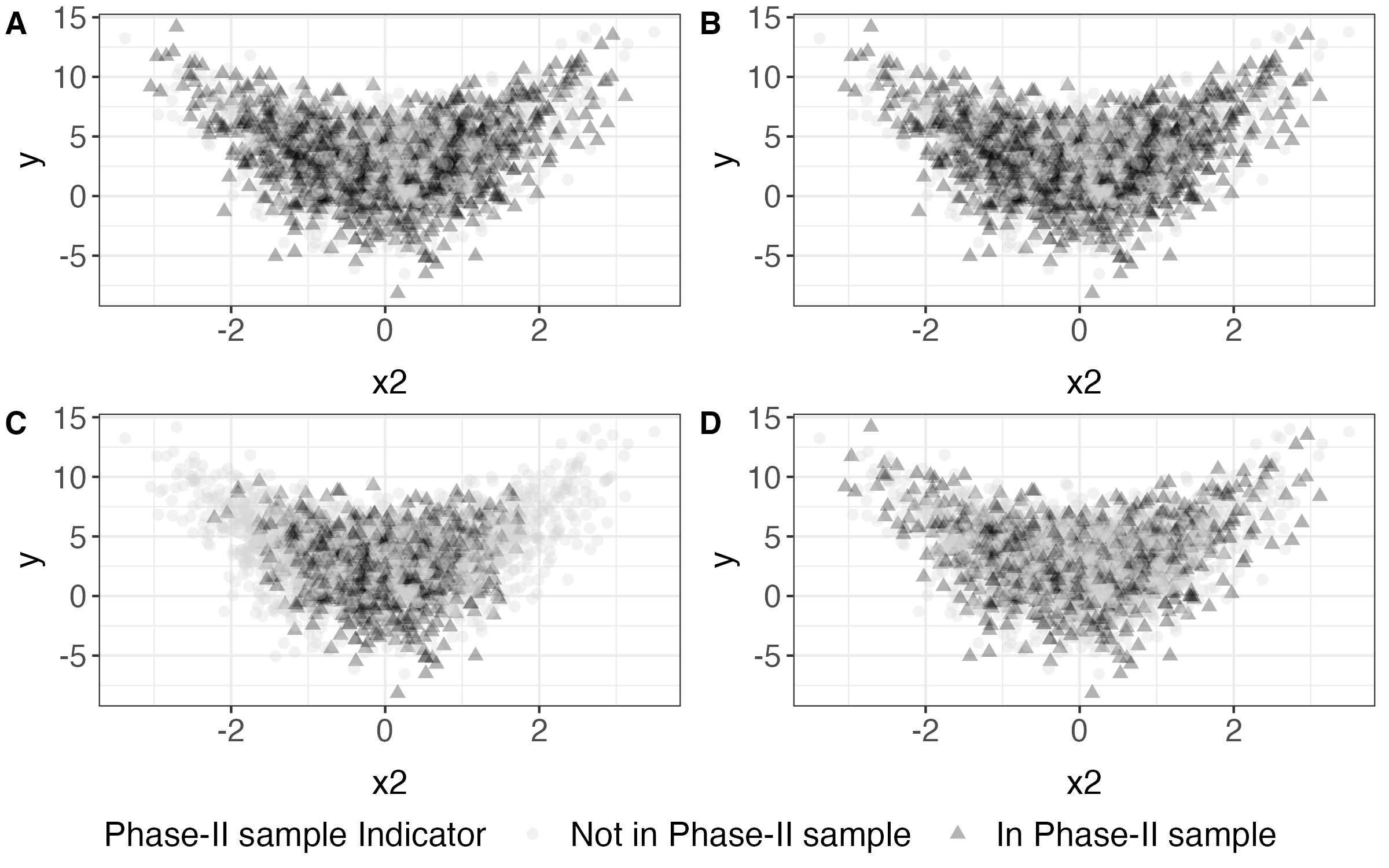
Figure 2: Scatter plots of outcome $y$ against continuous variables $x_{2}$. Light grey dots represent subjects in the phase-I sample but not in the phase-II sample; Dark grey triangles represent subjects in the phase-I sample and also in the phase-II sample. A, B, C, and D correspond to simulation scenarios S1, S2, S3, and S4, respectively.

Scenarios S2-S4 are designed to compare the performance of the competing methods in real-world settings where massive auxiliary information is available in the Phase-I sample, and researchers have no clear thoughts about the truly important predictors for the response propensity or the desired outcome. Under these three scenarios, for implementing the WT-LGM and WT-CHAID methods, we first use Lasso (Tibshirani, 1996) to select “important” variables for the response propensity before fitting a LGM or CHAID model. Scenarios S3 and S4 are set up to investigate the impact of violation of assumption A3 mentioned in Section 3.2 on the model performance.

4.2 Simulation results

Figure 3 shows the simulation results using $D=10$ imputations, where the y-axis is the value of each metric. The simulation results using $D=20,50,100,500,1000$ are presented in eFigure 1-5 in the supplementary materials. As we expect, the benchmark estimator performs the best, with the lowest absolute bias and RMSE, shortest interval width, and close to the nominal level coverage rate. The MI-based estimators yield similar bias and RMSE with the benchmark estimator under Scenarios S1 and S2 but larger bias and RMSE under Scenarios S3 and S4. Compared to the weighting-based methods, the MI-based methods have lower bias and RMSE in all scenarios, with comparatively smaller interval width, especially when compared with the weighting methods using LGM and CHAID. The coverage rate of the 95% CI for both the MI-based estimators are close to the nominal level in all scenarios.

In scenario S3 (3rd axis tick), when the assumption A3 is violated by the sparse data in the tails of outcome-related variable $x_{2}$, both the imputation and weighting methods perform worse than the other scenarios, especially for the LGM weighting methods with largest bias and RMSE. It’s not surprising given that the models cannot well assess the relationship between the outcome and the covariates and between response propensity and the covariates outside the range of $x_{2}$ in the sample. However, the MI-based methods still perform better than the weighting methods under this condition with a much smaller bias and RMSE. For scenario S4 with assumption A3 violated due to the sparse data in the tails of $x_{3}$, a variable not correlated with $y$, the performance of the tree-based imputation methods is still promising, with slightly wider confidence intervals and larger RMSE than in scenarios S1 and S2, but still better performance than the BART and rBART weighting based methods.

For weighting-based methods, the bias and RMSE for the estimators using BART/rBART models to estimate response propensity is slightly larger than the corresponding MI-based estimators in scenarios S1 and S2. However, they are all smaller than those using LGM or CHAID to estimate response propensity. The interval widths are also smaller for BART/rBART-based weighting methods compared with LGM in scenarios S1 and S2. For scenarios S3 and S4, the interval widths for BART/rBART-based weighting methods are wider than the other methods. The WT-LGM has the largest absolute bias because the model for nonresponse adjustments ignores possible interactions and nonlinear associations.

When comparing between BART and rBART-based imputation methods, rBART has a slightly smaller bias than BART, with the biggest improvement observed for Scenarios S3. Also, MI-rBART has wider interval width than MI-BART. This may be explained by the additional random intercept term in the rBART model. When we increase the number of imputations from $10$ to $1000$, the simulation results are almost unchanged. This suggests 10 imputations are sufficient for the MI-BART and MI-rBART methods.

Overall, the MI-based estimators perform better than the weighting methods, generating less biased and more efficient estimates of population quantities, with shorter interval widths at no expense of coverage rate. By using BART/rBART-based MI methods, we can accurately estimate the relationship between auxiliary variables and $y$ in the high-dimensional covariates setting with non-linear associations and interactions, and thus best use the rich data information collected in the Phase-I sample to improve the estimation of population quantities using the Phase-II sample. The assumption A3 is critical, especially for the covariates associated with $y$. When conducting weighting analysis, BART-based models can be an attractive alternative to the linear logistic regression and the CHAID models.

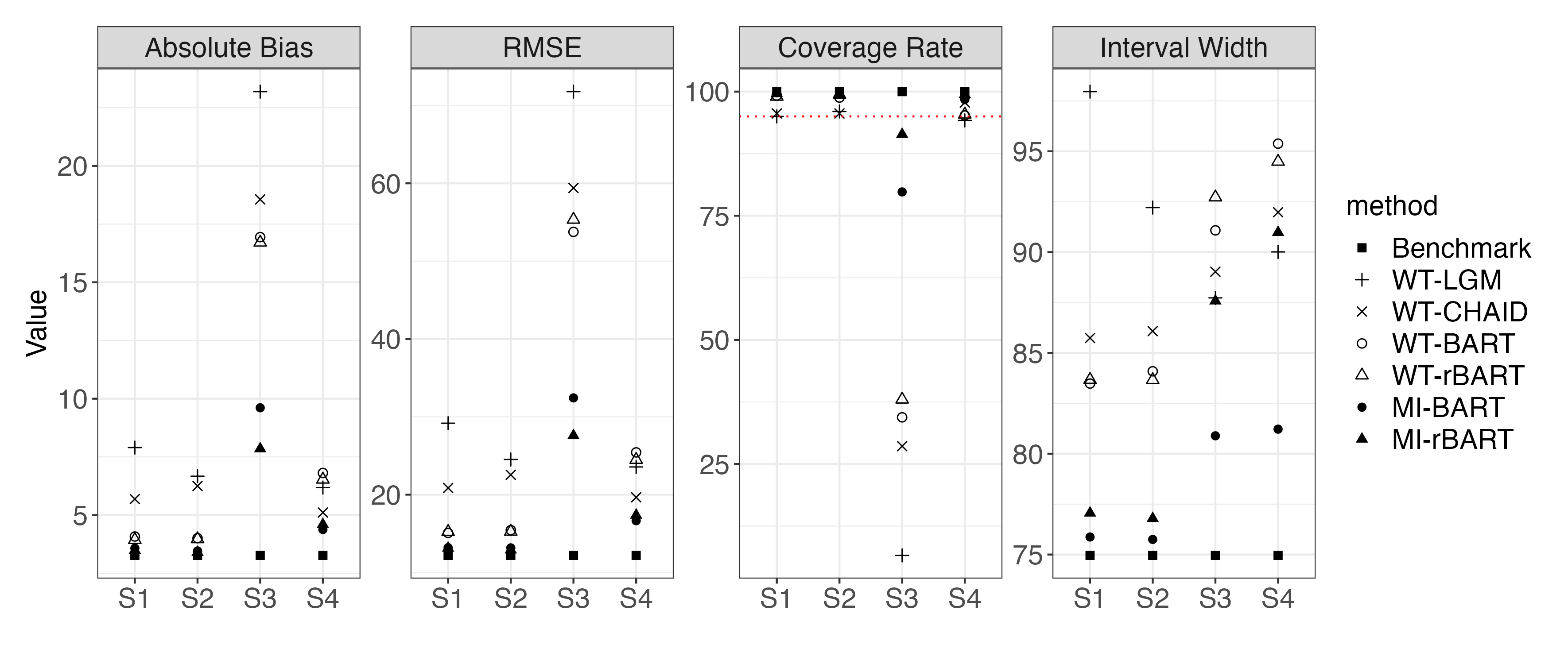
Figure 3: Simulation results with the number of imputations $D=10$. WT-LGM, WT-CHAID, WT-BART and WT-rBART are weighted analysis based on the Phase-II sample and using the Phase-II sample weights, MI-BART, and MI-rBART are the tree-based imputation methods. S1: low dimensional case where all the assumptions holds; S2: high dimensional case where all the assumptions holds; S3: high dimensional case where assumption (A3) does not hold for a outcome-related variable; S4: high dimensional case where assumption (A3) does not hold for a variable not related with the outcome.

5 The National Health and Nutrition Examination Survey

We illustrate the application of the proposed tree-based imputation method using the NHANES 2017-2018 data. The goal is to estimate the prevalence of diabetes among the United States non-institutionalised adult population, defined as an individual with a fasting blood sugar (FBS) level higher than 126 mg/dL or HbA1c value higher than 6.5% (Ghazanfari et al., 2010; Emancipator, 1999). Our phase-I sample are the $5,265$ NHANES 2017-2018 participants who completed the interviews and the MEC examination. All participants in the MEC examination had their HbA1c measured. The MEC examination weights are provided by NHANES to account for unequal probability of selection and unit nonresponse during interviews and examinations. Of these, only participants in the morning sessions are eligible for a FBS test (which requires an 8-hour fast). The $2,295$ participants who participated in the morning sessions are our phase-II sample. The subsample weights are also available in the NHANES data.

The descriptive statistics of the covariates that are measured in the Phase-I sample and included in the BART/rBART models are summarized in Table 1. These variables include demographic information (age, gender, race, citizen), physical examination results (BMI, HbA1c, HDL), and diabetes-related self-reported data (diagnosed diabetes - ever told by doctors that you had diabetes, DIQ160 - ever told had prediabetes, DIQ170 - ever told had health risk for diabetes, DIQ172: feel could be at risk for diabetes, BPQ020: ever told had high blood pressure, ALQ151: ever had 4/5 or more drinks every day, SMQ040: whether smoke cigarettes). The distributions of these variables between the phase-I and phase-II samples are similar. There are small proportions of missing data in some of these variables. We use the Chained Equations imputation algorithm, implemented in the “mice” package in R, to fill in the missing data in these covariates.

Table 1: Descriptive statistics analysis of NHANES 2017-2018 data.

Characteristics	Phase-I sample	Phase-II sample
	(N = 5,265)	(N = 2,295)
Gender
Male	2,541 (48%)	1,096 (48%)
Female	2,724 (52%)	1,199 (52%)
Age
20-39	1,589 (30%)	688 (30%)
40-59	1,658 (31%)	742 (32%)
60+	2,018 (38%)	865 (38%)
Race
Mexican American	698 (13%)	336 (15%)
Other Hispanic	496 (9.4%)	218 (9.5%)
Non-Hispanic White	1,807 (34%)	764 (33%)
Non-Hispanic Black	1,240 (24%)	519 (23%)
Non-Hispanic Asian	759 (14%)	329 (14%)
Other Race	265 (5.0%)	129 (5.6%)
Citizen
Citizen by birth	4,516 (86%)	1,966 (86%)
Not a citizen of the US	727 (14%)	320 (14%)
Missing	22 (0.4%)	9 (0.4%)
BMI (kg/m*2)	30 (25, 34)	30 (25, 34)
HbA1c (%)	5.87 (5.30, 6.00)	5.88 (5.30, 6.00)
Direct HDL-Cholesterol (mmol/L)	1.38 (1.09, 1.60)	1.38 (1.09, 1.58)
DIQ160*
No	3,709 (70%)	1,585 (69%)
Yes	551 (10%)	240 (10%)
Missing	1,005 (19%)	470 (20%)
DIQ170*
No	3,648 (69%)	1,566 (68%)
Yes	768 (15%)	333 (15%)
Missing	849 (16%)	396 (17%)
DIQ172*
No	3,018 (57%)	1,293 (56%)
Yes	1,351 (26%)	581 (25%)
Missing	896 (17%)	421 (18%)
BPQ020*
No	3,243 (62%)	1,413 (62%)
Yes	2,012 (38%)	878 (38%)
Missing	10 (0.2%)	4 (0.2%)
ALQ151*
No	3,688 (70%)	1,644 (72%)
Yes	679 (13%)	304 (13%)
Missing	898 (17%)	347 (15%)
SMQ040*
Every day	755 (14%)	316 (14%)
Some days	203 (3.9%)	85 (3.7%)
Not at all	1,251 (24%)	562 (24%)
Missing	3,056 (58%)	1,332 (58%)
diagnosed_diabetes*	836 (16%)	390 (17%)
1 n (%); Mean (IQR)
2 DIQ160: Ever told you have prediabetes; DIQ170: Ever told have health risk for diabetes;
DIQ172: Feel could be at risk for diabetes; Diagnosed diabetes: Doctor told you have diabetes;
BPQ020: Ever told had high blood pressure; ALQ151: Ever have 4/5 or more drinks every day?
SMQ040: Do you now smoke cigarettes?

To infer the population prevalence of diabetes, we compare the traditional weighting method using the phase-II sample weights provided by NHANES to tree-based imputation methods using BART and rBART. As the FBS level data are only available in the phase-II sample, for tree-based imputation methods, we first impute the FBS level data in the phase-I sample, and then use the imputed FBS and the observed HbA1c to define the presence of diabetes among participants in the Phase-I sample. We finally conduct weighting analysis from the multiply imputed phase-I sample using the Phase-I sample weights provided by NHANES. To impute the FBS level in the Phase-I sample, the auxiliary variables in Table 1, stratum and cluster indicators, and phase-I sample weights are included in the imputation models. Before fitting the imputation models, we examine assumption A3 by exploring the distributions of the continuous auxiliary variables in the Phase-I and Phase-II samples. Figure 6 in the supplementary materials shows that ranges of BMI, HbA1c, and HDL in the phase-I sample are similar to those in the phase-II sample. We also pre-processed the data in NHANES by log-transforming BMI, HbA1c, HDL, and the phase-I weights. For rBART, we included cluster indicators as group indicators in the model. For each imputation-based estimator, 10 imputations of the FBS variable are generated.

As is shown in Figure 4, the estimate for the prevalence of diabetes using BART and rBART imputation methods are 14.3% (95% CI: 13.0%, 15.5%) and 14.2% (95% CI: 12.9%, 15.4%) respectively, which are slightly higher than using the NHANES weights for the phase-II sample (13.7%, 95% CI: 11.8%, 15.8%). The weighted estimate using the NHANES weights for the Phase-II sample also yields a wider 95% CI than the imputation-based estimates.

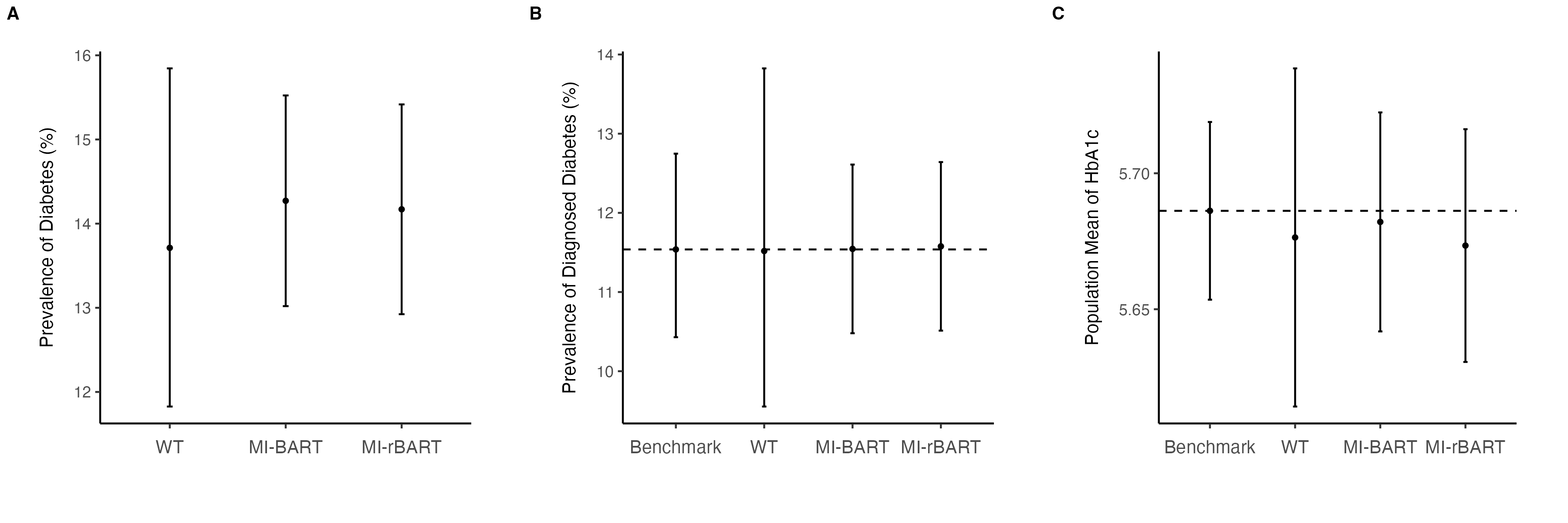
Figure 4: Application results. A: point estimates and 95% confidence intervals for the prevalence of diabetes (FBS higher than 126mg/dL or HbA1c value higher than 6.5%); B: point estimates and 95% confidence intervals for the prevalence of diagnosed diabetes (ever being told by doctor to have diabetes); C: point estimates and 95% confidence intervals for the population mean of HbA1c value. WT denotes the traditional weighting method using the phase-II sample weights provided by NHANES; MI-BART and MI-rBART denote multiple imputation methods using BART and rBART, respectively.

To get a clearer comparison of the weighting methods versus tree-based imputation methods with the application data, we estimate the population means of two selected variables that are observed in the phase-I sample, including the diagnosed diabetes (ever being told by a doctor to have diabetes) and the HbA1c level. The benchmark estimator is calculated using the phase-I sample weights and the observed data in the phase-I sample. For the weighting and the two tree-based imputation methods, we act as if the two variables are only measured in the phase-II sample. In Figure 4, we see that when we estimate the prevalence of diagnosed diabetes, there is no obvious difference in the point estimates of the population mean between the three estimators and the benchmark estimator. The 95% CIs of MI-BART and MI-rBART are also similar to the benchmark estimator. However, the interval of the weighting method is much wider than the other estimators. For the continuous variable HbA1c value, the weighting and the two tree-based imputation methods lead to smaller estimates of the population mean than the benchmark estimator. Moreover, the 95% CIs of the two tree-based imputation methods are now wider than that of the benchmark estimator, and the weighting method still has the widest 95% CI among all the estimators.

6 Discussion

The main objective of this paper is to improve the statistical inference for population quantities in a two-phase survey design using the rich data information collected in the Phase-I sample. In current practice, weighted analyses based on the subsample weights are often used. This approach has three limitations. First, often there are high-dimensional auxiliary variables available in the Phase-I sample. It can be challenging to create subsample weights for the Phase-II sample based on all the available auxiliary variables collected in the Phase-I sample. The weighted estimator of the Phase-II sample can be biased if the subsample weights are not properly constructed. Second, the analyses using the subsample weights fail to account for the relationships between the auxiliary variables in the phase-I sample and the outcome of interest and thus it is a waste of useful information. Finally, the weighted estimates using the subsample weights can be inefficient when the subsample weights are highly variable. This is more of a concern in two-phase designs because the subsample weights are calculated as a product of the sample weights for the Phase-I sample and a subsample weighting adjustment.

In contrast, by treating the outcome measures that are not observed in the Phase-I sample as missing data, imputation can be used to fill in the unobserved data for units in the Phase-I sample but not in the Phase-II sample in two-phase sampling designs. Imputation-based approaches can improve efficiency in the survey estimates if there exist important predictors of the outcome of interest. However, imputation is model reliant. Failing to choose the correct model form could result in poor imputations. Imputation models built on machine learning methods are attractive because they can impute the missing values in high dimensional settings and are robust to model misspecification. It was shown by Chipman et al. (2007) that BART with default hyper-parameters can achieve comparable performance as other machine learning methods, with a relatively faster execution speed and easy-to-implement steps. Given this, we propose the MI-BART and MI-rBART methods. We first impute the outcome of interest that is only measured in the Phase-II sample using a BART or rBART model with the data information collected in the Phase-I survey as the covariates, and then conduct a multiple imputation analysis using the imputed Phase-I sample.

Simulations show that the proposed MI-BART and MI-rBART methods outperform the weighted analyses using the subsample weights when estimating the population means from the Phase-II sample in a two-phase design, with lower bias, reduced RMSE, and narrower confidence intervals with closer to nominal coverage rate. We apply the proposed methods to obtain the national estimate of the prevalence of diabetes among non-institutionalised United States adult residents, the prevalence of diagnosed diabetes, and the mean of HbA1c, using a subsample in the NHANES 2017-2018 who completed the morning session of physical examination. The results show that the proposed MI-BART and MI-rBART methods yield narrower 95% confidence intervals than the subsample weighted analyses.

When Phase-I sample is collected using multistage probability sampling, both the MI-BART and MI-rBART methods allow to incorporate the design features in the imputation. Specifically, the design variables, such as strata, clusters, the Phase-I sample weights, and the Phase-II sample weights adjustments, can be included as covariates in the BART and rBART models. The only difference between BART and rBART is that rBART models the cluster effect using a random intercept while BART includes the cluster indicators as covariates. Simulations show that the MI-rBART performs similarly to MI-BART, except in Scenario S3, with reduced bias and RMSE and closer to the nominal coverage.

Our simulations also show the advantage of BART-based models in subsample weighted analyses compared to the more conventional weighting methods using logistic regression or CHAID algorithm. Because the regular logistic regression or the CHAID models cannot handle high dimensional covariates, a lasso regression is often first used to select a subset of covariates to be included in the weights construction. The WT-LGM and WT-CHAID methods yield larger bias and RMSE than the WT-BART and WT-rBART methods, with the worst performance associated with WT-LGM due to model misspecification.

The key assumption for the validity of MI-based methods is that the sampling mechanism for the Phase-II sample is ignorable given the auxiliary information and the design variables in the Phase-I sample. The ignorable assumption is more reasonable when the number of auxiliary variables in the Phase-I sample is large, which is usually the case in the two-phase design. Additionally, the auxiliary variables in the subsample and in the Phase-I sample need to have the same ranges, especially for the auxiliary variables that are predictive of the outcome of interest. If the subsampling results in a Phase-II sample that has narrower ranges for the important predictors of the outcome of interest, the MI-based methods can be biased, although they still perform better than the weighted analyses using the subsample weights, as shown in the Simulation scenario S3.

The trees-based imputation methods in two-phase designs can be used not only in surveys, but also in clinical trials or epidemiology studies, to generalize estimates from samples to a target population. In this paper, We consider BART and rBART because of their great predictive accuracy and ease of implementation. Other Bayesian machine learning techniques that achieve valid predictions could also be applied.

7 Ethics Statements

This study involves human participants in NHANES, which was approved by the NCHS Research Ethics Review Board (protocols Numbers: NHANES Protocol #2011-17 and NHANES Protocol #2018-01). Participants gave informed consent to participate in the study before taking part.

8 Competing interests

No competing interest is declared.

9 Acknowledgments and Funding

This work is supported in part by funds from the National Institutes of Health (R01AG067149).

References

- American Diabetes Association (2018) American Diabetes Association. 2. Classification and diagnosis of diabetes: standards of medical care in diabetes—2018. Diabetes Care, 41:S13–S27, 2018.
- Chen et al. (2015) Qixuan Chen, Andrew Gelman, Melissa Tracy, Fran H. Norris, and Sandro Galea. Incorporating the sampling design in weighting adjustments for panel attrition. Statistics in Medicine, 34(28):3637–3647, 2015.
- Chipman et al. (2007) Hugh A Chipman, Edward I George, and Robert E McCulloch. Bayesian ensemble learning. Advances in Neural Information Processing Systems, 19:265, 2007.
- Chipman et al. (2010) Hugh A Chipman, Edward I George, and Robert E McCulloch. BART: Bayesian additive regression trees. The Annals of Applied Statistics, 4(1):266–298, 2010.
- Cotto et al. (2010) Jessica H Cotto, Elisabeth Davis, Gayathri J Dowling, Jennifer C Elcano, Anna B Staton, and Susan RB Weiss. Gender effects on drug use, abuse, and dependence: a special analysis of results from the national survey on drug use and health. Gender Medicine, 7(5):402–413, 2010.
- Emancipator (1999) Kenneth Emancipator. Laboratory diagnosis and monitoring of diabetes mellitus. American Journal of Clinical Pathology, 112(5):665–674, 1999.
- Ghazanfari et al. (2010) Zahra Ghazanfari, Ali Akbar Haghdoost, Sakineh Mohammad Alizadeh, Jamileh Atapour, and Farzaneh Zolala. A comparison of hba1c and fasting blood sugar tests in general population. International Journal of Preventive Medicine, 1(3):187, 2010.
- Hahn et al. (2020) P Richard Hahn, Jared S Murray, and Carlos M Carvalho. Bayesian regression tree models for causal inference: regularization, confounding, and heterogeneous effects (with discussion). Bayesian Analysis, 15(3):965–1056, 2020.
- Harding et al. (2019) Jessica L Harding, Meda E Pavkov, Dianna J Magliano, Jonathan E Shaw, and Edward W Gregg. Global trends in diabetes complications: a review of current evidence. Diabetologia, 62(1):3–16, 2019.
- Hassan et al. (2020) Yasir Hassan, Muhammad Ismail, Will Murray, and Muhammad Qaiser Shahbaz. Efficient estimation combining exponential and ln functions under two phase sampling. AIMS Mathematics, 5(6):7605–7623, 2020.
- Hernández et al. (2015) Belinda Hernández, Stephen R Pennington, and Andrew C Parnell. Bayesian methods for proteomic biomarker development. EuPA Open Proteomics, 9:54–64, 2015.
- Hill (2011) Jennifer L Hill. Bayesian nonparametric modeling for causal inference. Journal of Computational and Graphical Statistics, 20(1):217–240, 2011.
- Hughes et al. (1996) G Hughes, LV Madden, and GP Munkvold. Cluster sampling for disease incidence data. Phytopathology, 86(2):132–137, 1996.
- Kalton (1986) Graham Kalton. Handling wave nonresponse in panel surveys. Journal of Official Statistics, 2(3):303–314, 1986.
- Kalton and Flores-Cervantes (2003) Graham Kalton and Ismael Flores-Cervantes. Weighting methods. Journal of Official Statistics, 19(2):81–97, 2003.
- Kalton and Miller (1986) Graham Kalton and Michael E Miller. Effects of adjustments for wave nonresponse on panel survey estimates. In Proceedings of the Survey Research Methods Section, American Statistical Association, pages 194–199. Citeseer, 1986.
- Kalton and Miller (1987) Graham Kalton and Michael. E. Miller. Effects of adjustments for wave nonresponse on panel survey estimates. The Survey of Income and Program Participation, page 43, 1987.
- Kapelner and Bleich (2015) Adam Kapelner and Justin Bleich. Prediction with missing data via bayesian additive regression trees. Canadian Journal of Statistics, 43(2):224–239, 2015.
- Karg et al. (2014) Rhonda S Karg, Jonaki Bose, Kathryn R Batts, Valerie L Forman-Hoffman, Dan Liao, Erica Hirsch, Michael R Pemberton, Lisa J Colpe, and Sarra L Hedden. Past year mental disorders among adults in the united states: results from the 2008–2012 mental health surveillance study. CBHSQ Data Review, 2014.
- Kass (1980) Gordon V Kass. An exploratory technique for investigating large quantities of categorical data. Journal of the Royal Statistical Society: Series C (Applied Statistics), 29(2):119–127, 1980.
- Kern et al. (2016) Holger L Kern, Elizabeth A Stuart, Jennifer Hill, and Donald P Green. Assessing methods for generalizing experimental impact estimates to target populations. Journal of Research on Educational Effectiveness, 9(1):103–127, 2016.
- Kim and Haziza (2014) Jae Kwang Kim and David Haziza. Doubly robust inference with missing data in survey sampling. Statistica Sinica, 24(1):375–394, 2014.
- LaVange et al. (2001) LM LaVange, GG Koch, and TA Schwartz. Applying sample survey methods to clinical trials data. Statistics in Medicine, 20(17‐18):2609–2623, 2001.
- Leonti et al. (2010) Marco Leonti, Stefano Cabras, Caroline S Weckerle, Maria Novella Solinas, and Laura Casu. The causal dependence of present plant knowledge on herbals—contemporary medicinal plant use in campania (italy) compared to matthioli (1568). Journal of Ethnopharmacology, 130(2):379–391, 2010.
- Linero et al. (2020) Antonio R Linero, Debajyoti Sinha, and Stuart R Lipsitz. Semiparametric mixed-scale models using shared bayesian forests. Biometrics, 76(1):131–144, 2020.
- Little and Vartivarian (2005) Roderick J Little and Sonya Vartivarian. Does weighting for nonresponse increase the variance of survey means? Survey Methodology, 31(2):161, 2005.
- Little and Rubin (2002) Roderick JA Little and Donald B Rubin. Bayes and multiple imputation. Statistical Analysis with Missing Data, pages 200–220, 2002.
- Liu et al. (2023) Yutao Liu, Andrew Gelman, and Qixuan Chen. Inference from nonrandom samples using bayesian machine learning. Journal of Survey Statistics and Methodology, 11(2):433–455, 2023.
- Lualdi and Fasano (2019) Marta Lualdi and Mauro Fasano. Statistical analysis of proteomics data: a review on feature selection. Journal of Proteomics, 198:18–26, 2019.
- Mishra et al. (2021) S. Mishra, B. Stierman, J. J. Gahche, and N. Potischman. Dietary supplement use among adults: United states, 2017-2018. NCHS Data Brief, (399):1–8, 2021.
- Murray (2021) Jared S Murray. Log-linear bayesian additive regression trees for multinomial logistic and count regression models. Journal of the American Statistical Association, 116(534):756–769, 2021.
- Ogurtsova et al. (2017) Katherine Ogurtsova, JD da Rocha Fernandes, Y Huang, Ute Linnenkamp, L Guariguata, Nam H Cho, David Cavan, JE Shaw, and LE Makaroff. Idf diabetes atlas: Global estimates for the prevalence of diabetes for 2015 and 2040. Diabetes research and clinical practice, 128:40–50, 2017.
- Postelnicu et al. (1977) T. Postelnicu, C. M. Cassel, CE Särndal, J. H. Wretman, and C. E. Sarndal. Foundations of inference in survey sampling. Technometrics, 22(1):279–280, 1977.
- Rafei et al. (2022) Ali Rafei, Carol AC Flannagan, Brady T West, and Michael R Elliott. Robust bayesian inference for big data: Combining sensor-based records with traditional survey data. The Annals of Applied Statistics, 16(2):1038–1070, 2022.
- Rao (1996) JNK Rao. On variance estimation with imputed survey data. Journal of the American Statistical Association, 91(434):499–506, 1996.
- Rizzo et al. (1996) L Rizzo, G Kalton, and M Brick. A comparison of some weighting adjustment methods for panel nonresponse. Survey Methodology, 22:43–53, 1996.
- Robins et al. (1994) James M Robins, Andrea Rotnitzky, and Lue Ping Zhao. Estimation of regression coefficients when some regressors are not always observed. Journal of the American Statistical Association, 89(427):846–866, 1994.
- Rosén (1997) Bengt Rosén. On sampling with probability proportional to size. Journal of Statistical Planning and Inference, 62(2):159–191, 1997.
- Rust and Rao (1996) KF Rust and Jnk Rao. Variance estimation for complex surveys using replication techniques. Statistical Methods in Medical Research, 5(3):283–310, 1996.
- Sparapani et al. (2016) Rodney A Sparapani, Brent R Logan, Robert E McCulloch, and Purushottam W Laud. Nonparametric survival analysis using bayesian additive regression trees (BART). Statistics in Medicine, 35(16):2741–2753, 2016.
- Tan et al. (2019) Yaoyuan V Tan, Carol AC Flannagan, and Michael R Elliott. “Robust-Squared” imputation models using BART. Journal of Survey Statistics and Methodology, 7(4):465–497, 2019.
- Tan and Roy (2019) Yaoyuan Vincent Tan and Jason Roy. Bayesian additive regression trees and the general BART model. Statistics in Medicine, 38(25):5048–5069, 2019.
- Tan et al. (2018) Yaoyuan Vincent Tan, Carol A. C. Flannagan, and Michael R. Elliott. Predicting human-driving behavior to help driverless vehicles drive: random intercept bayesian additive regression trees. Statistics and its Interface, 11(4):557–572, 2018.
- Tibshirani (1996) Robert Tibshirani. Regression shrinkage and selection via the lasso. Journal of the Royal Statistical Society: Series B (Methodological), 58(1):267–288, 1996.
- Wang et al. (2021) Li Wang, Xiaoguang Li, Zhaoxin Wang, Michael P Bancks, Mercedes R Carnethon, Philip Greenland, Ying-Qing Feng, Hui Wang, and Victor W Zhong. Trends in prevalence of diabetes and control of risk factors in diabetes among us adults, 1999-2018. The Journal of the American Medical Association, 326(8):704–716, 2021.
- Wendling et al. (2018) Thierry Wendling, Kenneth Jung, Alison Callahan, Alejandro Schuler, Nigam H Shah, and Blanco Gallego. Comparing methods for estimation of heterogeneous treatment effects using observational data from health care databases. Statistics in Medicine, 37(23):3309–3324, 2018.
- Xu et al. (2016) Dandan Xu, Michael J Daniels, and Almut G Winterstein. Sequential BART for imputation of missing covariates. Biostatistics, 17(3):589–602, 2016.
- Yang et al. (2021) Hui Yang, Yamei Luo, Xiaolei Ren, Ming Wu, Xiaolin He, Bowen Peng, Kejun Deng, Dan Yan, Hua Tang, and Hao Lin. Risk prediction of diabetes: big data mining with fusion of multifarious physical examination indicators. Information Fusion, 75:140–149, 2021.
- Zhang and Little (2009) Guangyu Zhang and Roderick Little. Extensions of the penalized spline of propensity prediction method of imputation. Biometrics, 65(3):911–918, 2009.