Unbalanced Optimal Transport for Unbalanced Word Alignment
Abstract
Monolingual word alignment is crucial to model semantic interactions between sentences. In particular, null alignment, a phenomenon in which words have no corresponding counterparts, is pervasive and critical in handling semantically divergent sentences. Identification of null alignment is useful on its own to reason about the semantic similarity of sentences by indicating there exists information inequality. To achieve unbalanced word alignment that values both alignment and null alignment, this study shows that the family of optimal transport (OT), i.e., balanced, partial, and unbalanced OT, are natural and powerful approaches even without tailor-made techniques. Our extensive experiments covering unsupervised and supervised settings indicate that our generic OT-based alignment methods are competitive against the state-of-the-arts specially designed for word alignment, remarkably on challenging datasets with high null alignment frequencies.
1 Introduction
Monolingual word alignment, which identifies semantically corresponding words in a sentence pair, has been actively studied as a crucial technique for modelling semantic relationships between sentences, such as for paraphrase identification, textual entailment recognition, and question answering MacCartney et al. (2008); Das and Smith (2009); Wang and Manning (2010); Heilman and Smith (2010); Yao et al. (2013a); Feldman and El-Yaniv (2019). Its ability to declare redundant information in sentences is also useful for summarisation and sentence fusion Thadani and McKeown (2013); Brook Weiss et al. (2021). In addition, the alignment information is valuable for interpretability of model predictions Agirre et al. (2015); Li and Srikumar (2016) and for realising interactive document exploration as well Shapira et al. (2017); Hirsch et al. (2021).
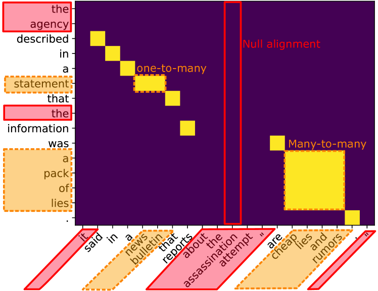
Figure 1 illustrates the challenges of monolingual word alignment. The first challenge is the null alignment, where words may not have corresponding counterparts, which causes alignment asymmetricity MacCartney et al. (2008). Null alignment is prevalent in semantically divergent sentences; indeed, the null alignment ratio reaches in entailment sentence pairs used in our experiments (shown in the third row of Table 2). Its identification explicitly declares semantic gaps between two sentences and helps reason about their semantic (dis)similarity Li and Srikumar (2016). The second challenge is that alignment beyond one-to-one mapping needs to be addressed. These challenges constitute an unbalanced word alignment problem, where both word-by-word and null alignment should be fully identified.
This study reveals that a family of optimal transport (OT) are suitable tools for unbalanced word alignment. Among the OT problems, balanced OT (BOT) Monge (1781); Kantorovich (1942)111We explicitly call it balanced OT (BOT) to distinguish it from partial and unbalanced OT in this paper. should be the most prominent in natural language processing (NLP) Wan (2007); Kusner et al. (2015), which can handle many-to-many alignment. In contrast to BOT that is unable to deal with null alignment, partial OT (POT) Caffarelli and McCann (2010); Figalli (2010) and unbalanced OT (UOT) Frogner et al. (2015); Chizat et al. (2016) can handle the asymmetricity as desired in unbalanced word alignment, which has also attracted applications where null alignment is unignorable Swanson et al. (2020); Zhang et al. (2020a); Yu et al. (2022); Chen et al. (2020b); Wang et al. (2020).
This is the first study that connects these two paradigms of unbalanced word alignment and the family of OT problems that can naturally address null alignment as well as many-to-many alignment. We empirically (1) demonstrate that the OT-based methods are natural and sufficiently powerful approaches to unbalanced word alignment without tailor-made techniques and (2) deliver a comprehensive picture that unveils the characteristics of BOT, POT, and UOT on unbalanced word alignment with different null alignment ratios. We conduct extensive experiments using representative datasets for understanding OT-based alignment: effects of OT formalisation, regularisation, and a heuristic to sparsify alignments. Our primary findings can be summarised as follows. First, in unsupervised alignment, the best OT problem depends on null alignment ratios. Second, simple thresholding on regularised BOT can produce unbalanced alignment. Third, in supervised alignment, simple and generic OT-based alignment shows competitive performance to the state-of-the-art models specially designed for word alignment.
The adoption of well-understood methods with a solid theory like OT is highly valuable in application development and scientific reproducibility. Furthermore, OT-based alignment performs superiorly or competitively to existing methods, despite being independent of tailor-made techniques. Our OT-based alignment methods are publicly available as a tool called OTAlign.222https://github.com/yukiar/OTAlign
2 Related Work
2.1 Word Alignment Problem
Word alignment techniques have been actively studied in the crosslingual setting, primarily for machine translation. Crosslingual and monolingual word alignment tackle relevant problems; however, they have notable differences MacCartney et al. (2008). Crosslingual alignment can assume that a large-scale parallel corpus exists, which is scarce in the monolingual case. Furthermore, asymmetricity can be more intense in monolingual alignment to handle semantically divergent sentences. A common approach to crosslingual word alignment is unsupervised learning using parallel corpora Och and Ney (2003); Dyer et al. (2013); Garg et al. (2019); Zenkel et al. (2020); Dou and Neubig (2021). Among them, Dou and Neubig (2021) applied BOT for alignment while focussing on fine-tuning multilingual pre-trained language models using a parallel corpus. Among crosslingual word alignment methods, SimAlign Jalili Sabet et al. (2020) is directly applicable to monolingual alignment because it only uses a multilingual pre-trained language model and simple heuristics without parallel corpora. In addition, the supervised word alignment method proposed by Nagata et al. (2020), which modelled alignment as a question-answering task, is also applicable.
For monolingual word alignment, supervised learning has been commonly used MacCartney et al. (2008); Thadani and McKeown (2011); Thadani et al. (2012a). A representative method modelled word alignment using the conditional random field regarding source words as observations and target words as hidden states Yao et al. (2013a, b). Lan et al. (2021) enhanced this approach by adopting neural models, which constitute the state-of-the-art methods together with Nagata et al. (2020). In monolingual alignment, phrase alignment is also a research focus Ouyang and McKeown (2019); Arase and Tsujii (2020); Culkin et al. (2021), which depends on high-quality parsers and chunkers. In contrast, we use words as an alignment unit and do not assume the availability of such parsers.
2.2 Optimal Transport in NLP
BOT, POT, and UOT have been adopted in various NLP tasks where alignment exists implicitly or explicitly. Most previous studies modelled tasks of their interest, with alignment being a hidden state; further, the alignment quality itself was out of their focus. A typical application is similarity estimation among sentences and documents using BOT Kusner et al. (2015); Huang et al. (2016); Zhao et al. (2019); Yokoi et al. (2020); Chen et al. (2020b); Alqahtani et al. (2021); Lee et al. (2022); Mysore et al. (2022); Wang et al. (2022) and recently UOT Chen et al. (2020b); Wang et al. (2020). Such similarity estimation mechanisms can be integrated into language generation models as a penalty Chen et al. (2019); Zhang et al. (2020b); Li et al. (2020).
Unlike the tasks above, alignment information obtained with BOT, POT, and UOT is the primary concern in extractive summarization Tang et al. (2022), text matching Swanson et al. (2020); Zhang et al. (2020a); Yu et al. (2022), and bilingual lexicon induction Zhang et al. (2017); Grave et al. (2019); Zhao et al. (2020). However, these tasks and unbalanced monolingual word alignment have different objectives. These tasks concern the precision where alignment exists. In contrast, unbalanced word alignment aims at exhaustive identification of both alignment and null alignment. Furthermore, there has not been any systematic study that compared the qualities of different OT-based alignment methods, which hinders the understanding of a suitable OT formulation for problems with different null alignment frequencies.
3 Problem Definition
Suppose we have a source and target sentence pair and with their word embeddings and , respectively, where . The goal of monolingual word alignment is to identify an alignment between semantically corresponding words, where indicates a likelihood or binary indicator of aligning and .
Evaluation Metrics for Unbalanced Alignment
As evaluation metrics, we adopt the macro averages of precision and recall of alignment pairs, and their F score MacCartney et al. (2008). In light of the importance of null alignment, we explicitly incorporate it into the evaluation metrics:
| precision | |||
| recall |
where and are sets of word-by-word alignment pairs in prediction and ground-truth, respectively, e.g., if aligns to . The sets of and correspond to those of null-alignment that regards a word aligning to a null word , e.g., if is null alignment. Hence, is equal to the number of null alignment words in the ground-truth. Compared to previous metrics that only consider and MacCartney et al. (2008), ours consider null alignment equally as word-by-word alignment.
4 Background: Optimal Transport
OT seeks the most efficient way to move mass from one measure to another. Remarkably, the OT problem induces the OT mapping that indicates correspondences between the samples. While OT is frequently used as a distance metric between two measures, OT mapping is often the primary concern in alignment problems.
Formally, the inputs to the optimal transport problem are a cost function and a pair of measures. On the premise of its application to monolingual word alignment, the following explanation assumes that the source and target sentences and and their word embeddings are at hand (see §3). A cost means a dissimilarity between and (source and target words) computed by a distance metric , such as Euclidean and cosine distances. The cost matrix summarises the costs of any word pairs, that is, . A measure means a weight each word has. The concept of measure corresponds to fertility introduced in IBM Model Brown et al. (1993), which defines how many target (source) words a source (target) word can align. In summary, the mass of words in and is represented as arbitrary measures and , respectively.333Subsequently, we use the terms mass and fertility interchangeably to indicate each element of measures. Finally, the OT problem identifies an alignment matrix with which the sum of alignment costs is minimised under the cost matrix :
| (1) |
where . The alignment matrix belongs to that is a set of valid alignment matrices, introduced in the following sections. With this formulation, we can seek the most plausible word alignment matrix .
4.1 Balanced Optimal Transport
BOT Kantorovich (1942) assumes that and are probability distributions, i.e., and , respectively, where is the probability simplex: . In this case, alignment matrices must live in the following space:
|
|
(2) |
where is the all-ones vector of size . Under this constraint set, the BOT problem is a linear programming (LP) problem and can be solved by standard LP solvers Pele and Werman (2009). However, the non-differentiable nature makes it challenging to integrate into neural models.
Regularised BOT
The entropy-regularised optimal transport Cuturi (2013), initially aimed at improving the computational speed of BOT, is a differentiable alternative and thus can be directly integrated into neural models. The regularisation makes the objective as follows:
| (3) |
where the function is the negative entropy of alignment matrix , and controls the strength of the regularisation; with sufficiently small , well approximates the exact BOT. The optimisation problem can be efficiently solved using the Sinkhorn algorithm Sinkhorn (1964).
4.2 Relaxation of BOT Constraint
Despite its success, the hard constraint of the BOT that aligns all words often makes it sub-optimal for some alignment problems where null alignment is more or less pervasive, such as unbalanced word alignment. POT and UOT introduced subsequently relax this constraint to allow certain words to be left unaligned.
Partial Optimal Transport
POT Caffarelli and McCann (2010); Figalli (2010) relaxes BOT by aligning only a fraction of the fertility, with the following constraint set in place of :
| (4) | ||||
| (5) |
The fraction is bound as where represents the norm. While POT can be solved by standard LP solvers, it can also be regularised as in the BOT and solved with the Sinkhorn algorithm Benamou et al. (2015).
Unbalanced Optimal Transport
UOT relaxes BOT by introducing soft constraints that penalise marginal deviation.
| (6) | ||||
| (7) |
where is a divergence and and control how much mass deviations are penalised. Notice that the unbalanced formulation seeks alignment matrices in the entire . In this study, we adopt the Kullback–Leibler divergence as because of its simplicity in computation Frogner et al. (2015); Chizat et al. (2016).
5 Proposal: Unbalanced Word Alignment as Optimal Transport Problem
In this study, we aim at formulating monolingual word alignment with high null frequencies in a natural way. For this purpose, we leverage OT with different constraints and reveal their features on this problem. We adopt the basic and generic cost matrices and measures instead of engineering them to avoid obfuscating the difference between BOT, POT, and UOT.
5.1 Cost Function and Measures
We obtain contextualised word embeddings from a pre-trained language model as adopted in the previous word alignment methods Jalili Sabet et al. (2020); Dou and Neubig (2021). Specifically, we concatenate source and target sentences and input to the language model to obtain the -th layer hidden outputs. We then compute a word embedding by mean pooling the hidden outputs of its subwords.
As a cost function, we use the cosine and Euclidean distances444Although the cosine distance is not a proper metric due to its in-satisfaction of the triangle inequality, we adopt it for its prevalence and empirical efficacy in NLP. to obtain the cost matrix , which are the most commonly used semantic dissimilarity metrics in NLP. In addition, we employ the distortion introduced in IBM Model Brown et al. (1993) when computing a cost to discourage aligning words appearing in distant positions. Jalili Sabet et al. (2020) modelled the distortion between and as , where scales the value to range in . The value becomes larger if the relative positions of and are largely different. Each entry of the cost matrix is then modulated by the corresponding distortion value. Note that the cost matrix is scaled in its computation process by using the min-max normalisation to make sure all entries lie in .555The scaling is not mathematically necessary; however, it is crucial for numerical stability in solving OT problems with the Sinkhorn algorithm; without the scaling, parameter tuning of becomes challenging as the relative scale of the alignment cost may deviate a lot.
Fertility determines the likelihood of words having alignment links. We use two standard measures adopted in previous studies that used OT in NLP tasks as discussed in §2.2: the uniform distribution Kusner et al. (2015) and -norms of word embeddings Yokoi et al. (2020). On POT and UOT, we directly use these measures without scaling, for which may have an arbitrary positive value. We scale by the min-max normalisation so that we can handle alignment matrices of BOT, POT, and UOT by a unified manner.
5.2 Heuristics for Sparse Alignment
While the Sinkhorn algorithm is a powerful tool for solving OT problems, one drawback is that a resultant alignment matrix becomes dense, i.e., each element has a non-zero weight. It is not straightforward to interpret a dense solution as an alignment matrix and thus dense matrices are better avoided. As an empirical remedy, simple heuristics have been commonly used to make alignment matrices sparse: assuming top- elements based on their mass Lee et al. (2022); Yu et al. (2022) or elements whose mass are larger than a threshold Swanson et al. (2020); Dou and Neubig (2021) are aligned.
We take the latter approach to avoid introducing an arbitrary assumption on fertility, i.e., the number of alignment links that a word can have. Specifically, we derive the final alignment matrix using a threshold :
| (8) |
Our experiments reveal that this simple ‘patch’ to obtain a sparse alignment can produce unbalanced alignment, rather than just sparse, as we see in §7.2.
5.3 Application to Unsupervised Alignment
We obtain contextualised word embeddings from a pre-trained masked language model without fine-tuning in the unsupervised setting. Such word embeddings are known to show relatively high cosine similarity between any random words Ethayarajh (2019), which blurs the actual similarity of semantically corresponding words. Chen et al. (2020a) alleviated this phenomenon with a simple technique of centring the word embedding distribution. We apply the corpus mean centring that subtracts the mean word vector of the entire corpus from each word embedding.
5.4 Application to Supervised Alignment
In the supervised alignment, we adopt linear metric learning Huang et al. (2016) that learns a matrix defining a generalised distance between two embeddings: . We train the entire model to learn parameters of and the pre-trained language model by minimising the binary cross-entropy loss:
|
|
(9) |
where and are the predicted and ground-truth alignment matrices, respectively. Specifically, indicates the ground-truth alignment between and ; means that alignment exists while means no alignment.
6 Experiment Settings
We empirically investigate the characteristics of BOT, POT, and UOT on word alignment in both unsupervised and supervised settings. We refer to our OT-based alignment methods as OTAlign, hereafter. To alleviate performance variations due to neural model initialisation, all the experiments were conducted for times with different random seeds, and the means of the scores are reported.
Dataset
| Train | Val | Test | ||
|---|---|---|---|---|
| MSR-RTE | ||||
| Edinburgh | ||||
| MultiMWA | MTRef | |||
| Wiki | ||||
| Newsela | – | – | ||
| ArXiv | – | – | ||
As datasets that provide human-annotated word alignment, we used Microsoft Research Recognizing Textual Entailment (MSR-RTE) Brockett (2007), Edinburgh Thadani et al. (2012b), and Multi-Genre Monolingual Word Alignment (MultiMWA) Lan et al. (2021) as shown in Table 1. MultiMWA consists of four subsets according to the sources of sentence pairs: MTRef, Newsela, ArXiv, and Wiki. Among them, Newsela and ArXiv are intended for a transfer-learning experiment, on which models trained using MTRef should be tested Lan et al. (2021). MSR-RTE and Edinburgh do not have an official split for validation. Hence, we subsampled a validation set from the training split, which was excluded from there. As the tradition of word alignment, there are two types of alignment links: sure and possible. The former indicates that an alignment was agreed upon by multiple annotators and thus preserves high confidence. Experiments were conducted in both ‘Sure and Possible’ and ‘Sure Only’ settings. For more details, see Appendix A.1.
Pre-trained Language Model
OTAlign as well as the recent powerful methods (§2.1) use contextualised word embeddings obtained from pre-trained (masked) language models. As the basic and standard model, we used BERT-base-uncased Devlin et al. (2019) for all the methods compared to directly observe the capabilities of different alignment mechanisms and to exclude performance differences owing to the underlying pre-trained models.666We indeed investigated the performance when adopting SpanBERT Joshi et al. (2020) as a pre-trained model. In summary, the results indicated that the underlying pre-trained model does not affect the overall trends of alignment methods, while their performance was consistently improved by a few percent owing to the better phrase representation. For unsupervised word alignment, we used the th layer in BERT that performs strongly in unsupervised textual similarity estimation Zhang et al. (2020c). For supervised alignment, we used the last hidden layer following the convention.
OTAlign
Our OT-based alignment methods require a cost function and fertility. As discussed in §5.1, we experiment with cosine and Euclidean distances as cost functions and uniform distribution and -norm of word embeddings as the fertility. Due to the space limitation, the main paper only discusses the results of a cost function and fertility that performed consistently strongly on the validation sets. Appendix B draws the complete picture of different distance metrics and fertility and analyses their effects. We fixed the regularisation penalty to throughout all experiments. The threshold to sparsify alignment matrices was searched in with interval to maximise the validation F. More details of the implementation and experiment environment are described in Appendix A.2.
7 Unsupervised Word Alignment
| Dataset (sparse dense) | MSR-RTE | Newsela | EDB | MTRef | Arxiv | Wiki | ||||||||
|---|---|---|---|---|---|---|---|---|---|---|---|---|---|---|
| Alignment links | S | S + P | S | S + P | S | S + P | S | S + P | S | S + P | S | |||
| Null alignment rate (%) | ||||||||||||||
| fast-align Dyer et al. (2013) | ||||||||||||||
| SimAlign Jalili Sabet et al. (2020) | ||||||||||||||
| Type | Reg. | cost | mass | |||||||||||
| BOT | – | cosine | uniform | |||||||||||
| Sk | cosine | uniform | ||||||||||||
| POT | – | cosine | uniform | |||||||||||
| Sk | cosine | uniform | ||||||||||||
| UOT | Sk | cosine | uniform | |||||||||||
We reveal features of OT-based methods on monolingual word alignment under unsupervised learning to segregate the effects of supervision on the pre-trained language model. Note that we use the validation sets for hyper-parameter tuning, which may not be strictly ‘unsupervised.’ We still call this scenario ‘unsupervised’ for convenience, believing that the preparation of small-scale annotation datasets should be feasible in most practical cases.
7.1 Settings
As a conventional word alignment method, we compared OTAlign to the fast-align Dyer et al. (2013) that implemented IBM Model . For fast-align, the training, validation, and test sets were concatenated and used to gather enough statistics for alignment. As the state-of-the-art unsupervised word alignment method, we compared OTAlign to SimAlign Jalili Sabet et al. (2020). While SimAlign was initially proposed for crosslingual word alignment, it is directly applicable to the monolingual setting. SimAlign computes a similarity matrix in the same manner as ours,777They use cosine similarity instead of distance. and aligns words using simple heuristics on the matrix. Specifically, we used the ‘IterMax’ that performed best across many language pairs. IterMax conducts the ‘ArgMax’ alignment iteratively (Jalili Sabet et al. (2020) set the iteration as two times), which aligns a word pair if their similarity is the highest among each other. SimAlign has two hyper-parameters: one for the distortion () and another for forcing null alignment if a word is not particularly similar to any target words. These values were tuned using the validation sets.
For OTAlign, POT has a hyper-parameter to represent a fraction of fertility to be aligned, which we parameterise as . UOT has marginal deviation penalties of and .888We set following the common trait to reduce the number of hyper-parameters Chapel et al. (2021). All of these hyper-parameters were searched in a range of with interval to maximise the validation F. For the distortion strength , we applied the same values tuned on SimAlign.
7.2 Results: Primary Observations
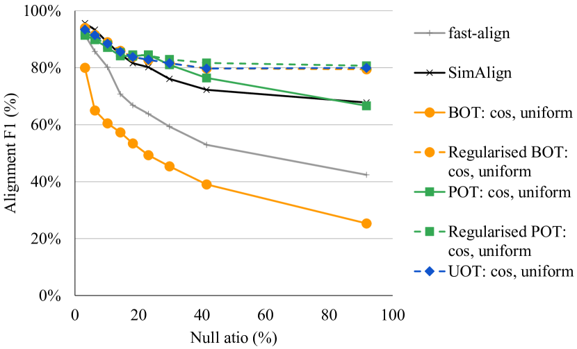
Table 2 shows the F scores measured on the test sets.999The complete sets of results including precision and recall are in Appendix B. We have the following observations: (i) The best OT problem depends on null alignment ratios. On datasets with higher null alignment ratios, i.e., Edinburgh and MTRef, regularised BOT, regularised POT, and UOT largely outperformed SimAlign. In particular, regularised POT performed the best on datasets with significantly high null alignment ratios, i.e., Newsela and MSR-RTE. On the other hand, when null alignment frequency is low, i.e., ArXiv and Wiki, regularised BOT, regularised POT, and UOT performed similarly. On these datasets, SimAlign also performed strongly thanks to the BERT representations.101010Table 4 in Appendix B shows that the simplest alignment by thresholding on a cosine similarity matrix using BERT embeddings outperforms SimAlign depending on datasets. (ii) Thresholding on the alignment matrix makes it unbalanced. As expected, the unregularised BOT showed the worst performance because its constraint forces to align all words and prohibits null alignment. In contrast, we observe that the performance of unregularised BOT and POT was significantly boosted by regularisation and thresholding on resultant alignment matrices (see the performance differences between with and without regulariser, denoted as ‘–’ and ‘Sk’, respectively, in Table 2).
For further investigation, we binned the test samples across datasets (under the ‘Sure Only’ setting) according to their null alignment ratios and observed the performance of the methods.111111Each bin had roughly the same number of samples. Figure 2 (a) shows the trend of the F score on all the datasets according to the null alignment ratios. Although the F score of BOT naturally degrades as null alignment rates increase, the F score of regularised BOT stays closer to that of UOT owing to thresholding on the regularised solutions. Similarly, the regularised POT outperforms the unregularised POT. Therefore, we argue that thresholding is vital to obtain not only a sparse but also unbalanced alignment matrix.
| Dataset (sparse dense) | MSR-RTE | Newsela | EDB | MTRef | Arxiv | Wiki | |||||||
| Alignment links | S | S + P | S | S + P | S | S + P | S | S + P | S | S + P | S | ||
| Null alignment rate (%) | |||||||||||||
| Lan et al. (2021) | |||||||||||||
| Nagata et al. (2020) | |||||||||||||
| Type | cost | mass | |||||||||||
| BOT | cosine | norm | |||||||||||
| POT | cosine | norm | |||||||||||
| UOT | cosine | norm | |||||||||||
Interestingly, most methods show a v-shape curve in Figure 2 (a), i.e., the F score decreases first and then increases again. We identified this trend is due to the characteristics of MSR-RTE. Most sentence pairs with a high () null alignment ratio come from MSR-RTE that consists of ‘hypothesis’ and ‘text’ of entailment pairs that tend to have largely different lengths. In these entailment pairs, most words in a (shorter) sentence would align with words in the (longer) pair, while the rest of the words in the pair have to be left unaligned. This characteristic is unique in MSR-RTE, which we conjecture affected the performance. In Figure 2 (b), we removed MSR-RTE and drew trends of the alignment F score. The alignment F approximately becomes inversely proportional to the null alignment rate as expected.
8 Supervised Word Alignment
In this section, we evaluate the performance of OTAlign in supervised word alignment by comparing it to the state-of-the-art methods.
8.1 Settings
We compared our OT-based alignment methods to the state-of-the-art supervised methods proposed by Lan et al. (2021) and Nagata et al. (2020). The method of Lan et al. (2021) uses a semi-Markov conditional random field combined with neural models to simultaneously conduct word and chunk alignment. Its high computational costs limit a chunk to be at most -gram. The method proposed by Nagata et al. (2020) models word alignment as span prediction in the same formulation as the SQuAD Rajpurkar et al. (2016) style question answering. These previous methods explicitly incorporate chunks in the alignment process. In contrast, our OT-based alignment is purely based on word-level distances represented as a cost matrix.
We trained alignment methods of the regularised BOT, regularised POT, and UOT in an end-to-end fashion using the Adafactor Shazeer and Stern (2018) optimiser. The batch size was set to for datasets except for Wiki, for which was used due to longer sentence lengths. The training was stopped early, with patience epochs and a minimum delta of based on the validation F score. Before evaluation, we searched the learning rate from with a interval using the validation sets. Other hyper-parameters were set to the same as the unsupervised settings.
8.2 Results
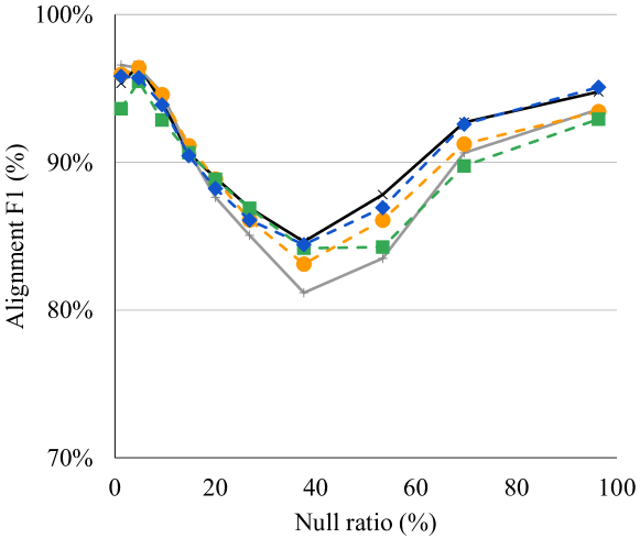
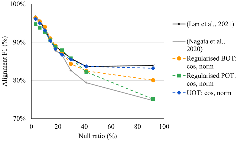
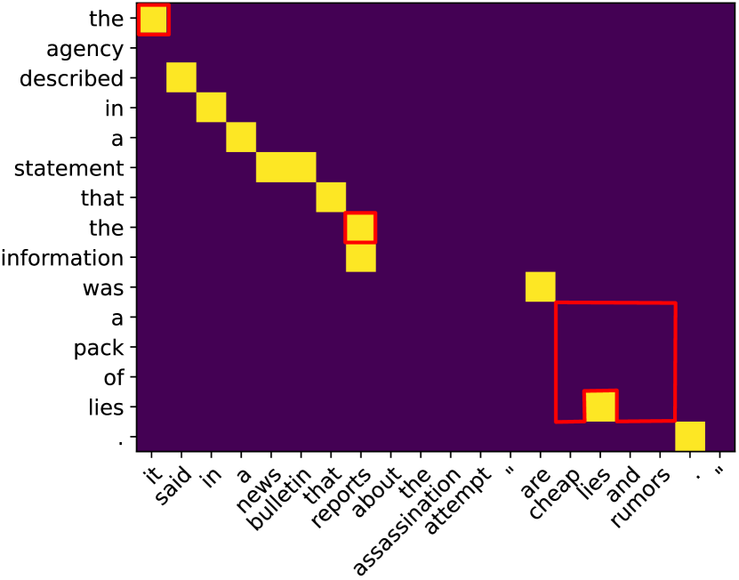
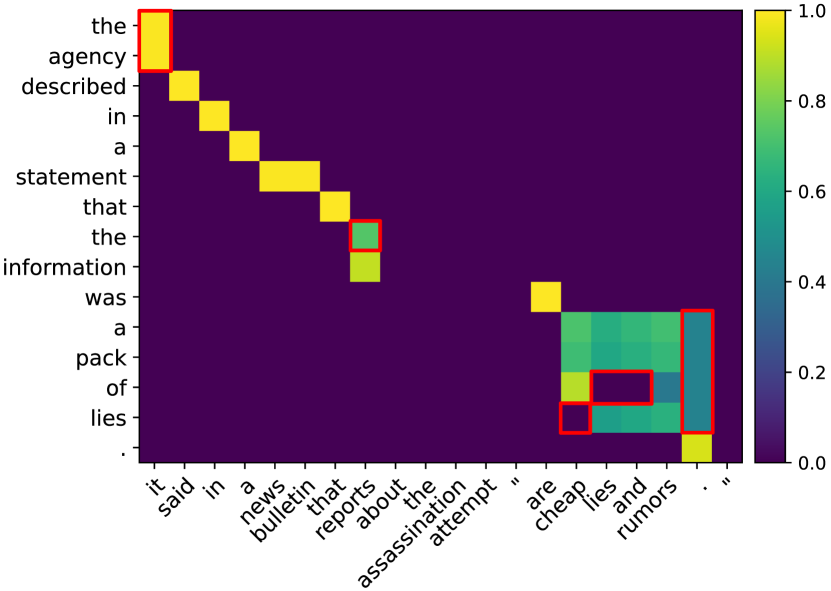
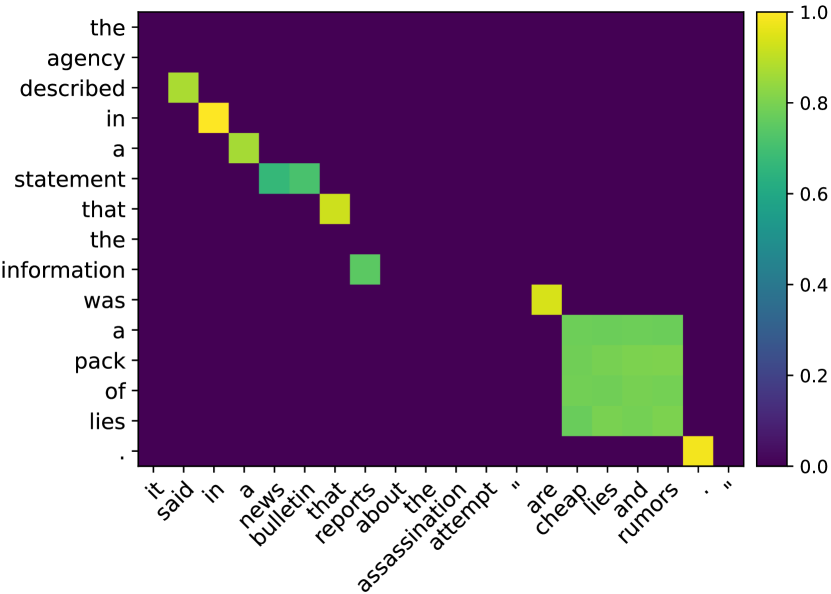
Table 3 shows the alignment F (%) measured on the test sets.121212The complete sets of results are available in Appendix B. The UOT-based alignment exhibits competitive performance against these state-of-the-art methods on the datasets with higher null alignment ratios. Notably, despite the simple and generic alignment mechanism based on UOT, it performed on par with Lan et al. (2021) who specially designed the model for monolingual word alignment. The UOT-based alignment also shows consistently higher alignment F scores compared to the regularised BOT and POT alignment. These results confirm that UOT well-captures the unbalanced word alignment problem. In addition, OT-based alignment showed better transferability as well as Lan et al. (2021) than Nagata et al. (2020) as demonstrated on results of Newsela and Arxiv. We conjecture this is because our cost matrix has less inductive bias due to its simplicity. In contrast, Nagata et al. (2020) directly learn to predict alignment spans.
Figure 3 shows the trend of the F score according to the null alignment ratios assembled in the same way as Figure 2. Figure 3 (a) shows the trend on all datasets, demonstrating the robustness of OT-based methods against null alignment. OT-based alignment outperformed Nagata et al. (2020) at sentences whose null alignment ratios are higher than . The performances of the regularised BOT and UOT reverse around null alignment ratio; the regularised BOT outperformed UOT on a lower side ( higher F on average except for the lowest edge) and UOT outperformed BOT on a higher side ( higher F on average). Same with the unsupervised word alignment, all methods show the v-shape trend. Figure 3 (b) shows the trend of the alignment F on the datasets except MSR-RTE. The performance of all methods becomes inversely proportional to the null alignment ratio as observed in the unsupervised case.
While UOT and previous methods are competitive on the datasets with high null alignment frequencies, we found that UOT has an advantage in longer phrase alignment. Figure 4 (a), (b), and (c) visualise alignment matrices by Lan et al. (2021), Nagata et al. (2020), and UOT, respectively, of the same sentence pair in Figure 1. The chunk size constraint in Lan et al. (2021), -gram at maximum, hindered the many-to-many alignment. Nagata et al. (2020) also failed to complete this alignment because their method conducts one-to-many alignment bidirectionally and merges results. In contrast, UOT can align such a long phrase pair if the cost matrix is sufficiently reliable as demonstrated here.
9 Summary and Future Work
This study revealed the features of BOT, POT, and UOT on unbalanced word alignment and suggested that they perform sufficiently powerfully without tailor-made designs. In future, our OT-based methods can be enhanced for better phrase alignment by employing sophisticated phrase embedding models as discussed in Limitations section. We will also apply OT-based alignment to problems related yet with different constraints and objectives, e.g., crosslingual word alignment and text matching.
Limitations
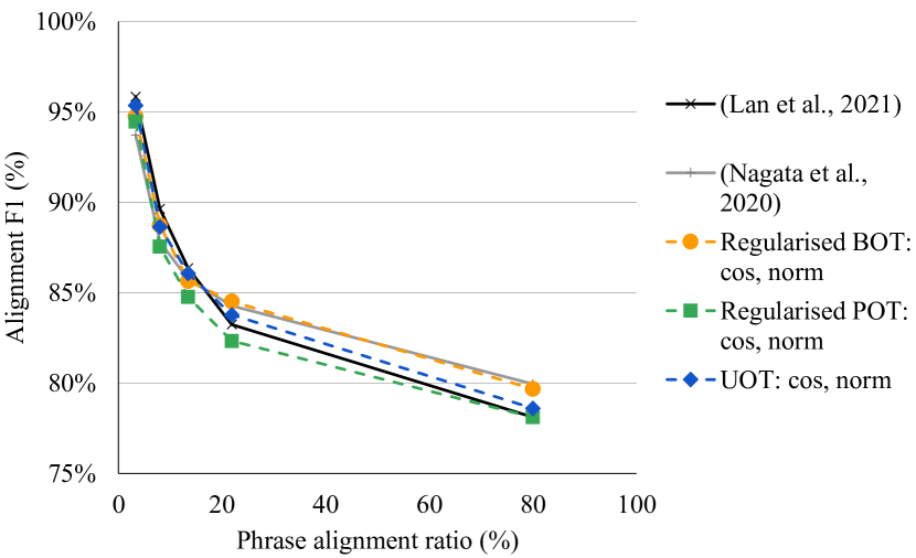
In this study, we used standard and basic word embeddings to highlight the characteristics of the different OT problems on unbalanced word alignment. This limits the capability of phrasal alignment. Similar to Figure 3 (a), we binned all the test samples across datasets (under the ‘Sure Only’ setting) according to their phrase alignment ratios and evaluated the performance of the supervised OT-based alignment methods.131313In the evaluation datasets, phrase alignment is infrequent, which skewed the bin sizes: the first bin (less than phrase alignment ratio) size was k and the rests were . Specifically, we regarded one-to-many, many-to-one, and many-to-many alignment as phrase alignment. Figure 5 shows the trend of the F score according to the phrase alignment ratios. Obviously, the F score degrades as more phrase alignment exists in a sentence pair.
One of the straightforward ways to improve the phrase alignment is exploring pre-trained language models enhanced for span representations Joshi et al. (2020) and sophisticated methods for phrase representation composition Yu and Ettinger (2020). In addition, phrase alignment can be addressed from the OT perspective, too, by conducting structure-aware Alvarez-Melis et al. (2018) and order-aware Liu et al. (2018) optimal transport. These directions constitute our future work.
Acknowledgements
We sincerely appreciate the anonymous reviewers for their insightful comments and suggestions to improve the paper. This work was partially supported by JSPS KAKENHI Grant Number 22H03654.
References
- Agirre et al. (2015) Eneko Agirre, Carmen Banea, Claire Cardie, Daniel Cer, Mona Diab, Aitor Gonzalez-Agirre, Weiwei Guo, Iñigo Lopez-Gazpio, Montse Maritxalar, Rada Mihalcea, German Rigau, Larraitz Uria, and Janyce Wiebe. 2015. SemEval-2015 task 2: Semantic textual similarity, English, Spanish and pilot on interpretability. In Proceedings of the International Workshop on Semantic Evaluation (SemEval), pages 252–263.
- Alqahtani et al. (2021) Sawsan Alqahtani, Garima Lalwani, Yi Zhang, Salvatore Romeo, and Saab Mansour. 2021. Using optimal transport as alignment objective for fine-tuning multilingual contextualized embeddings. In Findings of the Association for Computational Linguistics: EMNLP, pages 3904–3919.
- Alvarez-Melis et al. (2018) David Alvarez-Melis, Tommi Jaakkola, and Stefanie Jegelka. 2018. Structured optimal transport. In Proceedings of the International Conference on Artificial Intelligence and Statistics (AISTATS), volume 84 of Proceedings of Machine Learning Research, pages 1771–1780.
- Arase and Tsujii (2020) Yuki Arase and Jun’ichi Tsujii. 2020. Compositional phrase alignment and beyond. In Proceedings of the Conference on Empirical Methods in Natural Language Processing (EMNLP), pages 1611–1623.
- Bar-Haim et al. (2006) Roy Bar-Haim, Ido Dagan, Bill Dolan, Lisa Ferro, Danilo Giampiccolo, Bernardo Magnini, and Idan Szpektor. 2006. The second pascal recognising textual entailment challenge. In Proceedings of the PASCAL Challenges Workshop on Recognising Textual Entailment.
- Benamou et al. (2015) Jean-David Benamou, Guillaume Carlier, Marco Cuturi, Luca Nenna, and Gabriel Peyré. 2015. Iterative bregman projections for regularized transportation problems. SIAM Journal on Scientific Computing, 37(2):A1111–A1138.
- Brockett (2007) Chris Brockett. 2007. Aligning the RTE 2006 corpus. Technical Report MSR-TR-2007-77, Microsoft Research.
- Brook Weiss et al. (2021) Daniela Brook Weiss, Paul Roit, Ayal Klein, Ori Ernst, and Ido Dagan. 2021. QA-align: Representing cross-text content overlap by aligning question-answer propositions. In Proceedings of the Conference on Empirical Methods in Natural Language Processing (EMNLP), pages 9879–9894.
- Brown et al. (1993) Peter F. Brown, Stephen A. Della Pietra, Vincent J. Della Pietra, and Robert L. Mercer. 1993. The mathematics of statistical machine translation: Parameter estimation. Computational Linguistics, 19(2):263–311.
- Caffarelli and McCann (2010) Luis Caffarelli and Robert J. McCann. 2010. Free boundaries in optimal transport and monge-ampère obstacle problems. Annals of Mathematics, 171(2):673–730.
- Chapel et al. (2021) Laetitia Chapel, Rémi Flamary, Haoran Wu, Cédric Févotte, and Gilles Gasso. 2021. Unbalanced optimal transport through non-negative penalized linear regression. In Proceedings of Conference on Neural Information Processing Systems (NeurIPS), pages 23270–23282.
- Chen et al. (2019) Liqun Chen, Yizhe Zhang, Ruiyi Zhang, Chenyang Tao, Zhe Gan, Haichao Zhang, Bai Li, Dinghan Shen, Changyou Chen, and Lawrence Carin. 2019. Improving sequence-to-sequence learning via optimal transport. In Proceedings of the International Conference on Learning Representations (ICLR).
- Chen et al. (2020a) Xi Chen, Nan Ding, Tomer Levinboim, and Radu Soricut. 2020a. Improving text generation evaluation with batch centering and tempered word mover distance. In Proceedings of the Workshop on Evaluation and Comparison of NLP Systems, pages 51–59.
- Chen et al. (2020b) Yimeng Chen, Yanyan Lan, Ruinbin Xiong, Liang Pang, Zhiming Ma, and Xueqi Cheng. 2020b. Evaluating natural language generation via unbalanced optimal transport. In Proceedings of the International Joint Conference on Artificial Intelligence (IJCAI), pages 3730–3736.
- Chizat et al. (2016) Lenaic Chizat, Gabriel Peyré, Bernhard Schmitzer, and François-Xavier Vialard. 2016. Scaling algorithms for unbalanced transport problems. arXiv, 1607.05816.
- Culkin et al. (2021) Ryan Culkin, J. Edward Hu, Elias Stengel-Eskin, Guanghui Qin, and Benjamin Van Durme. 2021. Iterative paraphrastic augmentation with discriminative span alignment. Transactions of the Association of Computational Linguistics (TACL), 9:494–509.
- Cuturi (2013) Marco Cuturi. 2013. Sinkhorn distances: Lightspeed computation of optimal transport. In Proceedings of Conference on Neural Information Processing Systems (NeurIPS), volume 26.
- Dagan et al. (2006) Ido Dagan, Oren Glickman, and Bernardo Magnini. 2006. The pascal recognising textual entailment challenge. In Machine Learning Challenges. Evaluating Predictive Uncertainty, Visual Object Classification, and Recognising Tectual Entailment, pages 177–190.
- Das and Smith (2009) Dipanjan Das and Noah A. Smith. 2009. Paraphrase identification as probabilistic quasi-synchronous recognition. In Proceedings of the Joint Conference of the Annual Meeting of the Association for Computational Linguistics and the International Joint Conference on Natural Language Processing (ACL-IJCNLP), pages 468–476.
- Devlin et al. (2019) Jacob Devlin, Ming-Wei Chang, Kenton Lee, and Kristina Toutanova. 2019. BERT: Pre-training of deep bidirectional transformers for language understanding. In Proceedings of the Annual Conference of the North American Chapter of the Association for Computational Linguistics: Human Language Technologies (NAACL-HLT), pages 4171–4186.
- Dou and Neubig (2021) Zi-Yi Dou and Graham Neubig. 2021. Word alignment by fine-tuning embeddings on parallel corpora. In Proceedings of the Conference of the European Chapter of the Association for Computational Linguistics (EACL), pages 2112–2128.
- Dyer et al. (2013) Chris Dyer, Victor Chahuneau, and Noah A. Smith. 2013. A simple, fast, and effective reparameterization of IBM model 2. In Proceedings of the Annual Conference of the North American Chapter of the Association for Computational Linguistics: Human Language Technologies (NAACL-HLT), pages 644–648.
- Ethayarajh (2019) Kawin Ethayarajh. 2019. How contextual are contextualized word representations? Comparing the geometry of BERT, ELMo, and GPT-2 embeddings. In Proceedings of Conference on Empirical Methods in Natural Language Processing and the International Joint Conference on Natural Language Processing (EMNLP-IJCNLP), pages 55–65.
- Feldman and El-Yaniv (2019) Yair Feldman and Ran El-Yaniv. 2019. Multi-hop paragraph retrieval for open-domain question answering. In Proceedings of the Annual Meeting of the Association for Computational Linguistics (ACL), pages 2296–2309.
- Figalli (2010) Alessio Figalli. 2010. The optimal partial transport problem. Archive for Rational Mechanics and Analysis, 195(2):533–560.
- Flamary et al. (2021) Rémi Flamary, Nicolas Courty, Alexandre Gramfort, Mokhtar Z. Alaya, Aurélie Boisbunon, Stanislas Chambon, Laetitia Chapel, Adrien Corenflos, Kilian Fatras, Nemo Fournier, Léo Gautheron, Nathalie T.H. Gayraud, Hicham Janati, Alain Rakotomamonjy, Ievgen Redko, Antoine Rolet, Antony Schutz, Vivien Seguy, Danica J. Sutherland, Romain Tavenard, Alexander Tong, and Titouan Vayer. 2021. POT: Python optimal transport. Journal of Machine Learning Research, 22(78):1–8.
- Frogner et al. (2015) Charlie Frogner, Chiyuan Zhang, Hossein Mobahi, Mauricio Araya, and Tomaso A Poggio. 2015. Learning with a Wasserstein loss. In Proceedings of Conference on Neural Information Processing Systems (NeurIPS), volume 28.
- Garg et al. (2019) Sarthak Garg, Stephan Peitz, Udhyakumar Nallasamy, and Matthias Paulik. 2019. Jointly learning to align and translate with transformer models. In Proceedings of Conference on Empirical Methods in Natural Language Processing and the International Joint Conference on Natural Language Processing (EMNLP-IJCNLP), pages 4453–4462.
- Grave et al. (2019) Edouard Grave, Armand Joulin, and Quentin Berthet. 2019. Unsupervised alignment of embeddings with Wasserstein procrustes. In Proceedings of the International Conference on Artificial Intelligence and Statistics (AISTATS), pages 1880–1890.
- Heilman and Smith (2010) Michael Heilman and Noah A. Smith. 2010. Tree edit models for recognizing textual entailments, paraphrases, and answers to questions. In Proceedings of the Annual Conference of the North American Chapter of the Association for Computational Linguistics: Human Language Technologies (NAACL-HLT), pages 1011–1019.
- Hirsch et al. (2021) Eran Hirsch, Alon Eirew, Ori Shapira, Avi Caciularu, Arie Cattan, Ori Ernst, Ramakanth Pasunuru, Hadar Ronen, Mohit Bansal, and Ido Dagan. 2021. iFacetSum: Coreference-based interactive faceted summarization for multi-document exploration. In Proceedings of the Conference on Empirical Methods in Natural Language Processing: System Demonstrations, pages 283–297.
- Huang et al. (2016) Gao Huang, Chuan Guo, Matt J Kusner, Yu Sun, Fei Sha, and Kilian Q Weinberger. 2016. Supervised word mover's distance. In Proceedings of Conference on Neural Information Processing Systems (NeurIPS), volume 29.
- Jalili Sabet et al. (2020) Masoud Jalili Sabet, Philipp Dufter, François Yvon, and Hinrich Schütze. 2020. SimAlign: High quality word alignments without parallel training data using static and contextualized embeddings. In Findings of the Association for Computational Linguistics: EMNLP, pages 1627–1643.
- Jiang et al. (2020) Chao Jiang, Mounica Maddela, Wuwei Lan, Yang Zhong, and Wei Xu. 2020. Neural CRF model for sentence alignment in text simplification. In Proceedings of the Annual Meeting of the Association for Computational Linguistics (ACL), pages 7943–7960.
- Joshi et al. (2020) Mandar Joshi, Danqi Chen, Yinhan Liu, Daniel S. Weld, Luke Zettlemoyer, and Omer Levy. 2020. SpanBERT: Improving pre-training by representing and predicting spans. Transactions of the Association of Computational Linguistics (TACL), 8:64–77.
- Kantorovich (1942) L. V. Kantorovich. 1942. On the translocation of masses. Doklady Akademii Nauk, 37(2):227–229.
- Kusner et al. (2015) Matt Kusner, Yu Sun, Nicholas Kolkin, and Kilian Weinberger. 2015. From word embeddings to document distances. In Proceedings of the International Conference on Machine Learning (ICML), pages 957–966.
- Lan et al. (2021) Wuwei Lan, Chao Jiang, and Wei Xu. 2021. Neural semi-Markov CRF for monolingual word alignment. In Proceedings of the Joint Conference of the Annual Meeting of the Association for Computational Linguistics and the International Joint Conference on Natural Language Processing (ACL-IJCNLP), pages 6815–6828.
- Lee et al. (2022) Seonghyeon Lee, Dongha Lee, Seongbo Jang, and Hwanjo Yu. 2022. Toward interpretable semantic textual similarity via optimal transport-based contrastive sentence learning. In Proceedings of the Annual Meeting of the Association for Computational Linguistics (ACL), pages 5969–5979.
- Li et al. (2020) Jianqiao Li, Chunyuan Li, Guoyin Wang, Hao Fu, Yuhchen Lin, Liqun Chen, Yizhe Zhang, Chenyang Tao, Ruiyi Zhang, Wenlin Wang, Dinghan Shen, Qian Yang, and Lawrence Carin. 2020. Improving text generation with student-forcing optimal transport. In Proceedings of the Conference on Empirical Methods in Natural Language Processing (EMNLP), pages 9144–9156.
- Li and Srikumar (2016) Tao Li and Vivek Srikumar. 2016. Exploiting sentence similarities for better alignments. In Proceedings of the Conference on Empirical Methods in Natural Language Processing (EMNLP), pages 2193–2203.
- Liu et al. (2018) Bang Liu, Ting Zhang, Fred X. Han, Di Niu, Kunfeng Lai, and Yu Xu. 2018. Matching natural language sentences with hierarchical sentence factorization. In Proceedings of the World Wide Web Conference (WWW), page 1237–1246.
- MacCartney et al. (2008) Bill MacCartney, Michel Galley, and Christopher D. Manning. 2008. A phrase-based alignment model for natural language inference. In Proceedings of the Conference on Empirical Methods in Natural Language Processing (EMNLP), pages 802–811.
- Monge (1781) Gaspard Monge. 1781. Mémoire sur la théorie des déblais et des remblais. Histoire de l’Académie Royale des Sciences de Paris.
- Mysore et al. (2022) Sheshera Mysore, Arman Cohan, and Tom Hope. 2022. Multi-vector models with textual guidance for fine-grained scientific document similarity. In Proceedings of the Annual Conference of the North American Chapter of the Association for Computational Linguistics: Human Language Technologies (NAACL-HLT), pages 4453–4470.
- Nagata et al. (2020) Masaaki Nagata, Katsuki Chousa, and Masaaki Nishino. 2020. A supervised word alignment method based on cross-language span prediction using multilingual BERT. In Proceedings of the Conference on Empirical Methods in Natural Language Processing (EMNLP), pages 555–565.
- Och and Ney (2003) Franz Josef Och and Hermann Ney. 2003. A systematic comparison of various statistical alignment models. Computational Linguistics, 29(1):19–51.
- Ouyang and McKeown (2019) Jessica Ouyang and Kathy McKeown. 2019. Neural network alignment for sentential paraphrases. In Proceedings of the Annual Meeting of the Association for Computational Linguistics (ACL), pages 4724–4735.
- Pele and Werman (2009) Ofir Pele and Michael Werman. 2009. Fast and robust Earth Mover’s Distances. In Proceedings of International Conference on Computer Vision (ICCV), pages 460–467.
- Rajpurkar et al. (2016) Pranav Rajpurkar, Jian Zhang, Konstantin Lopyrev, and Percy Liang. 2016. SQuAD: 100,000+ questions for machine comprehension of text. In Proceedings of the Conference on Empirical Methods in Natural Language Processing (EMNLP), pages 2383–2392.
- Shapira et al. (2017) Ori Shapira, Hadar Ronen, Meni Adler, Yael Amsterdamer, Judit Bar-Ilan, and Ido Dagan. 2017. Interactive abstractive summarization for event news tweets. In Proceedings of the Conference on Empirical Methods in Natural Language Processing: System Demonstrations, pages 109–114.
- Shazeer and Stern (2018) Noam Shazeer and Mitchell Stern. 2018. Adafactor: Adaptive learning rates with sublinear memory cost. In Proceedings of the International Conference on Machine Learning (ICML), pages 4596–4604.
- Sinkhorn (1964) Richard Sinkhorn. 1964. A relationship between arbitrary positive matrices and doubly stochastic matrices. Annals of Mathematical Statistics, 35:876–879.
- Sultan et al. (2014) Md Arafat Sultan, Steven Bethard, and Tamara Sumner. 2014. Back to basics for monolingual alignment: Exploiting word similarity and contextual evidence. Transactions of the Association of Computational Linguistics (TACL), 2:219–230.
- Swanson et al. (2020) Kyle Swanson, Lili Yu, and Tao Lei. 2020. Rationalizing text matching: Learning sparse alignments via optimal transport. In Proceedings of the Annual Meeting of the Association for Computational Linguistics (ACL), pages 5609–5626.
- Tang et al. (2022) Peggy Tang, Kun Hu, Rui Yan, Lei Zhang, Junbin Gao, and Zhiyong Wang. 2022. OTExtSum: Extractive Text Summarisation with Optimal Transport. In Findings of the Association for Computational Linguistics: NAACL (Findings-NAACL), pages 1128–1141.
- Thadani et al. (2012a) Kapil Thadani, Scott Martin, and Michael White. 2012a. A joint phrasal and dependency model for paraphrase alignment. In Proceedings of the International Conference on Computational Linguistics (COLING), pages 1229–1238.
- Thadani et al. (2012b) Kapil Thadani, Scott Martin, and Michael White. 2012b. A joint phrasal and dependency model for paraphrase alignment. In Proceedings of the International Conference on Computational Linguistics (COLING), pages 1229–1238.
- Thadani and McKeown (2011) Kapil Thadani and Kathleen McKeown. 2011. Optimal and syntactically-informed decoding for monolingual phrase-based alignment. In Proceedings of the Annual Meeting of the Association for Computational Linguistics: Human Language Technologies (ACL-HLT), pages 254–259.
- Thadani and McKeown (2013) Kapil Thadani and Kathleen McKeown. 2013. Supervised sentence fusion with single-stage inference. In Proceedings of the International Joint Conference on Natural Language Processing (IJCNLP), pages 1410–1418.
- Wan (2007) Xiaojun Wan. 2007. A novel document similarity measure based on earth mover’s distance. Information Sciences, 177(18):3718–3730.
- Wang and Manning (2010) Mengqiu Wang and Christopher Manning. 2010. Probabilistic tree-edit models with structured latent variables for textual entailment and question answering. In Proceedings of the International Conference on Computational Linguistics (COLING), pages 1164–1172.
- Wang et al. (2022) Zihao Wang, Jiaheng Dou, and Yong Zhang. 2022. Unsupervised sentence textual similarity with compositional phrase semantics. In Proceedings of the International Conference on Computational Linguistics (COLING), pages 4976–4995.
- Wang et al. (2020) Zihao Wang, Datong Zhou, Ming Yang, Yong Zhang, Chenglong Rao, and Hao Wu. 2020. Robust document distance with Wasserstein-Fisher-Rao metric. In Proceedings of the Asian Conference on Machine Learning, volume 129, pages 721–736.
- Wolf et al. (2020) Thomas Wolf, Lysandre Debut, Victor Sanh, Julien Chaumond, Clement Delangue, Anthony Moi, Pierric Cistac, Tim Rault, Remi Louf, Morgan Funtowicz, Joe Davison, Sam Shleifer, Patrick von Platen, Clara Ma, Yacine Jernite, Julien Plu, Canwen Xu, Teven Le Scao, Sylvain Gugger, Mariama Drame, Quentin Lhoest, and Alexander Rush. 2020. Transformers: State-of-the-art natural language processing. In Proceedings of the Conference on Empirical Methods in Natural Language Processing: System Demonstrations, pages 38–45.
- Yao (2014) Xuchen Yao. 2014. Feature-driven Question Answering With Natural Language Alignment. Ph.D. thesis, Johns Hopkins University.
- Yao et al. (2013a) Xuchen Yao, Benjamin Van Durme, Chris Callison-Burch, and Peter Clark. 2013a. A lightweight and high performance monolingual word aligner. In Proceedings of the Annual Meeting of the Association for Computational Linguistics (ACL), pages 702–707.
- Yao et al. (2013b) Xuchen Yao, Benjamin Van Durme, Chris Callison-Burch, and Peter Clark. 2013b. Semi-Markov phrase-based monolingual alignment. In Proceedings of the Conference on Empirical Methods in Natural Language Processing (EMNLP), pages 590–600.
- Yokoi et al. (2020) Sho Yokoi, Ryo Takahashi, Reina Akama, Jun Suzuki, and Kentaro Inui. 2020. Word rotator’s distance. In Proceedings of the Conference on Empirical Methods in Natural Language Processing (EMNLP), pages 2944–2960.
- Yu and Ettinger (2020) Lang Yu and Allyson Ettinger. 2020. Assessing phrasal representation and composition in transformers. In Proceedings of the Conference on Empirical Methods in Natural Language Processing (EMNLP), pages 4896–4907.
- Yu et al. (2022) Weijie Yu, Liang Pang, Jun Xu, Bing Su, Zhenhua Dong, and Ji-Rong Wen. 2022. Optimal partial transport based sentence selection for long-form document matching. In Proceedings of the International Conference on Computational Linguistics (COLING), pages 2363–2373.
- Zenkel et al. (2020) Thomas Zenkel, Joern Wuebker, and John DeNero. 2020. End-to-end neural word alignment outperforms GIZA++. In Proceedings of the Annual Meeting of the Association for Computational Linguistics (ACL), pages 1605–1617.
- Zhang et al. (2017) Meng Zhang, Yang Liu, Huanbo Luan, and Maosong Sun. 2017. Earth mover’s distance minimization for unsupervised bilingual lexicon induction. In Proceedings of the Conference on Empirical Methods in Natural Language Processing (EMNLP), pages 1934–1945.
- Zhang et al. (2020a) Ruiyi Zhang, Changyou Chen, Xinyuan Zhang, Ke Bai, and Lawrence Carin. 2020a. Semantic matching for sequence-to-sequence learning. In Findings of the Association for Computational Linguistics: EMNLP, pages 212–222.
- Zhang et al. (2020b) Shuying Zhang, Tianyu Zhao, and Tatsuya Kawahara. 2020b. Topic-relevant response generation using optimal transport for an open-domain dialog system. In Proceedings of the International Conference on Computational Linguistics (COLING), pages 4067–4077.
- Zhang et al. (2020c) Tianyi Zhang, Varsha Kishore, Felix Wu, Kilian Q. Weinberger, and Yoav Artzi. 2020c. BERTScore: Evaluating text generation with bert. In Proceedings of the International Conference on Learning Representations (ICLR).
- Zhao et al. (2019) Wei Zhao, Maxime Peyrard, Fei Liu, Yang Gao, Christian M. Meyer, and Steffen Eger. 2019. MoverScore: Text generation evaluating with contextualized embeddings and earth mover distance. In Proceedings of Conference on Empirical Methods in Natural Language Processing and the International Joint Conference on Natural Language Processing (EMNLP-IJCNLP), pages 563–578.
- Zhao et al. (2020) Xu Zhao, Zihao Wang, Yong Zhang, and Hao Wu. 2020. A relaxed matching procedure for unsupervised BLI. In Proceedings of the Annual Meeting of the Association for Computational Linguistics (ACL), pages 3036–3041.
Appendix A Details of Evaluation Settings
A.1 Evaluation Datasets
MSR-RTE and Edinburgh have been commonly used for evaluating monolingual word alignment models Yao et al. (2013b); Sultan et al. (2014). MultiMWA is the newest dataset that provides a larger number of examples with improved inter-annotator agreements.
MSR-RTE annotated word alignment on sentence pairs for the PASCAL RTE challenge Dagan et al. (2006); Bar-Haim et al. (2006). Due to the nature of RTE pairs, the lengths of the source and target sentences tend to diverge, which results in a higher null-alignment ratio. In contrast, Edinburgh annotates word alignment on paraphrase pairs collected from machine translation (MT) references, novels, and news domains. MultiMWA annotated (or corrected the original) word alignment on (1) paraphrases extracted from multiple human references for MT evaluation Yao (2014) (MTRef), (2) simple and complex sentence pairs sampled from Newsela-Auto Jiang et al. (2020) constructed for text simplification (Newsela), (3) aligned sentences extracted from arXiv141414https://arxiv.org/ revision history (arXiv), and (4) aligned Wikipedia151515https://en.wikipedia.org/ sentences based on the edit histories (Wiki).
A.2 Implementation and Environment
All the BOT-, POT-, and UOT-based word alignment methods were implemented using PyTorch,161616https://pytorch.org/ PyTorch Lightning,171717https://www.pytorchlightning.ai/ Hugging Face Transformers Wolf et al. (2020), and Python Optimal Transport Flamary et al. (2021) libraries.
For the previous studies compared, we used the public implementations released by the authors with the necessary modifications. All the experiments were conducted on an NVIDIA Tesla V when GPU computation is needed.
Appendix B Additional Experimental Results
Tables 4 to 6 show the F, precision, and recall scores of unsupervised word alignment with all the cost functions (cosine and Euclidean distances) and measures (the uniform distribution and -norms). Tables 7 to 9 indicate those of supervised word alignment experiments.
B.1 Effects of Cost Function and Measures
Unsupervised Alignment
The th and th rows from the top of Table 4 show the F scores of naive baselines that determine word alignment on the cost matrix with simple thresholding. That is, these baselines align words whose costs are smaller than the threshold. Their results indicate that cosine distance consistently outperforms Euclidean distance when word embeddings are naively used to estimate semantic similarity.
The unregularised BOT and POT also prefer cosine distance as the cost function but their performances are more sensitive to measures, i.e., the uniform distribution outperformed the -norms. The effect of the measures is most pronounced on the regularised BOT, likely because the uniform fertility makes the threshold selection simple. In contrast, UOT and regularised POT are less sensitive to the measures, likely because of their internal mechanism to allow null alignment.
Supervised Alignment
As shown in Table 7, the UOT significantly improved over the unsupervised setting, outperforming the POT. In the supervised setting, UOT prefers the -norms to model fertility than the uniform distribution. We conjecture that the BERT with linear metric learning successfully learns to adapt norms of word embeddings to well represent the fertility of words.
| Dataset (sparse dense) | MSR-RTE | Newsela | EDB | MTRef | Arxiv | Wiki | ||||||||
|---|---|---|---|---|---|---|---|---|---|---|---|---|---|---|
| Alignment links | S | S + P | S | S + P | S | S + P | S | S + P | S | S + P | S | |||
| Null alignment rate (%) | ||||||||||||||
| fast-align Dyer et al. (2013) | ||||||||||||||
| SimAlign Jalili Sabet et al. (2020) | ||||||||||||||
| Type | Reg. | cost | mass | |||||||||||
| – | – | cosine | – | |||||||||||
| – | – | L2 | – | |||||||||||
| BOT | – | cosine | norm | |||||||||||
| – | cosine | uniform | ||||||||||||
| – | L2 | norm | ||||||||||||
| – | L2 | uniform | ||||||||||||
| Sk | cosine | norm | ||||||||||||
| Sk | cosine | uniform | ||||||||||||
| Sk | L2 | norm | ||||||||||||
| Sk | L2 | uniform | ||||||||||||
| POT | – | cosine | norm | |||||||||||
| – | cosine | uniform | ||||||||||||
| – | L2 | norm | ||||||||||||
| – | L2 | uniform | ||||||||||||
| Sk | cosine | norm | ||||||||||||
| Sk | cosine | uniform | ||||||||||||
| Sk | L2 | norm | ||||||||||||
| Sk | L2 | uniform | ||||||||||||
| UOT | Sk | cosine | norm | |||||||||||
| Sk | cosine | uniform | ||||||||||||
| Sk | L2 | norm | ||||||||||||
| Sk | L2 | uniform | ||||||||||||
| Dataset (sparse dense) | MSR-RTE | Newsela | EDB | MTRef | Arxiv | Wiki | |||||||
|---|---|---|---|---|---|---|---|---|---|---|---|---|---|
| Alignment links | S | S + P | S | S + P | S | S + P | S | S + P | S | S + P | S | ||
| Null alignment rate (%) | |||||||||||||
| Lan et al. (2021) | |||||||||||||
| Nagata et al. (2020) | |||||||||||||
| Type | cost | mass | |||||||||||
| BOT | cosine | norm | |||||||||||
| cosine | uniform | ||||||||||||
| L2 | norm | ||||||||||||
| L2 | uniform | ||||||||||||
| POT | cosine | norm | |||||||||||
| cosine | uniform | ||||||||||||
| L2 | norm | ||||||||||||
| L2 | uniform | ||||||||||||
| UOT | cosine | norm | |||||||||||
| cosine | uniform | ||||||||||||
| L2 | norm | ||||||||||||
| L2 | uniform | ||||||||||||