Professional Basketball Player Behavior Synthesis via Planning with Diffusion

Abstract

Dynamically planning in multi-agent systems has been explored to improve decision-making in various domains (e.g., traffic flow management, sports strategy development). Professional basketball serves as a compelling example of a dynamic spatio-temporal game, encompassing both concealed strategic policies and context-dependent decision-making. However, processing the diverse on-court signals and navigating the vast space of potential actions and outcomes makes it difficult for existing approaches to swiftly identify optimal strategies in response to evolving circumstances. In this study, we first formulate the sequential decision-making process as a conditional trajectory generation process. Based on the formulation, we introduce PlayBest (PLAYer BEhavior SynThesis), a method for enhancing player decision-making. We extend the state-of-the-art generative model, diffusion probabilistic model, to learn challenging multi-agent environmental dynamics from historical National Basketball Association (NBA) player motion tracking data. To incorporate data-driven strategies, an auxiliary value function is trained using the play-by-play data with corresponding rewards acting as the plan guidance. To accomplish reward-guided trajectory generation, conditional sampling is introduced to condition the diffusion model on the value function and conduct classifier-guided sampling. We validate the effectiveness of PlayBest via comprehensive simulation studies from real-world data, contrasting the generated trajectories and play strategies with those employed by professional basketball teams. Our results reveal that the model excels at generating high-quality basketball trajectories that yield efficient plays, surpassing conventional planning techniques in terms of adaptability, flexibility, and overall performance. Moreover, the synthesized play strategies exhibit a remarkable alignment with professional tactics, highlighting the model’s capacity to capture the intricate dynamics of basketball games.

1 Introduction

The exploration of multi-agent dynamic systems and their planning has broad applicability across various domains. Whether it involves developing strategies for team sports, managing traffic flow, coordinating autonomous vehicles, or understanding the dynamics of financial markets, these scenarios can be effectively framed as multi-agent systems characterized by intricate interactions and decision-making processes. The ability to comprehend and plan within these systems becomes crucial for attaining optimal outcomes. Basketball, with its high level of dynamism and complexity as a team sport, serves as a captivating illustration of a real-time multi-agent dynamic system with intricate tactical elements. A basketball game requires continuous adaptation and strategic decision-making. Coaches and players rely on pertinent environmental and behavioral cues including teammates’ and opponents’ current positions and trajectories to select play strategies that respond effectively to opponents’ actions and adapt to real-time situational changes. Existing methods in sports analytics and trajectory optimization (Wang et al., 2018; Terner & Franks, 2020; Wang et al., 2022b) have made progress in modeling and predicting player movements and game outcomes. However, these approaches struggle to capture the intricate dynamics of basketball games and produce flexible, adaptive play strategies that can handle the uncertainties and complexities inherent in the sport. The challenges arise from the following two features of basketball games:

Modeling the complex environmental dynamics. Capturing the environmental dynamics in basketball games is a very challenging task due to the inherent complexity of the game, e.g., rapid changes in game situations and numerous possible actions at any given moment. The spatio-temporal nature of basketball data, including multiple player positions and ball trajectories, further complicates the modeling process. The need for a computationally efficient and scalable approach to handle the massive amounts of data generated during basketball games presents a major challenge for modeling environmental dynamics.

Reward Sparsity. An additional challenge lies in addressing reward sparsity. Unlike other reinforcement learning (RL) environments where immediate feedback is readily available after each action, basketball games often see long sequences of actions leading up to a single reward event (e.g., the scoring of a basket). This results in a sparse reward landscape, as many actions contribute indirectly to the final outcome but are not themselves immediately rewarded. This scenario complicates the learning process as it becomes more challenging for the planning algorithm to accurately attribute the impact of individual actions to the final reward. Designing effective methods to address the reward sparsity challenge remains a significant hurdle in applying typical planning algorithms to basketball and similar sports games.

Recently, powerful trajectory optimizers that leverage learned models often produce plans that resemble adversarial examples rather than optimal trajectories (Talvitie, 2014; Ke et al., 2019). In contrast, modern model-based RL algorithms tend to draw more from model-free approaches, such as value functions and policy gradients (Wang et al., 2019), rather than utilizing the trajectory optimization toolbox. Methods that depend on online planning typically employ straightforward gradient-free trajectory optimization techniques like random shooting (Nagabandi et al., 2018) or the cross-entropy method (Botev et al., 2013; Chua et al., 2018) to circumvent the above problems.

In this work, we first formulate the planning problem in basketball as a multi-player behavior synthesis task, and instantiate the behavior synthesis task as a trajectory generation task. Following the recent success of generative models in applications of single-agent planning (Janner et al., 2022; Ajay et al., 2022), we propose a novel application of the diffusion model called PlayBest (PLAYer BEhavior SynThesis), to generate optimal basketball trajectories and synthesize adaptive play strategies. Under most circumstances, the diffusion model serves as a generative model to capture the distribution of the input samples. In our study, we extend it as a powerful technique to enable flexible behavior synthesis in dynamic and uncertain multi-agent environments. The diffusion process explores different potential trajectories and adapts to changes in the environment through the iterative sampling process to model basketball court dynamics. To guide the reverse diffusion process with rewards, PlayBest features a value guidance module that guides the diffusion model to generate optimal play trajectories by conditional sampling. This integration naturally forms a conditional generative process, and it allows PlayBest to swiftly adapt to evolving conditions and pinpoint optimal solutions in real-time.

We instantiate PlayBest in a variety of simulation studies and real-world scenarios, demonstrating the effectiveness of PlayBest in generating high-quality basketball trajectories that yield effective plays. Extensive results reveal that our proposed approach outperforms conventional planning methods in terms of adaptability, flexibility, and overall performance, showing a remarkable alignment with professional basketball tactics.

The core contributions of this work are summarized as follows:

• We attempt to formulate the basketball player behavior synthesis problem as a guided sampling/conditional generation of multiple players and ball trajectories from diffusion models.

• We propose PlayBest, a framework featuring a diffusion probabilistic model with a value function, to instantiate the conditional generative model. We adapt the model to integrate multi-player behaviors and decisions in basketball and show that a number of desirable properties are obtained.

• We showcase the effectiveness of PlayBest via both quantitative and qualitative studies of the trajectories generated and validate the practicality of adopting PlayBest to investigate real basketball games.

2 Preliminary

In this section, we introduce key concepts of diffusion models and the notations in this paper. We then formally define the problem of professional basketball player behavior synthesis. We present a learning-based approach to planning, which is inspired by prior research on behavioral synthesis using trajectory optimization (Witkin & Kass, 1988; Tassa et al., 2012; Janner et al., 2022; Ajay et al., 2022). Afterwards, we provide an overview of the problem setting considered by trajectory optimization and discuss the diffusion probabilistic models utilized for this purpose.

2.1 Diffusion Probabilistic Models

Diffusion probabilistic models (Sohl-Dickstein et al., 2015; Ho et al., 2020) define the data-generating process as an iterative denoising procedure $p_{\theta}(\bm{\tau}^{i-1}\mid\bm{\tau}^{i})$. This denoising process reverses a forward diffusion process $q(\bm{\tau}^{i}\mid\bm{\tau}^{i-1})$ that progressively adds noise to corrupt the data structure. The data distribution induced by the model is derived as:

$$p_{\theta}(\bm{\tau}^{0})=\int p(\bm{\tau}^{N})\prod_{i=1}^{N}p_{\theta}(\bm{\tau}^{i-1}\mid\bm{\tau}^{i})\mathrm{d}\bm{\tau}^{1:N},$$ (1)

where $p(\bm{\tau}^{N})$ is a standard Gaussian prior, and $\bm{\tau}^{0}$ denotes training data. The model parameters $\theta$ are optimized by minimizing a variational bound on the negative log-likelihood of the reverse process:

$$\theta^{*}=\operatorname*{arg\,min}_{\theta}-\mathbb{E}_{\bm{\tau}^{0}}\left[\log p_{\theta}(\bm{\tau}^{0})\right].$$ (2)

Typically, the reverse process is parameterized as a Gaussian with fixed timestep-dependent covariances:

$$p_{\theta}(\bm{\tau}^{i-1}\mid\bm{\tau}^{i})=\mathcal{N}(\bm{\tau}^{i-1}\mid\mu_{\theta}(\bm{\tau}^{i},i),\Sigma^{i}).$$ (3)

The forward process $q(\bm{\tau}^{i}\mid\bm{\tau}^{i-1})$ is generally prespecified.

2.2 Trajectory Optimization Problem Setting

We consider a discrete-time system with dynamics $\mathbf{s}_{t+1}={\bm{f}}(\mathbf{s}_{t},\mathbf{a}_{t})$, where $\mathbf{s}_{t}$ represents the state and $\mathbf{a}_{t}$ denotes the action. Trajectory optimization aims to find a sequence of actions $\mathbf{a}_{0:T}^{*}$ that maximizes (or minimizes) an objective $\mathcal{J}$, factoring in per-timestep rewards $r(\mathbf{s}_{t},\mathbf{a}_{t})$:

$$\mathbf{a}_{0:T}^{*}=\operatorname*{arg\,max}_{\mathbf{a}_{0:T}}\mathcal{J}(\mathbf{s}_{0},\mathbf{a}_{0:T})=\operatorname*{arg\,max}_{\mathbf{a}_{0:T}}\sum_{t=0}^{T}r(\mathbf{s}_{t},\mathbf{a}_{t})$$ (4)

where $T$ refers to the planning horizon. We use the abbreviation $\bm{\tau}=(\mathbf{s}_{0},\mathbf{a}_{0},\mathbf{s}_{1},\mathbf{a}_{1},\ldots,\mathbf{s}_{T},\mathbf{a}_{T})$ for a trajectory containing interleaved states and actions, and $\mathcal{J}(\bm{\tau})$ represents the objective value of the trajectory.

Notation: In this study, two distinct "times" are considered: the time involved in the diffusion process, and the time relevant to the planning problem. Superscripts (default to $i$ if not specified) signify the timestep in the diffusion process, while subscripts (default to $t$ if not specified) indicate the timestep in the planning problem. To illustrate, $\mathbf{s}_{t}^{0}$ represents the state at the $t^{\text{th}}$ timestep in a trajectory devoid of noise. In cases where the context is clear, superscripts of noise-free quantities are excluded, such that $\bm{\tau}$ equates to $\bm{\tau}^{0}$. To enrich the notation, we occasionally refer to the $t^{\text{th}}$ state (or action) in a trajectory $\bm{\tau}$ as $\bm{\tau}_{\mathbf{s}_{t}}$ (or $\bm{\tau}_{\mathbf{a}_{t}}$).

2.3 Problem Description

The input for PlayBest consists of a set of basketball game records, denoted as $\mathcal{D}_{raw}$. These game records are composed of distinct elements, described as follows:

Motion Track Data. The motion track data, represented as $\mathcal{D}^{move}$, comprises static snapshots of in-game events, detailing the positions of all players and the ball at a rate of 25 frames per second. A game’s progression can be reconstructed and visualized using these snapshots.

Play-by-Play Data. Denoted as $\mathcal{D}^{pbp}$, the play-by-play data offers a game transcript in the form of possessions. This data includes 1) the possession timestamp, 2) the player initiating the possession, 3) the result of the possession (e.g., points scored), and 4) additional unique identifiers employed for possession categorization.

To facilitate learning, we divide $\mathcal{D}_{raw}$ into $\mathcal{D}_{train}$ and $\mathcal{D}_{test}$, representing the training and testing sets, based on gameplay timestamps. We formally define our task as follows:

Given a set of game records $\mathcal{D}_{train}=\mathcal{D}_{train}^{move}\cup\mathcal{D}_{train}^{pbp}$ and a reward function $\mathcal{J}_{\phi}$, with $\mathcal{J}_{\phi}$ depending on the reward definition given by the discriminative rules applied to $\mathcal{D}_{train}^{pbp}$, the objective is to generate trajectories $\{\bm{\tau}\}$ leaning towards the higher-reward regions of the state-action space. In essence, our goal is to develop a policy $\pi_{\theta,\phi}(\mathbf{a}\mid\mathbf{s})$, parameterized by $\theta$ and $\phi$, that determines the optimal action based on the states associated with each frame in $\mathcal{D}_{test}^{move}$.

3 The PlayBest Framework

In this section, we describe in detail how our framework is designed. We first give an overview and then present details of the model architecture including the diffusion and value function modules.

Figure 1: Overview framework of PlayBest. The overall pipeline can be split into four major components: Frame Labeling, Environmental Dynamics Learning, Value (Perturb) Function Training, and Trajectory Generation Guided by a Reward Function. The diffusion probabilistic model $\epsilon_{\theta}$ is trained to model the environmental dynamics. The reward predictor $\mathcal{J}_{\phi}$ is trained on the same trajectories as the diffusion model. During guided trajectory generation, our model takes both environmental dynamics and rewards as input, performs guided planning via conditional sampling, and generates the trajectories as the guided plan.

Framework Overview. Figure 1 depicts the PlayBest pipeline. The historical game replay data originates from actual games played during the 2015-2016 NBA regular season. Each team competes per their unknown policies $\pi_{\beta}$. The raw game data encompasses multiple modalities, and a game is characterized by a series of high-frequency snapshots (e.g., 25 frames per second). At any given time $t$, a snapshot includes an image displaying all player and ball positions, as well as additional metadata like the results of each possession (shot made/miss, free-throw made/miss, rebound, foul, turnover, etc), shot clock, and game clock at time $t$.

Out of the historical game replay data, we construct the player trajectories and ball trajectories to create the trajectory dataset $\mathcal{D}^{move}$. We then use the trajectory dataset $\mathcal{D}_{train}^{move}$ to train a diffusion model $\epsilon_{\theta}$ that aims at modeling the distribution of the 3-dimensional player and ball movements. The training process of the diffusion model mimics the training procedure of what is usually referred to as offline RL, where there is no online environment to interact with. However, the diffusion model by itself can only generate “like-real” trajectories that do not necessarily lead to a goal-specific outcome. To further generate trajectories that can represent “good plans”, we train a value function that maps any possible trajectory to its expected return. During the sampling stage, the mean of the diffusion model is perturbed by the gradient of the value function. In this way, the guided sampling is capable of generating the trajectories biased towards the high-reward region. Incorporating a diffusion model in planning problems not only enhances efficient exploration and resilience in volatile environments, but also addresses the challenge of long-horizon planning, enabling the generation of strategic, noise-reduced trajectories over extended periods.

In essence, our framework utilizes a dataset $\mathcal{D}$ collected by an unknown behavior policy $\pi_{\beta}$, which can be approximated as the “average" policy for all NBA teams. This dataset is gathered once and remains unaltered during training. The training process relies entirely on the training set $\mathcal{D}_{\text{train }}$ and does not interact with the environment. Upon completion of training, we anticipate that $\pi_{\theta}$ will exhibit strong generalization on $\mathcal{D}_{\text{test}}$.

3.1 Environmental Dynamics Modeling with Diffusion

(a) The shape of the training data. Trajectories are represented by the $(x,y,z)$ coordinates of the ten on-court players across two teams and the ball (11 channels). The action is made up of the momentum of each object at the same timestep.

(b) The general structure of the diffusion model $\epsilon_{\theta}$ is implemented by a U-net with temporal convolutional blocks, which have been widely utilized in image-centric diffusion models.

Figure 2: (a, b) The input and diffusion architecture.

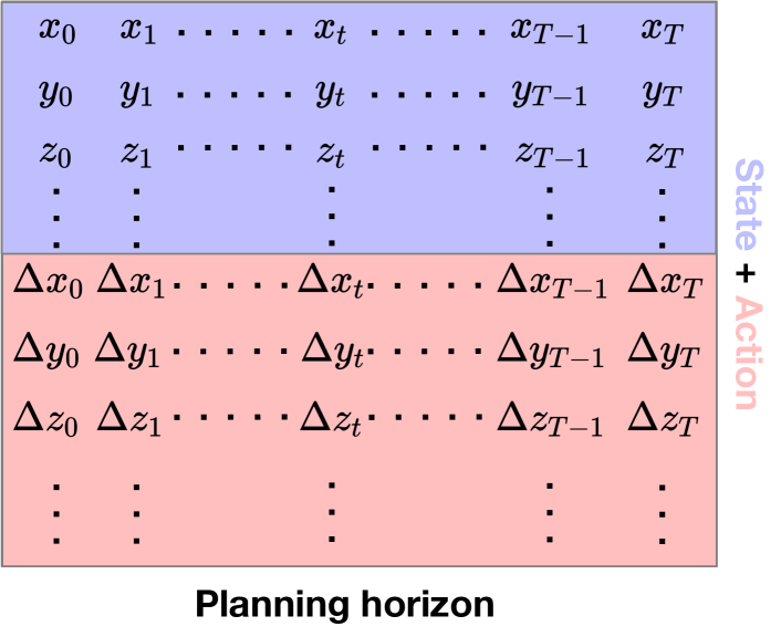
Model Input and Output. To represent our input that can be consumed by the diffusion model, we represent all the trajectories in the format of a 2-dimensional image as described in Figure 2(a). To be specific, we concatenate the state features and action features at each timestep in the game together to form one column of the model input. The features from different timesteps are then stacked together following the temporal order to form the rows. In other words, the rows in the model input correspond to the planning horizon $T$ in Section 2.2.

Architecture. As illustrated in Figure 2(b), the backbone of the environmental dynamics modeling module is a diffusion probabilistic model $\epsilon_{\theta}$. Diffusion models have been found effective in fitting the distribution of images (Ho et al., 2020). Our assumption is that the diffusion models can also learn the underlying distribution of basketball player trajectories by framing as the trajectory optimization problem, thereby modeling the player and ball dynamics. Following image-based diffusion models, we adopt the U-net architecture (Ronneberger et al., 2015) as the overall architecture. Moreover, to account for the temporal dependencies between different timesteps of the trajectories, we replace two-dimensional spatial convolutions with one-dimensional temporal convolutions.

Diffusion Training. To learn the parameters $\theta$, we parameterize the Gaussian noise term to make it predict $\epsilon_{t}$ from the input $x_{t}$ at diffusion step $t$:

$$\mathcal{L}(\theta)=\mathbb{E}_{t,\epsilon_{t},\bm{\tau}^{0}}\left[\lVert\epsilon_{t}-\epsilon_{\theta}(\bm{\tau}^{t},t)\rVert^{2}\right],$$ (5)

where $t\sim\mathcal{U}\{1,2,\ldots,N\}$ represents the diffusion step, $\epsilon_{t}\sim\mathcal{N}(\bm{0},\bm{I})$ denotes the noise target, and $\bm{\tau}^{t}$ is the trajectory $\bm{\tau}^{0}$ corrupted by noise $\epsilon$ at diffusion step $t$. From $\epsilon_{\theta}$, the mean $\mu_{\theta}$ can be solved in closed form (Ho et al., 2020).

3.2 Value (Perturb) Function Training for Reward Model

At the heart of the value function is an encoder that takes the trajectory data as input and returns the estimated cumulative reward. The structure of the return predictor $\mathcal{J}_{\phi}$ takes exactly the first half of the U-Net employed in the diffusion model, and it is followed by a linear layer that generates a single scalar output indicating the reward value.

3.3 Reward-guided Planning as Conditional Sampling

Existing studies (Janner et al., 2022; Ajay et al., 2022) have revealed the connections between classifier-guided / classifier-free sampling and reinforcement learning. The sampling routine of PlayBest resembles the classifier-guided sampling. In detail, we condition a diffusion model $p_{\theta}(\bm{\tau})$ on the states and actions encompassed within the entirety of the trajectory data. Following this, we develop an isolated model, $\mathcal{J}_{\phi}$, with the aim of forecasting the aggregated rewards of trajectory instances $\bm{\tau}^{i}$. The trajectory sampling operation is directed by the gradients of $\mathcal{J}_{\phi}$, which adjust the means $\mu$ of the reverse process as per the following equations:

$$\mu\leftarrow\mu_{\theta}\left(\bm{\tau}^{i}\right),$$ (6)

$$\bm{\tau}^{i-1}\sim\mathcal{N}\left(\mu+\alpha\Sigma\nabla\mathcal{J}_{\phi}(\mu),\Sigma^{i}\right),$$

$$\bm{\tau}_{\bm{s0}}^{i-1}\leftarrow\bm{s},$$

where $\alpha$ is the scaling factor to measure the impact of the guidance on the sampling, and

$$\nabla\mathcal{J}(\mu)=\left.\sum_{t=0}^{T}\nabla_{\mathbf{s}_{t},\mathbf{a}_{t}}r\left(\mathbf{s}_{t},\mathbf{a}_{t}\right)\right|_{\left(\mathbf{s}_{t},\mathbf{a}_{t}\right)=\mu_{t}}.$$ (7)

The detailed algorithm of reward-guided planning is illustrated in Appendix A.1

4 Experiments

We first give a thorough description of the dataset, then discuss the experimental settings including the input and output specifications and evaluation metrics. We report the overall performance, followed by a detailed analysis. Finally, we share our observations and insights gained from the experiments.

4.1 Experimental Setup

To quantitatively evaluate the effectiveness of player behavior planning, we focus on measuring the cumulative return given by the learned policy, which serves as an objective evaluation metric to compare the performance of PlayBest with other comparative methods. Evaluating offline RL is inherently difficult as it lacks real-time environment interaction for reward accumulation. Thus the model verification is primarily reliant on utilizing existing replay data. To validate the capacity of our framework in learning efficient tactics, we assess PlayBest’s ability to generate efficient plans using diverse data of varying standards.

# Training Games	# Minutes	# Plays	# Frames
480	23, 040	210, 952	34, 560, 000
# Testing Games	# Minutes	# Plays	# Frames
151	7, 248	68, 701	10, 872, 000
# Games	# Minutes	# Plays	# Frames
631	30, 288	279, 653	45, 432, 000

Table 1: NBA 2015 - 16 Regular Season Game Stats. Games are split chronically so that all the games in the test set happen after any game in the training set.

Event type	Reward
"start of period"	0
"jump ball"	0
"rebound"	0.25
"foul"	-0.25
"turnover"	-1
"timeout"	0
"substitution"	0
"end of period"	0
"violation"	-0.25
"3 pointer made"	3
"2 pointer made"	2
"free-throw made"	1

Table 2: Reward definition.

Dataset. We obtained our data from an open-source repository (spo, 2016; pbp, 2016). The model’s input data is a combination of two components: (1) Player Movement Sensor Data: This component captures real-time court events, detailing the positions of the players and the ball in Cartesian coordinates. The sampling frequency of this data is 25 frames per second. The statistics are detailed in Table 2. (2) Play-by-Play: This segment of information contains the specifics of each possession, such as the termination of the possession (whether through a jump shot, layup, foul, and so forth), the points gained by the offensive team, the location from which the ball was shot, and the player who made the shot, among other details. The data for training and testing is split chronologically: the training set includes games from 2015, amounting to 480 games, while the remaining games from 2016 form the testing set, amounting to 151 games. The statistics are described in Table 2.

Reward Definition. As there is no fine-grained reward design in basketball in previous work, e.g., Yanai et al. (2022); Chen et al. (2022), we define the reward of each possession based on its outcomes, as listed in Table 2. For a certain team that plays the possession, we encourage the possession trajectory if it leads to positive outcomes (e.g., score, rebound) and we punish otherwise (turnover, foul, violation). Note that the same event by the opponent team takes the negative value of the rewards. For example, a 2-point basket made by the team on offense leads to a $-2$ reward to the training sample of the value function for the team on defense. During our offline evaluation, we employ our value function $\mathcal{J}_{\phi}$ to gauge the expected return of our policy. By summing all expected rewards from each possession for a team, we can approximate the total points for the team following the learned strategic policies. For each game in the test set, all comparative methods plan trajectories from each possession’s actual initial state.

Baselines. As this task has yet to be explored, there are no existing baselines for direct comparison. Therefore, we examine our model with several state-of-the-art offline RL algorithms and a naive baseline to verify its effectiveness:

Batch-Constrained deep Q-learning (BCQ) (Fujimoto et al., 2019) is an off-policy algorithm for offline RL. It mitigates overestimation bias by constraining the policy to actions similar to the behavior policy, ensuring a more conservative policy.

Conservative Q-Learning (CQL) (Kumar et al., 2020) is an offline RL approach that minimizes an upper bound of the expected policy value to conservatively estimate the action-value function, leading to a more reliable policy.

Independent Q-Learning (IQL) (Kostrikov et al., 2021) is a multi-agent reinforcement learning approach where each agent learns its own Q-function independently. Although it might not be the optimal solution for multi-agent environments, it offers an efficient solution.

Random Walk is the “naive” baseline that can be used to validate the correctness of the value function and to offer an auxiliary comparative method that corresponds to the case where all the players navigate randomly within the range of the court.

Additional implementation details may be found in Appendix A.2.

Methods	Random Walk	Ground Truth	BCQ	CQL	IQL	PlayBest
AVG	-9.1172±0.035	0.0448±0.000	0.0964±0.000	0.0986±0.001	0.0992±0.000	0.4473±1.235
MAX	-9.0753	0.0448	0.0967	0.0995	0.0992	2.2707

Table 3: Overall performance in return values per possession.

4.2 Overall Performance

Table 3 shows the cumulative scores of the generated trajectories of the compared methods. For all the models, we run each 5 times and report the average performance with the corresponding variance. We observe that: (1) PlayBest consistently and significantly outperforms the baselines and the historical gameplay in generating trajectories with higher rewards. (2) The dedicated offline RL baselines CQL and IQL are also able to learn from historical replays with mixed rewards. However, they perform noticeably worse than PlayBest, indicating that the diffusion model in PlayBest better captures the intrinsic dynamics of basketball gameplay. (3) As expected, the random walk baseline performs poorly, further highlighting the effectiveness of the value function in distinguishing between superior and inferior planning trajectories. These observations suggest that the diffusion model is a powerful tool of modeling complex environmental dynamics and, when combined with guided sampling, becomes a strong planning tool.

$\alpha$	0	0.01	0.1	1	10
AVG	0.0859±0.0052	0.0894±1.2263	0.4473±1.2349	3.0870±1.4955	10.8090±2.4050
MAX	0.0932	1.8844	2.2707	5.3534	14.2389

Table 4: The effects of the scaling factor $\alpha$. We repeat our sampling process $5$ times and report the mean and variance for the average returns per possession.

(a) Reward: 2.194

(b) Reward: 0.864

(c) Reward: 1.541

Figure 3: (a, b, c): Sampled cases of possessions generated by PlayBest. PlayBest learns strategies that deviate from existing data yet still aligning with subjective expectations for effective basketball play. The blue team is on offense and moves towards the right basket, while the black team is on defense. The ball is marked in orange. The player who scores for the blue team is highlighted in Red (no shot attempt in (b)). Diamonds($\blacklozenge$) are final positions of the players. More details are in Section 4.4.

4.3 Analysis

To delve into the effects of the scaling factor $\alpha$ and the contributions of the value-based condition sampling, Table 4 demonstrates the overall return evaluated on all the trajectories generated by PlayBest with $\alpha$ being $\{0,0.01,0.1,1.0,10.0\}$. It is noted that $\alpha=0$ indicates PlayBest performing unconditional sampling without the perturbation of the gradient of the value function.

Hyperparameter Study: When the diffusion model performs conditional sampling for trajectories, the scaling factor $\alpha$ serves as a balance between quantitative scores and interpretability. With the increase of $\alpha$, the value guidance generally has a larger impact and improves the overall cumulative rewards on the test games. However, we also observe that with excessively large values of $\alpha$ (e.g., $\alpha=10$), the ball exhibits behaviors that defy the laws of physics, seemingly propelled towards the basket as if being controlled by an invisible player. More details are presented in Appendix A.3.

Ablation Study: The full PlayBest model with sufficient value guidance outperforms the ablation version (i.e., $\alpha=0$), indicating the necessity of the value guidance. By mere unconditional sampling, the ablation version is already able to generate on average better plans than the ground truth plays in the test set. These observations confirm our two claims: The value-based guided sampling directs the diffusion model to generate trajectories leaning towards the higher-reward regions of the state-action space; and the diffusion model on its own can generate coherent and realistic trajectories representing a competent game plan.

4.4 Case Study

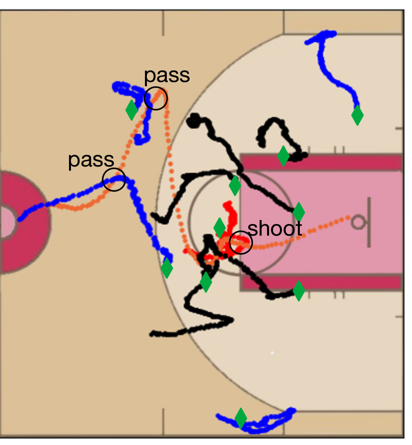
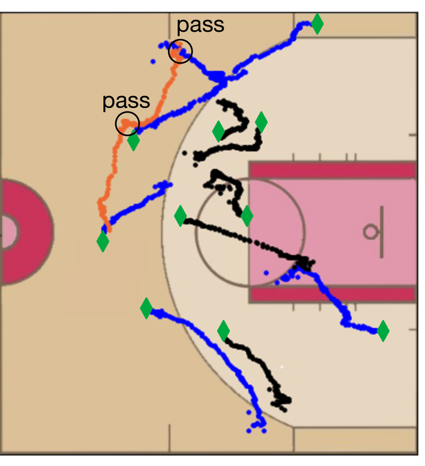
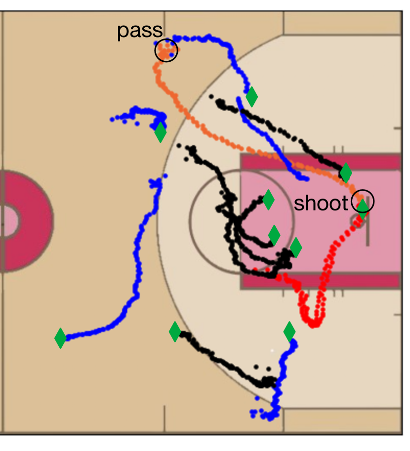
We now perform a case study to qualitatively demonstrate the practicability of value-guided conditional generation. Figure 3 shows three cases, all of which are sampled from the trajectories generated by PlayBest. In Figure 3(a), we visualize a possession generated with a high reward. The players in the blue team share the ball well and managed to find the red player near the free-throw line. At the time the red player shoots the ball, no defender is between him and the basket. The outcome of this simulated play is a 2-point basket. In Figures 3(b) and 3(c), two different plans with the same horizon are generated by PlayBest given the same initial player and ball positions. In Figure 3(b), we observe a more conservative strategy where the ball is repeatedly passed between the blue players near the perimeter, which is also valued with a lower reward. In spite of the same initial conditions, PlayBest generates a more aggressive strategy in Figure 3(c) in that the ball is passed directly to the low post that leads to a 2-point basket, suggesting an aggressive tactic execution. These cases illustrate that PlayBest is able to not only synthesize realistic trajectories but also output high-reward and diverse trajectories for planning multi-agent tactics as well as for enhancing decision-making. Additional experimental results are detailed in Appendix A.3.

5 Related Work

Reinforcement Learning for Planning. Reinforcement learning is a learning-based control approach. A wide range of application domains have seen remarkable achievements through the use of reinforcement learning algorithms, such as robotics (Kalashnikov et al., 2018a), autonomous vehicles (Balaji et al., 2019), industrial regulation (Gasparik et al., 2018), financial sectors (Meng & Khushi, 2019), healthcare (Yu et al., 2019), news suggestions (Zheng et al., 2018), gaming (Silver et al., 2017), and marketing (Jin et al., 2018). Despite its wide use, many RL applications depend on an online environment that facilitates interactions. In numerous circumstances, acquiring data online is either expensive, unethical, or dangerous, making it a luxury. Consequently, it is preferable to learn effective behavior strategies using only pre-existing data. Offline RL has been suggested to fully utilize previously gathered data without the need for environmental interaction (Fujimoto et al., 2019; Agarwal et al., 2020; Kumar et al., 2020; Levine et al., 2020; Fu et al., 2020), which has found applications in areas such as dialogue systems (Jaques et al., 2019), robotic manipulation techniques (Kalashnikov et al., 2018b), and navigation (Kahn et al., 2021).

Sports & Machine Learning. Machine learning and AI have recently been employed in sports analytics to comprehend and advise human decision-making (Aoki et al., 2017; Ruiz et al., 2017; Decroos et al., 2018; Sun et al., 2020; Tuyls et al., 2021; Robberechts et al., 2021; Wang et al., 2022a). Luo et al. (2021) suggested a player ranking technique that combines inverse RL and Q-learning. Wang et al. (2022b) developed a position-aware fusion framework for objectively forecasting stroke returns based on rally progress and player style. Chang et al. (2022) predicted returning strokes and player movements based on previous strokes using a dynamic graph and hierarchical fusion approach. While these methods are effective for producing simulations, they may not fully address the goal of maximizing specific objectives (e.g., winning games).

Previous basketball analytics mainly focused on employing recurrent neural networks to analyze player-tracking data for offensive tactics identification and player movement prediction  (McIntyre et al., 2016; Wang & Zemel, 2016; Tian et al., 2020; Terner & Franks, 2020). However, these methods lack labeled interactions between the learning agent and the environment, limiting their ability to uncover optimal decision sequences. Wang et al. (2018) explored the use of RL to improve defensive team decisions, especially the execution of a "double team" strategy. Liu & Hodgins (2018) designed a method using motion capture data to learn robust basketball dribbling maneuvers by training on both locomotion and arm control, achieving robust performance in various scenarios.

6 Conclusion

In this paper, we introduce PlayBest, the diffusion model with conditional sampling in planning optimal basketball trajectories and synthesizing adaptive play strategies.

With the extension of multi-agent environmental dynamics into the diffusion model and fine-grained rewards for the value function, PlayBest has shown impressive capabilities in capturing the intricate dynamics of basketball games and generating play strategies that are consistent with or even surpass professional tactics. Its adaptive nature has allowed for swift adjustments to evolving conditions and facilitated real-time identification of optimal solutions. Extensive simulation studies and analysis of real-world NBA data have confirmed the advantages of PlayBest over traditional planning methods. The generated trajectories and play strategies not only outperform conventional techniques but also exhibit a high level of alignment with professional basketball tactics.

Limitation: Currently we only consider the player movement and only conduct offline evaluation since no online environment for our application is available. Future work will explore the integration of additional sources of information, such as player fatigue and skill levels, into our framework to further enhance its performance. Moreover, we plan to extend the application of PlayBest to other team sports/e-sports, investigating its efficacy in generating adaptive play strategies and trajectories in various dynamic and uncertain environments. Finally, we plan to develop an open environment and a set of benchmarks to not only facilitate research on machine learning for sports but also extend to other real-time dynamic systems.

Appendix A Appendix

A.1 Guided Sampling Algorithm

We summarize the entire procedure of the reward-guided planning of PlayBest in Algorithm 1.

Algorithm 1 Reward Guided Planning

1:  Require diffusion model $\mu_{\theta}$, guide $\mathcal{J}_{\phi}$, scale $\alpha$, covariances $\Sigma^{i}$

2:  while not done do

3:     Acquire state $\mathbf{s}$; initialize trajectory $\bm{\tau}^{N}\sim\mathcal{N}(\bm{0},\bm{I})$

4:     // for the $N$ diffusion steps

5:     for $i=N,\ldots,1$ do

6:        // estimate the mean from the previous diffusion step

7:        $\mu\leftarrow\mu_{\theta}(\bm{\tau}^{i})$

8:        // guide using gradients of return

9:        $\bm{\tau}^{i-1}\sim\mathcal{N}(\mu+\alpha\Sigma\nabla\mathcal{J}(\mu),\Sigma^{i})$

10:        // conditioned on the first given state

11:        $\bm{\tau}^{i-1}_{{\bm{s}}_{0}}\leftarrow{\bm{s}}$   

12:     end for

13:     Execute first action of trajectory $\bm{\tau}^{0}_{\mathbf{a}_{0}}$

14:  end while

A.2 Implementation Details of PlayBest.

We set the planning horizon length to $1,024$ so that all trajectories in the training data can be fitted in our diffusion model. The diffusion step is set to $20$ in all experiments. The learning rate is $2\times 10^{-5}$ without learning rate scheduling. The hidden dimension is set following Janner et al. (2022). The training batch size is set to $512$. We train all models for $245K$ training steps. The value function is optimized with the mean square error loss. The reported results are given by the best-performing checkpoint on the development sets. All experiments are run on the NVIDIA Tesla V100 Tensor Core GPUs with 16GB memory. The code for PlayBest is included in the supplemental materials.

A.3 Additional Experimental Results

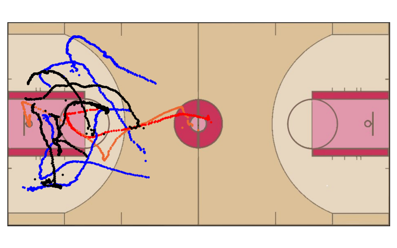
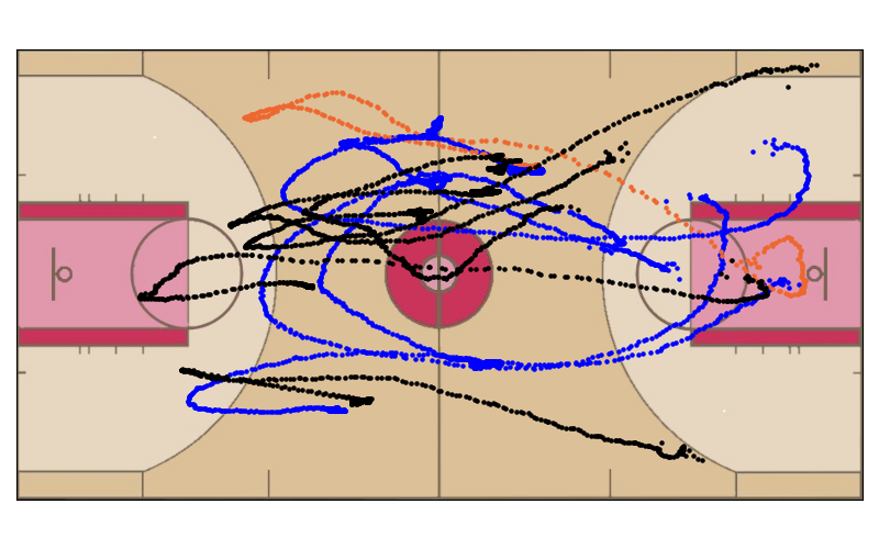
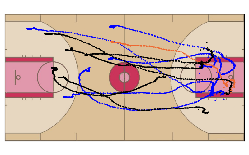
In this section, we provide additional experimental results. For our case studies, we analyze the dynamics of high-reward and low-reward trajectories. In addition to the figures in this section, we have also included the animated files in a .gif format in the supplemental materials.

High-reward trajectories. We sample various scenarios of gameplay where significant points were scored and break down the sequence of actions leading up to these outcomes. The analysis includes three sub-categories:

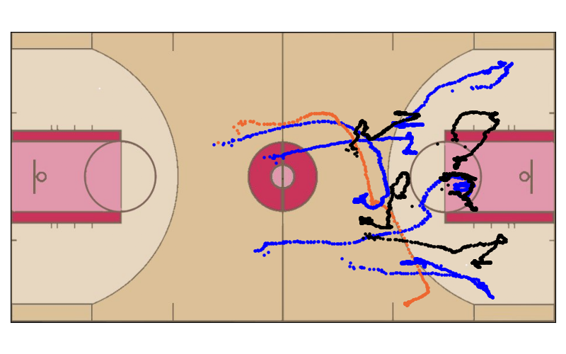
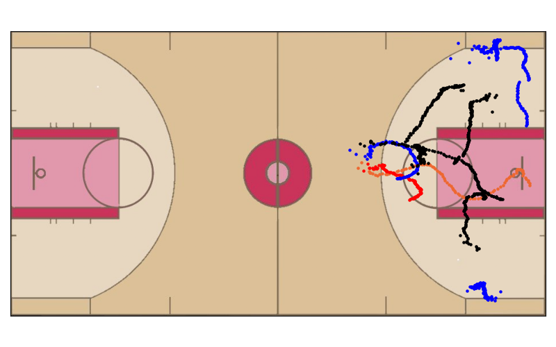
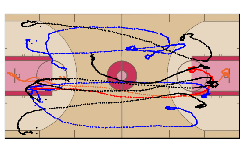
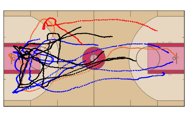
• Effective Passing: We investigate how well-executed passes among players help in penetrating the defense and setting up successful scoring opportunities. In Figure 4(a), we observe good offense by the home team to pass to an open player (No shot occurs in this play). In Figure 4(d), the home team starts in the backcourt getting ready to move into an offensive position. As they move down the court, they appear to make a pass that gets deflected by the defense. The home team still recovers the deflection and then makes a pass to an open 3-point shot. The home team makes the shot. These cases display PlayBest’s ability to find good plays demonstrating effective passing.

• Diverse scoring types: We also analyze instances of different scoring types, including lay-ups and jump shots. In Figure 4(b), the home team takes a run-up shot and makes the shot. In Figure 4(e), the home team starts on offense with a player dribbling down the court. After some time, the player finds an open lane and drives to the basket making a layup using the backboard.

• Rebounds: As aforementioned, we assign a positive reward to encourage rebounding. We will highlight cases where a good rebound leads to immediate scoring opportunities or regaining possession from the opponents. In figure 4(c), the home team obtains a defensive rebound and scores on a fastbreak layup. In Figure 4(f), the away team starts with the ball moving into an offensive position. The home team allows a pass into the key but because of good defense, the away team misses the shot and the home team grabs the rebound, getting ready to move into an offensive position. This displays PlayBest ’s ability to generate nice transition plays from defense to offense.

(a) Reward = $0.368$

(b) Reward = $1.628$

(c) Reward = $3.032$.

(d) Reward = $1.220$.

(e) Reward = $2.647$

(f) Reward = $1.688$

Figure 4: (a, b, c, d, e, f): High-reward possessions generated by PlayBest. The blue team is the home team for whom the rewards are generated, while the black team is the away team. The ball is marked in orange. The player who scores for the blue team is highlighted in Red.

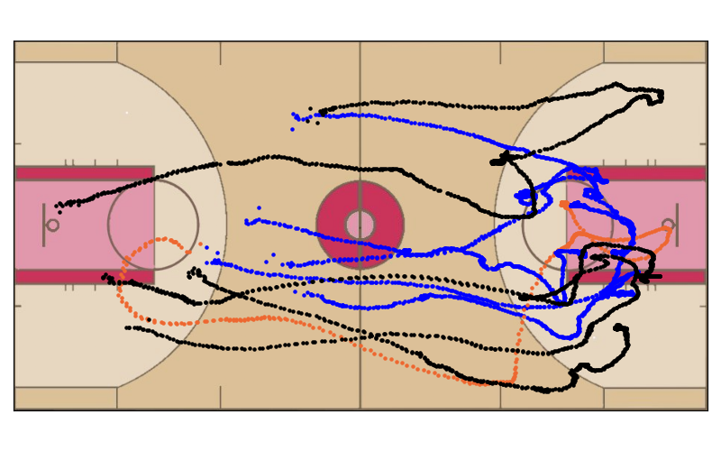
Low-reward trajectories. We further look into trajectories that lead to turnovers - sequences resulting in loss of possession without scoring. Note that some rewards may be negative because later on in the trajectory, the blue team may have played bad basketball and the output of the value function reflects that.

In Figure 5(a), the away team misses a shot, and the home team gets a defensive rebound. However, the home team turns the ball over due to good defense by the away team. In Figure 5(b), the home team gets a defensive rebound and begins moving into the offensive position. PlayBest recognizes that away team defense is in a good position at the end of the frame and thus rates negative. In Figure 5(c), the away team is on offense and turns the ball over. The home team gets the steal but then makes a bad pass when the frame stops.

(a) Reward = $-1.224$.

(b) Reward = $-1.506$

(c) Reward = $-0.557$

Figure 5: (a, b, c): Negative-reward possessions generated by PlayBest. The color scheme is the same as in Figure 4.

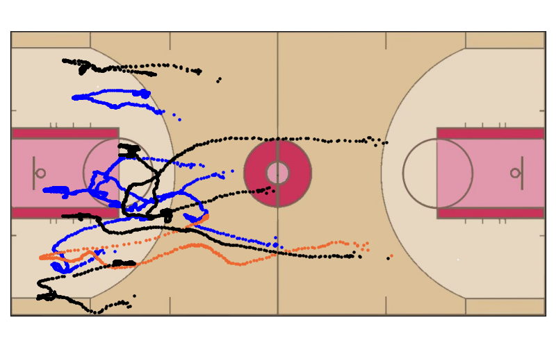
The effect of $\alpha$.

We also focus on the analysis of synthesized trajectories under variable conditions. To highlight the effect of the scaling factor on the decision-making process, we consider trajectories initiated from the same state but with different scaling factors, specifically $\alpha$ values of $0.1$, $1.0$, and $10.0$. By visualizing these trajectories, we aim to demonstrate how variations in the scaling factor can significantly influence the progression and outcomes of the game, further emphasizing the crucial role of this parameter in our model.

(a) $\alpha=0.1$

(b) $\alpha=1.0$

(c) $\alpha=10.0$

Figure 6: (a, b, c): Possessions generated by PlayBest with different $\alpha$.

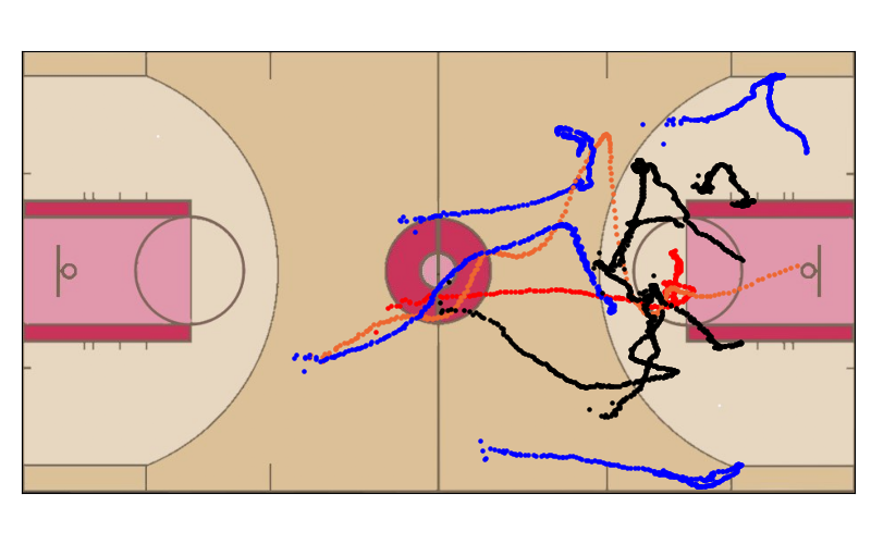
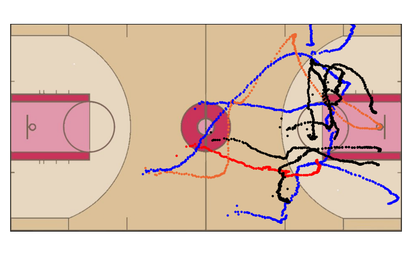
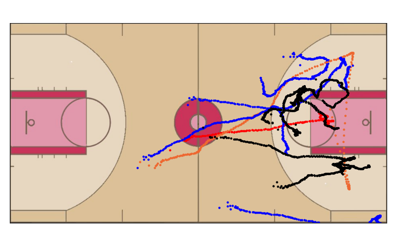
As mentioned in Section 4.3, the increase of $\alpha$ leads to higher overall cumulative rewards on the test games. Then the question is, why not keep increasing the value of $\alpha$? To provide a deeper insight into this, we conduct a comparative study demonstrated in Figure 6. When $\alpha=1.0$, there seems to be a mysterious force that pulls the ball to the basket. In the $\alpha=10.0$ case, the synthesized trajectory becomes even less interpretable since the ball never goes through the basket. In both $\alpha=1.0$ and $\alpha=10.0$ cases, the ball exhibits behaviors that defy the laws of physics, seemingly being propelled towards the basket as if being controlled by an invisible player.

References

- pbp (2016) Play-by-play data, 2016. URL https://www.bigdataball.com/datasets/nba/.
- spo (2016) Sportvu data, 2016. URL https://github.com/rajshah4/BasketballData/tree/master/2016.NBA.Raw.SportVU.Game.Logs.
- Agarwal et al. (2020) Agarwal, R., Schuurmans, D., and Norouzi, M. An optimistic perspective on offline reinforcement learning. In International Conference on Machine Learning, pp. 104–114. PMLR, 2020.
- Ajay et al. (2022) Ajay, A., Du, Y., Gupta, A., Tenenbaum, J., Jaakkola, T., and Agrawal, P. Is conditional generative modeling all you need for decision-making? arXiv preprint arXiv:2211.15657, 2022.
- Aoki et al. (2017) Aoki, R. Y., Assuncao, R. M., and Vaz de Melo, P. O. Luck is hard to beat: The difficulty of sports prediction. In KDD, pp. 1367–1376, 2017.
- Balaji et al. (2019) Balaji, B., Mallya, S., Genc, S., Gupta, S., Dirac, L., Khare, V., Roy, G., Sun, T., Tao, Y., Townsend, B., et al. Deepracer: Educational autonomous racing platform for experimentation with sim2real reinforcement learning. arXiv preprint arXiv:1911.01562, 2019.
- Botev et al. (2013) Botev, Z. I., Kroese, D. P., Rubinstein, R. Y., and L’Ecuyer, P. The cross-entropy method for optimization. In Handbook of statistics, volume 31, pp. 35–59. Elsevier, 2013.
- Chang et al. (2022) Chang, K.-S., Wang, W.-Y., and Peng, W.-C. Where will players move next? dynamic graphs and hierarchical fusion for movement forecasting in badminton. arXiv preprint arXiv:2211.12217, 2022.
- Chen et al. (2022) Chen, X., Jiang, J., Jin, K., Zhou, Y., Liu, M., Brantingham, P. J., and Wang, W. Reliable: Offline reinforcement learning for tactical strategies in professional basketball games. In CIKM, pp. 3023–3032. ACM, 2022.
- Chua et al. (2018) Chua, K., Calandra, R., McAllister, R., and Levine, S. Deep reinforcement learning in a handful of trials using probabilistic dynamics models. Advances in neural information processing systems, 31, 2018.
- Decroos et al. (2018) Decroos, T., Van Haaren, J., and Davis, J. Automatic discovery of tactics in spatio-temporal soccer match data. In KDD, pp. 223–232, 2018.
- Fu et al. (2020) Fu, J., Kumar, A., Nachum, O., Tucker, G., and Levine, S. D4rl: Datasets for deep data-driven reinforcement learning. arXiv preprint arXiv:2004.07219, 2020.
- Fujimoto et al. (2019) Fujimoto, S., Meger, D., and Precup, D. Off-policy deep reinforcement learning without exploration. In International conference on machine learning, pp. 2052–2062. PMLR, 2019.
- Gasparik et al. (2018) Gasparik, A., Gamble, C., and Gao, J. Safety-first ai for autonomous data centre cooling and industrial control. DeepMind Blog, 2018.
- Ho et al. (2020) Ho, J., Jain, A., and Abbeel, P. Denoising diffusion probabilistic models. Advances in Neural Information Processing Systems, 33:6840–6851, 2020.
- Janner et al. (2022) Janner, M., Du, Y., Tenenbaum, J. B., and Levine, S. Planning with diffusion for flexible behavior synthesis. arXiv preprint arXiv:2205.09991, 2022.
- Jaques et al. (2019) Jaques, N., Ghandeharioun, A., Shen, J. H., Ferguson, C., Lapedriza, A., Jones, N., Gu, S., and Picard, R. Way off-policy batch deep reinforcement learning of implicit human preferences in dialog. arXiv preprint arXiv:1907.00456, 2019.
- Jin et al. (2018) Jin, J., Song, C., Li, H., Gai, K., Wang, J., and Zhang, W. Real-time bidding with multi-agent reinforcement learning in display advertising. In CIKM, pp. 2193–2201, 2018.
- Kahn et al. (2021) Kahn, G., Abbeel, P., and Levine, S. Badgr: An autonomous self-supervised learning-based navigation system. IEEE Robotics and Automation Letters, 6(2):1312–1319, 2021.
- Kalashnikov et al. (2018a) Kalashnikov, D., Irpan, A., Pastor, P., Ibarz, J., Herzog, A., Jang, E., Quillen, D., Holly, E., Kalakrishnan, M., Vanhoucke, V., et al. Qt-opt: Scalable deep reinforcement learning for vision-based robotic manipulation. arXiv preprint arXiv:1806.10293, 2018a.
- Kalashnikov et al. (2018b) Kalashnikov, D., Irpan, A., Pastor, P., Ibarz, J., Herzog, A., Jang, E., Quillen, D., Holly, E., Kalakrishnan, M., Vanhoucke, V., et al. Scalable deep reinforcement learning for vision-based robotic manipulation. In ICRL, pp. 651–673, 2018b.
- Ke et al. (2019) Ke, N. R., Singh, A., Touati, A., Goyal, A., Bengio, Y., Parikh, D., and Batra, D. Modeling the long term future in model-based reinforcement learning. In International Conference on Learning Representations, 2019.
- Kostrikov et al. (2021) Kostrikov, I., Nair, A., and Levine, S. Offline reinforcement learning with implicit q-learning. arXiv preprint arXiv:2110.06169, 2021.
- Kumar et al. (2020) Kumar, A., Zhou, A., Tucker, G., and Levine, S. Conservative q-learning for offline reinforcement learning. Advances in Neural Information Processing Systems, 33:1179–1191, 2020.
- Levine et al. (2020) Levine, S., Kumar, A., Tucker, G., and Fu, J. Offline reinforcement learning: Tutorial, review, and perspectives on open problems. arXiv preprint arXiv:2005.01643, 2020.
- Liu & Hodgins (2018) Liu, L. and Hodgins, J. Learning basketball dribbling skills using trajectory optimization and deep reinforcement learning. TOG, 37(4):1–14, 2018.
- Luo et al. (2021) Luo, Y., Schulte, O., and Poupart, P. Inverse reinforcement learning for team sports: valuing actions and players. In IJCAI, pp. 3356–3363, 2021.
- McIntyre et al. (2016) McIntyre, A., Brooks, J., Guttag, J., and Wiens, J. Recognizing and analyzing ball screen defense in the nba. In Proc. of the MIT Sloan Sports Analytics Conference, pp. 11–12, 2016.
- Meng & Khushi (2019) Meng, T. L. and Khushi, M. Reinforcement learning in financial markets. Data, 4(3):110, 2019.
- Nagabandi et al. (2018) Nagabandi, A., Kahn, G., Fearing, R. S., and Levine, S. Neural network dynamics for model-based deep reinforcement learning with model-free fine-tuning. In 2018 IEEE international conference on robotics and automation (ICRA), pp. 7559–7566. IEEE, 2018.
- Robberechts et al. (2021) Robberechts, P., Van Haaren, J., and Davis, J. A bayesian approach to in-game win probability in soccer. In KDD, pp. 3512–3521, 2021.
- Ronneberger et al. (2015) Ronneberger, O., Fischer, P., and Brox, T. U-net: Convolutional networks for biomedical image segmentation. In Medical Image Computing and Computer-Assisted Intervention–MICCAI 2015: 18th International Conference, Munich, Germany, October 5-9, 2015, Proceedings, Part III 18, pp. 234–241. Springer, 2015.
- Ruiz et al. (2017) Ruiz, H., Power, P., Wei, X., and Lucey, P. " the leicester city fairytale?" utilizing new soccer analytics tools to compare performance in the 15/16 & 16/17 epl seasons. In KDD, pp. 1991–2000, 2017.
- Silver et al. (2017) Silver, D., Schrittwieser, J., Simonyan, K., Antonoglou, I., Huang, A., Guez, A., Hubert, T., Baker, L., Lai, M., Bolton, A., et al. Mastering the game of go without human knowledge. Nature, 550(7676):354–359, 2017.
- Sohl-Dickstein et al. (2015) Sohl-Dickstein, J., Weiss, E., Maheswaranathan, N., and Ganguli, S. Deep unsupervised learning using nonequilibrium thermodynamics. In International Conference on Machine Learning, pp. 2256–2265. PMLR, 2015.
- Sun et al. (2020) Sun, X., Davis, J., Schulte, O., and Liu, G. Cracking the black box: Distilling deep sports analytics. In KDD, pp. 3154–3162, 2020.
- Talvitie (2014) Talvitie, E. Model regularization for stable sample rollouts. In UAI, pp. 780–789, 2014.
- Tassa et al. (2012) Tassa, Y., Erez, T., and Todorov, E. Synthesis and stabilization of complex behaviors through online trajectory optimization. In 2012 IEEE/RSJ International Conference on Intelligent Robots and Systems, pp. 4906–4913. IEEE, 2012.
- Terner & Franks (2020) Terner, Z. and Franks, A. Modeling player and team performance in basketball. Annual Review of Statistics and Its Application, 8, 2020.
- Tian et al. (2020) Tian, C., De Silva, V., Caine, M., and Swanson, S. Use of machine learning to automate the identification of basketball strategies using whole team player tracking data. Applied Sciences, 10(1):24, 2020.
- Tuyls et al. (2021) Tuyls, K., Omidshafiei, S., Muller, P., Wang, Z., Connor, J., Hennes, D., Graham, I., Spearman, W., Waskett, T., Steel, D., et al. Game plan: What ai can do for football, and what football can do for ai. JAIR, 71:41–88, 2021.
- Wang et al. (2018) Wang, J., Fox, I., Skaza, J., Linck, N., Singh, S., and Wiens, J. The advantage of doubling: A deep reinforcement learning approach to studying the double team in the nba. arXiv preprint arXiv:1803.02940, 2018.
- Wang & Zemel (2016) Wang, K.-C. and Zemel, R. Classifying nba offensive plays using neural networks. In Proc. of MIT Sloan Sports Analytics Conference, volume 4, 2016.
- Wang et al. (2019) Wang, T., Bao, X., Clavera, I., Hoang, J., Wen, Y., Langlois, E., Zhang, S., Zhang, G., Abbeel, P., and Ba, J. Benchmarking model-based reinforcement learning. arXiv preprint arXiv:1907.02057, 2019.
- Wang et al. (2022a) Wang, W.-Y., Chan, T.-F., Peng, W.-C., Yang, H.-K., Wang, C.-C., and Fan, Y.-C. How is the stroke? inferring shot influence in badminton matches via long short-term dependencies. ACM Transactions on Intelligent Systems and Technology, 14(1):1–22, 2022a.
- Wang et al. (2022b) Wang, W.-Y., Shuai, H.-H., Chang, K.-S., and Peng, W.-C. Shuttlenet: Position-aware fusion of rally progress and player styles for stroke forecasting in badminton. In Proceedings of the AAAI Conference on Artificial Intelligence, volume 36, pp. 4219–4227, 2022b.
- Witkin & Kass (1988) Witkin, A. and Kass, M. Spacetime constraints. ACM Siggraph Computer Graphics, 22(4):159–168, 1988.
- Yanai et al. (2022) Yanai, C., Solomon, A., Katz, G., Shapira, B., and Rokach, L. Q-ball: Modeling basketball games using deep reinforcement learning. In AAAI, pp. 8806–8813. AAAI Press, 2022.
- Yu et al. (2019) Yu, C., Liu, J., and Nemati, S. Reinforcement learning in healthcare: A survey. arXiv preprint arXiv:1908.08796, 2019.
- Zheng et al. (2018) Zheng, G., Zhang, F., Zheng, Z., Xiang, Y., Yuan, N. J., Xie, X., and Li, Z. Drn: A deep reinforcement learning framework for news recommendation. In WWW, pp. 167–176, 2018.