PILLAR: How to make semi-private learning more effective

Abstract

In Semi-Supervised Semi-Private (SP) learning, the learner has access to both public unlabelled and private labelled data. We propose a computationally efficient algorithm that, under mild assumptions on the data, provably achieves significantly lower private labelled sample complexity and can be efficiently run on real-world datasets. For this purpose, we leverage the features extracted by networks pre-trained on public (labelled or unlabelled) data, whose distribution can significantly differ from the one on which SP learning is performed. To validate its empirical effectiveness, we propose a wide variety of experiments under tight privacy constraints ($\epsilon=0.1$) and with a focus on low-data regimes. In all of these settings, our algorithm exhibits significantly improved performance over available baselines that use similar amounts of public data.

1 Introduction

In recent years, Machine Learning (ML) models have become ubiquitous in our daily lives. It is now common for these models to be trained on vast amounts of sensitive private data provided by users to offer better services tailored to their needs. However, this has given rise to concerns regarding users’ privacy, and recent works (Shokri et al., 2017; Ye et al., 2022; Carlini et al., 2022) have demonstrated that attackers can maliciously query ML models to reveal private information. To address this problem, the de-facto standard remedy is to enforce $(\epsilon,\delta)-$Differential Privacy (DP) guarantees on the ML algorithms (Dwork et al., 2006). However, satisfying these guarantees often comes at the cost of the model’s utility, unless the amount of available private training data is significantly increased (Kasiviswanathan et al., 2011; Blum et al., 2005; Beimel et al., 2013a, b; Feldman and Xiao, 2014). A way to alleviate the utility degradation is to leverage feature extractors pre-trained on a large-scale dataset (assumed to be public) and whose data generating distribution can differ from the one from which the private data is sampled (Tramer and Boneh, 2021; De et al., 2022; Li et al., 2022a; Kurakin et al., 2022). Training a linear classifier on top of these pre-trained features has been shown to be among the most cost-efficient and effective techniques (Tramer and Boneh, 2021; De et al., 2022). Gains in utility can also be obtained if part of the private data is deemed public: a setting known as Semi-Private (SP) learning (Alon et al., 2019; Yu et al., 2021; Li et al., 2022b; Papernot et al., 2017, 2018).

In this work, we propose a SP algorithm to efficiently learn a linear classifier on top of features output by pre-trained neural networks. The idea is to leverage the public data to estimate the Principal Components, and then to project the private dataset on the top-$k$ Principal Components. For the task of learning linear halfspaces, this renders the algorithm’s sample complexity independent of the dimensionality of the data, provided that the data generating distribution satisfies a low rank separability condition, specified in Definition 3. We call this class of distributions large margin low rank distributions. For the practically relevant task of image classification, we show that pre-trained representations satisfy this condition for a wide variety of datasets. In line with concerns raised by the concurrent work of Tramèr et al. (2022), we demonstrate the effectiveness of our algorithm not only on standard image classification benchmarks used in the DP literature (i.e. CIFAR-10 and CIFAR-100) but also on a range of datasets (Figure 1) that we argue better represents the actual challenges of private training.

Indeed, in our evaluations we particularly focus on private data distributions that deviate significantly from the pre-training ones and on low-data regimes. We believe that testing on such relevant benchmarks is essential to demonstrate the practical applicability of our algorithm. Strikingly, we observe that the benefits of our approach increase as the privacy guarantees become tighter, i.e., when $\epsilon$ is lower. In contrast, we find that reducing the dimensionality of the input without imposing privacy guarantees, i.e., when $\epsilon=\infty$, leads to a decline in the model’s performance.

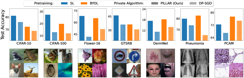
Figure 1: We evaluate our algorithm PILLAR on CIFAR-10, CIFAR-100, GTSRB, Flower-16, Dermnet, Pneumonia, and PCAM. PILLAR  significantly outperforms the strongest DP baseline DP-SGD (Abadi et al., 2016; Li et al., 2022c) (see Section 4.1 for comparison with other baselines). Both methods use features extracted from a ResNet-50 pre-trained on ImageNet-1K using either Supervised Learning (SL) or Self-Supervised Learning (BYOL (Grill et al., 2020))

To summarise, our contributions are the following:

• We propose an SP algorithm, PILLAR, that improves classification accuracy over existing baselines. Our algorithm, as well as baselines, use representations generated by pre-trained feature extractors. We demonstrate that our improvements are independent of the chosen pre-training strategy.

• We prove that, for learning half-spaces, our algorithm achieves dimension-independent private labelled sample complexity for large margin low rank distributions.

• We improve DP and SP evaluation benchmarks for image classification by focusing on private datasets that differ significantly from pre-training datasets (e.g. ImageNet-1K (Deng et al., 2009)) and with small amounts training data available. We enforce strict privacy constraints to better represent real-world challenges, and show our algorithm is extremely effective in these challenging settings.

2 Semi-Private Learning

We begin by defining Differential Privacy (DP). DP ensures that the output distribution of a randomized algorithm remains stable when a single data point is modified. In this paper, a differentially private learning algorithm produces comparable distributions over classifiers when trained on neighbouring datasets. Neighbouring datasets refer to datasets that differ by a single entry. Formally,

Definition 1 (Differential Privacy Dwork et al. (2006)).

A learning algorithm ${\mathcal{A}}$ is $(\epsilon,\delta)$-differential private, if for any two datasets $S,S^{\prime}$ differing in one entry and for all outputs ${\mathcal{Z}}$, we have,

$${\mathbb{P}}\left[{{\mathcal{A}}(S)\in{\mathcal{Z}}}\right]\leq e^{\epsilon}{\mathbb{P}}\left[{{\mathcal{A}}(S)\in{\mathcal{Z}}}\right]+\delta.$$

For $\epsilon<1$ and $\delta=o\left({1/n}\right)$, $(\epsilon,\delta)$-differential privacy provides valid protection against potential privacy attacks (Carlini et al., 2022).

Differential Privacy and Curse of Dimensionality

Similar to non-private learning, the most common approach to DP learning is through Differentially Private Empirical Risk Minimization (DP-ERM), with the most popular optimization procedure being DP-SGD (Abadi et al., 2016) or analogous DP-variants of typical optimization algorithms. However, unlike non-private ERM, the sample complexity of DP-ERM suffers from a linear dependence on the dimensionality of the problem (Chaudhuri et al., 2011; Bassily et al., 2014a). Hence, we explore slight relaxations to this definition of privacy to alleviate this problem. We show theoretically (Section 3) and through extensive experiments (Section 4 and 5) that this is indeed possible with some realistic assumptions on the data and a slightly relaxed definition of privacy known as semi-private learning that we describe below. For a discussion of broader impacts and limitations, please refer to Appendix C.

2.1 Semi-Private Learning

The concept of semi-private learner was introduced in Alon et al. (2019). In this setting, the learning algorithm is assumed to have access to both a private labelled and a public (labelled or unlabelled) dataset. In this work, we assume the case of only having an unlabelled public dataset. This specific setting has been referred to as Semi-Supervised Semi-Private learning in Alon et al. (2019). However, for the sake of brevity, we will refer to it as Semi-Private learning (SPL).

Definition 2 ($(\alpha,\beta,\epsilon,\delta)$-semi-private learner on a family of distributions ${\mathcal{D}}$).

An algorithm ${\mathcal{A}}$ is said to $(\alpha,\beta,\epsilon,\delta)$-semi-privately learn a hypothesis class ${\mathcal{H}}$ on a family of distributions ${\mathcal{D}}$, if for any distribution $D\in{\mathcal{D}}$, given a private labelled dataset $S^{L}$ of size $n^{L}$ and a public unlabelled dataset $S^{U}$ of size $n^{U}$ sampled i.i.d. from $D$, ${\mathcal{A}}$ is $(\epsilon,\delta)$-DP with respect to $S^{L}$ and outputs a hypothesis $\hat{h}$ satisfying

$${\mathbb{P}}[{\mathbb{P}}_{(x,y)\sim D}\left[{h(x)\neq y}\right]\leq\alpha]\geq 1-\beta,$$

where the outer probability is over the randomness of $S^{L},S^{U},$ and ${\mathcal{A}}$.

Further, the sample complexity $n^{L}$ and $n^{U}$ must be polynomial in $\frac{1}{\alpha},\frac{1}{\beta},$ and the size of the input space. In addition, $n^{L}$ must also be polynomial in $\frac{1}{\epsilon}$ and $\frac{1}{\delta}$. The algorithm is said to be efficient if it also runs in time polynomial in $\frac{1}{\alpha},\frac{1}{\beta},$ and the size of the input domain.

A key distinction between our work and the previous study by Alon et al. (2019) is that they examine the distribution-independent agnostic learning setting, whereas we investigate the distribution-specific realisable setting. On the other hand, while their algorithm is computationally inefficient, ours can be run in time polynomial in the relevant parameters and implemented in practice on various datasets with state-of-the-art results. We discuss our algorithm in Section 2.2.

Relevance of Semi-Private Learning

In various privacy-sensitive domains such as healthcare, legal, social security, and census data, there is often some amounts of publicly available data in addition to the private data. For instance, the U.S. Census Bureau office has partially released historical data before 2020 without enforcing any differential privacy guarantees . It has also been observed that different data providers may have varying levels of concerns about privacy (Jensen et al., 2005). In medical data, some patients may consent to render some of their data public to foster research. In other cases, data may become public due to the expiration of the right to privacy after specific time limits .

It is also very likely that this public data may be unlabelled for the task at hand. For example, if data is collected to train a model to predict a certain disease, the true diagnosis may have been intentionally removed from the available public data to protect sensitive information of the patients. Further, the data may had been collected for a different purpose like a vaccine trial. Finally, the cost of labelling may be prohibitive in some cases. Hence, when public (unlabelled) data is already available, we focus on harnessing this additional data effectively, while safeguarding the privacy of the remaining private data. We hope this can lead to the development of highly performant algorithms which in turn can foster wider adoption of privacy-preserving techniques.

2.2 PILLAR: An Efficient Semi-Private Learner

Algorithm 1 PILLAR: ${\mathcal{A}}_{\epsilon,\delta}\left({k,\zeta}\right)$

1:Input: Labelled dataset $S^{L}$, Unlabelled dataset $S^{U}$, low-dimension $k$, distributional parameter $\zeta$, high probability parameter $\beta$.

2:Using $S^{U}$, construct $\widehat{\Sigma}=\sum_{x\in S^{U}}xx^{\top}/n^{U}$.

3:Construct the transformation matrix $\hat{A}_{k}$ whose $i^{\it th}$ column is the $i^{\it th}$ eigenvector of $\widehat{\Sigma}$.

4:Project $S^{L}$ with the transformation matrix $\hat{A}_{k}$,

$$S^{L}_{k}=\{(\hat{A}_{k}^{\top}x,y):(x,y)\in S^{L}\}.$$

5:Obtain $v_{k}={\mathcal{A}}_{\mathrm{Noisy-SGD}}(S^{L}_{k},\ell,(\epsilon,\delta),\nicefrac{{\beta}}{{4}})$ where $\ell$ is a $\frac{1}{\zeta}$-Lipschitz loss function defined as

$$\ell(w,(x,y))=\max\left\{1-\frac{y}{\zeta}\left\langle{w,x}\right\rangle,0\right\}.$$ (1)

6:Output: Return $\hat{w}=\hat{A}_{k}v_{k}$.

Figure 2: Left: Diagram describing how PILLAR is applied in image classification (using DP-SGD with cross-entropy loss in Line 4 of Algorithm 1). Right: PILLAR for learning linear halfspaces.

In this work, we propose a (semi-supervised) semi-private learning algorithm called PILLAR (PrIvate Learning with Low rAnk Representations), described in Figure 2. Before providing formal guarantees in Section 3, we first describe how PILLAR is applied in practice. Our algorithm works in two stages.

Leveraging recent practices (De et al., 2022; Tramer and Boneh, 2021) in DP training with deep neural networks, we first use pre-trained feature extractors to transform the private labelled and public unlabelled datasets to the representation space to obtain the private and public representations. We use the representations in the penultimate layer of the pre-trained neural network for this purpose. As shown in Figure 2, the feature extractor is trained on large amounts of labelled or unlabelled public data, following whatever training procedure is deemed most suitable. For this paper, we pre-train a ResNet-50 using supervised training (SL), self-supervised training (BYOL (Grill et al., 2020) and MocoV2+ (Chen et al., 2020)), and semi-supervised training (SemiSL and Semi-WeakSL (Yalniz et al., 2019)) on ImageNet. In the main body, we only focus on SL and BYOL pre-training. As we discuss extensively in Section B.6, our algorithm is effective independent of the choice of the pre-training algorithm. In addition, while the private and public datasets are required to be from the same (or similar) distribution, we show that the pre-training dataset can come from a significantly different distribution. In fact, we use ImageNet as the pre-training dataset for all our experiments even when the distributions of the public and private datasets range from CIFAR-10/100 to histological and x-ray images as shown in Figure 1. Recently, Gu et al. (2023) have explored the complementary question of how to choose the right pre-training dataset.

In the second stage, PILLAR takes as input the feature representations of the private labelled and public unlabelled datasets, and feeds them to Algorithm 1. We denote these datasets of representations as $S^{L}$ and $S^{U}$ respectively. Briefly,  Algorithm 1 projects the private dataset $S^{L}$ onto a low-dimensional space spanned by the top principal components estimated with $S^{U}$, and then applies gradient-based private algorithms (e.g. Noisy-SGD (Bassily et al., 2014a)) to learn a linear classifier on top of the projected features. Algorithm 1 provides an implementation of PILLAR with Noisy-SGD, whereas in our experiments we show that commonly used DP-SGD (Abadi et al., 2016) is also effective.

3 Theoretical Results

In this section, we first describe the assumptions under which we provide our theoretical results and show they can be motivated both empirically and theoretically. Then, we show a dimension-independent sample complexity bound for PILLAR under the mentioned assumptions.

3.1 Problem setting

Our theoretical analysis focuses on learning linear halfspaces $\mathcal{H}_{L}^{d}$ in $d$ dimensions. Consider the instance space ${\mathcal{X}}_{d}=B_{2}^{d}=\left\{{x\in{\mathbb{R}}^{d}:\left\lVert x\right\rVert_{2}=1}\right\}$ as the $d$-dimensional unit sphere and the binary label space ${\mathcal{Y}}=\left\{{-1,1}\right\}$. In practice, the instance space is the (normalized) representation space obtained from the pre-trained network. The hypothesis class of linear halfspaces is

$$\mathcal{H}_{L}^{d}=\left\{{f_{w}(x)=\text{sign}\left({\left\langle{w,x}\right\rangle}\right)|w\in B_{2}^{d}}\right\}.$$

We consider the setting of distribution-specific learning, where our family of distributions admits a large margin linear classifier that contains a significant projection on the top principal components of the population covariance matrix. We formalise this as $\left({\gamma,\xi_{k}}\right)$-Large margin low rank distributions.

Definition 3 ($\left({\gamma,\xi_{k}}\right)$-Large margin low rank distribution).

A distribution $D$ over ${\mathcal{X}}_{d}\times{\mathcal{Y}}$ is a $\left({\gamma,\xi_{k}}\right)$-Large margin low rank distribution if there exists $w^{\star}\in B_{2}^{d}$ such that

• ${\mathbb{P}}_{(x,y)\sim D}\left[{\frac{y\left\langle{w^{\star},x}\right\rangle}{\left\lVert w^{\star}\right\rVert_{2}\left\lVert x\right\rVert_{2}}\geq\gamma}\right]=1$   (Large-margin),

• $\left\lVert A_{k}A_{k}^{\top}w^{\star}\right\rVert_{2}\geq 1-\xi_{k}$  (Low-rank separability).

where $A_{k}$ is a $d\times k$ matrix whose columns are the top $k$ eigenvectors of ${\mathbb{E}}_{X\sim D_{X}}\left[{X^{\top}X}\right]$.

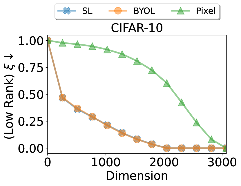
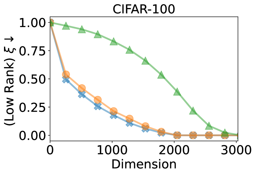
Figure 3: Estimate of $\xi$ for linear classifiers trained on embeddings of two CIFAR-10 and CIFAR-100 classes, extracted from pre-trained ResNet50s, as well as the raw images (Pixel).

It is worth noting that for every distribution that admits a positive margin $\gamma$, the low-rank separability condition is automatically satisfied for all $k\leq d$ with some $\xi_{k}\geq 0$. However, the low rank separability is helpful for learning, only if it holds for a small $k$ and small $\xi_{k}$ simultaneously. These assumptions are both theoretically and empirically realisable. Theoretically, we show in Example 1 that a class of commonly studied Gaussian mixture distributions satisfies these properties. Empirically, we show in Figure 3 that pre-trained features satisfy these properties with small $\xi$ and $k$.

Example 1.

A distribution $D$ over ${\mathcal{X}}\times{\mathcal{Y}}$ is a $(\theta,\sigma^{2})$-Large margin Gaussian mixture distribution if there exists $w^{\star},\mu\in B_{2}^{d}$, such that $\left\langle{\mu,w^{\star}}\right\rangle=0$, the conditional random variable $X|y$ is distributed according to a normal distribution with mean $\mu y$ and covariance matrix $\theta w^{\star}\left({w^{\star}}\right)^{\top}+\sigma^{2}I_{d}$ and $y\in\{-1,1\}$ is distributed uniformly.

For any $\theta,\sigma^{2}=O(\nicefrac{{1}}{{\sqrt{d}}})$, it is easy to see that this family of distributions satisfies the large margin low rank properties in Definition 3 for $k=2$ and $\xi=0$. Next, we show empirically that these assumptions approximately hold on the features of pre-trained feature extractors we use in this work.

Pre-trained features are almost Large-Margin and Low-Rank

Figure 3 shows that feature representations of CIFAR-10 and CIFAR-100 obtained by various pre-training strategies approximately satisfy the conditions of Definition 3. To verify the low-rank separability assumption, we first train a binary linear SVM $w^{\star}$ for a pair of classes on the representation space and estimate $\xi_{k}=1-\left\lVert A_{k}A_{k}^{\top}w^{\star}\right\rVert_{2}$ as defined in Definition 3. We also compute $\xi_{k}$ when $w^{\star}$ is trained on the pixel space . As shown in Figure 3, images in the representation space are better at satisfying the low-rank separability assumption compared to images in the pixel space.

3.2 Private labelled sample complexity analysis

In this section, we bound the sample complexity of PILLAR for learning linear halfspaces. Our theoretical analysis relies on a scaled hinge loss function that depends on the privacy parameters $\epsilon,\delta$, as well as an additional parameter $\zeta$, characterized by $\gamma$ and $\xi_{k}$. We also denote the gap between the $k^{\mathrm{th}}$ and the ${k+1}^{\mathrm{th}}$ eigenvalue of the population covariance matrix as $\Delta_{k}$.

Theorem 1 shows that if the private and public datasets come from the same large-margin low rank distribution, then PILLAR defined in Algorithm 1 is both $\left({\epsilon,\delta}\right)$-DP with respect to the private dataset as well as accurate, with relatively small number of private labelled data. As motivated in Section 3.1, the feature representations of images are usually from large-margin low rank distributions. Thus, in practical implementation, the private and public datasets refer to private and public representations, as shown in Figure 2.

Theorem 1.

Let $k\leq d\in{\mathbb{N}},\gamma_{0}\in(0,1),$ and $\xi_{0}\in[0,1)$ satisfy $\xi_{0}<1-\nicefrac{{\gamma_{0}}}{{10}}$. Consider the family of distributions ${\mathcal{D}}_{\gamma_{0},\xi_{0}}$ which consists of all $\left({\gamma,\xi_{k}}\right)$-large margin low rank distributions over ${\mathcal{X}}_{d}\times{\mathcal{Y}}$, where $\gamma\geq\gamma_{0}$ and $\xi_{k}\leq\xi_{0}$. For any $\alpha\in\left({0,1}\right),\beta\in\left({0,\nicefrac{{1}}{{4}}}\right)$, $\epsilon\in\left({0,\nicefrac{{1}}{{\sqrt{k}}}}\right)$, and $\delta\in(0,1)$, ${\mathcal{A}}_{\epsilon,\delta}(k,\zeta)$, described by Algorithm 1 is an $(\alpha,\beta,\epsilon,\delta)$-semi-private learner for linear halfspaces $\mathcal{H}_{L}^{d}$ on ${\mathcal{D}}_{\gamma_{0},\xi_{0}}$ with sample complexity

$$n^{U}=O\left(\frac{\log\nicefrac{{2}}{{\beta}}}{\gamma_{0}^{2}\Delta_{k}^{2}}\right),n^{L}=\widetilde{O}\left({\frac{\sqrt{k}}{\alpha\epsilon\zeta}}\right)$$

where $\zeta=\gamma_{0}\left({1-\xi_{0}-0.1\gamma_{0}}\right)$.

Note that while Theorem 1 only guarantees $(\epsilon,\delta)$-DP on the set of private representations in Figure 2, this guarantee can also extend to $(\epsilon,\delta)$-DP on the private labelled image dataset. See Section A.2 for more details. For large margin Gaussian mixture distributions, Theorem 1 implies that PILLAR leads to a drop in the private sample complexity from $O(\sqrt{d})$ to $O(1)$. The formal statement with the proof is provided in Section A.5.

Tolerance to distribution shift

In real-world scenarios, there is often a distribution shift between the labeled and unlabeled data. For instance, when parts of a dataset become public due to voluntary sharing by the user, there is a possibility of a distribution shift between the public and private datasets. To handle this situation, we use the notion of Total Variation (TV) distance. Let $D^{L}$ be the labelled data distribution, $D^{L}_{X}$ be its marginal distribution on ${\mathcal{X}}$, and $D^{U}$ be the unlabelled data distribution. We say $D^{L}_{X}$ and $D^{U}$ have $\eta$-bounded TV distance if

$$TV(D^{U},D^{L}_{X})=\sup_{A\subset{\mathcal{X}}}|D^{U}(A)-D^{L}_{X}(A)|\leq\eta.$$

We extend the definition of semi-private learner to this setting. An algorithm ${\mathcal{A}}$ is an $\eta$-TV tolerant $(\alpha,\beta,\epsilon,\delta)$-semi-private learner if it is a $(\alpha,\beta,\epsilon,\delta)$-semi-private learner when the labelled and unlabelled distributions have $\eta$-bounded TV.

Theorem 2.

Let $k\leq d\in{\mathbb{N}},\gamma_{0}\in(0,1),$ and $\xi_{0}\in[0,1)$ satisfy $\xi_{0}<\nicefrac{{1}}{{2}}-\nicefrac{{\gamma}}{{10}}$. Consider the family of distributions ${\mathcal{D}}_{\gamma_{0},\xi_{0}}$ consisting of all $\left({\gamma,\xi_{k}}\right)$-large margin low rank distributions over ${\mathcal{X}}_{d}\times{\mathcal{Y}}$ with $\gamma\geq\gamma_{0}$, $\xi_{k}\leq\xi_{0}$, and small third moment. For any $\alpha\in\left({0,1}\right),\beta\in\left({0,\nicefrac{{1}}{{4}}}\right)$, $\epsilon\in\left({0,\nicefrac{{1}}{{\sqrt{k}}}}\right),\delta\in(0,1)$ and $\eta\in[0,\nicefrac{{\Delta_{k}}}{{14}})$, ${\mathcal{A}}_{\epsilon,\delta}(k,\zeta)$, described by  Algorithm 1, is an $\eta$-TV tolerant $(\alpha,\beta,\epsilon,\delta)$-semi-private learner of the linear halfspace $\mathcal{H}_{L}^{d}$ on ${\mathcal{D}}_{\gamma_{0},\xi_{0}}$ with sample complexity

$$n^{U}=O\left(\frac{\log\frac{2}{\beta}}{\left({\gamma_{0}\Delta_{k}}\right)^{2}}\right),n^{L}=\tilde{O}\left({\frac{\sqrt{k}}{\alpha\epsilon\zeta}}\right)$$

where $\zeta=\gamma_{0}(1-\xi_{0}-0.1\gamma_{0}-\nicefrac{{7\eta}}{{\Delta_{k}}})$.

Theorem 2 provides a stronger version of Theorem 1, which can tolerate a distribution shift between labeled and unlabeled data. Refer to Section A.4 for a formal definition of $\eta$-TV tolerant $(\alpha,\beta,\epsilon,\delta)$-learner and a detailed version of Theorem 2 with its proof.

3.3 Comparison with existing theoretical results and discussion

Existing works have offered a variety of techniques for achieving dimension-independent sample complexity. In this section, we review these works and compare them with our approach.

Generic private algorithms

Bassily et al. (2014b) proposed the Noisy SGD algorithm ${\mathcal{A}}_{\mathrm{Noisy-SGD}}$ to privately learn linear halfspaces with margin $\gamma$ on a private labelled dataset of size $O(\nicefrac{{\sqrt{d}}}{{\alpha\epsilon\gamma}})$. Recently,  Li et al. (2022c) showed that DP-SGD, a slightly adapted version of ${\mathcal{A}}_{\mathrm{Noisy-SGD}}$, can achieve a dimension independent error bound under a low-dimensionality assumption termed as Restricted Lipschitz Continuity (RLC). However, these methods cannot utilise public unlabelled data. Moreover, the low dimensional assumption with RLC is more stringent compared with our low-rank separability assumption. In contrast, generic semi-private learner in Alon et al. (2019) leverages unlabelled data to reduce the infinite hypothesis class to a finite $\alpha$-net and applies exponential mechanism (McSherry and Talwar, 2007) to achieve $(\epsilon,0)$-DP. Nonetheless, it is not computationally efficient and still requires a dimension-dependent labelled sample complexity $O\left(\nicefrac{{d}}{{\alpha\epsilon}}\right)$.

Dimension reduction based private algorithms

Perhaps, most relevant to our work, (Nguyen et al., 2020) applies Johnson-Lindenstrauss (JL) transformation to reduce the dimension of a linear halfspace with margin $\gamma$ from $d$ to $O\left(\nicefrac{{1}}{{\gamma}}\right)$ while preserving the margin in the lower-dimensional space. Private learning in the transformed low-dimensional space requires $O\left(\nicefrac{{1}}{{\alpha\epsilon\gamma^{2}}}\right)$ labelled samples. Our algorithm removes the quadratic dependence on the inverse of the margin but pays the price of requiring the linear separator to align with the top few principal components of the data. For example, a Gaussian mixture distribution (Example 1) satisfies large margin low rank property with parameters $\xi_{k}=0$ and $k=1$. Corollary 6 shows that our algorithm requires labelled sample complexity $O(\nicefrac{{1}}{{\alpha\epsilon\gamma}})$ instead of $O(\nicefrac{{1}}{{\alpha\epsilon\gamma^{2}}})$ required by Nguyen et al. (2020). Low dimensionality assumptions have also successfully been exploited in differentially private data release (Blum and Roth, 2013; Donhauser et al., 2023), however their work is unrelated to ours and we do not compare with this line of work.

Another approach to circumvent the dependency on the dimension is to apply dimension reduction techniques directly to the gradients. For smooth loss functions with $\rho$-Lipschitz and $G$-bounded gradients, Zhou et al. (2021) showed that applying PCA in the gradient space of DP-SGD (Abadi et al., 2016) achieves dimension-independent labelled sample complexity $O\left(\frac{k\rho G^{2}}{\alpha\epsilon}+\frac{\rho^{2}G^{4}\log d}{\alpha}\right)$. However, this algorithm is computationally costly as it applies PCA in every gradient-descent step to a matrix whose size scales with the number of parameters. Kasiviswanathan (2021) proposed a computationally efficient method by applying JL transformation in the gradient space. While their method can eliminate the linear dependence of DP-SGD on dimension when the parameter space is the $\ell_{1}$-ball, it leads to no improvement for parameter space being the $\ell_{2}$-ball as in our setting. Gradient Embedding Perturbation (GEP) by Yu et al. (2021) is also computationally efficient. However, their analysis yields dimension independent guarantees only when a strict low-rank assumption of the gradient space is satisfied. We discuss these works and compare the assumptions in more detail in Section A.6.

Other private algorithms

Boosting is another method for improving the utility-privacy tradeoff. Bun et al. (2020) analyzed private boosting for learning linear halfspaces with margin $\gamma$. They proposed a weak learner that is insensitive to the label noise and can achieve dimension independent sample complexity $O(\nicefrac{{1}}{{\alpha\epsilon\gamma^{2}}})$, matching the sample complexity achieved by applying JL transformation (Nguyen et al., 2020).

Non-private learning and dimensionality reduction

It is interesting to note that our algorithm may not lead to a similar improvement in the non-private case. We show a dimension-independent Rademacher-based labelled sample complexity bound for non-private learning of linear halfspaces. We use a non-private version of Algorithm 1 by replacing Noisy-SGD with Gradient Descent using the same loss function. As before, for any $\gamma_{0}\in(0,1),\xi_{0}\in(0,1)$, let ${\mathcal{D}}_{\gamma_{0},\xi_{0}}$ be the family of distributions consisting of all $(\gamma,\xi_{k})$-large margin low rank distributions with $\gamma\geq\gamma_{0}$ and $\xi_{k}\leq\xi_{0}$.

Proposition 3 (Non-DP learning).

For any $\alpha,\beta\in(0,\nicefrac{{1}}{{4}})$, and distribution $D\in{\mathcal{D}}_{\gamma_{0},\xi_{0}}$, given a labelled dataset of size $\tilde{O}\left({\nicefrac{{1}}{{\zeta\alpha^{2}}}}\right)$ and unlabelled dataset of size $O\left(\nicefrac{{\log\frac{2}{\beta}}}{{\left({\gamma_{0}\Delta_{k}}\right)^{2}}}\right)$, the non-private version of ${\mathcal{A}}(k,\zeta)$ produces a linear classifier $\hat{w}$ such that with probability $1-\beta$

$${\mathbb{P}}_{D}\left[{y\left\langle{\hat{w}},{x}\right\rangle<0}\right]<\alpha,$$

where $\zeta=\gamma_{0}(1-\xi_{0}-0.1\gamma_{0})$.

The result follows directly from the uniform convergence of linear halfspaces with Rademacher complexity. For example, refer to Theorem 1 in Awasthi et al. (2020). The labelled sample complexity in the above result shows that non-private algorithms do not significantly benefit from decreasing dimensionality. We find this trend to be true in all our experiments in Figure 4 and 5. In summary, this section has showed that our computationally efficient algorithm, under certain assumptions on the data, can yield dimension independent private sample complexity. We also show through a wide variety of experiments that the results transfer to practice in both common benchmarks as well as many newly designed challenging settings.

4 Results on Standard Image Classification Benchmarks

In this section, we report performance of PILLAR on two standard benchmarks (CIFAR-10 and CIFAR-100 (Krizhevsky, 2009)) for private image classification. In particular, we show how its performance changes with varying dimensions of projection $k$ for varying privacy parameter $\epsilon$.

4.1 Evaluation on CIFAR-10 and CIFAR-100

Experimental setting

The resolution difference between ImageNet-1K and CIFAR images can negatively impact the performance of training a linear classifier on pre-trained features. To mitigate this issue, we pre-process the CIFAR images using the ImageNet-1K transformation pipeline, which increases their resolution and leads to significantly improved performance. This technique is consistently applied throughout the paper whenever there is a notable resolution disparity between the pre-training and private datasets. For further details and discussions on pre-training at different resolutions, please refer to Section B.2.

We diverge from previous studies in the literature, such as those conducted by De et al. (2022); Tramer and Boneh (2021); Kurakin et al. (2022), by not exclusively focusing on values of $\epsilon>1$. While a moderately large $\epsilon$ can be insightful for assessing the effectiveness of privately training deep neural networks with acceptable levels of accuracy, it is important to acknowledge that a large value of $\epsilon$ can result in loose privacy guarantees. Dwork (2011) emphasizes that reasonable values of $\epsilon$ are expected to be less than 1. Moreover, Yeom et al. (2018) and Nasr et al. (2021) have already highlighted that $\epsilon>1$ leads to loose upper bounds on the success probability of membership inference attacks. Consequently, we focus on $\epsilon\in{0.1,0.7,\infty}$, where $\epsilon=\infty$ corresponds to the public training of the linear classifier. However, we also present results for $\epsilon=1,2$ in Section B.3.

Reducing dimension of projection $k$ helps private learning

In Figure 4, we present the test accuracy of private and non-private trianing on CIFAR-10 and CIFAR-100 as the dimensionality of projection (PCA dimension) varies, with an initial embedding dimension of $k=2048$. The principal components are computed on a public, unlabelled dataset that constitutes 10% of the full dataset, as allowed by Semi-Private Learning in Definition 4. Our results demonstrate that private training benefits from decreasing dimensionality, while non-private training either performs poorly or remains stagnant. For example, using the SL feature extractor at $\epsilon=0.1$ on CIFAR-10, the test accuracy of private training reaches $81.21\%$ when $k=40$, compared to $76.9\%$ without dimensionality reduction. Similarly, for CIFAR-100 with the SL feature extractor at $\epsilon=0.7$, the accuracy drops from $55.98\%$ at $k=200$ to $50.83\%$ for the full dimension.

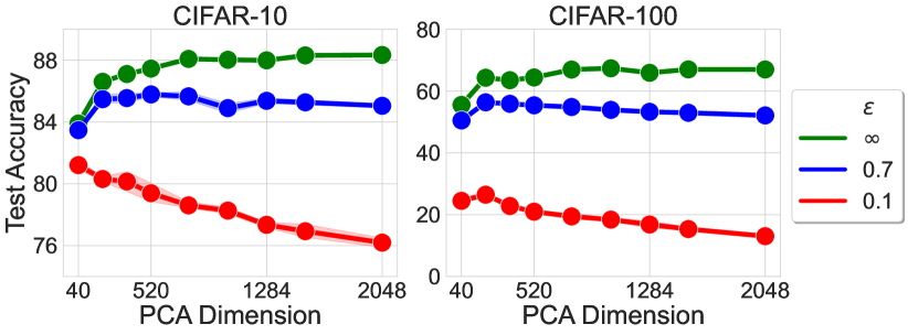
Figure 4: DP training of linear classifier on SL pre-trained feature using the PRV accountant. For non-DP training ($\epsilon=\infty$), accuracy increases as dimension increases; opposite occurs for DP training. For results on additional feature-extractors see Section B.6.

This observed dichotomy between private and non-private learning in terms of test accuracy and projection dimension aligns with Theorem 1 and Proposition 3 in Section 3.3. Theorem 1 indicates that that the private test accuracy improves as the projection dimension decreases, as depicted in Figure 4. For non-private training with moderately large dimension, ($k\geq 520$), the test accuracy remains largely constant. We discuss this theoretically in Proposition 3  Section 3.3. The decrease in non-private accuracy for very small values of $k$ is attributed to the increasing approximation error (i.e. how well can the best classifier in $k$ dimensions represent the ground truth). This difference in behaviour between private and non-private learning for decreasing $k$ values is observed consistently in all our experiments and is one of the main contributions of this paper. While we have demonstrated the effectiveness of our algorithm on the CIFAR-10 and CIFAR-100 benchmarks, as discussed in Section 5, we acknowledge that this evaluation setting may not fully reflect the actual objectives of private learning.

Pre-training		SL		BYOL
Private Algorithm	Additional Public Data	CIFAR10	CIFAR100	CIFAR10	CIFAR100
DP-SGD (Abadi et al., 2016)	None	84.89	50.65	79.85	46.12
JL (Nguyen et al., 2020)	None	84.40	50.56	78.92	43.13
AdaDPS (Li et al., 2022b)	Labelled	83.22	39.38	77.76	33.92
GEP (Yu et al., 2021)	Unlabelled	84.54	45.22	78.56	35.47
OURS	Unlabelled	85.89	55.86	80.89	46.94

Table 1: Comparison against baselines using publicly available code with comparable training settings. Here, using the RDP accountant for $\epsilon=0.7$. See Section B.5 for a discussion.

4.2 Comparison with Existing Methods

To ensure a fair comparison, we focus on the setting where $\epsilon=0.7$ and use the RDP accountant (Mironov, 2017) instead of the PRV accountant (Gopi et al., 2021a) employed throughout the rest of the paper. For a comprehensive discussion on the rationale behind this choice, implementation details, and the cross-validation ranges for hyper-parameters across all methods, refer to Section B.5

Baselines

We consider the following baselines:  i) DP-SGD(Abadi et al., 2016; Li et al., 2022c): Trains a linear classifier privately using DP-SGD on the pre-trained features. ii) JL(Nguyen et al., 2020): Applies a Johnson-Lindenstrauss (JL) transformation (without utilizing public data) to reduce the dimensionality of the features. We cross-validate various target dimensionalities and report the results for the most accurate one. iii) AdaDPS(Li et al., 2022b): Utilizes the public labeled data to compute the pre-conditioning matrix for adaptive optimization algorithms. Since our algorithm does not require access to labels for the public data, this comparison is deemed unfair. iv) GEP(Yu et al., 2021): Employs the public unlabeled data to decompose the private gradients into a low-dimensional embedding and a residual component, subsequently perturbing them with noise with different variance.

Whenever public data is utilized, we employ $10\%$ of the training data as public and remaining data as private. The official implementations of AdaDPS and GEP are used for our comparisons. In Section B.4, we discuss PATE (Papernot et al., 2017, 2018) and the reasons for not including it in our comparisons. For a detailed comparison with the work of De et al. (2022), including the use of a different feature extractor to ensure a fair evaluation, we refer to Section B.2, where we demonstrate that our method is competitive, if not superior, while being significantly computationally more efficient.

Results

In Table 1, we compare our approach with other methods in the literature. Our results suggest that reducing dimensionality by using the JL transformation is insufficient to even outperform DP-SGD. This may be attributed to the higher sample size required for their bounds to provide meaningful guarantees. Similarly, employing public data to pre-condition an adaptive optimizer does not result in improved performance for AdaDPS. Additionally, GEP also does not surpass DP-SGD, potentially due to its advantages being more pronounced in scenarios with much higher model dimensionality. Considering their lower performance on this simpler benchmark compared to DP-SGD and the extensive hyperparameter space that needs to be explored for most baselines, we focus on the strongest baseline (DP-SGD) for more challenging and realistic evaluation settings in Section 5.

5 Experimental Results Beyond Standard Benchmarks

In line with concurrent work (Tramèr et al., 2022), we raise concerns regarding the current trend of utilizing pre-trained feature extractors (De et al., 2022; Tramer and Boneh, 2021) for differentially private training. It is common practice to evaluate differentially private algorithms for image classification by pre-training on ImageNet-1K and performing private fine-tuning on CIFAR datasets (De et al., 2022; Tramer and Boneh, 2021). However, we argue that this approach may not yield generalisable insights for privacy-sensitive scenarios. Both ImageNet and CIFAR datasets primarily consist of everyday objects, and the label sets of ImageNet are partially included within CIFAR. Such a scenario is unrealistic for many privacy-sensitive applications, such as medical, finance, and satellite data, where a large publicly available pre-training dataset with similar characteristics to the private data may not be accessible.

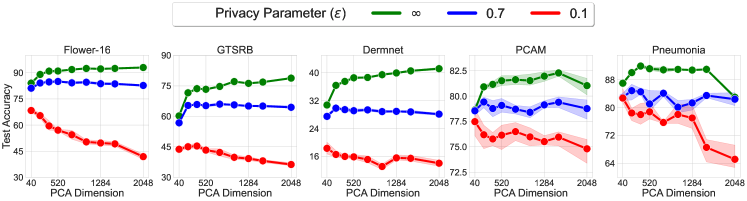
Figure 5: Test Accuracy of DP classification on Flower-16, GTSRB, Dermnet, PCAM, and Pneumonia for best pre-training algorithm (SL pre-training for Flower-16 and GTSRB and BYOL for the remaining.). For results on additional feature-extractors refer to Section B.6.

Moreover, public datasets are typically large-scale and easily scraped from the web, whereas private data is often collected on a smaller scale and subject to legal and competitive constraints, making it difficult to combine with other private datasets. Additionally, labeling private data, particularly in domains such as medical or biochemical datasets, can be costly. Therefore, evaluating the performance of privacy-preserving algorithms requires examining their robustness with respect to small dataset sizes. In order to address these considerations, we assess the performance of our algorithm on five additional datasets that exhibit varying degrees of distribution shift compared to the pre-training set, as described in Section 5.1. Furthermore, we also demonstrate the robustness of our algorithm to minor distribution shifts between public unlabeled and private labeled data. In Section 5.2, we show our algorithm is also robust to both small-sized private labeled datasets and public unlabeled datasets.

5.1 Effectiveness under Distribution Shift

Distribution Shift between Pre-Training and Private Data

We consider private datasets that exhibit varying levels of dissimilarity compared to the ImageNet pre-training dataset: Flower-16 (Flo, 2021), GTSRB (Houben et al., 2013), Pneumonia (Kermany et al., 2018), a fraction ($12.5\%$) of PCAM (Veeling et al., 2018), and DermNet (Der, 2019). In Figure 1, we provide visual samples from each of these datasets. Flower-16 and GTSRB have minimal overlap with ImageNet-1K, with only one class in Flower-16 and 43 traffic signs aggregated into a single label in ImageNet-1K. The Pneumonia, PCAM, and DermNet datasets do not share any classes with ImageNet-1K. We also observe that, given a fixed pre-training distribution and model, different training procedures can have a different impact in the utility of the extracted features for each downstream classification task. Therefore, for each dataset we report the best performance produced by the most useful pre-training algorithm. Results for all the 5 pre-training strategies we consider and a discussion of how to choose them is relegated to Section B.6.

	CIFAR10		CIFAR100
	SL	BYOL	SL	BYOL
In-distribution	81.21	72.33	27.47	19.89
CIFAR-10v1	81.18	73.24	27.18	19.21

(a) Distribution Shift between public (PCA) and private data

	CIFAR10		GTSRB
	SL	BYOL	SL	BYOL
1%	79.93	72.27	45.59	35.91
5%	81.02	72.33	45.64	35.88
10%	81.21	72.33	46.12	35.97

(b) Varying amounts of public (PCA) data

Table 2: a): Comparison between using the same amount of in-distribution data (i.e. 10% of CIFAR-10 and CIFAR-100 respectively) and CIFAR-10v1 for computing the PCA projection $(\epsilon=0.1)$. b) Performance of PILLARwith varying amounts of public (in distribution) data for computing the PCA projection ($\epsilon=0.1$). The amount of public data is presented as a fraction of the whole available dataset.

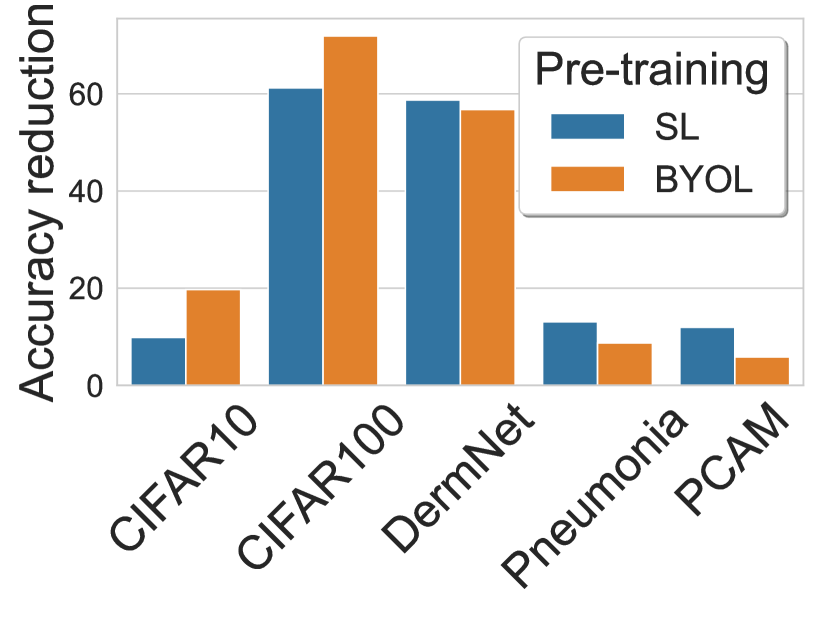
Figure 6: Comparing reduction in test accuracy for different datasets between using SL and BYOL pre-trained networks.

In Figure 5, we demonstrate that reducing the dimensionality of the pre-trained models enhances differentially private training, irrespective of the private dataset used. For instance, when applying the SL feature extractor to Flower-16 at at $\epsilon=0.1$ with $k=40$, the accuracy improves to $69.3\%$ compared to only $41.2\%$ when using the full dimensionality. For DermNet, PCAM, and Pneumonia at $\epsilon=0.1$, we observe accuracy improvements from $14\%$ to $19\%$, from $75\%$ to $77.5\%$, and from $65\%$ to $83\%$ respectively. Dimensionality reduction has a more pronounced effect on performance when tighter privacy constraints are imposed. It is worth noting that using dimensionality reduction can significantly degrade performance for non-DP training, as observed in CIFAR-10 and CIFAR-100.

When to use labels in pre-training

We also investigate the impact of different pre-training strategies on DP test accuracy. From Figure 4 and 5, we observe that some pre-trained models are more effective than others for specific datasets. To measure the maximum attainable accuracy with a publicly trained classifier, we compute the drop in performance, observed by training a DP classifier on BYOL pre-trained features, and the drop in performance for SL pre-trained features. We then plot the fractional reduction for both BYOL and SL across all the datasets for $\epsilon=0.1$ in Figure 6. In Figure 9 we compare the relative reduction in performance when using Semi-supervised pre-training and BYOL pre-training. We find that datasets with daily-life objects and semantic overlap with ImageNet-1K benefit more from leveraging SL features and thus have a smaller reduction in accuracy for SL features compared to BYOL features. In contrast, datasets with little label overlap with ImageNet-1K benefit more from BYOL features, consistent with findings by Shi et al. (2023).

Distribution Shift between $S^{U}$ and $S^{L}$

We demonstrate the effectiveness of our algorithm even when the public unlabeled data (used for computing the PCA projection matrix) is sourced from a slightly different distribution than the private labeled dataset. Specifically, we utilize the CIFAR-10v1 (Recht et al., 2018) dataset and present the results in Table 2(a). Notably, CIFAR-10v1 consists of only $2000$ samples ($4\%$ of the training data), yet the results for both CIFAR-10 and CIFAR-100 remain essentially unchanged. This finding indicates that the data used to compute the PCA projection matrix does not necessarily have to originate from the same distribution as the private data and underscores that large amounts of public data are not required for our method to be effective.

5.2 Effectiveness in Low-Data Regimes

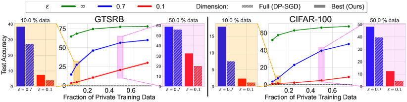
Figure 7: Middle columns: Test accuracy as the percentage of available training data varies in $\{0.05,0.1,0.25,0.5,0.75\}$. First and third columns: increase in test accuracy by applying PCA (solid bars) vs not reducing dimension (dashed bars) in low-data regimes for 50% (violet) and 10% (orange) private data.

In privacy-critical settings such as medical contexts, there is often a limited availability of training data. For instance, the DermNet and pneumonia datasets contain only 12,000 and 3,400 training data points, respectively, which is significantly smaller compared to datasets like CIFAR-10 with 50,000 samples. To examine the impact of reduced data (both private labeled and public unlabeled) on privacy, in this section we conduct ablations using different fractions of training data on the CIFAR-100 and GTSRB datasets. Please refer to Section B.1 for more details. .

Less private labelled data

In Figure 7, we present the performance of private and public training using different percentages of labeled training data for CIFAR-100 and GTSRB. Our results indicate that under stringent privacy constraints $\left({\epsilon\in\left\{{0,7,0.1}\right\}}\right)$, the performance of DP training, without dimensionality reduction, is considerably low. Conversely, even with a small percentage of training data, non-DP training demonstrates relatively high performance. By applying our algorithm in this scenario, we achieve significant performance improvements compared to using the full-dimensional embeddings. For instance, applying PCA with with $k=40$ dimensions enhances the accuracy of our proposed algorithm from $7.53\%$ to $18.3\%$ on $10\%$ of CIFAR-100, with $\epsilon=0.7$ using the SL feature extractor. Similar improvements are also shown for GTSRB and to a smaller extent for $\epsilon=0.1$

Less public unlabelled data

We demonstrate the robustness of our algorithm to reduced amounts of public unlabeled data. In Table 2(b), we vary the amount of public data and observe that the performance of our algorithm remains mostly stable despite decreasing amounts of public data.

6 Conclusion

In this paper, we consider the setting of semi-private learning where the learner has access to public unlabelled data in addition to private labelled data. This is a realistic setting in many circumstances e.g. where some people choose to make their data public. Under this setting, we proposed a new algorithm to learn linear halfspaces. Our algorithm uses a mix of PCA on unlabelled data and DP training on private data. Under reasonable theoretical assumptions, we have shown the proposed algorithm is $(\epsilon,\delta)$-DP and provably reduces the sample complexity. In practical applications, we performed an extensive set of experiments that show the proposed technique is effective when tight privacy constraints are imposed, even in low-data regimes and with a significant distribution shift between the pre-training and private distribution.

7 Acknowledgements

AS acknowledges partial support from the ETH AI Center Postdoctoral fellowship. FP acknowledges partial support from the European Space Agency. AS, FP, and YH also received funding from the Hasler Stiftung. We also thank Florian Tramer for useful feedback.

Appendix A Proofs

A.1 Noisy SGD

In this section, we present Algorithm 2, an adapted version of the Noisy SGD algorithm from Bassily et al. [2014b] for $d$-dimensional linear halfspaces $\mathcal{H}_{L}^{d}$, that is used as a sub-procedure in Algorithm 1. Algorithm 2 first applies a base procedure ${\mathcal{A}}_{Base}$ on $\mathcal{H}_{L}^{d}$ for $k$ times to generate a set of $k$ results while preserving $(\epsilon,\delta)$-DP, and then applies the exponential mechanism ${\mathcal{M}}_{E}$ to output one final result from the set.

Algorithm 2 ${\mathcal{A}}_{Noisy-SGD}(S^{L},\ell,(\epsilon,\delta),\beta)$

1:procedure ${\mathcal{A}}_{Noisy-SGD}$($S^{L},\ell,(\epsilon,\delta),\beta$)

2:     Input: a labelled dataset $S^{L}$, a loss function $\ell$, privacy parameters $\epsilon,\delta$, and the failure probability $\beta$.

3:     Set $k=\lceil\log\nicefrac{{1}}{{\beta}}\rceil$.

4:     for $i=1$ to $k$ do

5:         $\hat{w}^{(i)}\leftarrow{\mathcal{A}}_{Base}(S^{L},\ell,(\nicefrac{{\epsilon}}{{k}},\nicefrac{{\delta}}{{k}}))$

6:     end for

7:     Let ${\mathcal{O}}\leftarrow\{\hat{w}^{(1)},\ldots,\hat{w}^{(k)}\}$.

8:     $\hat{w}\leftarrow{\mathcal{M}}_{E}(S^{L},-\ell,{\mathcal{O}},\epsilon)$.

9:     Output: $\hat{w}$

10:end procedure

11:procedure ${\mathcal{A}}_{Base}$($(S^{L},\ell,(\epsilon,\delta))$)

12:     Input: a labelled dataset $S^{L}$, a loss function $\ell$, privacy parameters $\epsilon,\delta$.

13:     Let ${\mathcal{L}}$ be the Lipschitz coefficient of the loss function $\ell$ and $n^{L}$ be the size of $S^{L}$.

14:     Set noise variance $\sigma^{2}\leftarrow\frac{32L^{2}\left({n^{L}}\right)^{2}\log(n^{L}/\delta)\log(1/\delta)}{\epsilon}$.

15:     Randomize $\hat{w}^{0}\in\mathcal{H}_{L}^{d}$.

16:     Set the learning rate function $\eta(t)=\frac{1}{\sqrt{t(n^{L})^{2}{\mathcal{L}}^{2}+m\sigma^{2}}}$.

17:     for $t=1$ to $(n^{L})^{2}-1$ do

18:         Uniformly choose $(x,y)\in S^{L}$.

19:         Update $\hat{w}^{t+1}=\Pi_{{\mathcal{W}}}\left({\hat{w}_{t}-\eta(t)[n^{L}\nabla\ell(\hat{w}^{t};(x,y))+\xi]}\right)$ where $\xi\sim N(0,\mathbb{I}_{d}\sigma^{2})$.

20:     end for

21:     Output: $\hat{w}=\hat{w}^{(n^{L})^{2}}$

22:end procedure

23:procedure ${\mathcal{M}}_{E}$($S^{L},\ell,{\mathcal{O}},\epsilon$)

24:     Input: a dataset $S^{L}$, a loss function $\ell$, an set of parameters ${\mathcal{O}}$, and a privacy parameter $\epsilon$.

25:     Set the global sensitivity as $\Delta_{U}=\max_{S,S^{\prime}}\max_{w\in{\mathcal{O}}}|\ell(S,w)-\ell(S^{\prime},w)|$, for any $S,S^{\prime}$ of size $|S^{L}|$ differing at exactly one entry.

26:     Output: $w\in{\mathcal{O}}$ with probability proportional to $\exp\left({\frac{\epsilon\ell(S^{L},w)}{2\Delta_{U}}}\right)$.

27:end procedure

In Lemma 1, we state the privacy guarantee and the high probability upper bound on the excess error of the adpated version of Noisy SGD (Algorithm 2). This is a corollary of Theorem 2.4 in Bassily et al. [2014a], which provides an upper bound on the expected excess risk of ${\mathcal{A}}_{Base}$. The proof of Lemma 1 follows directly from Markov inequality and the post-processing property of DP (Lemma 2), as described in Appendix D of Bassily et al. [2014a].

Lemma 1 (Theoretical guarantees of Noisy SGD [Bassily et al., 2014b]).

Let the loss function $\ell$ be ${\mathcal{L}}$-Lipschitz and $\mathcal{H}_{L}^{d}$ be the $d$-dimensional linear halfspace with diameter $1$. Then ${\mathcal{A}}_{Noisy-SGD}$ is $(\epsilon,\delta)$-DP, and with probability $1-\beta$, its output $\hat{w}$ satisfies the following upper bound on the excess risk,

$$\sum_{(x,y)\in S}\ell(\hat{w},(x,y))-\sum_{(x,y)\in S}\ell(w^{\star},(x,y))=\frac{{\mathcal{L}}\sqrt{d}}{\epsilon}\cdot\text{polylog}(n,\frac{1}{\beta},\frac{1}{\delta}),$$

for a labelled dataset $S$ of size $n$. Here, $w^{\star}$ is the empirical risk minimizer $w^{\star}=\text{argmin}_{w\in{\mathcal{C}}}\sum_{(x,y)\in S}\ell(w,(x,y))$.

A.2 Proof of Theorem 1

See 1

Proof.

Privacy guarantee Algorithm ${\mathcal{A}}_{\epsilon,\delta}(k,\zeta)$ computes the transformation matrix $\hat{A}_{k}$ on the public unlabelled dataset. This step is independent of the labelled data $S^{L}$ and has no impact on the privacy with respect to $S^{L}$. ${\mathcal{A}}_{\mathrm{Noisy-SGD}}$ ensures the operations on the labelled dataset $S^{L}$ to output $v_{k}$ is $(\epsilon,\delta)$-DP with respect to $S^{L}$ (Lemma 1). The final output $\hat{w}=\hat{A}_{k}v_{k}$ is attained by post-processing of $v_{k}$ and preserves the privacy with respect to $S^{L}$ by the post-processing property of differential privacy (Lemma 2).

Lemma 2 (Post-processing [Dwork et al., 2006]).

For every $(\epsilon,\delta)$-DP algorithm ${\mathcal{A}}:S\rightarrow{\mathcal{Y}}$ and every (possibly random) function $f:{\mathcal{Y}}\rightarrow{\mathcal{Y}}^{\prime}$, $f\circ{\mathcal{A}}$ is $(\epsilon,\delta)$-DP.

Accuracy guarantee By definition, all distributions $D_{\gamma,\xi_{k}}\in{\mathcal{D}}_{\gamma_{0},\xi_{0}}$ are $(\gamma,\xi_{k})$-large margin low rank for some $\gamma\geq\gamma_{0},\xi_{k}\leq\xi_{0}$. Let the empirical covariance matrix of $D_{\gamma,\xi_{k}}$ calculated with the unlabelled dataset $S^{U}$ be $\widehat{\Sigma}=\frac{1}{n^{U}}\sum_{x\in S^{U}}(x-\bar{x})(x-\bar{x})^{\top}$ and $\hat{A}_{k}\in\mathbb{R}^{d\times k}$ be the projection matrix whose $i^{\it th}$ column is the $i^{\it th}$ eigenvector of $\widehat{\Sigma}$. Let $\Sigma$ be the population covariance matrix and similarly, let $A_{k}$ the matrix of top $k$ eigenvectors of $\Sigma$.

For any distribution $D_{\gamma,\xi_{k}}\in{\mathcal{D}}_{\gamma_{0},\xi_{0}}$, let $D_{X,\left({\gamma,\xi_{k}}\right)}$ be the marginal distribution of $X$ and $w^{\star}$ be the large margin linear classifier that is guaranteed to exist by Definition 3. The margin after projection by $\hat{A}_{k}$ is lower bounded by $\frac{y\left\langle{\hat{A}_{k}^{\top}z,\hat{A}_{k}^{\top}w^{\star}}\right\rangle}{\left\lVert\hat{A}_{k}^{T}z\right\rVert_{2}\left\lVert\hat{A}_{k}^{\top}w^{\star}\right\rVert_{2}}$ for any $z\in\mathop{\mathrm{supp}}\left({D_{X,\left({\gamma,\xi_{k}}\right)}}\right)$.

We will first derive a high-probability lower bound for this term to show that, after projection, with high probability, the projected distribution still has a large margin. Then, we will invoke existing algorithms in the literature with the right parameters, to privately learn a large margin classifier in this low-dimensional space.

Let $z$ be any vector in $\mathop{\mathrm{supp}}\left({D_{X,\left({\gamma,\xi_{k}}\right)}}\right)$. We can write $z=a_{z}w^{\star}+b^{\perp}$ for some $a_{z}$ where $b^{\perp}$ is in the nullspace of $w^{\star}$. Then, it is easy to see that using the large-margin property in Definition 3, we get

$$ya_{z}=\frac{\left\langle{w^{\star},z}\right\rangle}{\left\lVert w^{\star}\right\rVert_{2}\left\lVert z\right\rVert_{2}}\geq\gamma\geq\gamma_{0}.$$ (2)

Then, we lower bound $\dfrac{y\left\langle{\hat{A}_{k}^{\top}z,\hat{A}_{k}^{\top}w^{\star}}\right\rangle}{\left\lVert\hat{A}_{k}^{\top}z\right\rVert_{2}\left\lVert\hat{A}_{k}^{\top}w^{\star}\right\rVert_{2}}$ as

$$\frac{y\left\langle{\hat{A}_{k}^{\top}z,\hat{A}_{k}^{\top}w^{\star}}\right\rangle}{\left\lVert\hat{A}_{k}^{\top}z\right\rVert_{2}\left\lVert\hat{A}_{k}^{\top}w^{\star}\right\rVert_{2}} \overset{(a)}{=}\frac{ya_{z}\left\lVert\hat{A}_{k}^{\top}w^{\star}\right\rVert_{2}^{2}}{\left\lVert\hat{A}_{k}^{\top}z\right\rVert_{2}\left\lVert\hat{A}_{k}^{\top}w^{\star}\right\rVert_{2}}\overset{(b)}{\geq}\gamma_{0}\left\lVert\hat{A}_{k}^{\top}w^{\star}\right\rVert_{2}$$ (3)

where step $(a)$ is due to $\left\langle{w^{\star},b^{\perp}}\right\rangle=0$ and step $(b)$ follows from $\left\lVert\hat{A}_{k}^{\top}z\right\rVert_{2}\leq\left\lVert\hat{A}_{k}\right\rVert_{\text{op}}\left\lVert z\right\rVert_{2}\leq 1$ and Equation 2.

To lower bound $\left\lVert\hat{A}_{k}^{\top}w^{\star}\right\rVert_{2}$, note that

$$\left\lVert\hat{A}_{k}^{\top}w^{\star}\right\rVert_{2}=\left\lVert\hat{A}_{k}\hat{A}_{k}^{\top}w^{\star}\right\rVert_{2} \geq\left\lVert A_{k}A_{k}^{\top}w^{\star}\right\rVert_{2}-\left\lVert\hat{A}_{k}\hat{A}_{k}^{\top}w^{\star}-A_{k}A_{k}^{\top}w^{\star}\right\rVert_{2}$$ by Triangle Inequality (4)

$$\geq\left\lVert A_{k}A_{k}^{\top}w^{\star}\right\rVert_{2}-\left\lVert\hat{A}_{k}\hat{A}_{k}^{\top}-A_{k}A_{k}^{\top}\right\rVert_{F}\left\lVert w^{\star}\right\rVert_{2}$$ by Cauchy Schwarz Inequality

$$\geq 1-\xi_{k}-\left\lVert\hat{A}_{k}\hat{A}_{k}^{\top}-A_{k}A_{k}^{\top}\right\rVert_{F}.$$

where the last step follows from the low rank assumption in Definition 3 and observing that $\left\lVert w^{\star}\right\rVert_{2}=1$.

To upper bound $\left\lVert\hat{A}_{k}\hat{A}_{k}^{\top}-A_{k}A_{k}^{\top}\right\rVert_{F}$, we use Lemma 3.

Lemma 3 (Theorem 4 in Zwald and Blanchard [2005]).

Let $D$ be a distribution over $\{x\in\mathbb{R}^{d}|~{}\left\lVert x\right\rVert^{2}\leq 1\}$ with covariance matrix $\Sigma$ and zero mean ${\mathbb{E}}_{x\sim D}[x]=0$. For a sample $S$ of size $n$ from $D$, let $\widehat{\Sigma}=\frac{1}{n}\sum_{x\in S}xx^{T}$ be the empirical covariance matrix. Let $A_{k},\hat{A}_{k}$ be the matrices whose columns are the first $k$ eigenvectors of $\Sigma$ and $\widehat{\Sigma}$ respectively and let $\lambda_{1}\left({\Sigma}\right)>\lambda_{2}\left({\Sigma}\right)>\ldots>\lambda_{d}\left({\Sigma}\right)$ be the ordered eigenvalues of $\Sigma$. For any $k>0,\beta\in\left({0,1}\right)$ such that $\lambda_{k}\left({\Sigma}\right)>0$ and $n\geq\frac{16\left({1+\sqrt{\beta/2}}\right)^{2}}{\left({\lambda_{k}\left({\Sigma}\right)-\lambda_{k+1}\left({\Sigma}\right)}\right)^{2}}$, we have that with probability at least $1-e^{-\beta}$,

$$\left\lVert A_{k}A_{k}^{T}-\hat{A}_{k}\hat{A}_{k}^{T}\right\rVert_{F}\leq\frac{4\left({1+\sqrt{\frac{\beta}{2}}}\right)}{\left({\lambda_{k}\left({\Sigma}\right)-\lambda_{k+1}\left({\Sigma}\right)}\right)\sqrt{n}}.$$

It guarantees that with probability $1-\frac{\beta}{2}$,

$$\left\lVert A_{k}A_{k}^{\top}-\hat{A}_{k}\hat{A}_{k}^{\top}\right\rVert_{F}\leq\frac{4\left({1+\sqrt{\frac{\log\left({\nicefrac{{2}}{{\beta}}}\right)}{2}}}\right)}{\left({\lambda_{k}\left({\Sigma}\right)-\lambda_{k+1}\left({\Sigma}\right)}\right)\sqrt{n^{U}}}\leq\frac{\gamma_{0}}{10}.$$ (5)

where the last inequality follows from choosing the size of unlabelled data $n^{U}\geq\frac{1600\left({1+\sqrt{\frac{\log\left({\nicefrac{{2}}{{\beta}}}\right)}{2}}}\right)^{2}}{\gamma_{0}^{2}\left({\Delta_{\min}\lambda_{k}}\right)^{2}}$.

Substituting Equation 5 into Equation 4, we get that with probability $1-\frac{\beta}{2}$,

$$\left\lVert\hat{A}_{k}^{\top}w^{\star}\right\rVert_{2}\geq 1-\xi_{k}-\frac{\gamma}{10}$$ (6)

Plugging Equation 6 into Equation 3, we derive a high-probability lower bound on the distance of any point to the decision boundary in the transformed space. For all $z\in\mathop{\mathrm{supp}}\left({D_{X,\left({\gamma,\xi_{k}}\right)}}\right)$,

$$\frac{y\left\langle{\hat{A}_{k}^{\top}z,\hat{A}_{k}^{\top}w^{\star}}\right\rangle}{\left\lVert\hat{A}_{k}^{\top}z\right\rVert_{2}\left\lVert\hat{A}_{k}^{\top}w^{\star}\right\rVert_{2}}\geq\gamma_{0}\left({1-\xi_{0}-\frac{\gamma_{0}}{10}}\right).$$

This implies that the margin in the transformed space is at least $\gamma_{0}\left({1-\xi_{0}-\nicefrac{{\gamma_{0}}}{{10}}}\right)$. Thus, the (scaled) hinge loss function $\ell$ defined in Equation 1 is $\frac{1}{\gamma_{0}\left({1-\xi_{0}-\nicefrac{{\gamma_{0}}}{{10}}}\right)}$-Lipschitz. For a halfspace with parameter $v\in B_{2}^{k}$, denote the empirical hinge loss on a dataset $S$ by $\hat{L}(w;S)=\frac{1}{\left|{S}\right|}\sum_{(x,y)\in S}\ell(w,(x,y))$ and the loss on the distribution $D$ by $L(w;D)={\mathbb{P}}_{(x,y)\sim D}\left[{\ell(w,(x,y))}\right]$. Let $D_{k}$ be the $k$-dimension transformation of the original distribution $D$ obtained by projecting each $x\in{\mathcal{X}}$ to $\hat{A}_{k}^{\top}x$. By the convergence bound in Lemma 1 for ${\mathcal{A}}_{\mathrm{Noisy-SGD}}$, we have with probability $1-\frac{\beta}{4}$, ${\mathcal{A}}_{\mathrm{Noisy-SGD}}$ outputs a hypothesis $v_{k}\in B_{2}^{k}$ such that

$$\hat{L}(v_{k};S^{L}_{k})-\hat{L}(v_{k}^{\star};D_{k})=\hat{L}(v_{k};S^{L}_{k})=\tilde{O}\left({\frac{\sqrt{k}}{n^{L}\epsilon\gamma_{0}\left({1-\xi_{0}-0.1\gamma_{0}}\right)}}\right)$$

where $v_{k}^{\star}=\text{argmin}_{v\in B_{2}^{k}}\hat{L}(v;S^{L}_{k})$ and $\hat{L}(v_{k}^{\star};S^{L}_{k})=0$ as the margin in the transformed space is at least $\gamma_{0}\left({1-\xi_{0}-\frac{\gamma_{0}}{10}}\right)\geq 0$.

Then, we can upper bound the empirical 0-1 error by the empirical (scaled) hinge loss in the $k$-dimensional transformed space. For $n^{L}=\left({\frac{\sqrt{k}}{\alpha\epsilon\gamma_{0}(1-\xi_{0}-0.1\gamma_{0})}}\right)\mathrm{polylog}\left(\frac{1}{\delta},\frac{1}{\epsilon},\frac{1}{\beta},\frac{1}{\alpha},\frac{1}{\gamma_{0}},\frac{1}{\xi_{0}},k,n^{L}\right)$, with probability $1-\frac{\beta}{4}$,

$$\frac{1}{n^{L}}\sum_{(x,y)\in S^{L}}\mathbbm{I}\{y\left\langle{x,v_{k}}\right\rangle<0\}\leq\hat{L}(v_{k};S^{L}_{k})=\tilde{O}\left({\frac{\sqrt{k}}{n^{L}\epsilon\gamma_{0}\left({1-\xi_{0}-0.1\gamma_{0}}\right)}}\right)\leq\frac{\alpha}{4}$$ (7)

It remains to bound the generalisation error of linear halfspaces $\mathcal{H}_{L}^{k}$. That is, we still need to show that the empirical error of a linear halfspace is a good approximation of the error on the distribution. To achieve this, we can apply Lemma 4 to upper bound the generalisation error using the growth function.

Lemma 4 (Convergence bound on generalisation error [Anthony and Bartlett, 1999]).

Suppose ${\mathcal{H}}$ is a hypothesis class with instance space ${\mathcal{X}}$ and output space $\{-1,1\}$. Let $D$ be a distribution over ${\mathcal{X}}\times{\mathcal{Y}}$ and $S$ be a dataset of size $n$ sampled i.i.d. from $D$. For $\eta\in(0,1),\zeta>0$, we have

$${\mathbb{P}}_{S\sim D^{n}}\left[{\sup_{h\in{\mathcal{H}}}L(h;D)-(1+\zeta)\hat{L}(h;S)>\eta}\right]\leq 4\Pi_{{\mathcal{H}}}(2n)\exp\left({-\frac{\eta\zeta n}{4\left({\zeta+1}\right)}}\right),$$

where $L$ and $\hat{L}$ are the population and the empirical 0-1 error and $\Pi_{{\mathcal{H}}}$ is the growth function of ${\mathcal{H}}$.

As the Vapnik-Chervonenkis (VC) dimension of $k$-dimensional linear halfspaces is $k+1$, its growth function is bounded by $\Pi(2n^{L})\leq(2n^{L})^{k+1}+1$. Setting $\eta=\frac{\alpha}{2},\zeta=1$ in Lemma 4 and combining with Equation 7, we have that with probability $1-\frac{\beta}{4}$, we have

$${\mathbb{P}}_{(x,y)\sim D}\left[{y\left\langle{v_{k},\hat{A}_{k}^{\top}x}\right\rangle<0}\right]={\mathbb{P}}_{(x,y)\sim D_{k}}\left[{y\left\langle{v_{k},x}\right\rangle<0}\right]\leq\frac{2}{n^{L}}\sum_{(x,y)\in S^{L}_{k}}\mathbbm{I}\{y\left\langle{v_{k},x}\right\rangle\leq 0\}+\frac{\alpha}{2}\leq\alpha,$$

for $n^{L}\geq\frac{k}{\alpha}\mathrm{polylog}\left({\frac{1}{\beta},\frac{1}{k}}\right)$. This is equivalent as stating that the output of Algorithm 1 $\hat{w}=\hat{A}_{k}v_{k}$ satisfies

$${\mathbb{P}}_{(x,y)\sim D}\left[{y\left\langle{\hat{w},x}\right\rangle<0}\right]\overset{(a)}{=}{\mathbb{P}}_{(x,y)\sim D}\left[{y\left\langle{\hat{A}_{k}v_{k},x}\right\rangle<0}\right]\overset{(b)}{=}{\mathbb{P}}_{(x,y)\sim D}\left[{y\left\langle{v_{k},\hat{A}_{k}^{\top}x}\right\rangle<0}\right]\leq\alpha,$$

where Equality $(a)$ follows from the definition of $\hat{w}=\hat{A}_{k}v_{k}$ and Equality $(b)$ follows from the definition of $k$-dimensional transformation $D_{k}$ of a distribution $D$. This concludes the proof. ∎

A.3 Privacy guarantees for PILLAR on the original image dataset

As described in Figure 2, in practice PILLAR is applied on the set of representations obtained by passing the private dataset of images through a pre-trained feature extractor. Therefore, a straightforward application of Theorem 1 yields an $\left({\epsilon,\delta}\right)$-DP guarantee on the set of representations and not on the dataset in the raw pixel space themselves. Here, we show that PILLAR provides (at least) the same DP guarantees on the dataset in the pixel space as long as the pre-training dataset cannot be manipulated by the privacy adversary. One way to achieve this, as we show is possible in this paper, is by using the same pre-trained model across different tasks. Investigating the extent of privacy harm that can be caused by allowing the adversary to manipulate the pre-training data remains an important future direction.

Corollary 4.

Let $f:\mathbb{R}^{p}\to\mathbb{R}^{d}$ be a feature extractor pre-trained using any algorithm. Let $S_{1},S_{2}$ be any two neighbouring datasets of private images in $\mathbb{R}^{p}$. Then, for any $Q\subseteq\mathcal{H}_{L}^{d}$ where $\mathcal{H}_{L}^{d}$ is the class of linear halfspaces in $d$ dimensions,

$${\mathbb{P}}_{h\sim{\mathcal{A}}_{\epsilon,\delta}\circ f\left({S_{1}}\right)}\left[{h\in Q}\right]\leq e^{\epsilon}{\mathbb{P}}_{h\sim{\mathcal{A}}_{\epsilon,\delta}\circ f\left({S_{2}}\right)}\left[{h\in Q}\right]+\delta$$

where ${\mathcal{A}}_{\epsilon,\delta}$ is Algorithm 1 (PILLAR) run with privacy parameters $\epsilon,\delta$.

Proof.

Note that $f$ is a deterministic many-to-one function from the dataset of images to the dataset of representations . For any two neighbouring datasets $S_{1},S_{2}$ in the image space, let $S^{\text{R}}_{1},S^{\text{R}}_{2}$ be the corresponding set of representations extracted by $f$, i.e. $S^{\text{R}}_{1}=\left\{{f(x):x\in S_{1}}\right\}$ and $S^{\text{R}}_{2}=\left\{{f(x):x\in S_{2}}\right\}$. Then for any $Q\subseteq\mathcal{H}_{L}^{d}$

$${\mathbb{P}}_{h\sim{\mathcal{A}}_{\epsilon,\delta}\circ f\left({S_{1}}\right)}\left[{h\in Q}\right] ={\mathbb{P}}_{h\sim{\mathcal{A}}_{\epsilon,\delta}\left({S^{\text{R}}_{1}}\right)}\left[{h\in Q}\right]$$

$$\leq e^{\epsilon}{\mathbb{P}}_{h\sim{\mathcal{A}}_{\epsilon,\delta}\left({S^{\text{R}}_{2}}\right)}[h\in Q]+\delta$$

$$=e^{\epsilon}{\mathbb{P}}_{h\sim{\mathcal{A}}_{\epsilon,\delta}\circ f\left({S_{2}}\right)}\left[{h\in Q}\right]+\delta$$

where the first and the last equality follows by using the definition $S^{\text{R}}_{1},S^{\text{R}}_{2}$ and due to the fact that $f$ is a many-to-one function. The second inequality follows from observing that $S^{\text{R}}_{1},S^{\text{R}}_{2}$ can differ on at most one point as $f$ is a deterministic many-to-one function and ${\mathcal{A}}_{\epsilon,\delta}$ is $\left({\epsilon,\delta}\right)$-DP. ∎

A.4 Proof of Theorem 2

In this section, we restate Theorem 2 with additional details and present its proof. Before that, we formally define $\eta$-TV tolerant semi-private learning.

Definition 4 ($\eta$-TV tolerant $(\alpha,\beta,\epsilon,\delta)$-semi-private learner on a family of distributions ${\mathcal{D}}$).

An algorithm ${\mathcal{A}}$ is an $\eta$-TV tolerant $(\alpha,\beta,\epsilon,\delta)$-semi-private learner for a hypothesis class ${\mathcal{H}}$ on a family of distributions ${\mathcal{D}}$ if for any distribution $D^{L}\in{\mathcal{D}}$, given a labelled dataset $S^{L}$ of size $n^{L}$ sampled i.i.d. from $D^{L}$ and an unlabelled dataset $S^{U}$ of size $n^{U}$ sampled i.i.d. from any distribution $D^{U}$ with $\eta$-bounded TV distance from $D^{L}_{X}$ as well as third moment bounded by $\eta$, ${\mathcal{A}}$ is $(\epsilon,\delta)$-DP with respect to $S^{L}$ and outputs a hypothesis $h$ satisfying

$${\mathbb{P}}[{\mathbb{P}}_{(x,y)\sim D}\left[{h(x)\neq y}\right]\leq\alpha]\geq 1-\beta,$$

where the outer probability is over the randomness of the samples and the intrinsic randomness of the algorithm. In addition, the sample complexity $n^{L}$ and $n^{U}$ must be polynomial in $\frac{1}{\alpha}$ and $\frac{1}{\beta}$, and $n^{L}$ must also be polynomial in $\frac{1}{\epsilon}$ and $\frac{1}{\delta}$.

Now, we are ready to prove that PILLAR is an $\eta$-TV tolerant $(\alpha,\beta,\epsilon,\delta)$-semi-private learner when instantiated with the right arguments.

Theorem 5.

For $k\leq d\in{\mathbb{N}},~{}\gamma_{0}\in(0,1),~{}\xi_{0}\in[0,1)$ satisfying $\xi_{0}<\nicefrac{{1}}{{2}}-\nicefrac{{\gamma_{0}}}{{10}}$, let ${\mathcal{D}}_{\gamma_{0},\xi_{0}}$ be the family of distributions consisting of all $\left({\gamma,\xi_{k}}\right)$-large margin low rank distributions over ${\mathcal{X}}_{d}\times{\mathcal{Y}}$ with $\gamma\geq\gamma_{0}$ and $\xi_{k}\leq\xi_{0}$ and third moment bounded by $\eta$. For any $\alpha\in\left({0,1}\right),\beta\in\left({0,\nicefrac{{1}}{{4}}}\right)$, $\epsilon\in\left({0,\nicefrac{{1}}{{\sqrt{k}}}}\right)$, $\delta\in(0,1)$ and $\eta\in[0,\nicefrac{{\Delta_{k}}}{{14}})$, ${\mathcal{A}}_{\epsilon,\delta}(k,\zeta)$, described by Algorithm 1, is an $\eta$-TV tolerant $(\alpha,\beta,\epsilon,\delta)$-semi-private learner of the linear halfspace $\mathcal{H}_{L}^{d}$ on ${\mathcal{D}}_{\gamma_{0},\xi_{0}}$ with sample complexity

$$n^{U}=O\left(\frac{\log\frac{2}{\beta}}{\left({\gamma_{0}\Delta_{k}}\right)^{2}}\right),n^{L}=\tilde{O}\left({\frac{\sqrt{k}}{\alpha\epsilon\zeta}}\right)$$

where $\Delta_{k}=\lambda_{k}\left({\Sigma^{L}}\right)-\lambda_{k+1}\left({\Sigma^{L}}\right)$ and $\zeta=\gamma_{0}(1-\xi_{0}-0.1\gamma_{0}-\nicefrac{{7\eta}}{{\Delta_{k}}})$.

Proof.

Privacy Guarantee A similar argument as the proof of the privacy guarantee in Theorem 1 shows that Algorithm ${\mathcal{A}}_{\epsilon,\delta}(k,\zeta)$ preserves $(\epsilon,\delta)$-DP on the labelled dataset $S^{L}$. We now focus on the accuracy guarantee.

Accuracy Guarantee For any unlabelled distribution $D^{U}$ with $\eta$-bouneded TV distance from the labelled distribution $D_{\gamma,\xi_{k}}^{L}$, let the empirical covariance matrix of the unlabelled dataset $S^{U}$ be $\widehat{\Sigma}^{U}=\frac{1}{n^{U}}\sum_{x\in S^{U}}xx^{\top}$ and $\hat{A}_{k}\in\mathbb{R}^{d\times k}$ be the projection matrix whose $i^{\it th}$ column is the $i^{\it th}$ eigenvector of $\widehat{\Sigma}^{U}$. Let $\Sigma^{L}$ and $\Sigma^{U}$ be the population covariance matrices of the labelled and unlabelled distributions $D^{L}$ and $D^{U}$. Similarly, let $A_{k}^{L}$ and $A_{k}^{U}$ be the matrices of top $k$ eigenvectors of $\Sigma^{L}$ and $\Sigma^{U}$ respectively.

By definition, all distributions $D_{\gamma,\xi_{k}}^{L}\in{\mathcal{D}}_{\gamma_{0},\xi_{0}}$ are $(\gamma,\xi_{k})$-large margin low rank distribution, as defined in Definition 3, for some $\gamma\geq\gamma_{0}$, $\xi_{k}\leq\xi_{0}$. Let $w^{\star}$ be the large margin linear classifier that is guaranteed to exist by Definition 3. Then, for all $z\in\mathop{\mathrm{supp}}\left({D_{X,(\gamma,\xi_{0})}^{L}}\right)$, where $D_{X,(\gamma,\xi_{0})}^{L}$ is the marginal distribution of $D_{\gamma,\xi_{k}}$, its margin is lower bounded by $\frac{y\left\langle{\hat{A}_{k}^{\top}z,\hat{A}_{k}^{\top}w^{\star}}\right\rangle}{\left\lVert\hat{A}_{k}^{\top}z\right\rVert_{2}\left\lVert\hat{A}_{k}^{\top}w^{\star}\right\rVert_{2}}$. Similar to the proof of Theorem 1, we will first lower bound this term to show that, with high probability, the projected distribution still retains a large margin. Then, we will invoke existing algorithms in the literature with the right parameters, to privately learn a large margin classifier in this low dimensional space.

First, let $z=a_{z}w^{\star}+b^{\perp}$ for some $a_{z}$ where $b^{\perp}$ is in the nullspace of $w^{\star}$. Then, it is easy to see that using the large-margin property in Definition 3, we get

$$ya_{z}=\frac{\left\langle{w^{\star},z}\right\rangle}{\left\lVert w^{\star}\right\rVert_{2}\left\lVert z\right\rVert_{2}}\geq\gamma\geq\gamma_{0}.$$ (8)

Then, we lower bound $\dfrac{y\left\langle{\hat{A}_{k}^{\top}z,\hat{A}_{k}^{\top}w^{\star}}\right\rangle}{\left\lVert\hat{A}_{k}^{\top}z\right\rVert_{2}\left\lVert\hat{A}_{k}^{\top}w^{\star}\right\rVert_{2}}$ as

$$\frac{y\left\langle{\hat{A}_{k}^{\top}z,\hat{A}_{k}^{\top}w^{\star}}\right\rangle}{\left\lVert\hat{A}_{k}^{\top}z\right\rVert_{2}\left\lVert\hat{A}_{k}^{\top}w^{\star}\right\rVert_{2}} \overset{(a)}{=}\frac{ya_{z}\left\lVert\hat{A}_{k}^{\top}w^{\star}\right\rVert_{2}}{\left\lVert\hat{A}_{k}^{\top}z\right\rVert_{2}}\overset{(b)}{\geq}\gamma_{0}\left\lVert\hat{A}_{k}^{\top}w^{\star}\right\rVert_{2},$$ (9)

where step $(a)$ is due to $\left\langle{w^{\star},b^{\perp}}\right\rangle=0$ and step $(b)$ follows from $\left\lVert\hat{A}_{k}^{\top}z\right\rVert_{2}\leq\left\lVert\hat{A}_{k}\right\rVert_{\text{op}}\left\lVert z\right\rVert_{2}\leq 1$ and Equation 8. To lower bound $\left\lVert\hat{A}_{k}^{\top}w^{\star}\right\rVert_{2}$, we use the triangle inequality to decompose it as follows

$$\left\lVert\hat{A}_{k}^{\top}w^{\star}\right\rVert_{2}\geq \left\lVert A_{k}^{L}\left({A_{k}^{L}}\right)^{\top}w^{\star}\right\rVert_{2}-\left\lVert\left({A_{k}^{L}\left({A_{k}^{L}}\right)^{\top}-A_{k}^{U}\left({A_{k}^{U}}\right)^{\top}}\right)w^{\star}\right\rVert_{2}-\left\lVert\left({A_{k}^{U}(A_{k}^{U})^{\top}-\hat{A}_{k}(\hat{A}_{k})^{\top}}\right)w^{\star}\right\rVert_{2}$$ (10)

$$\geq \left\lVert A_{k}^{L}\left({A_{k}^{L}}\right)^{\top}w^{\star}\right\rVert_{2}-\left\lVert A_{k}^{L}(A_{k}^{L})^{\top}-A_{k}^{U}\left({A_{k}^{U}}\right)^{\top}\right\rVert_{\text{op}}\left\lVert w^{\star}\right\rVert_{2}-\left\lVert A_{k}^{U}(A_{k}^{U})^{\top}-\hat{A}_{k}(\hat{A}_{k})^{\top}\right\rVert_{F}\left\lVert w^{\star}\right\rVert_{2}$$

$$\geq 1-\xi_{k}-\left\lVert A_{k}^{L}(A_{k}^{L})^{\top}-A_{k}^{U}\left({A_{k}^{U}}\right)^{\top}\right\rVert_{\text{op}}-\left\lVert A_{k}^{U}(A_{k}^{U})^{\top}-\hat{A}_{k}(\hat{A}_{k})^{\top}\right\rVert_{F}$$

where the second inequality follows from applying Cauchy-Schwartz inequality on the second and third term and the third step follows from using the low rank separability assumption in Definition 3 on the first term and observing that $\left\lVert w^{\star}\right\rVert_{2}=1$.

Now, we need to bound the two terms $\left\lVert A_{k}^{L}(A_{k}^{L})^{\top}-A_{k}^{U}\left({A_{k}^{U}}\right)^{\top}\right\rVert_{\text{op}}$,$\left\lVert A_{k}^{U}(A_{k}^{U})^{\top}-\hat{A}_{k}(\hat{A}_{k})^{\top}\right\rVert_{F}$. We bound the first term with Lemma 5.

Lemma 5 (Theorem 3 in Zwald and Blanchard [2005]).

Let $A\in{\mathbb{R}}^{d}$ be a symmetric positive definite matrix with nonzero eigenvalues $\lambda_{1}>\lambda_{2}>\ldots>\lambda_{d}$. Let $k>0$ be an integer such that $\lambda_{k}>0$. Let $B\in{\mathbb{R}}^{d}$ be another symmetric positive definite matrix such that $\left\lVert B\right\rVert_{F}<\frac{1}{4}\left({\lambda_{k}-\lambda_{k+1}}\right)$ and $A+B$ is still a positive definite matrix. Let $P_{k}(A),P_{k}(A+B)$ be the matrices whose columns consists of the first $k$ eigenvectors of $A,A+B$, then

$$\left\lVert P_{k}(A)P_{k}(A)^{T}-P_{k}(A+B)P_{k}(A+B)^{T}\right\rVert_{F}\leq\frac{2\left\lVert B\right\rVert_{F}}{\lambda_{k}-\lambda_{k+1}}.$$

It guarantees that with probability $1-\nicefrac{{\beta}}{{4}}$,

$$\left\lVert A_{k}^{L}\left({A_{k}^{L}}\right)^{\top}-A_{k}^{U}\left({A_{k}^{U}}\right)^{\top}\right\rVert_{\text{op}}\leq\frac{2\left\lVert\Sigma^{L}-\Sigma^{U}\right\rVert_{\text{op}}}{\lambda_{k}\left({\Sigma^{L}}\right)-\lambda_{k+1}\left({\Sigma^{L}}\right)}$$ (11)

Then, we bound the term $\left\lVert\Sigma^{L}-\Sigma^{U}\right\rVert_{\text{op}}$ with Lemma 6.

Lemma 6.

Let $f$ and $g$ be the Probability Density Functions (PDFs) of two zero-mean distributions $F$ and $G$ over ${\mathcal{X}}$ with covariance matrices $\Sigma_{f}$ and $\Sigma_{g}$ respectively. Assume the spectral norm of the third moments of both $F$ and $G$ are bounded by $\eta$. If the total variation between the two distributions is bounded by $\eta$,i.e. $TV(f,g)=\max_{A\subset{\mathcal{X}}}\left|{f(A)-g(A)}\right|\leq\eta$, then the discrepancy in the covariance matrices is bounded by $7\eta$, i.e.$\left\lVert\Sigma_{f}-\Sigma_{g}\right\rVert_{\text{op}}\leq 7\eta$.

By applying Lemma 6 and the assumption of bounded total variation between the labelled and unlabelled distributions to Equation 11, we get

$$\left\lVert A_{k}^{L}\left({A_{k}^{L}}\right)^{\top}-A_{k}^{U}\left({A_{k}^{U}}\right)^{\top}\right\rVert_{\text{op}}\leq\frac{7\eta}{\lambda_{k}\left({\Sigma^{L}}\right)-\lambda_{k+1}\left({\Sigma^{L}}\right)}=\frac{7\eta}{\Delta_{k}},$$ (12)

Similar to the proof for Theorem 1, we upper bound the term $\left\lVert A_{k}^{U}(A_{k}^{U})^{\top}-\hat{A}_{k}(\hat{A}_{k})^{\top}\right\rVert_{F}$ using Lemma 3, which guarantees that with probability $1-\nicefrac{{\beta}}{{4}}$,

$$\left\lVert A_{k}^{U}\left({A_{k}^{U}}\right)^{\top}-\hat{A}_{k}\hat{A}_{k}^{\top}\right\rVert_{F}\leq\frac{\gamma_{0}}{10},$$ (13)

where the inequality follows from choosing the size of unlabelled data $n^{U}=O\left(\frac{\log\frac{2}{\beta}}{\left({\gamma_{0}\Delta_{k}}\right)^{2}}\right)$.

Substituting Equations 13 and 12 into Equation 10 and then plugging Equation 10 into Equation 9, we get that with probability at least $1-\nicefrac{{\beta}}{{2}}$, the margin in the projected space is lower bounded as

$$\frac{y\left\langle{\hat{A}_{k}^{\top}z,\hat{A}_{k}^{\top}w^{\star}}\right\rangle}{\left\lVert\hat{A}_{k}^{\top}z\right\rVert_{2}\left\lVert\hat{A}_{k}^{\top}w^{\star}\right\rVert_{2}}\geq\gamma_{0}\left({1-\xi_{0}-\frac{7\eta}{\Delta_{k}}-\frac{\gamma_{0}}{10}}\right).$$

Thus, the (scaled) hinge loss function $\ell$ defined in Equation 1 in Algorithm 1 is $\frac{1}{\gamma_{0}\left({1-\xi_{0}-\nicefrac{{7\eta}}{{\Delta_{k}}}-0.1\gamma_{0}}\right)}$-Lipschitz. For a halfspace with parameter $v\in B_{2}^{k}$, denote the empirical hinge loss on a dataset $S$ by $\hat{L}(w;S)=\frac{1}{|S|}\sum_{(x,y)\in S}\ell(w,(x,y))$ and the loss on the distribution $D$ by $L(w;D)={\mathbb{E}}_{(x,y)\sim D}\left[{\ell(w,(x,y))}\right]$. Let $D_{k}$ be the $k$-dimension transformation of the original distribution $D$ by projecting each $x\in{\mathcal{X}}$ to $\hat{A}_{k}^{\top}x$. By the convergence bound in Lemma 1 for ${\mathcal{A}}_{\mathrm{Noisy-SGD}}$, we have with probability $1-\frac{\beta}{4}$, ${\mathcal{A}}_{\mathrm{Noisy-SGD}}$ outputs a hypothesis $v_{k}\in B_{2}^{k}$ such that

$$\hat{L}(v_{k};S^{L}_{k})-\hat{L}(v_{k}^{\star};D_{k})=\hat{L}(v_{k};S^{L}_{k})=\tilde{O}\left({\frac{\sqrt{k}}{n^{L}\epsilon\gamma_{0}\left({1-\xi_{0}-\nicefrac{{7\eta}}{{\Delta_{k}}}-0.1\gamma_{0}}\right)}}\right),$$

where $v_{k}^{\star}=\text{argmin}_{v\in B_{2}^{k}}\hat{L}(v;S^{L}_{k})$ and $\hat{L}(v_{k}^{\star};S^{L}_{k})=0$ as the margin in the transformed low-dimensional space is at least $\gamma_{0}(1-\xi_{0}-\frac{7\eta}{\Delta_{k}}-\frac{\gamma_{0}}{10}>0$. For $n^{L}=O\left({\frac{\sqrt{k}}{\alpha\beta\gamma_{0}\left({1-\xi_{0}-\nicefrac{{7\eta}}{{\Delta_{k}}}-0.1\gamma_{0}}\right)}\text{polylog}\left({\frac{1}{\delta},\frac{1}{\epsilon},\frac{1}{\beta},\frac{1}{\alpha},\frac{1}{\gamma_{0}},\frac{1}{\xi_{0}},k,n^{L}}\right)}\right)$, we can bound the emiprical 0-1 error with probability $1-\frac{\beta}{4}$,

$$\frac{1}{n^{L}}\sum_{(x,y)\in S^{L}_{k}}\mathbbm{I}\left\{{y\left\langle{v_{k},x}\right\rangle<0}\right\}\leq\hat{L}(v_{k};S^{L}_{k})=\tilde{O}\left({\frac{\sqrt{k}}{n^{L}\epsilon\gamma_{0}\left({1-\xi_{0}-\nicefrac{{7\eta}}{{\Delta_{k}}}-0.1\gamma_{0}}\right)}}\right)\leq\frac{\alpha}{4}.$$ (14)

It remains to bound the generalisation error of linear halfspace $\mathcal{H}_{L}^{k}$. Similar to the proof of Theorem 1, setting $\zeta=1$ and $\eta=\frac{\alpha}{2}$ and invoking Lemma 4 gives us that with probability $1-\frac{\beta}{4}$,

$${\mathbb{P}}_{(x,y)\sim D_{k}}\left[{y\left\langle{v_{k},x}\right\rangle<0}\right]-\frac{2}{n^{L}}\sum_{(x,y)\in S^{L}_{k}}\mathbbm{I}\{y\left\langle{v_{k},x}\right\rangle<0\}\leq\frac{\alpha}{2}.$$ (15)

Thus, combining Equations 14 and 15 we get

$${\mathbb{P}}_{(x,y)\sim D}\left[{y\left\langle{v_{k},\hat{A}_{k}^{\top}x}\right\rangle<0}\right]={\mathbb{P}}_{(x,y)\sim D_{k}}\left[{y\left\langle{v_{k},x}\right\rangle<0}\right]\leq\frac{2}{n^{L}}\sum_{(x,y)\in S^{L}_{k}}\mathbbm{I}\{y\left\langle{v_{k},x}\right\rangle<0\}+\frac{\alpha}{2}=\alpha,$$

for $n^{L}\geq\frac{k}{\alpha}\text{polylog}\left({\frac{1}{\beta},\frac{1}{k}}\right)$. This is equivalent as stating that the output of Algorithm 1 $\hat{w}=\hat{A}_{k}v_{k}$ satisfies

$${\mathbb{P}}_{(x,y)\sim D}\left[{y\left\langle{\hat{w},x}\right\rangle<0}\right]={\mathbb{P}}_{(x,y)\sim D}\left[{y\left\langle{\hat{A}_{k}v_{k},x}\right\rangle<0}\right]={\mathbb{P}}_{(x,y)\sim D}\left[{y\left\langle{v_{k},\hat{A}_{k}^{\top}x}\right\rangle<0}\right]\leq\alpha,$$

which concludes the proof. ∎

Proof of Lemma 6.

We first approximate Moment Generating Functions (MGFs) of $g$ and $f$ by their first and second moments. Then, we express the error bound in this approximation by the error bound for Taylor expansion, for any $t\in\mathbb{R}^{d}$ with $\left\lVert t\right\rVert_{2}>0$,

$$\left|{M_{f}(t)-\ 1+t^{T}{\mathbb{E}}_{f}\left[{X}\right]+\frac{t^{T}\Sigma_{f}t}{2}}\right| \overset{(a)}{\leq}\frac{{\mathbb{E}}_{f}\left[{e^{t^{T}x}xx^{T}x}\right]\left\lVert t\right\rVert_{2}^{3}}{3!}$$ (16)

$$\overset{(b)}{\leq}\frac{{\mathbb{E}}_{f}\left[{xx^{T}x}\right]e^{\left\lVert t\right\rVert_{2}}\left\lVert t\right\rVert_{2}^{3}}{3!}$$

$$\overset{(c)}{\leq}\eta\left\lVert t\right\rVert_{2}^{3}$$

where step $(a)$ follows by the error bound of Taylor expansion, step $(b)$ is due to $e^{t^{T}x}\leq e^{\left\lVert t\right\rVert_{2}\left\lVert x\right\rVert_{2}}\leq e^{\left\lVert t\right\rVert_{2}}$ for all $x\in B_{d}^{2}$, and step $(c)$ follows from $e^{\left\lVert t\right\rVert_{2}}\leq 3!\text{ for }\left\lVert t\right\rVert_{2}\leq 1$. Similarly,

$$\left|{M_{g}(t)-\ 1+t^{T}{\mathbb{E}}_{g}\left[{X}\right]+\frac{t^{T}\Sigma_{g}t}{2}}\right|\leq\eta\left\lVert t\right\rVert_{2}^{3}.$$ (17)

Rewrite Equation 16 and Equation 17 and observing that ${\mathbb{E}}_{g}[X]={\mathbb{E}}_{f}[X]=0$, we can bound the terms $\frac{t^{T}\Sigma_{f}t}{2}$ and $\frac{t^{T}\Sigma_{g}t}{2}$ by

$$1-M_{f}(t)-\eta\left\lVert t\right\rVert_{2}^{3} \leq\frac{t^{T}\Sigma_{f}t}{2}\leq 1-M_{f}(t)+\eta\left\lVert t\right\rVert_{2}^{3}$$ (18)

$$1-M_{g}(t)-\eta\left\lVert t\right\rVert_{2}^{3} \leq\frac{t^{T}\Sigma_{g}t}{2}\leq 1-M_{g}(t)+\eta\left\lVert t\right\rVert_{2}^{3}.$$

Next, we show that the discrepancy in covariance matrices of distributions $G$ and $F$ are upper bounded by the difference in their MGFs. By Equation 18, for all $t\in{\mathbb{R}}^{d}$ and $\left\lVert t\right\rVert_{2}\neq 0$,

$$\left|{\frac{t^{T}\left({\Sigma_{f}-\Sigma_{g}}\right)t}{2}}\right| \leq 1-M_{f}(t)+\eta\left\lVert t\right\rVert_{2}^{3}-1+M_{g}(t)+\eta\left\lVert t\right\rVert_{2}^{3}$$ (19)

$$=\left|{M_{g}(t)-M_{f}(t)+2\eta\left\lVert t\right\rVert_{2}^{3}}\right|$$

$$\leq\left|{M_{g}(t)-M_{f}(t)}\right|+2\eta\left\lVert t\right\rVert_{2}^{3}$$

Next, we upper bound the difference between the MGFs of distributions $G$ and $F$ by the TV distance between them.

$$\left|{M_{f}(t)-M_{g}(t)}\right| =\left|{\int_{x\in B^{d}_{2}}e^{t^{T}x}\left[{f(x)-g(x)}\right]dx}\right|$$ (20)

$$\leq\int_{x\in B^{d}_{2}}e^{t^{T}x}\left|{f(x)-g(x)}\right|dx$$

$$\leq\int_{x\in B^{d}_{2}}e^{\left\lVert t\right\rVert_{2}\left\lVert x\right\rVert_{2}}\left|{f(x)-g(x)}\right|dx\leq\frac{e^{\left\lVert t\right\rVert_{2}}\eta}{2}$$

where the last inequality follows as $\left\lVert x\right\rVert_{2}=1$ for $x\in B_{2}^{d}$ and $TV(f,g)\leq\eta$.

Combine Equation 19 and Equation 20, we have for all $t\in{\mathbb{R}}^{d}$ and $\left\lVert t\right\rVert_{2}\neq 0$,

$$\left|{t^{T}\left({\Sigma_{f}-\Sigma_{g}}\right)t}\right|\leq e^{\left\lVert t\right\rVert_{2}}\eta_{1}+4\eta\left\lVert t\right\rVert_{2}^{3}$$ (21)

Choose $t$ as a vector in the direction of the first eigenvector (i.e. the eigenvector corresponding to the largest eigenvalue) of $\Sigma_{f}-\Sigma_{g}$. For $t$ in this direction, by the definition of operator norm,

$$\left\lVert\Sigma_{f}-\Sigma_{g}\right\rVert_{\text{op}}=\frac{\left|{t^{T}\left({\Sigma_{f}-\Sigma_{g}}\right)t}\right|}{\left\lVert t\right\rVert_{2}}.$$ (22)

Plugging Equation 22 into Equation 21 and choose the norm of $t$ as the minimizer of $e^{\left\lVert t\right\rVert_{2}}\eta_{1}+4\eta\left\lVert t\right\rVert_{2}^{3}$, we get

$$\left\lVert\Sigma_{f}-\Sigma_{g}\right\rVert_{\text{op}}\leq\min_{0\leq\left\lVert t\right\rVert_{2}\leq 1}\frac{e^{\left\lVert t\right\rVert_{2}}\eta}{\left\lVert t\right\rVert_{2}^{2}}+4\eta\left\lVert t\right\rVert_{2}\leq\frac{\eta(1+\left\lVert t\right\rVert_{2}+\left\lVert t\right\rVert_{2}^{2})}{\left\lVert t\right\rVert_{2}^{2}}+4\eta\left\lVert t\right\rVert_{2}=7\eta$$

This conclude the proof. ∎

A.5 Large margin Gaussian mixture distributions

Here, we provide the sample complexity of PILLAR on the class of large margin mixture of Gaussian mixture distributions defined in Example 1. We present a corollary following Theorem 1, which shows that for large margin Gaussian mixture distributions, PILLAR leads to a drop in the private sample complexity from $O(\sqrt{d})$ to $O(1)$.

Corollary 6 (Theoretical guarantees for large margin Gaussian mixture distribution).

For $\theta,\sigma^{2}=\tilde{O}\left({\nicefrac{{1}}{{\sqrt{d}}}}\right)$, let ${\mathcal{D}}_{\theta,\sigma^{2}}$ be the family of all $(\theta,\sigma^{2})$-large margin Gaussian mixture distribution (Example 1). For any $\alpha\in(0,1),\beta\in(0,\nicefrac{{1}}{{4}}),\epsilon\in(0,\nicefrac{{1}}{{\sqrt{M}}})$, and $\delta\in(0,1)$, Algorithm 1 ${\mathcal{A}}_{\epsilon,\delta}(k,\gamma(1-0.1\gamma))$ is an $(\alpha,\beta,\epsilon,\delta)$-semi-private learner on $D_{\theta,\sigma^{2}}$ of linear halfspaces $\mathcal{H}_{L}^{d}$ with sample complexity

$$n^{U} =O\left(\frac{M^{2}\log\frac{2}{\beta}}{\gamma^{2}\theta^{2}}\right),$$ (23)

$$n^{L} =\tilde{O}\left({\frac{M\sqrt{k}}{\alpha\epsilon\gamma(1-0.1\gamma)}}\right)$$

where $\gamma=1-\left({4\sqrt{d}+2\sqrt{\log\frac{2n^{L}}{\delta}}}\right)\left({\sigma^{2}+\theta}\right)$, $M=1+\left({4\sqrt{d}+2\sqrt{\log\frac{2n^{L}}{\delta}}}\right)\left({\sigma^{2}+\theta}\right)$.

Here, in line with the notation of Definition 3, $\gamma$ intuitively represents the margin in the $d$-dimensional space and $M$ is the upper bound for the radius of the labelled dataset. For $\theta=\sigma^{2}=\nicefrac{{1}}{{2C\sqrt{d}}}$ and ignoring the logarithmic terms, we get $M=1.5$ and $\gamma=0.5$. Corollary 6 implies the labelled sample complexity $\tilde{O}\left({\nicefrac{{1}}{{\alpha\epsilon}}}\right)$.

Proof.

To prove this result, we first show that all large-margin Gaussian mixture distributions $D_{\theta,\sigma^{2}}\in{\mathcal{D}}_{\theta,\sigma^{2}}$ are $(\gamma_{0},\xi)$-large margin low rank distribution (Definition 3) after normalization. In particular, we show that the normalized distribution is $(\gamma_{0},\xi)$-large margin low rank distribution with $\xi=0$ and margin $\gamma_{0}=\nicefrac{{\gamma}}{{M}}$, where $\gamma=1-\left({4\sqrt{d}+2\sqrt{\log\frac{2n^{L}}{\delta}}}\right)\left({\sigma^{2}+\theta}\right)$ and $M=1+\left({4\sqrt{d}+2\sqrt{\log\frac{2n^{L}}{\delta}}}\right)\left({\sigma^{2}+\theta}\right)$. Then, invoking Theorem 1 gives the desired sample complexity in Equation 23.

To normalize the distribution, we consider the marginal distribution $D_{X}$ of the mixture distribution $D\in{\mathcal{D}}_{\theta,\sigma^{2}}$ and compute its mean and the covariance matrix. By Example 1, $D$ is a mixture of two gaussians with identical covariance matrix $\Sigma=\theta w^{\star}(w^{\star})^{\top}-\sigma^{2}I_{d}$ and means $\mu_{1}=-\mu_{2}$.With a slight misuse of notation, we denote the probability density function of a normal distribution with mean $\mu$ and covariance $\Sigma$ using ${\mathcal{N}}(x;\mu,\Sigma)$. Then, we can calculate the mean and covariance matrix as

$${\mathbb{E}}_{X}\left[{X}\right]={\mathbb{E}}_{y}{\mathbb{E}}_{X|y}\left[{X|y}\right]=\frac{1}{2}\mu_{1}+\frac{1}{2}\mu_{2}=0$$ (24)

and

$$\Sigma_{X} ={\mathbb{E}}_{X}\left[{XX^{\top}}\right]-\left({{\mathbb{E}}_{X}\left[{X}\right]}\right)\left({{\mathbb{E}}_{X}\left[{X}\right]}\right)^{\top}\overset{(a)}{=}{\mathbb{E}}_{y}{\mathbb{E}}_{X|y}\left[{XX^{\top}|y}\right]$$

$$=\frac{1}{2}\int_{B_{2}^{d}}xx^{\top}{\mathcal{N}}(x;\mu_{1},\Sigma)dx+\frac{1}{2}\int_{B_{2}^{d}}xx^{\top}{\mathcal{N}}(x;\mu_{2},\Sigma)dx$$

$$\overset{(b)}{=}\frac{1}{2}\left({\Sigma+\mu_{1}\mu_{1}^{\top}}\right)+\frac{1}{2}\left({\Sigma+\mu_{2}\mu_{2}^{\top}}\right)$$

$$\overset{(c)}{=}\theta w^{\star}\left({w^{\star}}\right)^{\top}+\mu_{1}\mu_{1}^{\top}+\sigma^{2}I_{d}$$

where step $(a)$ follows by Equation 24, step $(b)$ follows by the relationship between covaraince matrix and the second moment $\Sigma={\mathbb{E}}_{X}\left[{XX^{\top}}\right]-\mu\mu^{\top}$, and step $(c)$ follows by the definition of large-margin Gaussian mixture distribution (Example 1) of $\Sigma$ and $\mu_{1},\mu_{2}$.

Then, we show that the first two eigenvectors are $\mu_{1}$ and $w^{\star}$ with the corresponding eigenvalues $1+\sigma^{2}$ and $\theta+\sigma^{2}$ for $\theta=O\left(\nicefrac{{1}}{{\sqrt{d}}}\right)\leq 1$. The remaining non-spiked eigenvalues are $\sigma^{2}$.

$$\Sigma_{X}\mu_{1} =\theta w^{\star}\left({w^{\star}}\right)^{\top}\mu_{1}+\mu_{1}\mu_{1}^{\top}\mu_{1}+\sigma^{2}\mu_{1}$$

$$\overset{(a)}{=}(\left\lVert\mu_{1}\right\rVert_{2}^{2}+\sigma^{2})\mu_{1}=(1+\sigma^{2})\mu_{1}$$

$$\Sigma_{X}w^{\star} =\theta w^{\star}\left({w^{\star}}\right)^{\top}w^{\star}+\mu_{1}\mu_{1}^{\top}w^{\star}+\sigma^{2}w^{\star}$$

$$\overset{(b)}{=}(\theta+\sigma^{2})w^{\star},$$

where step $(a)$ and $(b)$ both follow from the fact that $\left({w^{\star}}\right)^{\top}\mu_{1}=0$. For $k=2$, it follows immediately that $\Delta_{k}=\theta$ (Equation 25) and $\xi=0$ (Equation 26),

$$\Delta_{k}=\lambda_{k}\left({\Sigma_{X}}\right)-\lambda_{k+1}\left({\Sigma_{X}}\right)=\theta+\sigma^{2}-\sigma^{2}=\theta.$$ (25)

$$\frac{\left\lVert A_{k}^{\top}w^{\star}\right\rVert_{2}}{\left\lVert w^{\star}\right\rVert_{2}} =\frac{1}{\left\lVert w^{\star}\right\rVert_{2}}\begin{bmatrix}\mu_{1}^{\top}\\ \left({w^{\star}}\right)^{\top}\end{bmatrix}w^{\star}$$ (26)

$$=\frac{\left|{\mu_{1}^{\top}w^{\star}+\left({w^{\star}}\right)^{\top}w^{\star}}\right|}{\left\lVert w^{\star}\right\rVert_{2}}$$

$$\overset{(a)}{=}1=1-\xi,$$

where step $(a)$ follows from $\mu_{1}^{\top}w=0$.

Next, we show that the labelled dataset lies in a ball with bounded radius with high probability, which further implies that original data has a large margin.

Denote the part of the dataset from the gaussian component with $y=1$ by $S^{L}_{1}$ and denote the part from the component with $y=-1$ by $S^{L}_{2}$. We apply the well-known concentration bound on the norm of Gaussian random vectors (Lemma 7) to show a high probability upper bound on the radius of the datasets $S^{L}_{1}$ and $S^{L}_{2}$.

Lemma 7 ([Vershynin, 2018]).

Let $X\sim N(\mu,\Sigma)$, where $v\in B^{2}_{d}$. Then, with probability at least $1-\delta$,

$$\left\lVert X-\mu\right\rVert_{2}\leq 4\left\lVert\Sigma\right\rVert_{\text{op}}\sqrt{d}+2\left\lVert\Sigma\right\rVert_{\text{op}}\sqrt{\log\frac{1}{\delta}}.$$

This gives the following high probability upper bound on any $x\in S^{L}_{i}$ for $i={1,2}$ and some $\frac{\beta}{2n^{L}}>0$,

$${\mathbb{P}}_{S^{L}\sim D^{n^{L}}}\left[{\left\lVert x-\mu_{i}\right\rVert_{2}\leq 4\left({\theta+\sigma^{2}}\right)\sqrt{d}+2\left({\theta+\sigma^{2}}\right)\sqrt{\log\frac{4n^{L}}{\beta}}}\right]\geq 1-\frac{\beta}{4n^{L}}$$

For $i\in\{1,2\}$, by applying union bound on all $x\in S^{L}_{i}$, we can bound maximum distance of a points $x\in S^{L}_{i}$ to the center $\mu_{i}$,

$${\mathbb{P}}_{S^{L}\sim D^{n^{L}}}\left[{\max_{x\in S^{L}_{i}}\left\lVert x-\mu_{i}\right\rVert_{2}\leq\left({\theta+\sigma^{2}}\right)\left({4\sqrt{d}+2\sqrt{\log\frac{4n^{L}}{\beta}}}\right)}\right]\leq 1-\frac{\beta}{4}.$$

Note that the distance between the two centers $\mu_{1}$ and $\mu_{2}$ is $2$. Thus, with probability at least $1-\frac{\beta}{2}$, all points in the labelled dataset $S^{L}$ lie in a ball centered at $0$ having radius

$$M=1+\left({4\sqrt{d}+2\sqrt{\log\frac{4n^{L}}{\beta}}}\right)\left({\sigma^{2}+\theta}\right).$$

Also, the margin in the original labelled dataset is at least

$$\gamma=1-\left({4\sqrt{d}+2\sqrt{\log\frac{4n^{L}}{\beta}}}\right)\left({\sigma^{2}+\theta}\right).$$

Normalizing the data by $M$, it is obvious that the normalized distribution satisfies the definition of $(\gamma,\xi)$-large margin low rank distribution with parameters $\xi=0$, $\Delta_{k}=\nicefrac{{\theta}}{{M}}$ and $\gamma_{0}=\nicefrac{{\gamma}}{{M}}$, where $\gamma=1-\left({4\sqrt{d}+2\sqrt{\log\frac{2n^{L}}{\delta}}}\right)\left({\sigma^{2}+\theta}\right)$, $M=1+\left({4\sqrt{d}+2\sqrt{\log\frac{2n^{L}}{\delta}}}\right)\left({\sigma^{2}+\theta}\right)$. Invoking Theorem 1 concludes the proof. ∎

A.6 Discussion of assumptions for existing methods

	Public Unlabelled Data	Low-rank Assumption	Sample complexity
Generic semi-private learner (Alon et al. [2019])	✔	-	$\tilde{O}\left({\dfrac{\sqrt{d}}{\alpha\epsilon\gamma}}\right)$
No Projection
DP-SGD Li et al. [2022c]	✗	Restricted Lipschitz Continuity $\left({\sum_{i=1}^{\log(d/k)+1}G_{2^{s-1}k}^{2}\leq c_{2}}\right)$	$\tilde{O}\left({\dfrac{\sqrt{k}}{\alpha\epsilon\gamma}+\sqrt{\dfrac{c_{2}d}{k}}}\right)$
Random Projection (e.g. JL Transform)
Nguyen et al. [2020]	✗	-	$\tilde{O}\left({\dfrac{1}{\alpha\epsilon\gamma^{2}}}\right)$
Kasiviswanathan [2021]	✗	-	$\tilde{O}\left({\min\left\{\dfrac{\omega({\mathcal{C}})}{\beta},\sqrt{d}\right\}\dfrac{1}{\alpha\epsilon\gamma}}\right)$
Low Rank Projection Projection
GEP Yu et al. [2021]	✔	Low-rank gradients $\left({\bar{r}\leq c_{1}}\right)$	$\tilde{O}\left({\dfrac{1}{\alpha\epsilon\gamma}+(\sqrt{k}+c_{1}\sqrt{d})}\right)$
OURS	✔	Low Rank Separability (Definition 3)	$\tilde{O}\left({\dfrac{\sqrt{k}}{\alpha\epsilon\gamma(1-\xi-0.1\gamma)}}\right)$

Table 3: Comparison with existing works: $\omega\left({{\mathcal{C}}}\right)$ represents the Gaussian width of the parameter space ${\mathcal{C}}$, and $c_{1},c_{2}$ are constants that decrease with the low-rankness of the gradient space of the loss function. $G_{i}$ represents the projection of the norm of the projection of the gradient onto the null space of a low rank matrix and is formally defined in Equation 27. All remaining notations: $d,k,\xi,\gamma,\alpha,\beta,$ and $\epsilon$ have the same meaning as the main text.

Table 3 summarises the comparison of our theoretical results with some existing methods. We describe the notation used in the table below.

Analysis of the Restricted Lipschitz Continuity (RLC) assumption [Li et al., 2022c]

As indicated in Table 3, DP-SGD [Li et al., 2022c] achieves dimension independent sample complexity if the following assumption, known as Restricted Lipschitz Continuity (RLC) is satisfied. For some $k\ll d$,

$$\sum_{i=1}^{\lfloor\log(d/k)+1\rfloor}G_{2^{i-1}k}^{2}\leq O(\sqrt{\nicefrac{{k}}{{d}}}),$$ (RLC 1)

where $G_{0},G_{1},...,G_{d}$ represent the RLC coefficients. For any $i\in[d]$, the loss function $\ell$ is said to satisfy RLC with coefficient $G_{i}$ if

$$\quad G_{i}\geq\min_{\begin{subarray}{c}\mathrm{rank}\left(P_{i}\right)=i\\ P_{i}\in\Pi\end{subarray}}\left\lVert(I-P_{i})\nabla\ell(w;(x,y))\right\rVert_{2},$$ (27)

for all $w,x,y\in\text{domain}\left({\ell}\right)$, where $\Pi$ is the set of orthogonal projection matrices. Equivalently, assumption RLC 1 states that for some $k\ll d$,

$$\sum_{i=k+1}^{d}G_{i}^{2}\leq O(\sqrt{\nicefrac{{k}}{{d}}}).$$ (RLC)

In this section, we demonstrate that if we assume the Restricted Lipschitz Continuity (RLC) condition from Li et al. [2022c], our low rank separability assumption on $\left\lVert A_{k}A_{k}^{\top}w^{\star}\right\rVert$ holds for large-margin linear halfspaces. However, using the RLC assumption leads to a looser bound compared to our assumption. More specifically, given the RLC assumption and the loss function $\ell$ defined in Equation 1, we can show $\left\lVert A_{k}A_{k}^{\top}w^{\star}\right\rVert\geq\gamma$.

Given the parameter $\zeta$ in Algorithm 1, for $x,y\in\mathop{\mathrm{supp}}\left({D}\right)$ and $w$ satisfying $y\left\langle{w,x}\right\rangle\leq\zeta$, we can calculate the $i^{\text{th}}$ restricted Lipschitz coefficient

$$G_{i} \geq\min_{\begin{subarray}{c}\mathrm{rank}\left(P_{i}\right)=1\\ P_{i}\in\Pi\end{subarray}}\left\lVert(I-P_{i})\nabla\ell(w;(x,y))\right\rVert_{2}$$ (28)

$$=\min_{\begin{subarray}{c}\mathrm{rank}\left(P_{i}\right)=1\\ P_{i}\in\Pi\end{subarray}}\left\lVert\frac{y}{\zeta}(I-P_{i})x\right\rVert_{2}$$

$$=\min_{\begin{subarray}{c}\mathrm{rank}\left(P_{i}\right)=1\\ P_{i}\in\Pi\end{subarray}}\left\lVert\frac{1}{\zeta}\left({x-P_{i}x}\right)\right\rVert_{2}.$$

Equivalently, we can rewrite Equation 28 as there exists a rank-$i$ orthogonal projection matrix $P_{i}^{\text{min}}$ such that

$$\left\lVert x-P_{i}^{\text{min}}x\right\rVert_{2}\leq\zeta G_{i}.$$ (29)

Thus, for $x$ such that $y\left\langle{w,x}\right\rangle\leq\zeta$,

$$\left\lVert xx^{\top}-(P_{i}^{\text{min}}x)(P_{i}^{\text{min}}x)^{\top}\right\rVert_{\text{op}} \overset{(a)}{=}\left\lVert(x-P_{i}^{\text{min}}x)(x+P_{i}^{\text{min}}x)^{\top}\right\rVert_{2}$$ (30)

$$\leq\left\lVert x+P_{i}^{\text{min}}x\right\rVert_{2}\left\lVert x-P_{i}^{\text{min}}x\right\rVert_{2}$$

$$\overset{(b)}{\leq}2\left\lVert x-P_{i}^{\text{min}}x\right\rVert_{2}$$

$$\overset{(c)}{\leq}2G_{i}\zeta$$

where step $(a)$ follows from the orthogonality of $P_{i}^{\text{min}}$, step $(b)$ follows from $\left\lVert P_{i}^{\text{min}}x\right\rVert_{2}\leq\left\lVert x\right\rVert_{2}=1$, and step $(c)$ follows from Equation 29.

Then, we can bound the low-rank approximation error for the covariance matrix of the data distribution.

$$\left\lVert\Sigma_{X}-P_{i}^{\text{min}}\Sigma_{X}(P_{i}^{\text{min}})^{\top}\right\rVert_{\text{op}}\overset{(a)}{\leq}{\mathbb{E}}_{x\sim D_{X}}\left({\left\lVert xx^{\top}-(P_{i}^{\text{min}}x)(P_{i}^{\text{min}}x)^{\top}\right\rVert_{\text{op}}}\right)\overset{(b)}{\leq}2G_{i}\zeta.$$

where $\Sigma_{X}={\mathbb{E}}_{x\sim D_{X}}\left[{xx^{\top}}\right]$, and step $(a)$ follows from the convexity of the Euclidean norm and step $(b)$ follows from Equation 30.

This further provides an upper bound on the last $d-k$ eigenvalues of the covariance matrix $\Sigma_{X}$ of the data distribution $D_{X}$. Let $\lambda_{i}$ denote the $i^{\text{th}}$ eigenvalue of the covariance matrix $\Sigma_{X}$. Then, we apply Lemma 8 that gives an upper bound on the singular values of a matrix in terms of the rank $k$ approximation error of the matrix.

Lemma 8 (Gharan [2017]).

For any matrix $M\in{\mathbb{R}}^{m\times n}$,

$$\inf_{\mathrm{rank}\left(\hat{M}\right)=k}\left\lVert M-\hat{M}\right\rVert_{\text{op}}=\sigma_{k+1},$$

where the infimum is over all rank $k$ matrices $\hat{M}$ and $\sigma_{k+1}$ is the $k^{\text{th}}$ singular value of the matrix $M$.

This gives an upper bound on the $i^{\text{th}}$ eigenvalue of the covariance matrix $\Sigma_{X}$ in terms of the $i^{\text{th}}$ restricted Lipschitz coefficient,

$$\lambda_{i+1}=\sigma_{i+1}^{2}=\inf_{\mathrm{rank}\left(\Sigma_{X}^{\prime}\right)=i}\left\lVert\Sigma_{X}-\Sigma_{X}^{\prime}\right\rVert_{\text{op}}^{2}\leq\left\lVert\Sigma_{X}-P_{i}^{\text{min}}\Sigma_{X}(P_{i}^{\text{min}})^{\top}\right\rVert^{2}_{\text{op}}\leq 4G_{i}^{2}\zeta^{2}.$$

Thus, for matrix $A_{k}$ consisting of the first $k$ eigenvectors of $\Sigma_{X}$, we can upper bound the reconstruction error of $A_{k}^{\top}x$ with the eigenvalues of the covariance matrix $\Sigma_{X}$,

$${\mathbb{E}}_{x\sim D_{X}}\left[{\left\lVert x\right\rVert_{2}-\left\lVert A_{k}^{\top}x\right\rVert_{2}}\right] ={\mathbb{E}}_{x\sim D_{X}}\left[{\left\lVert xx^{\top}\right\rVert_{\text{op}}-\left\lVert(A_{k}x)(A_{k}x)^{\top}\right\rVert_{\text{op}}}\right]$$

$$\leq{\mathbb{E}}_{x\sim D_{X}}\left[{\left\lVert xx^{\top}-(A_{k}x)(A_{k}x)^{\top}\right\rVert}\right]_{\text{op}}\leq\sum_{i=k+1}^{d}\lambda_{i}\leq 4\zeta^{2}\sum_{i=k+1}^{d}G_{i}^{2}.$$

By Markov’s inequality, with probability at least $1-\beta$,

$${\mathbb{P}}_{x\sim D_{X}}\left[{\left\lVert xx^{\top}\right\rVert_{\text{op}}-\left\lVert(A_{k}^{\top}x)(A_{k}^{\top}x)^{\top}\right\rVert_{\text{op}}\geq\frac{4\zeta^{2}}{\beta}\sum_{i=k+1}^{d}G_{i}^{2}}\right]$$ (31)

$$\leq{\mathbb{P}}_{x\sim D_{X}}\left[{\left\lVert xx^{\top}-(A_{k}^{\top}x)(A_{k}^{\top}x)^{\top}\right\rVert_{\text{op}}\leq\frac{4\zeta^{2}}{\beta}\sum_{i=k+1}^{d}G_{i}^{2}}\right]\leq\beta.$$

This implies our assumption with probability at least $1-\beta$,

$$\left\lVert A_{k}A_{k}^{\top}w^{\star}\right\rVert_{2} \overset{(a)}{=}\left\lVert x\right\rVert_{2}\left\lVert A_{k}A_{k}^{\top}w^{\star}\right\rVert_{2}\geq|\left\langle{A_{k}A_{k}^{\top}x,w^{\star}}\right\rangle|$$ (32)

$$\overset{(b)}{\geq}|\left\langle{x,w^{\star}}\right\rangle|-|\left\langle{x-A_{k}A_{k}^{\top}x,w^{\star}}\right\rangle|$$

$$\overset{(c)}{\geq}\gamma-\left\lVert x-A_{k}A_{k}^{\top}x\right\rVert_{2}\left\lVert w^{\star}\right\rVert_{2}$$

$$\overset{(d)}{\geq}\gamma-\frac{4\zeta^{2}}{\beta}\sum_{i=k+1}^{d}G_{i}^{2}$$

where step $(a)$ follows from $\left\lVert x\right\rVert_{2}=1$, step $(b)$ follows by $\left\langle{A_{k}A_{k}^{\top}x,w^{\star}}\right\rangle=\left\langle{x,w^{\star}}\right\rangle-\left\langle{x-A_{k}A_{k}^{\top}x,w^{\star}}\right\rangle$ and the triangle inequality, step $(c)$ follows by the large margin assumption $y\left\langle{x,w^{\star}}\right\rangle=\left|{\left\langle{x,w^{\star}}\right\rangle}\right|\geq\gamma$, and step $(d)$ follows by Equation 31 with probability at least $1-\beta$.

The RLC assumption requires the last term in Equation 32 to vanish at the rate of $O(\nicefrac{{k}}{{d}})$. This implies our low-rank assumption holds with $\xi=1-\gamma$.

Analysis on the error bound for GEP

To achieve a dimension-independent sample complexity bound in GEP Yu et al. [2021], the gradient space must satisfy a low-rank assumption, which is even stronger than the rapid decay assumption in RLC coefficients (Equation RLC 1). By following a similar argument as the analysis for the RLC assumption Li et al. [2022c], we can demonstrate that our low-rank assumption is implied by the assumption in GEP.

Appendix B Experimental details and additional experiments

B.1 Details and hyperparameter ranges for our method

Unless stated otherwise, we use the PRV accountant [Gopi et al., 2021a] in our experiments. Following De et al. [2022], we use the validation data for cross-validation of the hyperparameters in all of our experiments and set the clipping constant to $1$. We search the learning rate in $\left\{{0.01,0.1,1}\right\}$, use no weight decay nor momentum as we have seen it to have little or adverse impact. We search the number of steps in $\left\{{500,1000,3000,5000,6000}\right\}$ and our batch size in $\left\{{128,512,1024}\right\}$. We compute the variance of the noise as a function of the number of steps and the target $\epsilon$ using opacus. We set $\delta=1e-5$ in all our experiments. We use the open-source opacus [Yousefpour et al., 2021] library to run DP-SGD with the PRV Accountant efficiently. We use sciki-learn to implement PCA. Checkpoints of ResNet-50 are taken or trained using the timm [Wightman, 2019] and solo-learn [da Costa et al., 2022] libraries. Standard ImageNet pre-processing of images is applied, without augmentations.

B.2 Discrepancy in pre-training resolution

Several works have used different resolutions of ImageNet to pre-train their models. In particular, De et al. [2022] used ImageNet 32x32 to pre-train their model, which is a non-standard dimensionality of ImageNet, but it matches the dimensionality of their private dataset CIFAR-10. In contrast, we use the standard ImageNet (224x224) for pre-training in all our experiments with both CIFAR datasets as well as other datasets. In this section, we show that using the resolution of 32x32 for pre-training, we can indeed outperform De et al. [2022] but also highlight why this may not be suitable for privacy applications.

Privacy	CIFAR10		CIFAR100
	Ours	De et al. [2022]	Ours	De et al. [2022]
$\epsilon=0.1$	89.4	-	36.1	-
$\epsilon=0.7$	93.1	-	69.7	-
$\epsilon=1$	93.5	93.1	71.8	70.3
$\epsilon=2$	93.9	93.6	74.9	73.9

Table 4: Result for our algorithm is with pre-training on ImageNet32x32. Results for De et al. [2022] is taken from their paper where available.

Low-resolution (CIFAR specific) pre-training

Different private tasks/datasets may have images of differing resolutions. While all images in CIFAR [Krizhevsky, 2009] are 32x32 dimensional, in other datasets, images not only have higher resolution but their resolution varies widely. For example, GTSRB [Houben et al., 2013] has images of size 222x193 as well as 15x15 , PCAM [Veeling et al., 2018] has 96x96 dimensional images, most images in Dermnet [Der, 2019] have resolution larger than 720x400, and in Pneumonia [Kermany et al., 2018] most x-rays have a dimension higher than 2000x2000. Therefore, it may not be possible to fine-tune the feature extractor at a single resolution for such datasets.

Identifying the optimal pre-training resolution for each private dataset is beyond the scope of our work and orthogonal to the contributions of our work (as we extensively show, our method PILLAR  operates well under several pre-training strategies in Figure 8 and Figure 10). Furthermore, assuming the pre-training and private dataset resolution to be perfectly aligned is a strong assumption.

Comparison with De et al. [2022]

Nevertheless, we compare our approach with De et al. [2022] pre-training a ResNet50 on a 32x32 rescaled ImageNet version, and obtain a non-private accuracy larger than $94\%$ reported for $\epsilon=8$ in Table 5 in De et al. [2022] for Classifier training. Note that our approaches is computationally significantly cheaper than theirs as we do no use the tricks proposed in their work (including Augmult, EMA, and extremely large batch sizes ($>$ 16K))

Using ImageNet32x32 for pre-training, we perform slightly better than them in private training. Our results are reported in Table 4. We expect that applying their techniques will result in even higher accuracies at the cost of computational efficiency. Interestingly, Table 4 shows that our model’s accuracy for $\epsilon=0.7$ on CIFAR10, is as good as De et al. [2022] for $\epsilon=1.0$. This provides evidence that large batch sizes, which is one of the main hurdles in producing deployable private machine learning models, might not be required using our approach.

B.3 Experiments with large $\epsilon~{}(\geq 1)$

While in most of the paper, we focus on settings with small $\epsilon$, in certain practical settings, the large epsilon regime may also be important. In Table 5, we repeat our experiments for CIFAR10 and CIFAR100 with $\epsilon\in{1,2}$ and report the accuracy for the best projection dimension. Our results show that for $\epsilon\in\left\{{0.1,0.7,1,2}\right\}$ our method can provide significant gains on the challenging dataset of CIFAR-100; however for CIFAR-10 with $\epsilon=1,2$ the improvements are more modest.

B.4 Comparison with PATE

We now discuss discuss the PATE family of approaches [Papernot et al., 2017, 2018, Zhu et al., 2020, Mühl and Boenisch, 2022]. These methods partition the training set into disjoint subsets, train an ensemble of teacher models on them, and use them to pseudo-label a public dataset using a privacy-preserving mechanism. For PATE to provide tight privacy guarantees, a large number (150-200 [Papernot et al., 2018]) of subsets is needed, which reduces the test accuracy of each teacher. Large amounts of public data are also required. For CIFAR-10, Papernot et al. [2018], Zhu et al. [2020] use 29000 examples (58% of training set size), whereas we only use 5000 (10% of training set size) public unlabelled data points (and to retain its accuracy, in Section 5.2 we show 500 (1%) samples are sufficient). Of these 29000 examples, Zhu et al. [2020] reports only half of them is labelled due to the private labelling mechanism, further limiting the student’s performance in settings with low amounts of public training data. Despite our best attempts, we could not train PATE-based approaches in our challenging setting to satisfactory levels of accuracy on either CIFAR-10 or CIFAR-100.

Privacy	Pre-training	CIFAR10		CIFAR100
		Ours	No Projection	Ours	No Projection
$\epsilon=1$	SL	86.4	85.4	58.8	54.4
	SSL	81.4	80.5	49.0	45.8
$\epsilon=2$	SL	86.8	86.4	61.8	60.0
	SSL	82.5	81.9	53.03	50.06

Table 5: Experiment with larger $\epsilon$. Pre-training is with ImageNet 224x224.

B.5 Experimental details for Section 4.2

In this section, we provide details of the other algorithms we compare our approach with in Section 4.2. To ensure a fair comparison for all the baseline methods, which independently implement most of the private training algorithms (including per-sample gradient computation, clipping, and noise addition), we limit our comparison to the setting where $\epsilon=0.7$. We use the RDP accountant [Mironov, 2017] for this specific comparison, while in the rest of the paper, we employ the more recent PRV accountant [Gopi et al., 2021b]. The reason behind this choice is that the code of the other methods is available with the RDP accountant, and the implementation of the RDP accountant is unstable for small $\epsilon$ values $\epsilon~{}(=0.1)$.

JL transformation [Nguyen et al., 2020]

Nguyen et al. [2020] uses JL transformation to reduce the dimensionality of the input. For our baseline, we simulate this method by using Random Matrix Projection using Gaussian Random Matrices (GRM) instead of PCA to reduce the dimensionality of the inputs. Our experimental results in Table 1 show that our method outperforms these approaches. Although this approach does not require the availability of public data, this comparison allows us to conclude that reducing the dimensionality of the input is not sufficient to achieve improved performance. Furthermore, even though the JL Lemma Johnson [1984] guarantees distances between inputs are preserved up to a certain distortion in the lower-dimensionality space, the dataset size required to guarantee a small distortion is much larger than what is available in practice. We leverage scikit-learn to project the data to a target dimension identical to the ones we use for PCA. We similarly search the same hyperparameter space.

GEP [Yu et al., 2021]

We use the code-base released by the authors for implementation of GEP. We conduct hyper-parameter search for the learning rate in $\{0.01,0.05,0.1,1\}$ and the number of steps in $\{500,1000,2500,3000,5000,6000,20000\}$. As recommended by the authors, we set the highest clipping rate to $\{1,0.1,0.01\}$ and the lowest clipping rate is obtained by multiplying the highest with $0.20$. The anchor dimension ranges in $\{40,120,200,280,512,1024,1580\}$. We try batch sizes in $\{64,512,1024\}$. We tried using $\{0.1\%,0.01\%\}$ of the data as public. Despite this extensive hyperparameter search, we could not manage to make GEP achieve better performance than the DP-SGD baseline (see Table 1).

AdaDPS [Li et al., 2022b]

We use the code-base released by the authors of AdaDPS. We estimate the noise variance as a function of the number of steps and the target $\epsilon$ using the code of opacus under the RDP accountant (whose implementation is the same as the code released by the authors of AdaDPS). We search the learning rate in $\{0.01,0.1,1\}$, the number of steps in $\{500,1000,2500,3000,5000,6000,7500,10000\}$, the batch size in $\{32,64,128,512,1024\}$, and we tried using $\{0.1\%,0.01\%\}$ of the data as public, and the $\epsilon_{c}$ (the conditioner hyperparameter) in $\{10,1,0.1,1e-3,1e-5,1e-7\}$. of the validation data for the public data conditioning. We applied micro-batching in $\{2,4,32\}$. Despite this extensive hyperparameter search, we could not manage to make AdaDPS achieve better performance than the DP-SGD baseline.

B.6 Different pre-training algorithms

(a) BYOL Pretraining

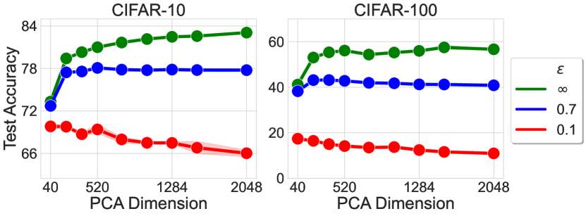
(b) MoCov2+ Pretraining

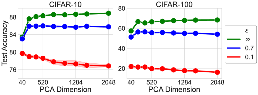
(c) SemiSL Pretraining

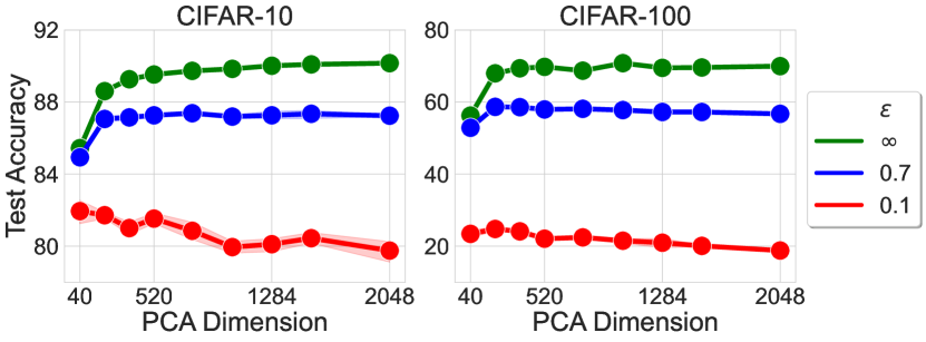
(d) SemiWeakSL Pretraining

Figure 8: DP Training of linear classifier on different pre-trained features using the PRV accountant for CIFAR-10 and CIFAR-100.

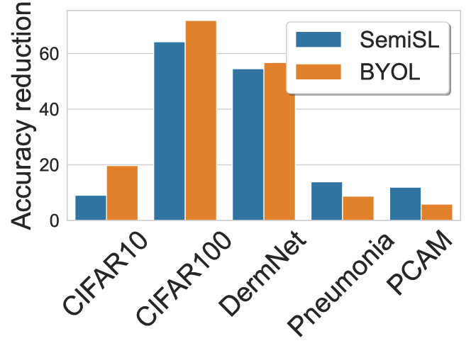
Figure 9: Comparing reduction in test accuracy for different datasets between using SemiSL and BYOL pre-trained networks.

In Figure 4 and 5 in the main text, we only reported accuracies for the best performing pre-training algorithm. In this, section we report the performance of our algorithm against five different pre-training algorithms that we consider in this paper. In particular, we consider two self-supervised pre-training algorithms: BYOL [Grill et al., 2020] and MoCov2+ [Chen et al., 2020] and two semi-supervised algorithms [Yalniz et al., 2019]. While one of them is a Semi-Supervised (SemiSL) algorithm, the other only uses weak supervision and we refer to it Semi-Weakly Supervised (SemiWeakSL) algorithm. In Figure 8 we report the results on CIFAR-10 and CIFAR-100. In Figure 10 we report the results for Flower-16 [Flo, 2021], GTSRB [Houben et al., 2013], PCAM [Veeling et al., 2018], Pneumonia [Kermany et al., 2018] and DermNet [Der, 2019].

Similar to Figure 6 in the main text, we show the accuracy reduction for Semi-Supervised pre-training vs BYOL (Self-Supervised) pre-trianing in Figure 9. Our results shows similar results as Shi et al. [2023] that labels are more useful for pre-training for tasks where there is a significant label overlap between the pre-training and the final task.

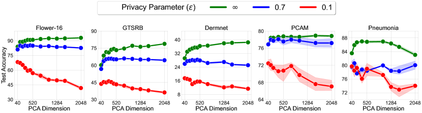
(a) SL Pretraining

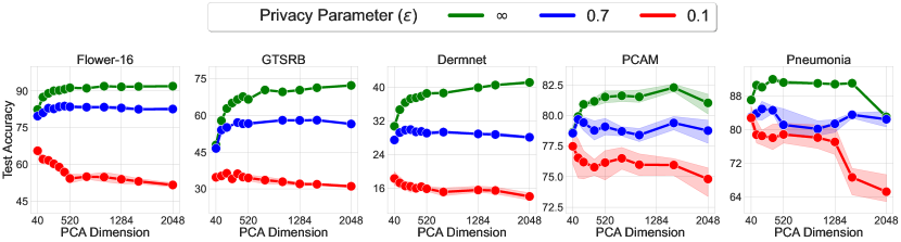
(b) BYOL Pretraining

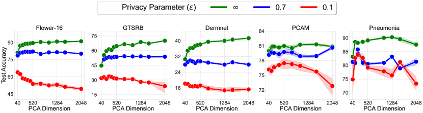
(c) MoCov2+ Pretraining

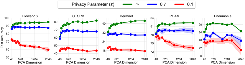
(d) SemiSL Pretraining

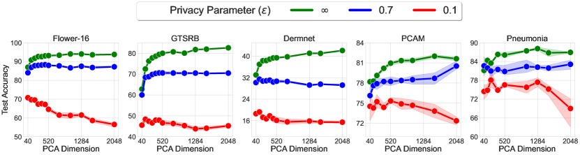
(e) SemiWeakSL Pretraining

Figure 10: DP Training of linear classifier on different pre-trained features using the PRV accountant for Flower-16, GTSRB, DermNet, PCAM, and Pneumonia.

Appendix C Computational Cost, Broader Impact and Limitations

Computational cost

Except for the supervised training on ImageNet32x32, we leverage pre-trained models. To optimize the training procedure, we checkpoint feature embeddings for each dataset and pre-trained model. Therefore, training requires loading the checkpoint and training a linear layer via SGD (or DP-SGD), accelerating the training procedure by avoiding the forward pass through the feature encoder. We use a single Tesla M40 (11GB) for each run. We perform approximately 405 runs for PILLAR. The same amount of runs is performed for the JL baseline. For GEP we perform 3528 runs. For AdaDPS we perform 4320 runs. We make the code needed to reproduce our main results available in the zip of the supplementary materials.

Broader impact and Limitations

In this work we show our method can be used in order to increase the utility of models under tight Differential Privacy constraints. Increasing the utility for low $\epsilon$ is crucial to foster the adoption of DP methods that provide provable guarantees for the privacy of users. Further, unlike several recent works that have shown improvement in accuracy for deep neural networks, our algorithm can be run on commonly available computational resources like a Tesla M40 11GB GPU as it does not require large batch sizes. We hope this will make DP training of high-performing deep neural networks more accessible. Finally, we show our algorithm improves not only on commonly used benchmarks like CIFAR10 and CIFAR100 but also in privacy relevant tasks like medical datasets including Pneumonia, PCAM, and DermNet. We hope this will encourage future works to also consider benchmarking their algorithms on more privacy relevant tasks.

As discussed, the assumption that labelled public data is available may not hold true in several applications. Our algorithm does not require the public data to be labelled, however the distribution shift between the public unlabelled data and the private one should not be too large. We have shown that for relatively small distribution shift our method remains effective. Finally, recent works have suggested that differentially private learning may disparately impact certain subgroups more than others [Bagdasaryan et al., 2019, Cummings et al., 2019, Sanyal et al., 2022]. It remains to explore whether semi-private learning can help alleviate these disparity.

References

- Shokri et al. (2017) Reza Shokri, Marco Stronati, Congzheng Song, and Vitaly Shmatikov. Membership inference attacks against machine learning models. In IEEE Symposium on Security and Privacy (SP), 2017.
- Ye et al. (2022) Jiayuan Ye, Aadyaa Maddi, Sasi Kumar Murakonda, Vincent Bindschaedler, and Reza Shokri. Enhanced membership inference attacks against machine learning models. In ACM SIGSAC Conference on Computer and Communications Security, 2022.
- Carlini et al. (2022) Nicholas Carlini, Steve Chien, Milad Nasar, Shuang Song, Andreas Terzis, and Florian Tramèr. Membership inference attacks from first principles. In IEEE Symposium on Security and Privacy (SP), 2022.
- Dwork et al. (2006) Cynthia Dwork, Frank McSherry, Kobbi Nissim, and Adam Smith. Calibrating noise to sensitivity in private data analysis. Theory of Cryptography, 2006.
- Kasiviswanathan et al. (2011) Shiva Prasad Kasiviswanathan, Homin K Lee, Kobbi Nissim, Sofya Raskhodnikova, and Adam Smith. What can we learn privately? SIAM Journal on Computing, 2011.
- Blum et al. (2005) Avrim Blum, Cynthia Dwork, Frank McSherry, and Kobbi Nissim. Practical privacy: the SuLQ framework. In ACM symposium on Principles of database systems, 2005.
- Beimel et al. (2013a) Amos Beimel, Kobbi Nissim, and Uri Stemmer. Characterizing the sample complexity of private learners. In Innovations in Theoretical Computer Science (ITCS), 2013a.
- Beimel et al. (2013b) Amos Beimel, Kobbi Nissim, and Uri Stemmer. Private learning and sanitization: Pure vs. approximate differential privacy. In Approximation, Randomization, and Combinatorial Optimization. Algorithms and Techniques, 2013b.
- Feldman and Xiao (2014) Vitaly Feldman and David Xiao. Sample complexity bounds on differentially private learning via communication complexity. In Conference on Learning Theory (COLT), 2014.
- Tramer and Boneh (2021) Florian Tramer and Dan Boneh. Differentially private learning needs better features (or much more data). In International Conference on Learning Representations (ICLR), 2021.
- De et al. (2022) Soham De, Leonard Berrada, Jamie Hayes, Samuel L Smith, and Borja Balle. Unlocking high-accuracy differentially private image classification through scale. arXiv:2204.13650, 2022.
- Li et al. (2022a) Xuechen Li, Florian Tramer, Percy Liang, and Tatsunori Hashimoto. Large language models can be strong differentially private learners. In International Conference on Learning Representations (ICLR), 2022a.
- Kurakin et al. (2022) Alexey Kurakin, Steve Chien, Shuang Song, Roxana Geambasu, Andreas Terzis, and Abhradeep Thakurta. Toward training at ImageNet scale with differential privacy. arXiv:2201.12328, 2022.
- Alon et al. (2019) Noga Alon, Raef Bassily, and Shay Moran. Limits of private learning with access to public data. In Conference on Neural Information Processing Systems (NeurIPS), 2019.
- Yu et al. (2021) Da Yu, Huishuai Zhang, Wei Chen, and Tie-Yan Liu. Do not let privacy overbill utility: Gradient embedding perturbation for private learning. In International Conference on Learning Representations (ICLR), 2021.
- Li et al. (2022b) Tian Li, Manzil Zaheer, Sashank Reddi, and Virginia Smith. Private adaptive optimization with side information. In International Conference on Machine Learning (ICML), 2022b.
- Papernot et al. (2017) Nicolas Papernot, Martín Abadi, Úlfar Erlingsson, Ian Goodfellow, and Kunal Talwar. Semi-supervised knowledge transfer for deep learning from private training data. In International Conference on Learning Representations (ICLR), 2017.
- Papernot et al. (2018) Nicolas Papernot, Shuang Song, Ilya Mironov, Ananth Raghunathan, Kunal Talwar, and Ulfar Erlingsson. Scalable private learning with PATE. In International Conference on Learning Representations (ICLR), 2018.
- Tramèr et al. (2022) Florian Tramèr, Gautam Kamath, and Nicholas Carlini. Considerations for differentially private learning with large-scale public pretraining. arXiv:2212.06470, 2022.
- Abadi et al. (2016) Martin Abadi, Andy Chu, Ian Goodfellow, H. Brendan McMahan, Ilya Mironov, Kunal Talwar, and Li Zhang. Deep learning with differential privacy. In ACM SIGSAC Conference on Computer and Communications Security, 2016.
- Li et al. (2022c) Xuechen Li, Daogao Liu, Tatsunori Hashimoto, Huseyin A Inan, Janardhan Kulkarni, YinTat Lee, and Abhradeep Guha Thakurta. When does differentially private learning not suffer in high dimensions? In Conference on Neural Information Processing Systems (NeurIPS), 2022c.
- Grill et al. (2020) Jean-Bastien Grill, Florian Strub, Florent Altché, Corentin Tallec, Pierre Richemond, Elena Buchatskaya, Carl Doersch, Bernardo Avila Pires, Zhaohan Guo, Mohammad Gheshlaghi Azar, et al. Bootstrap your own latent-a new approach to self-supervised learning. In Conference on Neural Information Processing Systems (NeurIPS), 2020.
- Deng et al. (2009) Jia Deng, Wei Dong, Richard Socher, Li-Jia Li, Kai Li, and Li Fei-Fei. ImageNet: A large-scale hierarchical image database. In IEEE Conference on Computer Vision and Pattern Recognition (CVPR), 2009.
- Chaudhuri et al. (2011) Kamalika Chaudhuri, Claire Monteleoni, and Anand D Sarwate. Differentially private empirical risk minimization. Journal of Machine Learning Research (JMLR), 2011.
- Bassily et al. (2014a) Raef Bassily, Adam Smith, and Abhradeep Thakurta. Private empirical risk minimization: Efficient algorithms and tight error bounds. In Annual Symposium on Foundations of Computer Science (FOCS), 2014a.
- Jensen et al. (2005) Carlos Jensen, Colin Potts, and Christian Jensen. Privacy practices of internet users: Self-reports versus observed behavior. International Journal of Human-Computer Studies, 2005.
- Chen et al. (2020) Xinlei Chen, Haoqi Fan, Ross Girshick, and Kaiming He. Improved baselines with momentum contrastive learning. arXiv:2003.04297, 2020.
- Yalniz et al. (2019) I. Zeki Yalniz, Hervé Jégou, Kan Chen, Manohar Paluri, and Dhruv Mahajan. Billion-scale semi-supervised learning for image classification. arxiv:1905.00546, 2019.
- Gu et al. (2023) Xin Gu, Gautam Kamath, and Zhiwei Steven Wu. Choosing public datasets for private machine learning via gradient subspace distance. arXiv:2303.01256, 2023.
- Bassily et al. (2014b) Raef Bassily, Adam D. Smith, and Abhradeep Thakurta. Private empirical risk minimization, revisited. ICML Workshop on Learning, Security and Privacy, 2014b.
- McSherry and Talwar (2007) Frank McSherry and Kunal Talwar. Mechanism design via differential privacy. In Annual Symposium on Foundations of Computer Science (FOCS), 2007.
- Nguyen et al. (2020) Huy Le Nguyen, Jonathan R. Ullman, and Lydia Zakynthinou. Efficient private algorithms for learning large-margin halfspaces. In Algorithmic Learning Theory (ALT), 2020.
- Blum and Roth (2013) Avrim Blum and Aaron Roth. Fast private data release algorithms for sparse queries. In Approximation, Randomization, and Combinatorial Optimization., 2013.
- Donhauser et al. (2023) Konstantin Donhauser, Johan Lokna, Amartya Sanyal, March Boedihardjo, Robert Hönig, and Fanny Yang. Sample-efficient private data release for lipschitz functions under sparsity assumptions. arXiv:2302.09680, 2023.
- Zhou et al. (2021) Yingxue Zhou, Steven Wu, and Arindam Banerjee. Bypassing the ambient dimension: Private SGD with gradient subspace identification. In International Conference on Learning Representations (ICLR), 2021.
- Kasiviswanathan (2021) Shiva Prasad Kasiviswanathan. SGD with low-dimensional gradients with applications to private and distributed learning. In Proceedings of the Conference on Uncertainty in Artificial Intelligence (UAI), 2021.
- Bun et al. (2020) Mark Bun, Marco Leandro Carmosino, and Jessica Sorrell. Efficient, noise-tolerant, and private learning via boosting. In Conference on Learning Theory (COLT), 2020.
- Awasthi et al. (2020) Pranjal Awasthi, Natalie Frank, and Mehryar Mohri. On the Rademacher complexity of linear hypothesis sets. arXiv:2007.11045, 2020.
- Krizhevsky (2009) Alex Krizhevsky. Learning multiple layers of features from tiny images, 2009. URL http://www.cs.toronto.edu/~kriz/cifar.html.
- Dwork (2011) Cynthia Dwork. A firm foundation for private data analysis. Communications of the ACM, 2011.
- Yeom et al. (2018) Samuel Yeom, Irene Giacomelli, Matt Fredrikson, and Somesh Jha. Privacy risk in machine learning: Analyzing the connection to overfitting. In IEEE computer security foundations symposium (CSF), 2018.
- Nasr et al. (2021) Milad Nasr, Shuang Songi, Abhradeep Thakurta, Nicolas Papemoti, and Nicholas Carlin. Adversary instantiation: Lower bounds for differentially private machine learning. In IEEE Symposium on Security and Privacy (SP), 2021.
- Mironov (2017) Ilya Mironov. Rényi differential privacy. In IEEE computer security foundations symposium (CSF), 2017.
- Gopi et al. (2021a) Sivakanth Gopi, Yin Tat Lee, and Lukas Wutschitz. Numerical composition of differential privacy. In A. Beygelzimer, Y. Dauphin, P. Liang, and J. Wortman Vaughan, editors, Conference on Neural Information Processing Systems (NeurIPS), 2021a.
- Flo (2021) Flowers dataset. https://tinyurl.com/2p8vpsp2, 2021.
- Houben et al. (2013) Sebastian Houben, Johannes Stallkamp, Jan Salmen, Marc Schlipsing, and Christian Igel. Detection of traffic signs in real-world images: The German Traffic Sign Detection Benchmark. In International Joint Conference on Neural Networks, 2013.
- Kermany et al. (2018) Daniel S Kermany, Michael Goldbaum, Wenjia Cai, Carolina CS Valentim, Huiying Liang, Sally L Baxter, Alex McKeown, Ge Yang, Xiaokang Wu, Fangbing Yan, et al. Identifying medical diagnoses and treatable diseases by image-based deep learning. cell, 2018.
- Veeling et al. (2018) Bastiaan S Veeling, Jasper Linmans, Jim Winkens, Taco Cohen, and Max Welling. Rotation equivariant CNNs for digital pathology. arXiv:1806.03962, 2018.
- Der (2019) Dataset for 23 skin lesions. https://www.kaggle.com/datasets/shubhamgoel27/dermnet, 2019.
- Shi et al. (2023) Yuge Shi, Imant Daunhawer, Julia E. Vogt, Philip H.S. Torr, and Amartya Sanyal. How robust are pre-trained models to distribution shift? In International Conference on Learning Representations (ICLR), 2023.
- Recht et al. (2018) Benjamin Recht, Rebecca Roelofs, Ludwig Schmidt, and Vaishaal Shankar. Do CIFAR-10 classifiers generalize to CIFAR-10? arxiv:1806.00451, 2018.
- Zwald and Blanchard (2005) Laurent Zwald and Gilles Blanchard. On the convergence of eigenspaces in kernel principal component analysis. In Conference on Neural Information Processing Systems (NeurIPS), 2005.
- Anthony and Bartlett (1999) Martin Anthony and Peter L. Bartlett. Neural Network Learning: Theoretical Foundations. Cambridge University Press, 1999.
- Vershynin (2018) Roman Vershynin. High-Dimensional Probability: An Introduction with Applications in Data Science. Cambridge University Press, 2018.
- Gharan (2017) Shayan Oveis Gharan. Low rank approximation. Lecture notes for CSE 521: Design and Analysis of Algorithms I, 2017.
- Yousefpour et al. (2021) Ashkan Yousefpour, Igor Shilov, Alexandre Sablayrolles, Davide Testuggine, Karthik Prasad, Mani Malek, John Nguyen, Sayan Ghosh, Akash Bharadwaj, Jessica Zhao, Graham Cormode, and Ilya Mironov. Opacus: User-friendly differential privacy library in PyTorch. arXiv:2109.12298, 2021.
- Wightman (2019) Ross Wightman. Pytorch image models. https://github.com/rwightman/pytorch-image-models, 2019.
- da Costa et al. (2022) Victor Guilherme Turrisi da Costa, Enrico Fini, Moin Nabi, Nicu Sebe, and Elisa Ricci. solo-learn: A library of self-supervised methods for visual representation learning. Journal of Machine Learning Research (JMLR), 2022.
- Zhu et al. (2020) Yuqing Zhu, Xiang Yu, Manmohan Chandraker, and Yu-Xiang Wang. Private-knn: Practical differential privacy for computer vision. In IEEE Conference on Computer Vision and Pattern Recognition (CVPR), 2020.
- Mühl and Boenisch (2022) Christopher Mühl and Franziska Boenisch. Personalized PATE: Differential privacy for machine learning with individual privacy guarantees. In Proceedings on Privacy Enhancing Technologies (PoPETS), 2022.
- Boenisch et al. (2023) Franziska Boenisch, Christopher Mühl, Adam Dziedzic, Roy Rinberg, and Nicolas Papernot. Have it your way: Individualized privacy assignment for DP-SGD. arXiv:2303.17046, 2023.
- Gopi et al. (2021b) Sivakanth Gopi, Yin Tat Lee, and Lukas Wutschitz. Numerical composition of differential privacy. In Conference on Neural Information Processing Systems (NeurIPS), 2021b.
- Johnson (1984) William B. Johnson. Extensions of lipschitz mappings into hilbert space. Contemporary Mathematics, 1984.
- Bagdasaryan et al. (2019) Eugene Bagdasaryan, Omid Poursaeed, and Vitaly Shmatikov. Differential privacy has disparate impact on model accuracy. In Conference on Neural Information Processing Systems (NeurIPS), 2019.
- Cummings et al. (2019) Rachel Cummings, Varun Gupta, Dhamma Kimpara, and Jamie Morgenstern. On the compatibility of privacy and fairness. In Conference on User Modeling, Adaptation and Personalization, 2019.
- Sanyal et al. (2022) Amartya Sanyal, Yaxi Hu, and Fanny Yang. How unfair is private learning? In Proceedings of the Conference on Uncertainty in Artificial Intelligence (UAI), 2022.