The Formation of Magellanic System and the total mass of Large Magellanic Cloud

Abstract

The Magellanic Stream is unique to sample the MW potential from $\sim$50 kpc to 300 kpc, and is also unique in constraining the LMC mass, an increasingly important question for the Local Group/Milky Way modeling. Here we compare strengths and weaknesses of the two types of models (tidal and ram-pressure) of the Magellanic Stream formation. I will present our modeling for the formation of the Magellanic System, including those of the most recent discoveries in the Stream, in the Bridge and at the outskirts of Magellanic Clouds. This model has been successful in predicting most recent observations in both properties of stellar and gas phase. It appears that it is an over-constrained model and provides a good path to investigate the Stream properties. In particular, this model requires a LMC mass significantly smaller than 10¹¹ M_⊙.

1 Introduction

The Magellanic Stream (MS) and Leading Arm (LA) subtend an angle of 230^∘, which is identified to be anchored to the Magellanic Clouds in 1974 by Mathewson, Cleary & Murray (1974). The nature of its formation was considered still unknown in 2012 (Mathewson, 2012). Modern observations of proper motion from both HST and GAIA are indicating that the the Clouds are presently at first passage to the Milky Way (Kallivayalil et al., 2006; Piatek, Pryor & Olszewski, 2008; Kallivayalil et al., 2013). Besides large amount of neutral gas distributed along the Stream, there are mounting evidence that 3-4 times more ionized than neutral gas has been deposited along the Stream (Fox et al., 2014; Richter et al., 2017).

In the first infall frame, the explanations of the MS can be broadly classified into two schemes. One is the tidal tail model (Besla et al., 2012; Lucchini et al., 2020), the other is ram-pressure tails (Mastropietro, 2010; Hammer et al., 2015; Wang et al., 2019; Wang, Hammer & Yang, 2022). In the tidal tail model, the MS is generated by the mutual close interaction 1-2 Gyr ago before the MCs entering into the halo of MW. In this scenario, the SMC is assumed to be a long-lived satellite of LMC, which requires a LMC mass in excess of 10¹¹ M_⊙.

There are several major limitations for the tidal model. First, it already lacks by a factor of 10 the amount of neutral gas observed in the Stream. Second, it is unable to reproduce the huge amount of ionized gas that is observed along the Stream. Third, it can only produce a single stream filament, while the MS are made of two filaments, which have been clearly identified by chemical, kinematic, and morphological analyses (Nidever et al., 2010; Hammer et al., 2015). Fourth, no stars along the stream have been observed. Recent revised tidal model have been made by including hot corona of LMC to amend parts of above drawbacks (Lucchini et al., 2020; Lucchini, D’Onghia & Fox, 2021). But these models required either a unreasonable massive corona of LMC that is even larger than that of MW, or a dramatic change of the Cloud orbits, which can not reproduce their observed proper motions within $3\sigma$.

Conversely to the tidal model, the ram-pressure plus collision model (Hammer et al., 2015; Wang et al., 2019) naturally reproduce most observational properties associated with the Magellanic System, for instance, the dual filaments, huge amount of ionized gas, absence of stars in the Stream. Interestingly, several observations made after the elaboration of the model have been reproduced without fine tuning.

In this scenario, the Leading Arm are the trailing gas of front-runner dwarfs (Yang et al., 2014; Hammer et al., 2015; Tepper-García et al., 2019), which is well supported by the determination of low metal abundances in 3 part of this structure (see Philip Richter’s contribution).

2 Two hydrodynamic filaments formed by ram-pressure plus collision

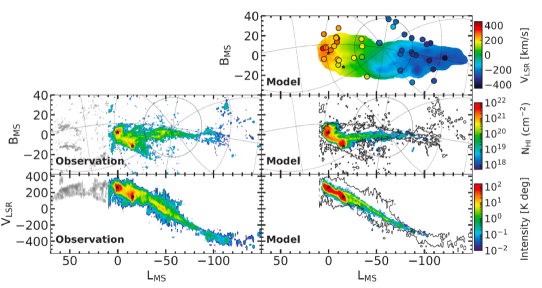
Figure 1: Comparing HI and ionized gas from simulation model (right panels) from Wang et al. (2019) with observations (left panels) of Nidever et al. (2010). The top-right panel shows the sky distribution of the simulated ionized gas with a color coding for the line-of-sight velocity. Circle points represent QSOs absorption line observations by HST/COS (Fox et al., 2014). The simulated ionized gas mass is consistent with that observed (D’Onghia & Fox, 2016). The bottom two rows compare observed HI distributions of the Magellanic Stream with that of simulations. The black stars in each panel indicate the position of LMC and SMC. In the simulation panels the contours indicates the observations data. The LA is assumed to have another origin rather than the MC gas (Yang et al., 2014; Hammer et al., 2015; Tepper-García et al., 2019).

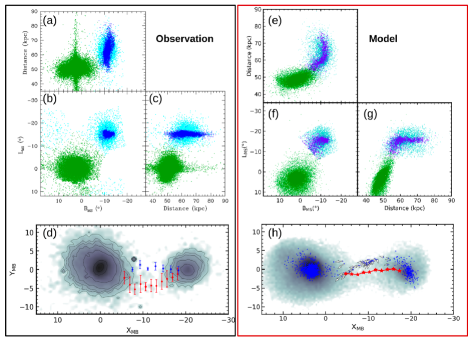
Figure 2: Comparing the stellar distribution of MCs between simulation model from Wang et al. (2019) (the right-hand panels enclosed within rectangle a red box ) and observation data (the right-hand panels enclosed within a black box). In the observation panels (a,b,c), the green and cyan points represent ancient RR Lyrae stars from LMC and SMC, and blue points indicates the Classical Cepheids (Ripepi et al., 2017). In the simulation panels, particle numbers and sky distribution have been selected following the observations. The simulation model reproduces well the ’cigar’ shape of SMC. Panel d shows the ancient star distribution on the sky, overlapping in the Bridge region RR Lyrae stars and young main sequence stars from Belokurov et al. (2017). Panel h shows simulation model from Wang et al. (2019) which show a similar offset of young stars with ancient stars in the Bridge region.

In the frame of the ram-pressure and collision model, we have built a stable model of Milky Way which include a hot gas corona. The progenitors of MCs are gas rich dwarf galaxies before entering the halo of MW. Figure 1 compare the observed neutral gas and ionized gas to this model. This model naturally generates two HI streams behind the MCs, and a huge amount of ionized gas deposited along the stream. The strong mutual interaction between the MCs totally stretched by gravitational tides the SMC into a ’cigar’ shape, which is well reproduced by this model as shown in Figure 2. Recent observation indicates that there is offset between the ancient stars and young stellar population in the Bridge region (Belokurov et al., 2017), which is also well reproduced in this model.

3 Many Predictions Are Confirmed by Observations

With the progress of observations, new data and findings provide essential test for any model aiming at reproducing the formation of Magellanic System. We will show that our ram-pressure plus collision model pass these tests with many predictions confirmed by recent observations.

3.1 Two separated populations in the Bridge region

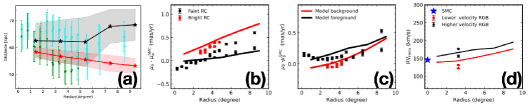
Figure 3: Comparing the observed distances (panel a), relative proper motion (panel b, c), and line-of-sight velocity (panel d) of foreground and background stellar population in the Bridge region as function radius to SMC between observation data and simulation model. In panel a, the green and cyan color points indicate bright and faint population of red clump stars from Omkumar et al. (2021) for north-east (solid square) and south-east region (open square). The proper motion of faint (black square) and bright (red square) RC in the left-hand and middle panel are from Omkumar et al. (2021). The radial velocity of the lower (red circles) and higher (black circles) velocity RGB stars are from James et al. (2021), which are corresponds to foreground components and main body of SMC. The blue star in the panel d indicates the SMC value. The observed proper motions and radial velocity of SMC are from Zivick et al. (2018).

Observations indicate that there are two different populations in the Bridge region, which are separated in both distance and kinematics space (e.g., Omkumar et al., 2021; James et al., 2021). Omkumar et al. (2021) found that two populations of red clump stars in the Bridge region starting from SMC to LMC, which show different brightnesses. The bright and faint red clump populations show different distance and kinematics, which consistent with the finding of James et al. (2021). In our model, the two populations are formed by SMC, which are tidally stripped by the LMC. The foreground population indicates the disk component of SMC, which is tidally stripped from SMC and showing debris of interaction stretching from SMC to LMC. While the background population come from the spheroid component which is less affected by the LMC tidal and distributed in the back of the Bridge region. This model naturally reproduces this new observation as shown in Figure 3.

3.2 Periphery of the Clouds

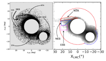
Figure 4: Comparing the morphology of MCs with Gaia EDR3 data (Gaia Collaboration et al., 2021) with simulation model (Wang, Hammer & Yang, 2022). In the right panel, the red and blue dashed line indicate the sample selection region for Gaia data (Gaia Collaboration et al., 2021). In the right-hand panel, the colored polygon regions indicate different substructures associated with LMC detected by Gatto et al. (2022).

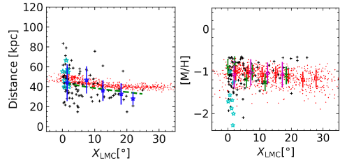
Figure 5: The distance and metallicity of NTA stars varied with X_LMC. The black crosses are selected with Gaia EDR3 (Gaia Collaboration et al., 2021) and StarHorse (Anders et al., 2022) (see the text for details), and the red points indicates data from our simulation model. The cyan stars indicate the data from Huang et al. (2022), who derived star distance and metallicity from SkyMapper DR2 (Onken et al., 2019) and Gaia EDR3. The blue stars and its associated error bars in the left panel indicate the mean and dispersion for the observed stars. The green line in the left panel denotes an inclined disk following van der Marel & Kallivayalil (2014). In the right panel, the magenta squares and its associated error bars show the mean and dispersion of observation data from Grady, Belokurov & Evans (2021). The green stars and its associated error bars indicate the value from observation data of MagES (Cullinane et al., 2022a). The red squares and its associated error bars are the mean and dispersion value of simulation model.

With deep observations, many faint features in the periphery of MCs have been discovered as shown in the left panel of Figure 4 from Gaia Collaboration et al. (2021), many of which have been well predicted by our model as shown in the right panel of Figure 4. The North Tidal Arm (NTA) is the largest tidal features rooted from the disk LMC, which is confirmed to originate from the LMC on the basis of its metallicity, distance, and kinematics (Cullinane et al., 2022a, b, 2020). Before observations, the model of Wang et al. (2019) predicted the existence of the NTA , which is formed by the Galactic tides exerted on the disk of LMC.

From Gaia EDR3, we have selected stars belonging to NTA according to its morphology position, proper motion. With this sample stars of NTA, we cross-matched with results of literature to get their distance and metallicity. The distance and metallicity variation as function of radius to the LMC are shown in Figure 5.

In order to compare simulation model with observations, we assigned metallicities to particles of the simulation model by painting that of the LMC with metallicities following the observational constraints (Grady, Belokurov & Evans, 2021). Grady, Belokurov & Evans (2021) selected red giant stars of LMC from Gaia DR2, and used machine-learning method with data of Gaia+2MASS+WISE to estimate the photometric metallicity for these stars. With these data set, they estimated radial metallicity profile: [Fe/H] = $\alpha$ R + $b$. They found the $\alpha=-0.048\pm 0.001$ dex kpc^-1 and $b=-0.656\pm 0.004$ dex. We use this relation to paint the initial metallicity of our modeled LMC. For simplicity, we have adopted the approximated relation [Fe/H] $\sim$ [M/H]. In Figure 5, the modeled data are shown with red points. The simulation model, can explain well the observational results for both the distance and metallicity profiles, without fine tuning. The current observed metallicity profile of the LMC (Grady, Belokurov & Evans, 2021) also reproduces the formation of NTA, which indicates that the LMC metallicity profile has been settled down before the formation of NTA, or the mutual interaction of MCs/gas loss have marginal influence on the metallicity structure of LMC.

4 Conclusion

The ram-pressure plus collision model (Hammer et al., 2015; Wang et al., 2019) can not only reproduce MS, but also succeed in predicting many observations that have been done in the meantime (see a description in Wang, Hammer & Yang 2022). This model naturally reproduces the two inter-twisted filaments of HI MS, as well as the huge amount of ionized gas associated with MS. This ability also validates that this model goes into the right direction to disentangle the mystery of Magellanic System formation (Mathewson, private communication). We conjecture that the LMC mass has to be small (a few times 10¹⁰ M_⊙) to form the Magellanic Stream, though further studies are needed to explore the exact mass range.

Müller OliverDo you think we can find other dwarfs showing ’cigar’ shape as SMC in the extragalactic dwarfs ? Jianling WANGThis is difficult, since we need precise distance for individual star showing dwarf shapes in 3D.

References

- Anders et al. (2022) Anders F. et al., 2022, A&A, 658, A91
- Belokurov et al. (2017) Belokurov V., Erkal D., Deason A. J., Koposov S. E., De Angeli F., Evans D. W., Fraternali F., Mackey D., 2017, MNRAS, 466, 4711
- Besla et al. (2012) Besla G., Kallivayalil N., Hernquist L., van der Marel R. P., Cox T. J., Kereš D., 2012, MNRAS, 421, 2109
- Cullinane et al. (2022a) Cullinane L. R., Mackey A. D., Da Costa G. S., Erkal D., Koposov S. E., Belokurov V., 2022a, MNRAS, 510, 445
- Cullinane et al. (2022b) Cullinane L. R., Mackey A. D., Da Costa G. S., Erkal D., Koposov S. E., Belokurov V., 2022b, MNRAS, 512, 4798
- Cullinane et al. (2020) Cullinane L. R. et al., 2020, MNRAS, 497, 3055
- D’Onghia & Fox (2016) D’Onghia E., Fox A. J., 2016, ARA&A, 54, 363
- Fox et al. (2014) Fox A. J. et al., 2014, ApJ, 787, 147
- Gatto et al. (2022) Gatto M., Ripepi V., Bellazzini M., Tortora C., Tosi M., Cignoni M., Longo G., 2022, ApJ, 931, 19
- Gaia Collaboration et al. (2021) Gaia Collaboration et al., 2021, A&A, 649, A7
- Grady, Belokurov & Evans (2021) Grady J., Belokurov V., Evans N. W., 2021, ApJ, 909, 150
- Hammer et al. (2015) Hammer F., Yang Y. B., Flores H., Puech M., Fouquet S., 2015, ApJ, 813, 110
- Huang et al. (2022) Huang Y. et al., 2022, ApJ, 925, 164
- James et al. (2021) James D. et al., 2021, MNRAS, 508, 5854
- Kallivayalil et al. (2006) Kallivayalil N., van der Marel R. P., Alcock C., Axelrod T., Cook K. H., Drake A. J., Geha M., 2006, The Astrophysical Journal, 638, 772
- Kallivayalil et al. (2013) Kallivayalil N., van der Marel R. P., Besla G., Anderson J., Alcock C., 2013, The Astrophysical Journal, 764, 161
- Lucchini et al. (2020) Lucchini S., D’Onghia E., Fox A. J., Bustard C., Bland-Hawthorn J., Zweibel E., 2020, Nature, 585, 203
- Lucchini, D’Onghia & Fox (2021) Lucchini S., D’Onghia E., Fox A. J., 2021, ApJL, 921, L36
- Mastropietro (2010) Mastropietro C., 2010, in American Institute of Physics Conference Series, Vol. 1240, Hunting for the Dark: the Hidden Side of Galaxy Formation, Debattista V. P., Popescu C. C., eds., pp. 150–153
- Mathewson (2012) Mathewson D., 2012, Journal of Astronomical History and Heritage, 15, 100
- Mathewson, Cleary & Murray (1974) Mathewson D. S., Cleary M. N., Murray J. D., 1974, The Astrophysical Journal, 190, 291
- Nidever et al. (2010) Nidever D. L., Majewski S. R., Butler Burton W., Nigra L., 2010, ApJ, 723, 1618
- Omkumar et al. (2021) Omkumar A. O. et al., 2021, MNRAS, 500, 2757
- Onken et al. (2019) Onken C. A. et al., 2019, PASA, 36, e033
- Piatek, Pryor & Olszewski (2008) Piatek S., Pryor C., Olszewski E. W., 2008, The Astronomical Journal, 135, 1024
- Richter et al. (2017) Richter P. et al., 2017, A&A, 607, A48
- Ripepi et al. (2017) Ripepi V. et al., 2017, MNRAS, 472, 808
- Tepper-García et al. (2019) Tepper-García T., Bland-Hawthorn J., Pawlowski M. S., Fritz T. K., 2019, MNRAS, 488, 918
- van der Marel & Kallivayalil (2014) van der Marel R. P., Kallivayalil N., 2014, ApJ, 781, 121
- Wang et al. (2019) Wang J., Hammer F., Yang Y., Ripepi V., Cioni M.-R. L., Puech M., Flores H., 2019, MNRAS, 486, 5907
- Wang, Hammer & Yang (2022) Wang J., Hammer F., Yang Y., 2022, MNRAS, 515, 940
- Yang et al. (2014) Yang Y., Hammer F., Fouquet S., Flores H., Puech M., Pawlowski M. S., Kroupa P., 2014, MNRAS, 442, 2419
- Zivick et al. (2018) Zivick P. et al., 2018, ApJ, 864, 55