Inferring interpretable dynamical generators of local quantum observables from projective measurements through machine learning

Abstract

To characterize the dynamical behavior of many-body quantum systems, one is usually interested in the evolution of so-called order-parameters rather than in characterizing the full quantum state. In many situations, these quantities coincide with the expectation value of local observables, such as the magnetization or the particle density. In experiment, however, these expectation values can only be obtained with a finite degree of accuracy due to the effects of the projection noise. Here, we utilize a machine-learning approach to infer the dynamical generator governing the evolution of local observables in a many-body system from noisy data. To benchmark our method, we consider a variant of the quantum Ising model and generate synthetic experimental data, containing the results of $N$ projective measurements at $M$ sampling points in time, using the time-evolving block-decimation algorithm. As we show, across a wide range of parameters the dynamical generator of local observables can be approximated by a Markovian quantum master equation. Our method is not only useful for extracting effective dynamical generators from many-body systems, but may also be applied for inferring decoherence mechanisms of quantum simulation and computing platforms.

Introduction.—

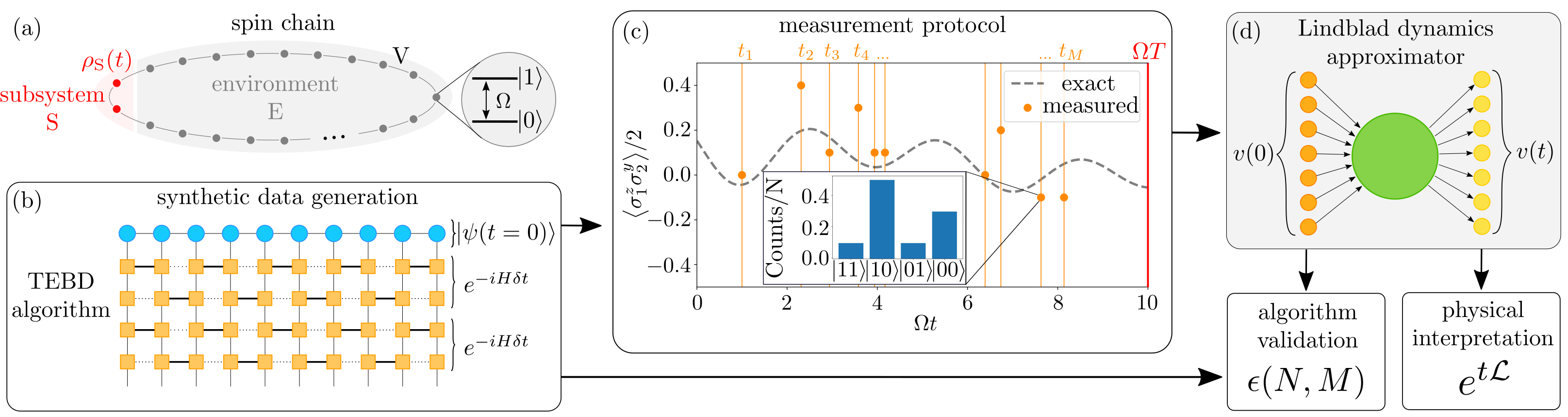
Figure 1: System and measurement protocol. (a) The system is composed of the two-spin subsystem S, which is embedded in the environment E consisting of $L-2$ spins. The Hamiltonian describing the system [cf. Eq. (1)] features a driving field with Rabi frequency $\Omega$ and nearest-neighbor interactions with coupling strength $V$. (b) Synthetic data generation using the time-evolving block-decimation algorithm. The time evolution operator is approximated using Trotterization: $U_{t}=e^{-iHt}\approx\prod e^{-iH\delta t}$. The time evolution is then obtained by repeatedly applying $e^{-iH\delta t}$. (c) Sketch of the measurement protocol. The gray dashed line represents the exact dynamics of the observable. For each trajectory, $M$ random points are selected in the time window $[0,\Omega T]$ (here $\Omega T=10$). For each point in time, we measure $N$ times in a suitable basis; here $z$/$y$-basis for the first/second spin. The inset shows an example histogram of measurement outcomes: $\ket{10}$ means the measurement on the first spin along $z$-basis has outcome $1$, and the measurement on the second spin along $y$-basis has outcome $0$. From the histogram, the expectation value depicted as orange dots are obtained. (d) The synthetic data is fed to the ML algorithm, namely a single layer perceptron, that learns the dynamical generator $\mathcal{L}$. The algorithm is validated by comparison to the exact data, where the error $\epsilon(N,M)$ is calculated for different values of $N$ and $M$. The ML method is interpretable and can be used to “read out” the underlying dynamical processes.

Reconstructing Hamiltonian operators or dynamical generators from physical properties of a quantum system is a problem of current interest. For instance, inverse methods can be applied to identify quantum Hamiltonians associated with a given ground state [1] and interacting many-body theories can be obtained from the knowledge of correlation functions [2, 3]. In many settings, one is merely interested in reconstructing effective equations of motion for a subsystem S embedded in a larger “environment” E, as it happens, for open quantum systems [4, 5, 6, 7, 8]. Furthermore, in the framework of quantum simulation [9, 10, 11, 12, 13, 14, 15, 16, 17], it is very important to understand the (effective) dynamical equations under which artificial quantum systems actually evolve and by how much these differ from the desired ones [18, 19]. This is relevant for improving state-of-the-art hardware [20, 21] and the identification of noise models. Another interesting instance concerns the evolution of order parameters, often constructed from local observables, such as the particle density or the magnetization.

Machine learning (ML) approaches appear to be particularly suited for this task [22]. For instance, quantum process tomography with generative adversarial methods [23], neural networks [24], and recurrent neural networks [25, 26] have been developed. These approaches are very promising but have two main drawbacks: they require a great number of measurements, and they treat ML algorithms as black boxes, thus lacking in physical interpretation. Simpler methods are capable of learning Hamiltonians from fewer local measurements [27, 28, 29, 30, 31, 32, 33], yet they typically rely on a a priori ansatz for the functional form of the Hamiltonian or of the dissipation. A more general approach is to fit an open quantum system (OQS) dynamics by learning the Nakajima-Zwanzig equation [34, 35] through transfer tensor techniques [36, 37, 38] or by learning convolutionless master equations [39]. However, these approaches require a full state tomography at different time steps, which is prohibitive to achieve in experiments. Ultimately, current methods thus either rely on an ad hoc ansatz, or demand data which is not experimentally accessible, or lack in physical interpretability (which is actually becoming highly desirable [40]).

In this work, we show how to use ML methods to infer the effective dynamical generator of a subsystem from a finite set of local measurements at randomly selected times, which inevitably produce noisy data due to projection noise. To illustrate our approach, we consider a many-body spin system [cf. Fig. 1(a)], which is ubiquitous in the context of experiments with trapped ion or Rydberg atom quantum simulators [21, 41, 42]. By using synthetic (experimental) data generated by tensor-network based algorithms we infer a physically consistent Markovian dynamical generator [43, 44] governing the evolution of a small subsystem. Our method, which works reliably across a wide range of parameters – even in some instances outside the weak coupling limit – yields interpretable results which may be used to infer noise models on quantum simulators or to study thermalization dynamics in many-body systems.

Setting.— The system we consider is a $1D$ quantum spin chain consisting of $L$ spins arranged on a circular lattice, as depicted in Fig. 1(a). The chain is partitioned into a subsystem S, here formed by two adjacent spins, and the environment E, that is, the remainder of the spin chain. We assume the whole system to evolve unitarily, through the many-body Hamiltonian

$$H_{S+E}=\frac{\Omega}{2}\sum_{i=1}^{L}\sigma_{i}^{x}+V\bigg{(}\sum_{i=1}^{L-1}n_{i}n_{i+1}+n_{L}n_{1}\bigg{)}\,.$$ (1)

The first term in the equation above describes a transverse “laser” field, while the second one accounts for nearest-neighbor interactions. Here, $\sigma_{i}^{\alpha}$ denotes the $\alpha$ Pauli matrix for the $i^{th}$ spin and we have defined the projector $n=\frac{1+\sigma^{z}}{2}$. The above Hamiltonian is of practical interest for experiments with Rydberg atoms [42] and essentially encodes an Ising model in the presence of transverse and longitudinal fields. We simulate the time evolution of the whole system by means of the time-evolving block-decimation (TEBD) algorithm [see Fig. 1(b)].

In our setting, the information on the state of S is obtained by a finite number, $N$, of projective measurements, taken at randomly selected times $t_{1},...\,t_{M}$ [see Fig. 1(c)]. From this noisy data we want to infer the open quantum dynamics of the reduced state $\rho_{\mathrm{S}}(t)$ of subsystem S. Formally, this dynamics is obtained as the partial trace of the evolution of the full many-body state, i.e., $\rho_{\mathrm{S}}(t)={\rm Tr}_{\mathrm{E}}\left(U_{t}\rho_{\mathrm{S+E}}U_{t}^{\dagger}\right)$, where $U_{t}=e^{-iHt}$, $\rho_{\mathrm{S+E}}$ is the initial state of the system and ${\rm Tr}_{E}$ denotes the trace over the environment degrees of freedom. In general, such a dynamics is rather involved and may show non-Markovian effects or it may be nonlinear for generic initial states $\rho_{\mathrm{S+E}}$ [45]. Here, we restrict ourselves to learning a Markovian dynamics for $\rho_{\mathrm{S}}(t)$, but more general approaches are certainly possible [43]. The goal is then to identify the time-independent generator $\mathcal{L}$, yielding the Markovian quantum master equation evolution [45, 46, 47],

$$\dot{\rho}_{S}(t)=\mathcal{L}[\rho_{S}(t)]$$ (2)

that optimally describes the dynamics of S. This simple form has the advantage that it is straightforwardly interpretable, i.e., it allows to read off the Hamiltonian and decoherence processes (see further below).

Data generation.— We simulate the time evolution of the system for times $t\in[0,\Omega T]$ by means of matrix product states and the time-evolving block-decimation algorithm [48, 49, 50] [see Fig. 1(b)], which allows us to study systems of up to $50$ spins. We generate $30$ trajectories obtained by initializing the system in state $\psi=\bigotimes_{k=1}^{L}\ket{0}$, with $\sigma^{z}\ket{0}=-\ket{0}$ and perturbing the subsystem S through a random two-spin unitary $\hat{U}_{\mathrm{rand}}$ distributed with the Haar measure. As the system evolves in time, after each time-step $\Omega dt=0.01$, we calculate the expectation value of all the $15$ independent observables $\{\mathds{1}_{1}\otimes\sigma_{2}^{x},\mathds{1}_{1}\otimes\sigma_{2}^{y},...,\sigma_{1}^{x}\otimes\sigma_{2}^{y},...,\sigma_{1}^{z}\otimes\sigma_{2}^{z}\}/2$ of the subsystem S, which uniquely identify the reduced subsystem state. With the reduced state at hand, we can emulate experimental measurements of the above local observables. For each trajectory, we select $M$ random times in the time-window $[0,\Omega T]$ and, for each of these points in time, we perform $N$ measurements in all the relevant basis in order to produce a noisy estimate of the reduced state. Such a procedure is sketched in Fig. 1(c), in which the histogram depicts the counting of $N=10$ measurement outcomes for a single time-point, whereas the orange dots represent the experimental expectation value.

ML architecture and training.— The generator $\mathcal{L}$ defining the quantum master equation (2) can be parametrized as $\mathcal{L}=\mathcal{H}+\mathcal{D}$, where

$$\mathcal{H}[\cdot] =-i[H,\cdot]\,,\quad\mbox{with}\quad H=\sum_{i=2}^{d^{2}}\theta^{H}_{i}F_{i}\,,$$ (3)

$$\mathcal{D}[\cdot] =\frac{1}{2}\sum_{i,j=2}^{d^{2}}c_{ij}([F_{i},\cdot F^{\dagger}_{j}]+[F_{i}\cdot,F^{\dagger}_{j}])\,.$$

Here, we have introduced the Hermitian orthonormal basis $\{F_{i}\}_{i=1}^{16}$, for the operators of the subsystem S. Note that we choose $F_{1}$ to be proportional to the identity operator, specifically $F_{1}=\mathds{1}/\sqrt{d}$. Moreover, we write the Hamiltonian in terms of the “fields” $\theta^{H}_{i}$, and the dissipative contribution $\mathcal{D}$ in a non-diagonal form, fully specified by the so-called Kossakowski matrix $c_{ij}$. The latter must be positive semi-definite in order for the open quantum dynamics to be completely positive. This constraint can be “hard coded” by setting $c=Z^{\dagger}Z$, for a complex matrix $Z=\theta^{X}+i\theta^{Y}$, with $\theta^{X}$ and $\theta^{Y}$ being real-valued.

In the same spirit, we decompose the reduced state $\rho_{S}$ on the basis $\{F_{i}\}_{i=1}^{16}$ as [51]

$$\rho_{\mathrm{S}}=\frac{\mathds{1}}{d}+\sum_{i=2}^{16}F_{i}v_{i}\,,$$ (4)

which defines the coherence vector $v_{i}=\Tr(F_{i}\rho_{\mathrm{S}})$. Notice the condition $\Tr(\rho_{\mathrm{S}})=1$ implies $v_{1}=\frac{1}{\sqrt{d}}$, that we take outside the sum. The coherence vector encodes the full information about the density matrix and provides a representation of it as a vector. This is quite convenient, from a numerical point of view, as it allows us to write the action of the generator on states as the action of the matrix $\mathbf{L}$ on coherence vectors. Therefore, in this representation, the quantum master equation (2) becomes

$$\frac{d\mathbf{v}(t)}{dt}=\mathbf{L}\mathbf{v}(t)=(\mathbf{H}+\mathbf{D})\mathbf{v}(t)\,,$$ (5)

where $\mathbf{H}_{ij}=-\Tr(\mathcal{H}[F_{i}]F_{j})$ and $\mathbf{D}_{ij}=\Tr(\mathcal{D}[F_{i}]F_{j})$ are real-valued matrices. As explicitly shown in the Supplemental Material (see Ref. [52]), the matrix $\mathbf{H}=\mathbf{H}(\theta^{H}_{i})$ depends linearly on the parameters $\theta^{H}_{i}$, while the matrix $\mathbf{D}=\mathbf{D}(\theta^{X}_{ij},\theta^{Y}_{ij})$ depends quadratically on $\theta^{X}_{ij}$ and $\theta^{Y}_{ij}$.

We build a simple neural network [53], here called Lindblad dynamics approximator (LDA), as the exponential of the matrices $\mathbf{H}$ and $\mathbf{D}$,

$$\mathbf{M}(\theta,t)=e^{t[\mathbf{H}(\theta^{H}_{i})+\mathbf{D}(\theta^{X}_{ij},\theta^{Y}_{ij})]}\,,$$ (6)

that is the structure of the Lindblad time propagator.

We train the LDA to learn the Lindblad representation $\mathbf{L}$ from (synthetic) experimental data. In the training procedure, we feed the LDA with the initial conditions $\mathbf{v}_{\mathrm{in}}=\mathbf{v}(0)$ and the time of the measurement $t$, and optimize the parameters $\theta=\{\theta^{H}_{i},\theta^{X}_{ij},\theta^{Y}_{ij}\}$ such that $\mathbf{v}_{\mathrm{out}}\simeq\mathbf{v}(t)=\mathbf{M}(\theta,t)\mathbf{v}_{\mathrm{in}}$. Training over a finite time $t$ is crucial when working with experimental data. Indeed, training the LDA to propagate the coherence vector only over an infinitesimal time-step $dt$ [44, 43], i.e., $\mathbf{v}_{\mathrm{in}}=\mathbf{v}(t)$ and $\mathbf{v}_{\mathrm{out}}=\mathbf{v}(t+dt)$, is bound to fail as soon as the noise is larger than the variation of the coherence vector.

The loss used for the optimization of the LDA parameters is the mean-squared error function ($\mathbb{E}_{D}$ indicates average over the dataset)

$$\mathrm{MSE}(\theta)=\mathbb{E}_{D}\Bigl{[}||M(\theta,\tau)\mathbf{v}(0)-\mathbf{v}(\tau)||^{2}\Bigl{]}\,.$$ (7)

We additionally consider a regularization term on the parameters penalizing nonzero elements of $\theta$. The rationale behind this term is twofold: first, it yields a more stable training procedure, especially for small training datasets; second, it keeps the learned generator as simple as possible for enhanced interpretability. The total loss function is thus

$$\mathrm{Loss}(\theta)=\mathrm{MSE}(\theta)+\alpha_{11}(||\theta^{X}||_{1}+||\theta^{Y}||_{1})+\alpha_{12}||\theta^{H}||_{1}\,,$$ (8)

where $\|O\|_{1}=\sum_{i,j}|O_{ij}|$. The NN parameters $\theta$ are optimized by means of Adam optimization algorithm [54], with a scheduled learning rate, where it decays by a factor of $0.05$ at 100th and 50th epochs from the final one.

After the training is completed, to test the correctness of the learned generator, we produce $r$ new exact trajectories and compare them with our prediction. To have a quantitative measure of the performance of the ML algorithm, we compute the following error function

$$\epsilon(N,M):=\frac{1}{r}\sum^{r}_{i=1}\frac{1}{T}\int^{T}_{0}\frac{\norm{\rho^{i}_{\mathrm{ML}}(t)-\rho^{i}_{\mathrm{S}}(t)}_{2}^{2}}{\norm{\rho^{i}_{\mathrm{S}}(t)}_{2}^{2}}\differential t\,,$$ (9)

where $\rho^{i}_{\mathrm{ML}}(t)$ is the prediction for the state of the subsystem obtained from our ML algorithm, $\rho^{i}_{\mathrm{S}}(t)$ represents the synthetic data for a given choice of $N$ and $M$, and $\norm{O}_{2}^{2}={\rm Tr}\left(O^{\dagger}O\right)$.

Benchmarking the algorithm.—

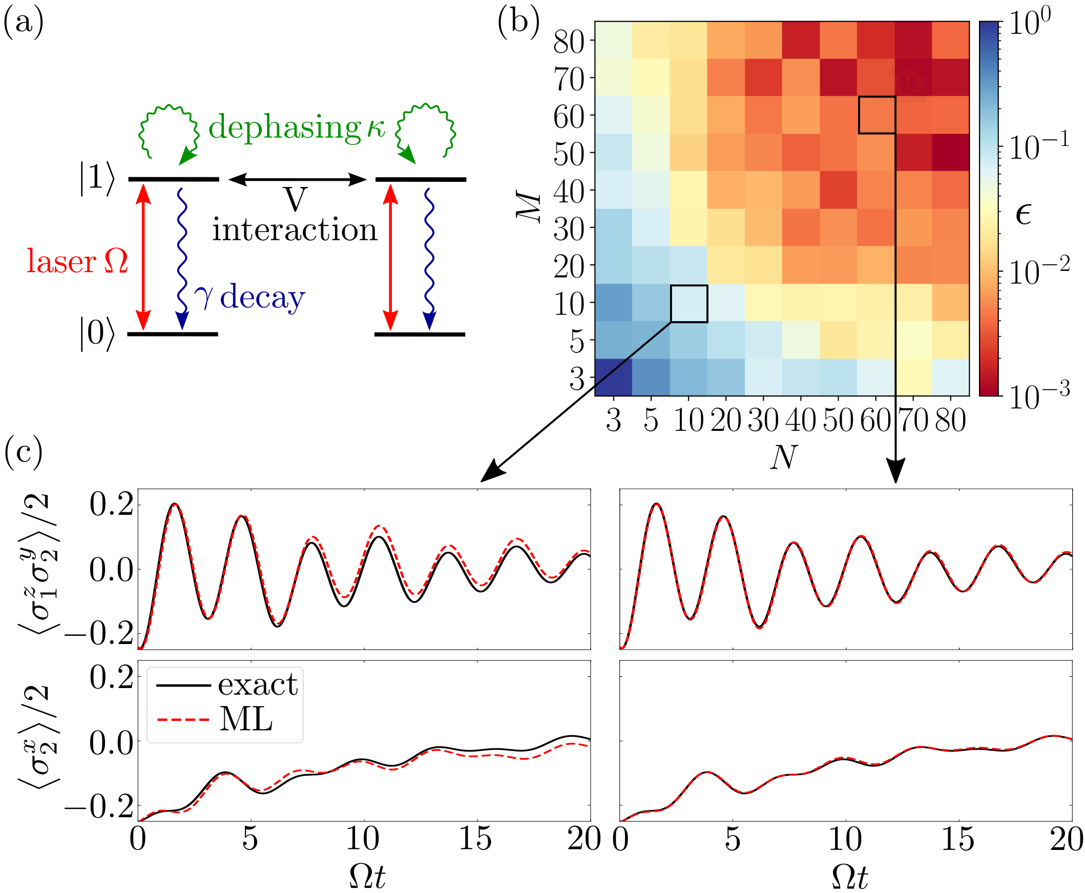
Figure 2: Benchmark. (a) Open system used to benchmark the ML algorithm, described in terms of a Hamiltonian and jump operators [cf. Eq. (10)]. The Hamiltonian consists of a driving ($\Omega$) and an interaction ($V$). Jump operators describe decay (with rate $\gamma$) and dephasing (with rate $\kappa$). (b) The error $\epsilon(N,M)$ as in Eq. (9) plotted for different values of $N$ and $M$. The error is averaged over $r=10$ out-of-sample trajectories with a doubled time-window $[0,2\Omega T]$ (see main text for details). (c) Dynamical curves for two selected observables and different combinations of $N$ and $M$. From the plot one can appreciate how the predicted dynamics is already quite reliable for smaller values of $N$ and $M$. The parameters are $V=0.5\Omega$, $\gamma=0.01\Omega$ and $\kappa=0.05\Omega$.

Before training the algorithm on data for the many-body model in Eq. (1), we benchmark its ability to learn a Lindblad generator within a well-controlled setting. To this end we consider a two-spin Lindblad generator, which in its diagonal form, is specified by the following Hamiltonian and jump operators [cf. Fig. 2(a)]

$$H =\frac{\Omega}{2}(\sigma_{1}^{x}+\sigma_{2}^{x})+Vn_{1}n_{2}\,,$$

$$J_{1} =\sqrt{\gamma}\sigma_{1}^{-}\,,\qquad J_{2}=\sqrt{\gamma}\sigma_{2}^{-}\,,$$ (10)

$$J_{3} =\sqrt{\kappa}n_{1}\,,\qquad J_{4}=\sqrt{\kappa}n_{2}\,.$$

The jump operators effectively describe the effects of the environment on the subsystem. In particular, $J_{1},J_{2}$ encode decay from $\ket{1}$ to $\ket{0}$ while $J_{3},J_{4}$ encode dephasing. The data generation procedure follows the protocol described above, with two exceptions: the initial conditions are given by a random density matrix $\rho_{\mathrm{rand}}$, and the data for testing have a doubled time-window $[0,2\Omega T]$. In this way, we can also test the ability of the algorithm to extrapolate to unseen times. Since the network is, in principle, able to perfectly learn a Markovian Lindblad generator, we expect the extrapolation to be accurate. The results are reported in Fig. 2 (b-c). The color map [panel (b)] shows the error, $\epsilon(N,M)$, averaged over $r=10$ test trajectories, for 100 different combinations of $N$ and $M$. First, we observe the overall trend of the error to decrease as $N\times M$ increases. However, the plot is not symmetric with respect to the line $M=N$. In fact, for higher values of $M$ (and fixed $N\times M$), the ML algorithm has a more stable training, and hence a better performance. This is due to the fact that the choice of the $M$ time-points is random, and a small value of $M$ has a high probability of yielding data which is not representative of the dynamics. On the other hand, higher values of $M$ yields more representative data of the trajectory, despite relatively small values of $N$. For high values of $N$ and $M$, as expected, the error becomes small. The ML algorithm can thus successfully learn a Lindbladian, with a precision that approximately depends on the product $N\times M$.

Many-body setting.—

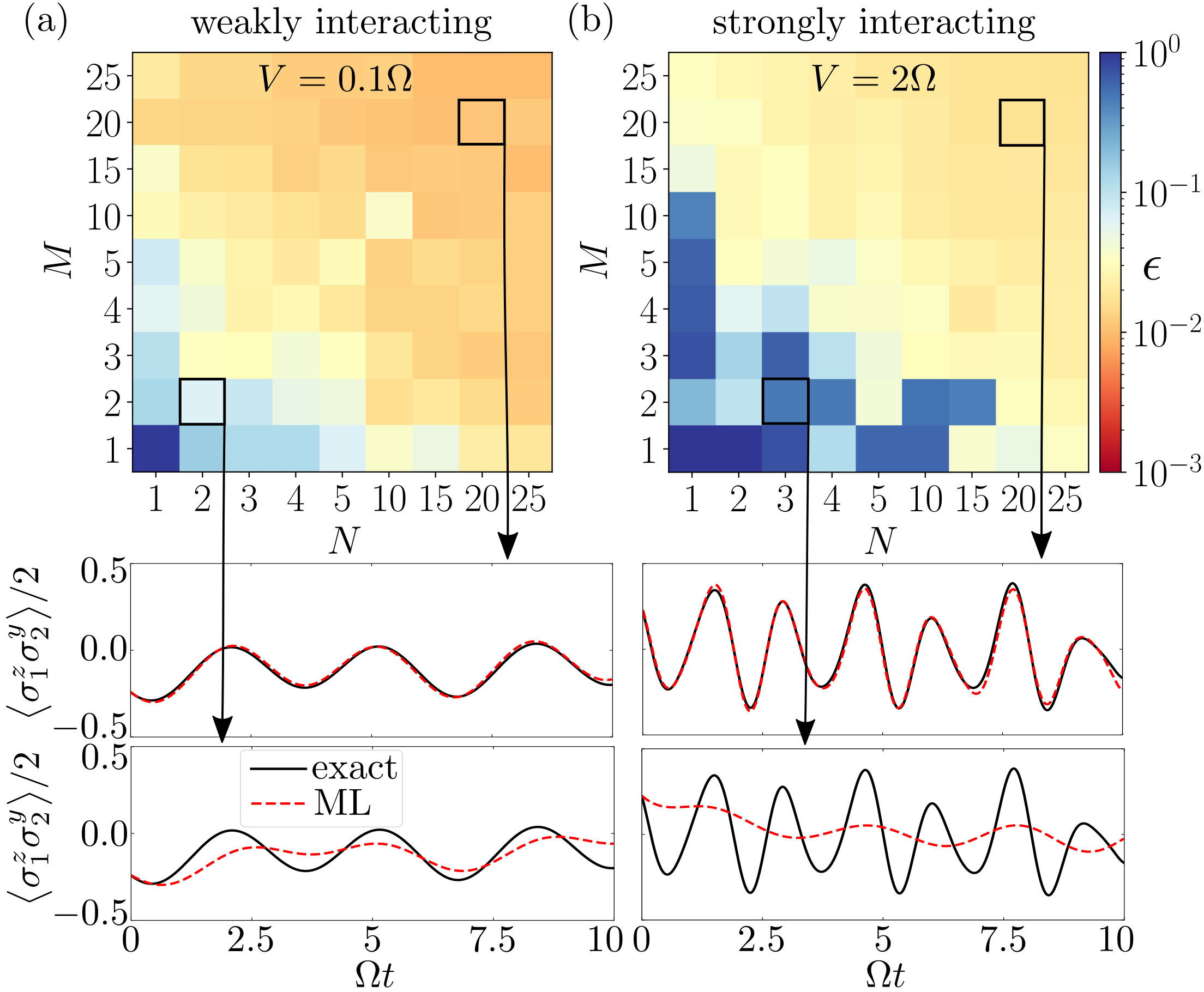
Figure 3: Learning the subsystem dynamics. Error $\epsilon(N,M)$ as in Eq. (9) for different values of $N$ and $M$, for two different combinations of the parameters. The error is calculated over $r=10$ trajectories with $t\in[0,\Omega T]$. (a) Data for the case $V=0.1\Omega$. Here, the dynamics is slow and the ML algorithm learns an effective $\mathcal{L}$ already for small values of $N$ and $M$. (b) Data for $V=2\Omega$. In this case, two different regimes can be distinguished neatly: either the model does not learn the dynamics (blue squares) or it learns it (yellow squares). In both cases, the errors are due to the non-Markovianity assumed for the learned model. The plots beneath the color maps reports the time evolution of an observable for the two different models and different sets of $(N,M)$.

Having established the capability of the ML algorithm to exactly learn Lindblad generators from experimental data, we now address the many-body scenario described by Eq. (1). In this case, the reduced dynamics of the state $\rho_{\rm S}(t)$ can feature non-Markovian effects. The ML algorithm will thus, by construction, learn the “optimal” Markovian description of the system. Whether this description will accurately describe the subsystem or not depends on the relevance of non-Markovian effects.

In Fig. 3(a), we show results for weak interactions $V=0.1\Omega$. In this case, the ML algorithm learns a dynamical generator which faithfully reproduces the time evolution of the coherence vector. This suggests that the subsystem dynamics is, in this weak-coupling regime, essentially Markovian. Notably, the Lindblad generator can inferred even when $N$ and $M$ are small. As already observed during the benchmarking, the training procedure is less stable for the models in the bottom-right corner of Fig. 3(a), compared to the top left, confirming that larger $M$ values are better than larger $N$ values at fixed $N\times M$.

In Fig. 3(b) we show instead results for strong interactions, $V=2\Omega$. Quite surprisingly, also in this case, the ML algorithm learns an effective Lindbladian which reproduces very well the subsystem dynamics. Also in this case, the latter has a Markovian character. A possible explanation for this is that strong interactions lead to a faster decay of time correlations in the environment, which thus renders the subsystem dynamics Markovian. Due to the faster oscillations in this regime, more sampling points in time are needed than the weakly interacting case, Fig. 3(a), for a same accuracy. In both cases, for small $N\times M$, while the model cannot recover the exact dynamics, it nonetheless provides an average over the fast oscillations [cf. Figs. 3(a)-3(b)]. The data for the whole coherence vector are reported in the supplemental material [52], where we also show additional results on the case $V=0.5\Omega$. In the latter case, the error is higher, due to non-Markovian effects which appear to be non-negligible [56] in this intermediate regime.

Conclusions.— We have presented a simple ML algorithm able to learn a physically consistent and interpretable dynamical generator starting from (synthetic) experimental data. We have shown that it can yield faithful results for both weak and strong interactions. A wider range of systems could be included by relaxing the assumed Markovianity of the learned generator, namely by allowing it to be time-dependent $\mathcal{L}(t)$. Some approaches already exist (see, e.g., Refs. [39, 36]), but they require an enormous amount of data and lack physical interpretability.

Our ML method is interpretable, hence it can be used to “read out” the underlying dynamical processes (see Supplemental Material [52]). In fact, the learned matrix $\mathbf{L}$ gives direct access to the parameters $\theta^{H}_{i},\theta^{X}_{ij},\theta^{Y}_{ij}$, which represent the Hamiltonian and the jump operators of the subsystem S. In the future, it would be interesting to understand whether feeding the ML algorithm with a sampling of the full coherence vector is necessary or whether a bona fide dynamics can still be learned when leaving out information about certain observables.

Acknowledgments.— We acknowledge financial support from the Deutsche Forschungsgemeinschaft (DFG, German Research Foundation) under Germany’s Excellence Strategy—EXC-Number 2064/1-Project Number 390727645, under Project No. 449905436 and through the Research Unit FOR 5413/1, Grant No. 465199066. This project has also received funding from the European Union’s Horizon Europe research and innovation program under Grant Agreement No. 101046968 (BRISQ). FC is indebted to the Baden-Württemberg Stiftung for the financial support of this research project by the Eliteprogramme for Postdocs.

SUPPLEMENTAL MATERIAL

Inferring interpretable dynamical generators of local quantum observables from projective measurements through machine learning

I. Matrix representation of $\mathbf{L}$

We here report a brief derivation of the explicit matrix elements appearing in eq. (5). The stating point is the coherence vector $v_{i}=\Tr(F_{i}\rho_{S})$. The time derivative is simply given by

$$\frac{d}{dt}v_{i}(t)=\Tr\bigg(F_{i}\frac{d}{dt}\rho_{S}(t)\bigg{missing})=\Tr(F_{i}\mathcal{L}[\rho_{S}(t)])=\Tr(\mathcal{L}^{*}[F_{i}]\rho_{S}(t))$$ (S1)

where in the second equality we used eq. (2). In the last equality $\mathcal{L}^{*}$ is the dual map of $\mathcal{L}$, i.e. the one evolving observables instead of states. By expanding the dual map $\mathcal{L}^{*}[F_{i}]=\sum_{j=1}^{d^{2}}\Tr(\mathcal{L}^{*}[F_{i}]F_{j})F_{j}$, and substituting into eq. (S1), one obtains

$$\frac{d}{dt}v_{i}(t)=\sum_{j=1}^{d^{2}}\Tr(\mathcal{L}^{*}[F_{i}]F_{j})\Tr(F_{j}\rho_{S})=[\mathbf{Lv}(t)]_{i}\,,$$ (S2)

where we defined the matrix $\mathbf{L}$ as $\mathbf{L}_{ij}\equiv\Tr(\mathcal{L}^{*}[F_{i}]F_{j})$. By exploiting the cyclic property of the trace, one can explicitly calculate $\mathcal{L}^{*}[F_{i}]$ starting from the known action of $\mathcal{L}[\rho]$. Explicitly we obtain

$$\Tr(\mathcal{L}^{*}[F_{k}]F_{l})=\Tr\bigg(i[H,F_{k}]F_{l}+\frac{1}{2}\sum_{i,j=2}^{d^{2}}c_{ij}(F^{\dagger}_{j}[F_{k},F_{i}]F_{l}+[F^{\dagger}_{j},F_{k}]F_{i}F_{l})\bigg{missing})\,.$$ (S3)

Comparing this result to eq. (5) we obtain

$$\mathbf{H}_{kl}=i\Tr([H,F_{k}]F_{l})\,,\qquad\mathbf{D}_{kl}=\frac{1}{2}\sum_{i,j=2}^{d^{2}}c_{ij}\Tr(F^{\dagger}_{j}[F_{k},F_{i}]F_{l}+[F^{\dagger}_{j},F_{k}]F_{i}F_{l})\,.$$ (S4)

To simplify this expressions we use the structure constants $d_{ijk}$ and $f_{ijk}$, defined from the commutation and anticommutaton relations as

$$d_{ijk}=\frac{1}{4}\Tr(\{F_{i},F_{j}\}F_{k})\,,$$ (S5)

$$f_{ijk}=-\frac{i}{4}\Tr([F_{i},F_{j}]F_{k})\,.$$ (S6)

By substituting those definitions into eq. (S4), we obtain the following expressions for the matrix elements of $\mathbf{H}$

$$\mathbf{H}_{ij} =-4\sum_{k=2}^{d^{2}}f_{ijk}\theta^{H}_{k}\,,\quad i,j\in\{2,...,d^{2}\}$$ (S7)

$$\mathbf{H}_{i1} =\mathbf{H}_{1i}=0\,,\quad i\in\{1,...,d^{2}\}$$

where $\theta^{H}_{k}$ provides the expansion of the Hamiltonian over the basis $F_{i}$, namely $H=\sum_{i=2}^{i=d^{2}}F_{i}\theta^{H}_{i}$. The matrix elements of $\mathbf{D}$ reads

$$\mathbf{D}_{mn} =-8\sum_{i,j,k=2}^{d^{2}}f_{mik}(f_{njk}\real(c)_{ij}+d_{njk}\imaginary(c)_{ij})\,, m,n\in\{2,...,d^{2}\}$$ (S8)

$$\mathbf{D}_{m1} =2\sum_{i,j=2}^{d^{2}}f_{imj}\imaginary(c)_{ij}\,,\quad\mathbf{D}_{1m}=0\,, m\in\{1,...,d^{2}\}$$

where $c_{ij}$ is the so-called Kossakowski matrix, which we parametrized as $c=Z^{\dagger}Z$ with $Z=\theta^{X}+i\theta^{Y}$ and $\theta^{X}$,$\theta^{Y}$ real matrices.

Equations (S7) and (S8) are the matrix representation of the Lindblad operator $\mathcal{L}$ in terms of the vector $\omega_{i}$ and the Kossakowski matrix $c_{ij}$.

II. Further results

In the main text, we investigate the behavior of the ML framework applied to spin chains having $V=0.1\Omega,2\Omega$. Here we report the case of a spin chain having $V=0.5\Omega$. The results are shownin Figure S1. The graph exhibits a similar behavior to the cases analyzed in the main text. However, there is a notable distinction: the model saturates at a higher error. This discrepancy arises from the stronger coupling between the system and the bath, rendering non-Markovian effects non-negligible.

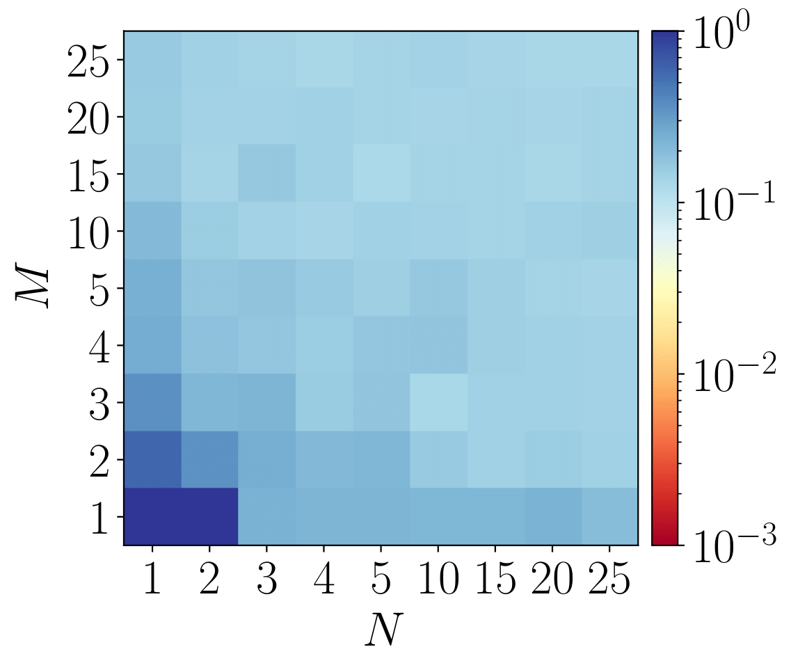
Figure S1: ML algorithm’s performance on open system dynamics. The figure reports the error $\epsilon(N,M)$ as in (9) plotted for different values of $N$ and $M$, and for the $V=0.5\Omega$ spin chain.

III. Additional plots and physical “read out”

For completeness, we report here the plots of all $15$ non-trivial components of the coherence vector $v_{i}$. The plots represent the exact time evolution (black solid line) and the dynamics predicted by the ML algorithm (red dashed line).

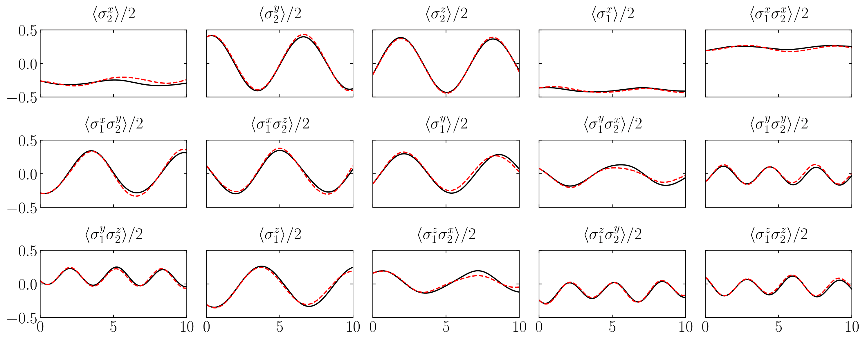
Figure S2: Full plot of the ML algorithm’s performance. In figure the $15$ non-trivial components of the coherence vector $v_{i}$. The data refers to a spin chain with $V=0.1\Omega$, and $N=20,M=20$. The plots represent the exact time evolution (black solid line) and the dynamics predicted by the ML algorithm (red dashed line). In this case, the overall dynamics is roughly captured.

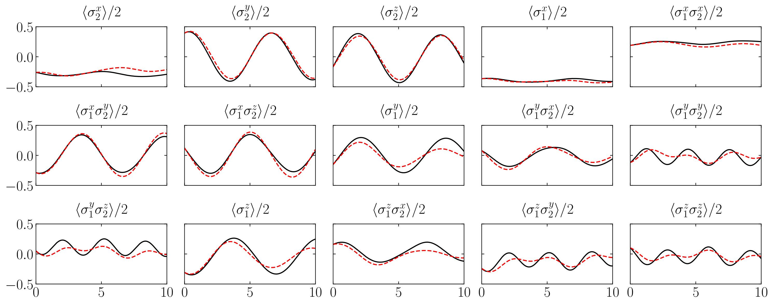
Figure S3: Full plot of the ML algorithm’s performance. In figure the $15$ non-trivial components of the coherence vector $v_{i}$. The data refers to a spin chain with the same parameters as in Fig. S2, but $N=2,M=2$. The plots represent the exact time evolution (black solid line) and the dynamics predicted by the ML algorithm (red dashed line). In this case, the overall dynamics is well captured.

In Figure S2 and S3 we report the performance of the model trained on data that refers to a spin chain with $V=0.1\Omega$. In Fig. S2 the synthetic experimental data is generated with $N=20,M=20$. In this case, the ML prediction is almost perfectly overlapped on the exact line, indicating the correctness of the learned Lindbladian. In Fig. S3 the synthetic experimental data is generated with $N=2,M=2$. In this case, the dynamics is roughly captured, made exception for some observables e.g., $\sigma^{y}_{1}\sigma^{y}_{2},\sigma^{y}_{1}\sigma^{z}_{2},\sigma^{z}_{1}\sigma^{y}_{2}\text{ and }\sigma^{z}_{1}\sigma^{z}_{2},$.

In addition to the complete plots, we here report the learned expressions for the Hamiltonian and jump operators. In this case, we take into consideration the model trained over $N=20$ and $M=20$. For the Hamiltonian, we round up to two decimal places to improve readability; it reads

$$H=0.5(\sigma^{x}_{1}+\sigma^{x}_{2})+0.055(\sigma^{z}_{1}+\sigma^{z}_{2})+0.025\,\sigma^{z}_{1}\sigma^{z}_{2}-0.03(\sigma^{y}_{1}+\sigma^{y}_{2})+0.005(-\sigma^{z}_{1}\sigma^{x}_{2}-\sigma^{y}_{1}\sigma^{x}_{2}+\sigma^{z}_{1}\sigma^{y}_{2}-\sigma^{x}_{1}\sigma^{z}_{2}+\sigma^{x}_{1}\sigma^{y}_{2})\,.$$

Regarding dissipation part, there is only one non-zero eigenvalue (rounded to three decimal places) of the Kossakowski matrix $\gamma=0.013$. Regarding the jump operator, rounded up to two decimal places, it reads

$$J= 0.245\,\sigma^{x}_{1}\sigma^{z}_{2}+(0.19-0.1i)\,\sigma_{2}^{y}+(-0.16+0.07i)\,\sigma^{x}_{1}\sigma^{y}_{2}+(0.055+0.145i)\,\sigma_{1}^{y}\sigma_{2}^{y}+(0.095-0.075i)\,\sigma_{1}^{y}+$$

$$+(-0.09-0.08i)\,\sigma_{1}^{y}\sigma_{2}^{x}-(0.05+0.105i)\,\sigma_{1}^{x}+(0.09-0.065i)\,\sigma_{1}^{x}\sigma_{2}^{x}+(0.03-0.1i)\,\sigma^{z}_{1}\sigma^{x}_{2}+(-0.09+0.02i)\,\sigma_{1}^{z}+$$

$$+(0.005+0.08i)\,\sigma_{1}^{z}\sigma_{2}^{x}+(-0.03+0.06i)\,\sigma_{1}^{z}\sigma_{2}^{z}+(0.02+0.035i)\,\sigma_{1}^{y}\sigma_{2}^{z}+0.005\,\sigma_{2}^{z}$$

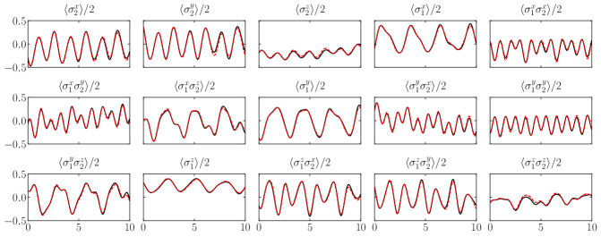
Figure S4: Full plot of the ML algorithm’s performance. In figure the $15$ non-trivial components of the coherence vector $v_{i}$. The data refers to a spin chain with $V=2\Omega$, and $N=20,M=20$. The plots represent the exact time evolution (black solid line) and the dynamics predicted by the ML algorithm (red dashed line). In this case, the overall dynamics is porly captured.

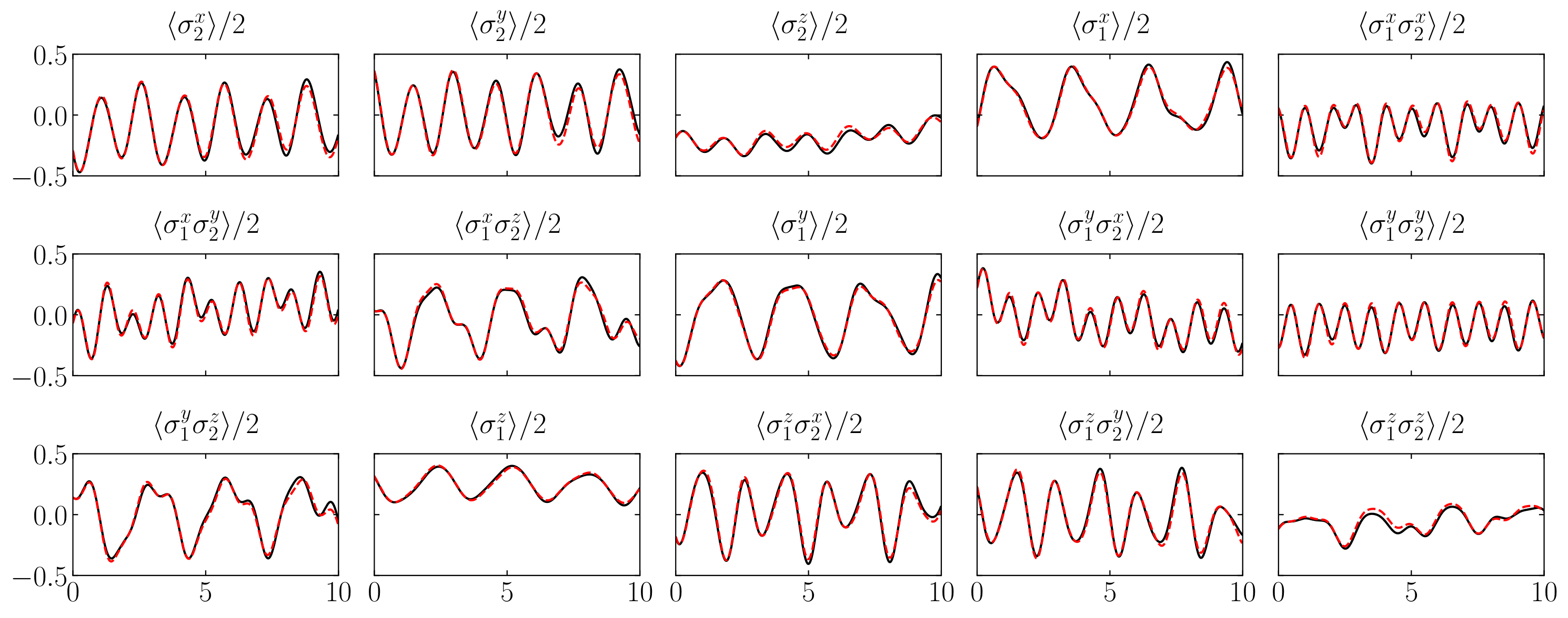
Figure S5: Full plot of the ML algorithm’s performance. In figure the $15$ non-trivial components of the coherence vector $v_{i}$. The data refers to a spin chain with the same parameters as in Fig. S4, but $N=3,M=2$. The plots represent the exact time evolution (black solid line) and the dynamics predicted by the ML algorithm (red dashed line). In this case, the overall dynamics is well captured.

In Figure S4 and S5 we report the performance of the model trained on data that refers to a spin chain with $V=2\Omega$. In Fig. S4 the synthetic experimental data is generated with $N=20,M=20$. In this case, the ML prediction is almost perfectly overlapped on the exact line, indicating the correctness of the learned Lindbladian. In Fig. S3 the synthetic experimental data is generated with $N=3,M=2$. In this case, the dynamics is poorly captured.

References

- Chertkov and Clark [2018] E. Chertkov and B. K. Clark, Computational inverse method for constructing spaces of quantum models from wave functions, Phys. Rev. X 8, 031029 (2018).
- Zache et al. [2020] T. V. Zache, T. Schweigler, S. Erne, J. Schmiedmayer, and J. Berges, Extracting the field theory description of a quantum many-body system from experimental data, Phys. Rev. X 10, 011020 (2020).
- Merger et al. [2023] C. Merger, A. René, K. Fischer, P. Bouss, S. Nestler, D. Dahmen, C. Honerkamp, and M. Helias, Learning interacting theories from data (2023), arXiv:2304.00599 .
- Liu et al. [2011] B.-H. Liu, L. Li, Y.-F. Huang, C.-F. Li, G.-C. Guo, E.-M. Laine, H.-P. Breuer, and J. Piilo, Experimental control of the transition from Markovian to non-Markovian dynamics of open quantum systems, Nat. Phys. 7, 931 (2011).
- Navarrete-Benlloch et al. [2011] C. Navarrete-Benlloch, I. de Vega, D. Porras, and J. I. Cirac, Simulating quantum-optical phenomena with cold atoms in optical lattices, New J. Phys. 13, 023024 (2011).
- Ma et al. [2012] J. Ma, Z. Sun, X. Wang, and F. Nori, Entanglement dynamics of two qubits in a common bath, Phys. Rev. A 85, 062323 (2012).
- Everest et al. [2017] B. Everest, I. Lesanovsky, J. P. Garrahan, and E. Levi, Role of interactions in a dissipative many-body localized system, Phys. Rev. B 95, 024310 (2017).
- Hoeppe et al. [2012] U. Hoeppe, C. Wolff, J. Küchenmeister, J. Niegemann, M. Drescher, H. Benner, and K. Busch, Direct observation of non-Markovian radiation dynamics in 3D bulk photonic crystals, Phys. Rev. Lett. 108, 043603 (2012).
- Georgescu et al. [2014] I. M. Georgescu, S. Ashhab, and F. Nori, Quantum simulation, Rev. Mod. Phys. 86, 153 (2014).
- Weimer et al. [2010] H. Weimer, M. Müller, I. Lesanovsky, P. Zoller, and H. P. Büchler, A Rydberg quantum simulator, Nat. Phys. 6, 382 (2010).
- Friedenauer et al. [2008] A. Friedenauer, H. Schmitz, J. T. Glueckert, D. Porras, and T. Schätz, Simulating a quantum magnet with trapped ions, Nat. Phys. 4, 757 (2008).
- Cirac and Zoller [2012] J. I. Cirac and P. Zoller, Goals and opportunities in quantum simulation, Nat. Phys. 8, 264 (2012).
- Blatt and Roos [2012] R. Blatt and C. F. Roos, Quantum simulations with trapped ions, Nat. Phys. 8, 277 (2012).
- Babbush et al. [2023] R. Babbush, W. J. Huggins, D. W. Berry, S. F. Ung, A. Zhao, D. R. Reichman, H. Neven, A. D. Baczewski, and J. Lee, Quantum simulation of exact electron dynamics can be more efficient than classical mean-field methods (2023), arXiv:2301.01203 .
- Jin et al. [2023] S. Jin, N. Liu, X. Li, and Y. Yu, Quantum simulation for quantum dynamics with artificial boundary conditions (2023), arXiv:2304.00667 .
- Zhang et al. [2023] X. Zhang, E. Kim, D. K. Mark, S. Choi, and O. Painter, A superconducting quantum simulator based on a photonic-bandgap metamaterial, Science 379, 278 (2023).
- Schäfer et al. [2020] F. Schäfer, T. Fukuhara, S. Sugawa, Y. Takasu, and Y. Takahashi, Tools for quantum simulation with ultracold atoms in optical lattices, Nat. Rev. Phys. 2, 411 (2020).
- Carrasco et al. [2021] J. Carrasco, A. Elben, C. Kokail, B. Kraus, and P. Zoller, Theoretical and experimental perspectives of quantum verification, PRX Quantum 2, 010102 (2021).
- Hauke et al. [2012] P. Hauke, F. M. Cucchietti, L. Tagliacozzo, I. Deutsch, and M. Lewenstein, Can one trust quantum simulators?, Rep. Prog. Phys. 75, 082401 (2012).
- Altman et al. [2021] E. Altman, K. R. Brown, G. Carleo, L. D. Carr, E. Demler, C. Chin, B. DeMarco, S. E. Economou, M. A. Eriksson, K.-M. C. Fu, M. Greiner, K. R. Hazzard, R. G. Hulet, A. J. Kollár, B. L. Lev, M. D. Lukin, R. Ma, X. Mi, S. Misra, C. Monroe, K. Murch, Z. Nazario, K.-K. Ni, A. C. Potter, P. Roushan, M. Saffman, M. Schleier-Smith, I. Siddiqi, R. Simmonds, M. Singh, I. Spielman, K. Temme, D. S. Weiss, J. Vučković, V. Vuletić, J. Ye, and M. Zwierlein, Quantum simulators: Architectures and opportunities, PRX Quantum 2, 017003 (2021).
- Morgado and Whitlock [2021] M. Morgado and S. Whitlock, Quantum simulation and computing with Rydberg-interacting qubits, AVS Quantum Sci. 3, 10.1116/5.0036562 (2021), 023501.
- Gebhart et al. [2023] V. Gebhart, R. Santagati, A. A. Gentile, E. M. Gauger, D. Craig, N. Ares, L. Banchi, F. Marquardt, L. Pezzè, and C. Bonato, Learning quantum systems, Nat. Rev. Phys. 5, 141 (2023).
- Braccia et al. [2022] P. Braccia, L. Banchi, and F. Caruso, Quantum noise sensing by generating fake noise, Phys. Rev. Appl. 17, 024002 (2022).
- Han et al. [2021] C.-D. Han, B. Glaz, M. Haile, and Y.-C. Lai, Tomography of time-dependent quantum Hamiltonians with machine learning, Phys. Rev. A 104, 062404 (2021).
- Mohseni et al. [2022] N. Mohseni, T. Fösel, L. Guo, C. Navarrete-Benlloch, and F. Marquardt, Deep learning of quantum many-body dynamics via random driving, Quantum 6, 714 (2022).
- Genois et al. [2021] É. Genois, J. A. Gross, A. Di Paolo, N. J. Stevenson, G. Koolstra, A. Hashim, I. Siddiqi, and A. Blais, Quantum-tailored machine-learning characterization of a superconducting qubit, PRX Quantum 2, 040355 (2021).
- Wilde et al. [2022] F. Wilde, A. Kshetrimayum, I. Roth, D. Hangleiter, R. Sweke, and J. Eisert, Scalably learning quantum many-body Hamiltonians from dynamical data (2022), arXiv:2209.14328 .
- Bairey et al. [2019] E. Bairey, I. Arad, and N. H. Lindner, Learning a local Hamiltonian from local measurements, Phys. Rev. Lett. 122, 020504 (2019).
- Di Franco et al. [2009] C. Di Franco, M. Paternostro, and M. Kim, Hamiltonian tomography in an access-limited setting without state initialization, Phys. Rev. Lett. 102, 187203 (2009).
- Cole et al. [2005] J. H. Cole, S. G. Schirmer, A. D. Greentree, C. J. Wellard, D. K. Oi, and L. C. Hollenberg, Identifying an experimental two-state Hamiltonian to arbitrary accuracy, Phys. Rev. A 71, 062312 (2005).
- Devitt et al. [2006] S. J. Devitt, J. H. Cole, and L. C. Hollenberg, Scheme for direct measurement of a general two-qubit Hamiltonian, Phys. Rev. A 73, 052317 (2006).
- Wang et al. [2017] J. Wang, S. Paesani, R. Santagati, S. Knauer, A. A. Gentile, N. Wiebe, M. Petruzzella, J. L. O’Brien, J. G. Rarity, A. Laing, et al., Experimental quantum Hamiltonian learning, Nat. Phys. 13, 551 (2017).
- Gentile et al. [2021] A. A. Gentile, B. Flynn, S. Knauer, N. Wiebe, S. Paesani, C. E. Granade, J. G. Rarity, R. Santagati, and A. Laing, Learning models of quantum systems from experiments, Nat. Phys. 17, 837 (2021).
- Nakajima [1958] S. Nakajima, On quantum theory of transport phenomena: steady diffusion, Prog. Theor. Phys. 20, 948 (1958).
- Zwanzig [1960] R. Zwanzig, Ensemble method in the theory of irreversibility, J. Chem. Phys. 33, 1338 (1960).
- Cerrillo and Cao [2014] J. Cerrillo and J. Cao, Non-Markovian dynamical maps: numerical processing of open quantum trajectories, Phys. Rev. Lett. 112, 110401 (2014).
- Gelzinis et al. [2017] A. Gelzinis, E. Rybakovas, and L. Valkunas, Applicability of transfer tensor method for open quantum system dynamics, J. Chem. Phys. 147, 234108 (2017).
- Pollock and Modi [2018] F. A. Pollock and K. Modi, Tomographically reconstructed master equations for any open quantum dynamics, Quantum 2, 76 (2018).
- Banchi et al. [2018] L. Banchi, E. Grant, A. Rocchetto, and S. Severini, Modelling non-Markovian quantum processes with recurrent neural networks, New J. Phys. 20, 123030 (2018).
- Link et al. [2023] M. Link, K. Gao, A. Kell, M. Breyer, D. Eberz, B. Rauf, and M. Köhl, Machine learning the phase diagram of a strongly interacting fermi gas, Phys. Rev. Lett. 130, 203401 (2023).
- Wu et al. [2021] X. Wu, X. Liang, Y. Tian, F. Yang, C. Chen, Y.-C. Liu, M. K. Tey, and L. You, A concise review of Rydberg atom based quantum computation and quantum simulation*, Chin. Phys. B 30, 020305 (2021).
- Saffman et al. [2010] M. Saffman, T. G. Walker, and K. Mølmer, Quantum information with Rydberg atoms, Rev. Mod. Phys. 82, 2313 (2010).
- Mazza et al. [2021] P. P. Mazza, D. Zietlow, F. Carollo, S. Andergassen, G. Martius, and I. Lesanovsky, Machine learning time-local generators of open quantum dynamics, Phys. Rev. Res. 3, 023084 (2021).
- Carnazza et al. [2022] F. Carnazza, F. Carollo, D. Zietlow, S. Andergassen, G. Martius, and I. Lesanovsky, Inferring Markovian quantum master equations of few-body observables in interacting spin chains, New J. Phys. 24, 073033 (2022).
- Breuer and Petruccione [2002] H. P. Breuer and F. Petruccione, The theory of open quantum systems (Oxford University Press, Great Clarendon Street, 2002).
- Gorini et al. [1976] V. Gorini, A. Kossakowski, and E. C. G. Sudarshan, Completely positive dynamical semigroups of N-level systems, J. Math. Phys. 17, 821 (1976).
- Lindblad [1976] G. Lindblad, On the generators of quantum dynamical semigroups, Commun. Math. Phys. 48, 119 (1976).
- Vidal [2004] G. Vidal, Efficient simulation of one-dimensional quantum many-body systems, Phys. Rev. Lett. 93, 040502 (2004).
- Zwolak and Vidal [2004] M. Zwolak and G. Vidal, Mixed-state dynamics in one-dimensional quantum lattice systems: a time-dependent superoperator renormalization algorithm, Phys. Rev. Lett. 93, 207205 (2004).
- Gray [2018] J. Gray, quimb: a python library for quantum information and many-body calculations, Journal of Open Source Software 3, 819 (2018).
- Byrd and Khaneja [2003] M. S. Byrd and N. Khaneja, Characterization of the positivity of the density matrix in terms of the coherence vector representation, Phys. Rev. A 68, 062322 (2003).
- [52] See Supplemental Material for details.
- Imambi et al. [2021] S. Imambi, K. B. Prakash, and G. Kanagachidambaresan, Pytorch, Programming with TensorFlow: Solution for Edge Computing Applications , 87 (2021).
- Kingma and Ba [2014] D. P. Kingma and J. Ba, Adam: A method for stochastic optimization (2014), arXiv:1412.6980 .
- Note [1] The code for the generation of the artificial data and the training of the ML algorithm is made available at https://github.com/giovannicemin/lindblad_dynamics_approximator.
- Roos et al. [2020] J. Roos, J. I. Cirac, and M. C. Bañuls, Markovianity of an emitter coupled to a structured spin-chain bath, Phys. Rev. A 101, 042114 (2020).