DANSE: Data-driven Non-linear State Estimation of Model-free Process in Unsupervised Learning Setup

Abstract

We address the tasks of Bayesian state estimation and forecasting for a model-free process in an unsupervised learning setup. In the article, we propose DANSE – a Data-driven Nonlinear State Estimation method. DANSE provides a closed-form posterior of the state of the model-free process, given linear measurements of the state. In addition, it provides a closed-form posterior for forecasting. A data-driven recurrent neural network (RNN) is used in DANSE to provide the parameters of a prior of the state. The prior depends on the past measurements as input, and then we find the closed-form posterior of the state using the current measurement as input. The data-driven RNN captures the underlying non-linear dynamics of the model-free process. The training of DANSE, mainly learning the parameters of the RNN, is executed using an unsupervised learning approach. In unsupervised learning, we have access to a training dataset comprising only a set of measurement data trajectories, but we do not have any access to the state trajectories. Therefore, DANSE does not have access to state information in the training data and can not use supervised learning. Using simulated linear and non-linear process models (Lorenz attractor and Chen attractor), we evaluate the unsupervised learning-based DANSE. We show that the proposed DANSE, without knowledge of the process model and without supervised learning, provides a competitive performance against model-driven methods, such as the Kalman filter (KF), extended KF (EKF), unscented KF (UKF), and a recently proposed hybrid method called KalmanNet.

I Introduction

Context: Estimating the state $\mathbf{x}_{t}$ of a complex dynamical system/process from noisy measurements/observations $\mathbf{y}_{t}$, maintaining causality, is a fundamental problem in the field of signal processing, control, and machine learning. Here, $t$ denotes a discrete time index. In a Bayesian setup, for state estimation, we wish to find a closed-form posterior of the state given the current and past measurements, which means $p(\mathbf{x}_{t}|\mathbf{y}_{t},\mathbf{y}_{t-1},\ldots,\mathbf{y}_{1})$.

For the state estimation problem, traditional Bayesian methods assume that the model of state dynamics (also called process model/state model) is known. Examples of such model-driven methods are the Kalman filter (KF) and its extensions such as the extended KF (EKF), the unscented KF (UKF), and sampling-based methods such as particle filters [1, 2, 3, 4, 5]. We assume that the model in a model-driven method (also referred to as model-based) is formed using the physics of the process and/or some a-priori knowledge, and there is no need for learning (or training). On the other hand, modern data-driven methods use deep neural networks (DNNs), mainly recurrent neural networks (RNNs), to map $\mathbf{y}_{t}$ to $\mathbf{x}_{t}$ directly, without knowing the process model. The data-driven methods can handle complex model-free processes using a supervised learning-based training approach. At the training phase, supervised learning requires to access state $\mathbf{x}_{t}$ to have a labelled dataset in a pairwise formation $(\mathbf{y}_{t},\mathbf{x}_{t})$. The labelled dataset is used to train the data-driven RNNs.

Motivation: There are many scenarios where the physics of the process is unknown/limited, and the state $\mathbf{x}_{t}$ is not accessible due to practical reasons. Inaccessible state $\mathbf{x}_{t}$ does not allow to have a labelled dataset. Therefore, we can not engineer model-driven methods and supervised learning-based data-driven methods. The main question is: Can we develop a Bayesian estimator of $\mathbf{x}_{t}$ for a complex model-free process without any access to $\mathbf{x}_{t}$, but using an unsupervised learning approach based on a training dataset comprised of measurements $\mathbf{y}_{t}$? The purpose of the article is to develop DANSE (Data-driven Nonlinear State Estimation) to answer the above question. This is based on our recent contribution [6].

Potential applications: DANSE has potential applications when there are enough measurements for unsupervised learning, but it is difficult to access the state for supervised learning and/or design a good tractable process model. For example, we can explore the use of DANSE for internal state estimation of a medical patient from physiological time-series data. Another example is positioning and navigation of autonomous systems in hazardous, underwater, off-road conditions where GPS (global positioning system) signal is not available to know the state [7] and create labelled data for supervised learning.

Aspects of DANSE:

1. It is for a model-free process where the state dynamics are expected to be non-linear and complex.

2. Unsupervised learning of DANSE is realized using a standard maximum-likelihood principle.

3. For linear measurements, it provides closed-form posterior $p(\mathbf{x}_{t}|\mathbf{y}_{t},\mathbf{y}_{t-1},\ldots,\mathbf{y}_{1})$ in terms of RNN parameters.

4. It is a causal system, and suitable for forecasting problems. Also can be modified for use without causality.

Attribute	Methods/Approaches
	Model-based	Data-driven	Hybrid	DANSE
	e.g. KF, EKF, UKF, etc.	e.g. DVAE, RNNs, etc.	e.g. KalmanNet
Domain knowledge
Process state dynamics (SSM)	✓	✗	✓	✗
Process noise statistics	✓	✗	✗	✗
Measurement system	✓	✗	✓	✓
Measurement noise statistics	✓	✗	✗	✓
Learning and Inference
Supervised learning	—	✓ / ✗	✓ / ✗	✗
Closed-form posterior	✓	✗	✓	✓

TABLE I: A visualization of attributes for different methods/approaches: model-driven, data-driven, hybrid, and DANSE. The symbol ‘—’ indicates the non-applicability of the method/approach to the attribute, ‘✓’ indicates that the aspect is required/satisfied, and ‘✗’ indicates that the aspect is not required/satisfied.

I-A Literature Survey

There can be three broad approaches for state estimation: a model-based approach, a data-driven approach, or a combination of the two. The model-driven approach is traditional, and the famous example is KF [2, 1]. In KF, we use a linear state space model and there is an explicit measurement model which is also linear [2, 1]. In the linear state space model (SSM), the current state $\mathbf{x}_{t}$ depends linearly on the previous state $\mathbf{x}_{t-1}$ and driving process noise. Using Gaussian distributions for all relevant variables as a-priori statistical knowledge and the Markovian relation between states that follow the linear model, KF is analytically tractable. KF is known to be an optimal Bayesian estimator that achieves minimum-mean-square-error (MMSE). Since dynamical systems are often non-linear in nature, an extension of the Kalman filter, namely the extended Kalman filter (EKF), was proposed to account for the non-linear variations [3]. The beauty of the EKF scheme is that it maintains analytical tractability like KF using a linear, time-varying approximation of non-linear functions. This is engineered using a first-order Taylor series approximation of the underlying state space model (SSM) and measurement system model, that is, computing the respective Jacobians. An extension to second-order extended Kalman filters was proposed in [8]. The second-order approach aims to reduce the error caused by simple linearization around the current estimate using a second-order Taylor series expansion. Another non-linear extension of the KF is the unscented Kalman filter (UKF) that seeks to approximate the SSM using a derivative-free approximation as opposed to EKF [4, 9]. The main idea of UKF is using a set of specific points called sigma points to approximate the probability density function of an unknown distribution. Instead of propagating state estimates and covariances, the algorithm propagates these sigma points that are subsequently weighted-averaged to yield the required state estimates and covariances. Another approach involving sigma-points includes the cubature KF [10], which enables applying such methods to both low and high-dimensional problems. It is worthwhile to note that the above-mentioned schemes – KF, EKF, and UKF are commonly used with additive, Gaussian noise dynamics in the state-space models, although there are means to extend them to the case of more general noise dynamics as well [11, Chap. 13, 14]. To handle the numerical issues associated with the propagation of errors of the state covariance matrices, square-root algorithms have also been developed for KF, EKF, and UKF in [12, 13, 14]. Schemes based on sequential Monte Carlo (SMC) sampling such as the particle filters (PFs) are also capable of handling non-linear, non-Gaussian dynamics but are often computationally intensive [15, 5]. A review of model-based approaches has been provided in [16].

The second broad approach is the data-driven one, where deep neural networks (DNNs), mainly recurrent neural networks (RNNs) are used, such as gated recurrent units (GRUs) [17] and long short-term memory networks (LSTMs) [18]. Generally, a data-driven approach does not require explicit models, such as the Markovian relation between states. Also, they do not utilize an explicit measurement system. Approaches for state estimation using prediction error methods and RNNs were proposed in [19]. Approximation of the unknown process and measurement noises at each time step using DNNs with measurement data inputs was explored in [20]. The use of RNNs such as LSTMs for learning the parameters of the underlying SSM in an end-to-end, supervised manner was proposed in [21]. The use of LSTMs alleviated the need for linear transitions in the state, but in turn, the method required the knowledge of the true state during training. That means it uses supervised learning with labelled data. Another set of approaches involves modeling the distributions of the underlying SSM using (deep) neural networks. Example schemes include the class of dynamical variational autoencoders (DVAEs) [22, 23, 24] where training is performed using approximate Bayesian inference called variational inference (VI). In [23], a variational autoencoder was used in combination with a linear Gaussian SSM, leading to the Kalman variational autoencoder (KVAE), and the overall model was trained in an unsupervised manner. Another VI-based approach known as deep variational Bayes filters (DVBFs) performs state estimation by inferring the process noise from the observations [25] while assuming the state obeys locally-linear transitions. Another approach uses ideas similar to kernel-based approaches for learning a high-dimensional state [26]. The use of VI and the complex relational structures have the disadvantages of (1) not providing closed-form Bayesian posterior of the state, owing to the black-box nature of purely data-driven methods, and (2) leading to computationally intensive training. If we have access to both measurements $\mathbf{y}_{1:t}$ and states $\mathbf{x}_{1:t}$ as training data, then we can directly use RNNs for state estimation by minimizing a loss based on $\mathbf{y}_{1:t}$ and $\mathbf{x}_{1:t}$. This is a supervised training approach using labeled data. We can also use sequence-to-sequence modeling methods, such as Transformers [27]. The problem is that in most of the cases, we do not have access to states $\mathbf{x}_{1:t}$, and hence such direct use of RNNs and Transformers is difficult to realize. Furthermore, they typically yield a point estimate and do not provide posterior distributions.

The third broad approach, known as the hybrid approach, seeks to use the best of both worlds. It endeavors to amalgamate both model-driven and data-driven approaches. A recent example is the KalmanNet method [28] that proposes an online, recursive, low-complexity, and data-efficient scheme based on the KF architecture. KalmanNet involves modeling the Kalman gain using DNNs, thus maintaining the structure of the model-based KF while incorporating some data-driven aspects. The method uses a supervised learning approach where we need labelled data comprised of true states and noisy observations. However, it is shown robust to the noise statistics. Experimentally, it is also shown to perform well in cases when partial information about SSM is available or in cases of model mismatch. A modification to the above scheme is also proposed as an unsupervised KalmanNet in [29], which uses only noisy measurements as training data. The KalmanNet idea - the hybrid approach - is further extended to other tasks such as smoothing [30].

A comparison between model-based, data-driven, hybrid methods/approaches, and DANSE is shown in Table I.

I-B Notations

We use bold font lowercase symbols to denote vectors and regular lowercase font to denote scalars, for example, $\mathbf{x}$ represents a vector while $x_{j}$ represents the $j$’th component of $\mathbf{x}$. A sequence of vectors $\mathbf{x}_{1},\mathbf{x}_{2},\ldots,\mathbf{x}_{t}$ is compactly denoted by $\mathbf{x}_{1:t}$, where $t$ denotes a discrete time index. Then $x_{t,j}$ denotes the $j$’th component of $\mathbf{x}_{t}$. Upper case symbols in bold font, like $\mathbf{H}$, represent matrices. The operator $\left(\cdot\right)^{\top}$ denotes the transpose. $\mathcal{N}\left(\cdot;\mathbf{m},\mathbf{L}\right)$ represents the probability density function of the Gaussian distribution with mean $\mathbf{m}$ and covariance matrix $\mathbf{L}$. $\mathbb{E}\{\cdot\}$ denotes the expectation operator. The notation $\|\mathbf{x}\|^{2}_{\mathbf{C}}$ denotes the squared $\ell_{2}$ norm of $\mathbf{x}$ weighted by the matrix $\mathbf{C}$, i.e. $\|\mathbf{x}\|^{2}_{\mathbf{C}}=\mathbf{x}^{\top}\mathbf{C}\mathbf{x}$.

I-C Structure of the article

The article is organized as follows: in section II, we describe an unsupervised learning setup and the proposed DANSE in detail, including a proposed empirical performance limit. Next, we show experiments in section III. We demonstrate the empirical performance of DANSE for a linear SSM as a proof-of-concept, and then for two nonlinear SSMs - the Lorenz and Chen attractors [31, 32]. We experimentally compare DANSE vis-à-vis KF (for the linear SSM), EKF, UKF, and the unsupervised KalmanNet [29] (for the nonlinear SSMs). Additionally, we endeavor to empirically answer pertinent questions regarding training data requirements and robustness to mismatched conditions during inference. Finally, we provide conclusions and the scope of future works in section IV.

II Proposed DANSE

II-A On Bayesian Inference and Unsupervised Learning

Let there be a dynamical signal $\mathbf{x}_{1:T}$ (with $\mathbf{x}_{t}\in\mathbb{R}^{m}$), representing a model-free process of length $T$. The process is expected to be complex and we have no prior knowledge of the process. Neither do we know its statistical properties nor have direct access to the process data in the learning stage. We assume that we have access to the linear measurements $\mathbf{y}_{t}\in\mathbb{R}^{n}$ of the process, where

$$\mathbf{y}_{t}=\mathbf{H}_{t}\mathbf{x}_{t}+\mathbf{w}_{t},\,\,t=1,2,\ldots,T.$$ (1)

Here $\mathbf{w}_{t}\sim\mathcal{N}\left(\boldsymbol{0},\mathbf{C}_{w}\right)$ is a standard measurement noise with zero mean and covariance $\mathbf{C}_{w}\in\mathbb{R}^{n\times n}$, and $\mathbf{H}_{t}\in\mathbb{R}^{n\times m}$ denotes the known measurement system. Maintaining causality, the Bayesian inference tasks are mentioned below.

1. State estimation problem: The inference task is to estimate the posterior of the current state $\mathbf{x}_{t}$ given $\mathbf{y}_{1:t}$, denoted by $p(\mathbf{x}_{t}|\mathbf{y}_{1},\mathbf{y}_{2},\ldots,\mathbf{y}_{t})\triangleq p(\mathbf{x}_{t}|\mathbf{y}_{1:t})$. In addition to estimate the posterior of the time series $\mathbf{x}_{1:t}$, denoted by $p(\mathbf{x}_{1},\mathbf{x}_{2},\ldots,\mathbf{x}_{t}|\mathbf{y}_{1},\mathbf{y}_{2},\ldots,\mathbf{y}_{t})\triangleq p(\mathbf{x}_{1:t}|\mathbf{y}_{1:t})$.

2. Forecasting problem: The inference task is to estimate the distribution of the future measurement $\mathbf{y}_{t+1}$ given $\mathbf{y}_{1:t}$, denoted by $p(\mathbf{y}_{t+1}|\mathbf{y}_{1:t})$, and also optionally that of the future state $\mathbf{x}_{t+1}$ given $\mathbf{y}_{1:t}$, denoted by $p(\mathbf{x}_{t+1}|\mathbf{y}_{1:t})$.

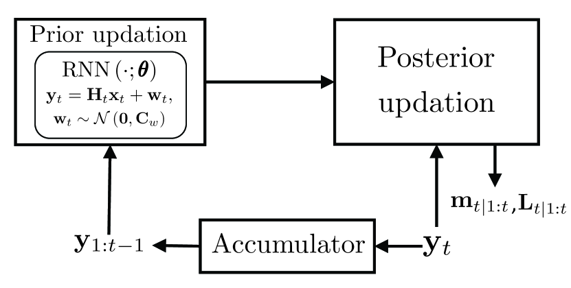
(a)

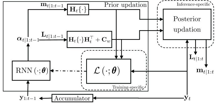
(b)

Figure 1: DANSE architecture. (a) Simple block diagram for inference. (b) Detailed diagram. The dash-dotted line represents the gradient flow during the training phase, solid lines indicate information flow during training/inference. Training/inference-specific blocks are shown within dashed borders. The ‘Accumulator’ block collects observations recursively.

To learn the parameters of DANSE, we have a training dataset $\mathcal{D}$ comprised of $N$ time-series measurements as $\mathcal{D}=\{\mathbf{y}^{(i)}_{1:T^{(i)}}\}_{i=1}^{N}$. Here $\mathbf{y}^{(i)}_{1:T^{(i)}}=\mathbf{y}_{1}^{(i)},\mathbf{y}_{2}^{(i)},\ldots,\mathbf{y}_{T^{(i)}}^{(i)}$ is the $i^{th}$ time-series measurements of length $T^{(i)}$. Note that $T^{(i)}$ can vary across time-series measurements (unequal lengths). Since we do not have access to the corresponding state sequences, $\mathcal{D}$ is unlabelled and the learning problem is unsupervised.

II-B DANSE System

DANSE is model-free. It only has access to $\mathcal{D}$. DANSE is data-driven and seeks to have analytical tractability like model-driven methods. So, to use data and the measurement system together, a prior-posterior system setup needs to be developed where the prior comes from data and the posterior follows the constraint of the linear measurement system. Principally, we model the unknown prior probability distribution $p\left(\mathbf{x}_{t}|\mathbf{y}_{1:t-1}\right)$ as a Gaussian distribution parameterized using an RNN. At time instant $t$, an RNN recursively uses the input sequence $\mathbf{y}_{1:t-1}$ and provides the parameters of the Gaussian prior as the output, collectively denoted as $\boldsymbol{\alpha}_{t|1:t-1}$. An RNN has its parameters $\boldsymbol{\theta}$, thus its output also depends on $\boldsymbol{\theta}$. To indicate this, we write $\boldsymbol{\alpha}_{t|1:t-1}\triangleq\boldsymbol{\alpha}_{t|1:t-1}(\boldsymbol{\theta})$. A simple block diagram of the Bayesian estimation as the inference of DANSE is shown in Fig. 1(a).

Bayesian State Estimation (Solution of T1)

The task is to obtain current state posterior $p(\mathbf{x}_{t}|\mathbf{y}_{1},\ldots,\mathbf{y}_{t-1},\mathbf{y}_{t})=p(\mathbf{x}_{t}|\mathbf{y}_{1:t})$, and the time-series posterior $p(\mathbf{x}_{1:t}|\mathbf{y}_{1:t})$. The prior distribution $p\left(\mathbf{x}_{t}|\mathbf{y}_{1:t-1}\right)$ and the observation distribution $p\left(\mathbf{y}_{t}|\mathbf{x}_{t}\right)$ are shown below in (6).

$$\begin{array}[]{c}\mathrm{Prior:}\,p(\mathbf{x}_{t}|\mathbf{y}_{1:t-1})\!=\!\mathcal{N}(\mathbf{x}_{t};\mathbf{m}_{t|1:t-1}(\boldsymbol{\theta}),\mathbf{L}_{t|1:t-1}(\boldsymbol{\theta})),\\ \text{ such that }\{\mathbf{m}_{t|1:t-1}(\boldsymbol{\theta}),\mathbf{L}_{t|1:t-1}(\boldsymbol{\theta})\}\triangleq\boldsymbol{\alpha}_{t|1:t-1}(\boldsymbol{\theta}),\\ \boldsymbol{\alpha}_{t|1:t-1}\left(\boldsymbol{\theta}\right)=\mathrm{RNN}(\mathbf{y}_{1:t-1};\boldsymbol{\theta}).\\ \mathrm{Observation:}\,p(\mathbf{y}_{t}|\mathbf{x}_{t})=\mathcal{N}(\mathbf{y}_{t};\mathbf{H}_{t}\mathbf{x}_{t},\mathbf{C}_{w}).\end{array}$$ (6)

Here, $\mathbf{m}_{t|1:t-1}(\boldsymbol{\theta})\in\mathbb{R}^{m}$ and $\mathbf{L}_{t|1:t-1}(\boldsymbol{\theta})\in\mathbb{R}^{m\times m}$ denote the mean and covariance matrix of the Gaussian prior distribution, respectively. The mean and covariance depend on RNN parameters $\boldsymbol{\theta}$, and hence we show it in notations. We use $\mathbf{L}_{t|1:t-1}(\boldsymbol{\theta})$ as a diagonal covariance matrix for ease of practical implementation. Then, using the ‘completing the square’ approach [33, Chap. 2], the posterior distribution of the current state $p\left(\mathbf{x}_{t}|\mathbf{y}_{1:t}\right)$ is obtained in closed-form as

$$\begin{array}[]{rl}&p(\mathbf{x}_{t}|\mathbf{y}_{1:t})=\mathcal{N}(\mathbf{x}_{t};\mathbf{m}_{t|1:t}(\boldsymbol{\theta}),\mathbf{L}_{t|1:t}(\boldsymbol{\theta})),\\ &\mathbf{m}_{t|1:t}(\boldsymbol{\theta})=\mathbf{m}_{t|1:t-1}(\boldsymbol{\theta})+\mathbf{K}_{t|1:t-1}\boldsymbol{\varepsilon}_{t},\\ &\mathbf{L}_{t|1:t}(\boldsymbol{\theta})=\mathbf{L}_{t|1:t-1}(\boldsymbol{\theta})-\mathbf{K}_{t|1:t-1}\mathbf{R}_{\varepsilon}\mathbf{K}_{t|1:t-1}^{\top},\\ \end{array}$$ (10)

where the second equation in (10) is obtained using the Woodbury matrix identity/matrix inversion lemma, with

$$\begin{array}[]{l}\mathbf{K}_{t|1:t-1}\triangleq\mathbf{L}_{t|1:t-1}(\boldsymbol{\theta})\mathbf{H}_{t}^{\top}\mathbf{R}_{\varepsilon}^{-1},\\ \mathbf{R}_{\varepsilon}\triangleq\mathbf{H}_{t}\mathbf{L}_{t|1:t-1}\left(\boldsymbol{\theta}\right)\mathbf{H}_{t}^{\top}+\mathbf{C}_{w},\,\,\mathrm{and}\\ {\boldsymbol{\varepsilon}}_{t}\triangleq\mathbf{y}_{t}-\mathbf{H}_{t}\mathbf{m}_{t|1:t-1}(\boldsymbol{\theta}).\end{array}$$ (11)

A point estimate is $\mathbf{m}_{t|1:t}({\boldsymbol{\theta}})$, that provides a practical mean-square-error (MSE) performance as $\mathbb{E}\{\|\mathbf{x}_{t}-\mathbf{m}_{t|1:t}(\boldsymbol{\theta})\|_{2}^{2}\}$.

Finally, using (10) we can estimate the closed-form posterior of the time series $\mathbf{x}_{1:t}$ given $\mathbf{y}_{1:t}$, as

$$\begin{array}[]{rl}p\!\left(\mathbf{x}_{1:t}|\mathbf{y}_{1:t}\right)\!\!\!\!\!\!&=p\left(\mathbf{x}_{t}|\mathbf{y}_{1:t},\mathbf{x}_{1:t-1}\right)p\left(\mathbf{x}_{1:t-1}|\mathbf{y}_{1:t}\right)\\ &=p\left(\mathbf{x}_{t}|\mathbf{y}_{1:t}\right)p\left(\mathbf{x}_{1:t-1}|\mathbf{y}_{1:t-1}\right)\\ &=\,\prod_{\tau=1}^{t}p\left(\mathbf{x}_{\tau}|\mathbf{y}_{1:\tau}\right)\\ &=\,\prod_{\tau=1}^{t}\!\mathcal{N}(\mathbf{x}_{\tau};\mathbf{m}_{{\tau}|1:{\tau}}(\boldsymbol{\theta}),\mathbf{L}_{{\tau}|1:{\tau}}(\boldsymbol{\theta}))\\ &\triangleq p\!\left(\mathbf{x}_{1:t}|\mathbf{y}_{1:t};\boldsymbol{\theta}\right).\end{array}$$ (17)

Here we introduced the notation $p(\mathbf{x}_{1:t}|\mathbf{y}_{1:t};\boldsymbol{\theta})$ to show the dependency of $p(\mathbf{x}_{1:t}|\mathbf{y}_{1:t})$ on $\boldsymbol{\theta}$.

We note two interesting issues - a similarity and a difference. Firstly, in (10) we notice a similarity with the standard KF update equations for the posterior [11, Chap. 5]. Secondly, we note a difference. While KF has a Gaussian progression of the posterior to the prior of the next time point, there is no such thing in DANSE. The parameters $\boldsymbol{\alpha}_{t|1:t-1}\left(\boldsymbol{\theta}\right)$ of the prior distribution are obtained from the RNN and the RNN does not use any process model that leads to a Gaussian progression.

II-C Unsupervised learning of DANSE

In this subsection, we address how to learn the RNN parameters $\boldsymbol{\theta}$ in DANSE using the training dataset $\mathcal{D}=\{\mathbf{y}^{(i)}_{1:T^{(i)}}\}_{i=1}^{N}$. We first express $p(\mathbf{y}_{t}|\mathbf{y}_{1:t-1})$ as follows -

$$\begin{array}[]{l}p(\mathbf{y}_{t}|\mathbf{y}_{1:t-1})\\ =\displaystyle\int_{\mathbf{x}_{t}}p(\mathbf{y}_{t}|\mathbf{x}_{t})p(\mathbf{x}_{t}|\mathbf{y}_{1:t-1})\,d\mathbf{x}_{t}\\ =\!\!\displaystyle\int_{\mathbf{x}_{t}}\!\!\mathcal{N}(\mathbf{y}_{t};\!\mathbf{H}_{t}\mathbf{x}_{t},\!\mathbf{C}_{w}\!)\,\mathcal{N}(\mathbf{x}_{t};\!\mathbf{m}_{t|1:t-1}(\boldsymbol{\theta}),\!\mathbf{L}_{t|1:t-1}(\boldsymbol{\theta})\!)\,d\mathbf{x}_{t}\!\!\!\!\\ =\mathcal{N}(\mathbf{y}_{t};\mathbf{H}_{t}\mathbf{m}_{t|1:t-1}(\boldsymbol{\theta}),\mathbf{C}_{w}+\mathbf{H}_{t}\mathbf{L}_{t|1:t-1}(\boldsymbol{\theta})\mathbf{H}_{t}^{\top})\\ \triangleq p(\mathbf{y}_{t}|\mathbf{y}_{1:t-1};\boldsymbol{\theta}).\end{array}$$ (23)

In the third line of the above equation, we used (6). Here we introduced the notation $p(\mathbf{y}_{t}|\mathbf{y}_{1:t-1};\boldsymbol{\theta})$ to show the dependency of $p(\mathbf{y}_{t}|\mathbf{y}_{1:t-1})$ on $\boldsymbol{\theta}$. Now, using the chain rule of probability, we can write

$$\begin{array}[]{l}p\left(\mathbf{y}_{1:T}\right)\triangleq p\left(\mathbf{y}_{1:T};\boldsymbol{\theta}\right)=\prod_{t=1}^{T}p\left(\mathbf{y}_{t}|\mathbf{y}_{1:t-1};\boldsymbol{\theta}\right),\,\mathrm{and}\\ p\left(\mathbf{y}^{(i)}_{1:T^{(i)}}\right)\triangleq p\left(\mathbf{y}^{(i)}_{1:T^{(i)}};\boldsymbol{\theta}\right)=\prod_{t=1}^{T^{(i)}}p\left(\mathbf{y}_{t}^{(i)}|\mathbf{y}_{1:t-1}^{(i)};\boldsymbol{\theta}\!\right)\!\!.\end{array}$$ (26)

Therefore, using the dataset $\mathcal{D}$, the maximum-likelihood based unsupervised learning (optmization) problem is

$$\begin{array}[]{l}\max_{\boldsymbol{\theta}}\log\prod_{i=1}^{N}\prod_{t=1}^{T^{(i)}}p\left(\mathbf{y}_{t}^{(i)}|\mathbf{y}_{1:t-1}^{(i)};{\boldsymbol{\theta}}\right)\\ =\max_{\boldsymbol{\theta}}\sum_{i=1}^{N}\sum_{t=1}^{T^{(i)}}\log p\left(\mathbf{y}_{t}^{(i)}|\mathbf{y}_{1:t-1}^{(i)};{\boldsymbol{\theta}}\right)\\ =\min_{\boldsymbol{\theta}}-\sum_{i=1}^{N}\sum_{t=1}^{T^{(i)}}\log p\left(\mathbf{y}_{t}^{(i)}|\mathbf{y}_{1:t-1}^{(i)};{\boldsymbol{\theta}}\right)\\ =\min_{\boldsymbol{\theta}}\sum_{i=1}^{N}\mathcal{L}\left(\mathbf{y}^{(i)}_{1:T^{(i)}};{\boldsymbol{\theta}}\right),\\ \end{array}$$ (31)

with the loss function denoted as $\mathcal{L}$, defined as $\mathcal{L}\left(\mathbf{y}^{(i)}_{1:T^{(i)}};{\boldsymbol{\theta}}\right)\triangleq-\sum_{t=1}^{T^{(i)}}\log p\left(\mathbf{y}_{t}^{(i)}|\mathbf{y}_{1:t-1}^{(i)};{\boldsymbol{\theta}}\right)$. Dropping the superscipt $(i)$, we can write

$$\begin{array}[]{l}\mathcal{L}\left(\mathbf{y}_{1:T};{\boldsymbol{\theta}}\right)\triangleq-\sum_{t=1}^{T}\log p\left(\mathbf{y}_{t}|\mathbf{y}_{1:t-1};{\boldsymbol{\theta}}\right)\\ =\sum_{t=1}^{T}\frac{1}{2}\|\mathbf{y}_{t}-\mathbf{H}_{t}\mathbf{m}_{t|1:t-1}(\boldsymbol{\theta})\|_{\left(\!\mathbf{C}_{w}+\mathbf{H}_{t}\mathbf{L}_{t|1:t-1}(\boldsymbol{\theta})\mathbf{H}_{t}^{\top}\!\right)^{\!\!-1}}^{2}\!\!\\ +\frac{n}{2}\log 2\pi+\frac{1}{2}\log\text{det}\left(\mathbf{C}_{w}+\mathbf{H}_{t}\mathbf{L}_{t|1:t-1}(\boldsymbol{\theta})\mathbf{H}_{t}^{\top}\right)\!\!.\end{array}$$ (35)

The optimization problem (31) can be further formulated as a Bayesian learning problem if we have a suitable prior of ${\boldsymbol{\theta}}$ as $p({\boldsymbol{\theta}})$. For example, if we use an isotropic Gaussian prior, then we have a standard $\ell_{2}$-norm based regularization in the form of $\|\boldsymbol{\theta}\|_{2}^{2}$ penalty. If we use Laplacian prior then we have a sparsity-promoting $\ell_{1}$-norm based penalty in the form of $\|\boldsymbol{\theta}\|_{1}$. The optimization in (31) uses a gradient-descent to learn the parameters $\boldsymbol{\theta}$. Therefore, we can comment that the solution approach that we used for the unsupervised learning is a suitable combination of Bayesian learning (or maximum-likelihood learning) and data-driven learning (of RNNs). Fig. 1(b) shows a detailed block diagram to depict the training and inference-specific blocks.

Note that we do not need to use variational inference (VI) to optimize (31). VI is an approximate Bayesian learning method, used in dynamical variational autoencoders (DVAEs) [22, 23, 24]. Instead, we endeavor direct optimization of (31) using gradient-descent, without approximations.

On the choice of RNNs

We can use prominent RNNs, such as GRUs [17] and LSTMs [18]. Here we used GRUs owing to their simplicity and popularity [34, 35]. Specifically, for modeling the mean vector and diagonal covariance matrix of the parameterized Gaussian prior in (6), we transformed the latent state of the GRU using feed-forward networks. We used rectified linear unit (ReLU) activations to model the non-negative variances.

II-D Bayesian Forecasting

We have mentioned the Bayesian forecasting problem in section II-A, as task T2. After unsupervised learning of DANSE, note that (6) and (23) provide the solution of the forecasting problem T2.

II-E Empirical estimation-performance limit of DANSE

For a model-free process, it is non-trivial to provide a standard performance limit, for example, quantifying the minimum-mean-square-error (MMSE) performance and comparing it with the practical performance of an estimator. Instead, we can use a pragmatic approach, where we use a supervised learning setup, find a performance limit, and compare. Note that the approach provides an empirical performance limit. The reason for using such a performance limit is an educated guess: an unsupervised learning-based method like DANSE can not perform better than a supervised learning-based method.

We now explain how to provide the empirical performance limit in the supervised learning setup. Let us assume we have access to a labelled dataset $\overline{\mathcal{D}}\!=\!\left\{\left(\mathbf{x}^{(i)}_{1:T^{(i)}},\mathbf{y}^{(i)}_{1:T^{(i)}}\right)\right\}_{i=1}^{N}$. Note that $\mathcal{D}\!\subset\!\overline{\mathcal{D}}$. Both $\mathcal{D}$ and $\overline{\mathcal{D}}$ have $N$ training data samples. Dropping the superscript $(i)$, we have state-and-measurement data-pair $\left(\mathbf{x}_{1:T},\mathbf{y}_{1:T}\right)$, that includes $\left(\mathbf{x}_{1:t},\mathbf{y}_{1:t}\right),t=1,2,\ldots,T$.

There can be many ways to design a supervised learning setup. Let us design a setup where we find parameters of the RNN of DANSE for the Bayesian state estimation $p(\mathbf{x}_{t}|\mathbf{y}_{1:t})$. Using (10) and (17), denoting $p\left(\mathbf{x}_{t}|\mathbf{y}_{1:t}\right)\triangleq p\left(\mathbf{x}_{t}|\mathbf{y}_{1:t};{{\boldsymbol{\theta}}}\right)$ in (17), and using the dataset $\overline{\mathcal{D}}$, the maximum-likelihood based supervised learning (optimization) problem is

$$\begin{array}[]{rl}\boldsymbol{\theta}_{s}\!\!\!\!&=\arg\max_{\boldsymbol{\theta}}\log\prod_{i=1}^{N}\prod_{t=1}^{T^{(i)}}p\left(\mathbf{x}_{t}^{(i)}|\mathbf{y}_{1:t}^{(i)};{\boldsymbol{\theta}}\right)\\ &=\arg\max_{\boldsymbol{\theta}}\sum_{i=1}^{N}\sum_{t=1}^{T^{(i)}}\log p\left(\mathbf{x}_{t}^{(i)}|\mathbf{y}_{1:t}^{(i)};{\boldsymbol{\theta}}\right)\\ &=\arg\min_{\boldsymbol{\theta}}-\sum_{i=1}^{N}\sum_{t=1}^{T^{(i)}}\log p\left(\mathbf{x}_{t}^{(i)}|\mathbf{y}_{1:t}^{(i)};{\boldsymbol{\theta}}\right)\\ &=\arg\min_{\boldsymbol{\theta}}\sum_{i=1}^{N}\overline{\mathcal{L}}\left(\left(\mathbf{x}^{(i)}_{1:T^{(i)}},\mathbf{y}^{(i)}_{1:T^{(i)}}\right);{\boldsymbol{\theta}}\right),\\ \end{array}$$ (40)

with the loss function denoted as $\overline{\mathcal{L}}$, defined as $\overline{\mathcal{L}}\left(\left(\mathbf{x}^{(i)}_{1:T^{(i)}},\mathbf{y}^{(i)}_{1:T^{(i)}}\right);{\boldsymbol{\theta}}\right)\!\triangleq-\sum_{t=1}^{T^{(i)}}\log p\left(\mathbf{x}_{t}^{(i)}|\mathbf{y}_{1:t}^{(i)};{\boldsymbol{\theta}}\right)$. Dropping the superscript $(i)$, we can write

$$\begin{array}[]{l}\overline{\mathcal{L}}\left(\left(\mathbf{x}_{1:T},\mathbf{y}_{1:T}\right);{\boldsymbol{\theta}}\right)\triangleq-\sum_{t=1}^{T}\log p\left(\mathbf{x}_{t}|\mathbf{y}_{1:t};{\boldsymbol{\theta}}\right)\\ =\sum_{t=1}^{T}\frac{1}{2}\|\mathbf{x}_{t}-\mathbf{m}_{t|1:t}(\boldsymbol{\theta})\|_{\mathbf{L}^{-1}_{t|1:t}(\boldsymbol{\theta})}^{2}\\ +\frac{m}{2}\log 2\pi+\frac{1}{2}\log\text{det}\left(\mathbf{L}_{t|1:t}(\boldsymbol{\theta})\right).\end{array}$$ (44)

Using gradient descent we address the optimization problem (40), and find $\boldsymbol{\theta}_{s}$; here we use the superscript ‘$s$’ to denote ‘supervised’. A point estimate is $\mathbf{m}_{t|1:t}({\boldsymbol{\theta}_{s}})$, that provides an empirical MSE performance limit.

II-F On causal and anti-causal usages

While we developed DANSE maintaining causality, it is amenable for designing anti-causal methods. For example, at time point $t$, we can use inputs $\mathbf{y}_{t+\tau},\tau\geq 1$ along with $\mathbf{y}_{1:t-1}$ for providing a prior and then find a posterior with the use of $\mathbf{y}_{t}$. The method can be even fully anti-causal. That means we can use $\mathbf{y}_{t+1:T}$ as an input to provide a prior and then find a posterior with the use of $\mathbf{y}_{t}$. There can be several possibilities for using measurements in causal and anti-causal manners. In this article, we focus on state estimation maintaining causality.

III Experiments and Results

We now perform simulation studies and compare DANSE vis-à-vis a few other Bayesian methods, such as model-based KF, EKF, UKF, and the hybrid method KalmanNet. We use unsupervised KalmanNet [29] to have a fair comparison with DANSE. The five methods that we compare experimentally have the following properties.

1. KF - Knows the linear process model. Optimum for a linear process model. Knows the measurement system (1).

2. EKF - Knows the linearized form of the nonlinear process model based on a first-order Taylor series expansion. Knows the measurement system.

3. UKF - Knows the nonlinear process model, and uses numerical techniques such as sigma-point methods. Knows the measurement system.

4. Unsupervised KalmanNet - Knows the linearized form of a nonlinear process model, like EKF, but does not need to know the process noise. Knows the measurement system, but does not use the measurement noise statistics. Uses an unlabelled training dataset $\mathcal{D}$.

5. DANSE - Does not know the process model. Knows the measurement system. Uses the training dataset $\mathcal{D}$.

Note, we do not perform any direct comparison with data-driven methods such as DVAE or RNN, since they are not readily applicable to the state estimation problems with the knowledge of measurement systems. But we compare with KalmanNet as it is directly applicable, and it uses attributes from both model-driven and data-driven approaches.

For the experiments, our setup is inspired by the KalmanNet papers [28, 29]. We experiment with measurement and state sequences generated from two different SSMs with additive white Gaussian noise. We first start with a linear SSM to show a proof-of-concept experiment on how DANSE performs in comparison with the optimal system - the KF. Then we investigate two non-linear SSMs - a Lorenz attractor as used in [29] and a Chen attractor [32, 36]. For an experiment, we have a training dataset, mentioned before, as $\mathcal{D}=\{\mathbf{y}^{(i)}_{1:T^{(i)}}\}_{i=1}^{N}$, and a testing dataset $\mathcal{D}_{\text{test}}=\left\{\left(\mathbf{x}^{(j)}_{1:T_{\text{test}}^{(j)}},\mathbf{y}^{(j)}_{1:T_{\text{test}}^{(j)}}\right)\right\}_{j=1}^{\!N_{\text{test}}}$. Denoting the estimated state as $\hat{\mathbf{x}}_{t}$, we use the averaged normalized-mean-squared-error (NMSE) as the performance measure, defined below.

$$\text{NMSE}=\frac{1}{N_{\text{test}}}\sum_{j=1}^{N_{\text{test}}}10\log_{10}\frac{\sum_{t=1}^{T^{(j)}}\|\mathbf{x}_{t}^{(j)}-\hat{\mathbf{x}}_{t}^{(j)}\|_{2}^{2}}{\sum_{t=1}^{T^{(j)}}\|\mathbf{x}_{t}^{(j)}\|_{2}^{2}}.$$ (45)

The estimated state $\hat{\mathbf{x}}_{t}$ corresponds to the posterior mean for all the five state estimation methods considered in this experimental study.

III-A Training, performance measures, and RNN architecture

We find the architectures for the RNN and the feed-forward networks used in RNN experimentally by grid search and cross-validation. For the RNN, we use a one-layer GRU model with 30 hidden nodes. The feed-forward networks are modeled as shallow networks with a single hidden layer having $32$ hidden nodes. We implement DANSE in Python and PyTorch [37] and train the architecture using GPU support . The training algorithm uses a mini-batch gradient descent with a batch size of $64$. The optimizer chosen is Adam [38] with an adaptive learning rate set at a starting value $10^{-2}$ and is decreased step-wise by a factor of $0.9$ every ${1/6}^{\text{th}}$ of the maximum number of training epochs. The maximum number of training epochs is set at $2000$, and early stopping is used to avoid overfitting. In the case of optimizing the empirical performance limit using (40), we again use Adam as the optimizer with an adaptive learning rate starting at $5\times 10^{-3}$.

III-B On implementation of the competing methods

The performances of DANSE are compared with baseline methods that estimate the state sequence from the measurement data. First, we used a naive, least squares (LS) estimator, which gives estimated state $\hat{\mathbf{x}}_{t}$ in closed-form as

$$\hat{\mathbf{x}}_{t}=\left(\mathbf{H}_{t}^{\top}\mathbf{C}_{w}^{-1}\mathbf{H}_{t}\right)^{-1}\mathbf{H}_{t}^{\top}\mathbf{C}_{w}^{-1}\mathbf{y}_{t}$$ (46)

We implemented KF, EKF, and UKF using PyTorch and FilterPy [39]. We used the implementation of the unsupervised KalmanNet from [29] for our experimental study.

III-C Linear SSM

To compare DANSE with the optimal KF, we first perform a proof-of-concept experiment with a linear SSM. The experiment is motivated by [29, 28]. The linear SSM model is as follows:

$$\mathbf{x}_{t} =\mathbf{F}\mathbf{x}_{t-1}+\mathbf{e}_{t}\in\mathbb{R}^{2},$$ (47)

$$\mathbf{y}_{t} =\mathbf{H}\mathbf{x}_{t}+\mathbf{w}_{t}\in\mathbb{R}^{2},$$

where $t=1,2,\dots,T$, $\mathbf{F}\in\mathbb{R}^{2\times 2}$, $\mathbf{H}\in\mathbb{R}^{2\times 2}$, $\mathbf{e}_{t}\sim\mathcal{N}(\boldsymbol{0},\mathbf{C}_{e})$ is the white Gaussian process noise variable with $\mathbf{C}_{e}=\sigma_{e}^{2}\mathbf{I}_{2}$, and $\mathbf{w}_{t}\sim\mathcal{N}(\boldsymbol{0},\mathbf{C}_{w})$ is the white Gaussian measurement noise with $\mathbf{C}_{w}=\sigma_{w}^{2}\mathbf{I}_{2}$ ($\mathbf{I}_{2}$ denotes the $2\times 2$ identity matrix). The matrices $\mathbf{F},\mathbf{H}$ are time-invariant, where $\mathbf{H}$ is an identity matrix and $\mathbf{F}$ is a scaled upper triangular matrix.

We simulate (47) to create the training and testing data, and then compare DANSE with the standard KF and LS. LS does not use time-wise correlation. KF knows the signal model. All of them know the measurement model and measurement noise statistics. We train DANSE using a training dataset $\mathcal{D}$, where $N=500,T=500$ (all the training sequences are of the same length). We varied the signal-to-measurement noise ratio (SMNR) from $-10$ to $30$ dB, with a fixed $\sigma_{e}^{2}=-10\text{ dB}$. The SMNR is calculated on $\mathcal{D}_{\text{test}}$ as

$$\begin{array}[]{lr}\text{SMNR}\!\!\!\!\!\!&=\!\!\frac{1}{N_{\text{test}}}\!\!\sum\limits_{j=1}^{N_{\text{test}}}\!\!10\log_{10}\!\!\left(\frac{\sum_{t=1}^{T_{\text{test}}^{(j)}}\mathbb{E}\{\|\mathbf{H}\mathbf{x}_{t}^{(j)}-\mathbb{E}\{\mathbf{H}\mathbf{x}_{t}^{(j)}\}\|_{2}^{2}\}}{\text{tr}\left(\mathbf{C}_{w}\right)}\right)\\ \!\!&=\!\!\frac{1}{N_{\text{test}}}\!\!\sum\limits_{j=1}^{N_{\text{test}}}\!\!10\log_{10}\!\!\left(\frac{\sum_{t=1}^{T_{\text{test}}^{(j)}}\mathbb{E}\{\|\mathbf{H}\mathbf{x}_{t}^{(j)}-\mathbb{E}\{\mathbf{H}\mathbf{x}_{t}^{(j)}\}\|_{2}^{2}\}}{n\sigma_{w}^{2}}\right)\\ \end{array}$$ (50)

We evaluate all the methods on the same test set. For the test set, we have $N_{\text{test}}=100$ trajectories with $T_{\text{test}}=1000$. We deliberately use the longer test-sample trajectory than the training-sample trajectory to check whether DANSE can generalize to longer trajectory lengths. The variation of NMSE versus SMNR is shown in Fig. 2. We can observe that DANSE performs close to the optimal KF. Note that the gap between KF and DANSE consistently increases as SMNR decreases. This is a consistent result for learning with noisy data. Moreover, we observed empirically that the gap between KF and DANSE decreases with the use of more training data samples $N$ of $\mathcal{D}$. This is consistent with the behavior we expected, and we do not elaborate further on the sample complexity for the linear case.

Figure 2: Plot of NMSE (in dB) vs SMNR (in dB) for the linear SSM. Here, KF performance is the lower bound and LS is a possible upper bound.

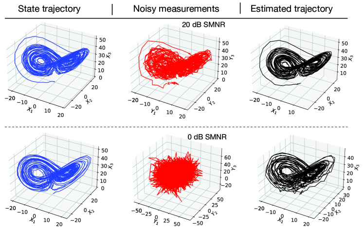
Figure 3: State estimation for Lorenz attractor using DANSE, at 20 dB and 0 dB SMNR with $\mathbf{H}_{t}=\mathbf{I}_{3}$. The first row is for 20 dB SMNR, and the second row is for 0 dB SMNR. The left column shows the true state trajectories, the middle column shows noisy measurement trajectories, and the right column shows the estimated state trajectories. Note that, in unsupervised learning, the training dataset $\mathcal{D}$ comprises of $N$ such ‘red colored’ noisy measurement trajectories.

Figure 4: Performance comparison of all methods for the Lorenz attractor SSM, including the empirical performance limit.

III-D Lorenz attractor SSM (nonlinear SSM)

Next, we experiment with a non-linear SSM - the Lorenz attractor SSM [31]. Similarly to [28, 40], the SSM is in a discretized form as

$$\mathbf{x}_{t}=\mathbf{F}_{t}(\mathbf{x}_{t-1})\mathbf{x}_{t-1}+\mathbf{e}_{t}\in\mathbb{R}^{3},$$ (51)

where $\mathbf{e}_{t}\sim\mathcal{N}(\boldsymbol{0},\mathbf{C}_{e})$ with $\mathbf{C}_{e}=\sigma_{e}^{2}\mathbf{I}_{3}$, and

$$\mathbf{F}_{t}(\mathbf{x}_{t-1})=\exp\left(\begin{bmatrix}-10&10&0\\ 28&-1&-x_{t-1,1}\\ 0&x_{t-1,1}&-\frac{8}{3}\\ \end{bmatrix}\Delta\right),$$ (52)

with the step-size $\Delta=0.02\text{ seconds}$. In our simulations, we use a finite-Taylor series approximation of $5^{th}$ order for (52). The measurement model is

$$\mathbf{y}_{t}=\mathbf{H}_{t}\mathbf{x}_{t}+\mathbf{w}_{t}\in\mathbb{R}^{3}.$$ (53)

We use $\mathbf{H}_{t}=\mathbf{I}_{3}$. The measurement noise is $\mathbf{w}_{t}\sim\mathcal{N}(\boldsymbol{0},\mathbf{C}_{w})$ with $\mathbf{C}_{w}=\sigma_{w}^{2}\mathbf{I}_{3}$, while $\sigma_{e}^{2}$ corresponds to $-10$ dB. For this SSM, we compare DANSE vis-à-vis EKF, UKF, and unsupervised KalmanNet. We train DANSE using dataset $\mathcal{D}$ with $N=500$, $T=1000$, while for KalmanNet we use $\mathcal{D}$ with $N=500,T=100$ [29]. For KalmanNet, the reason for using $T=100$ is due to some convergence issues that we encountered during the training of KalmanNet using longer trajectories. We evaluate all the methods on the same test set $\mathcal{D}_{\text{test}}$ with $N_{\text{test}}=100$ and $T_{\text{test}}=2000$. Like the linear SSM case, we test on longer trajectories than the training.

III-D1 State estimation

With a focus on the state estimation task, we start with a visual illustration of the DANSE performance. Fig. 3 shows two random instances of Lorenz attractor SSM trajectories, their noisy measurements, and corresponding estimates using DANSE. The top row is SMNR = 20 dB and the bottom row for SMNR = 0 dB. Note that, at a particular SMNR, the training dataset $\mathcal{D}$ is comprised of such kind of noisy measurement trajectories. Even at SMNR = 0 dB, without knowing the process model, DANSE is able to extract meaningful information from the noisy input and then provide a reasonable estimate of the state trajectory.

Figure 5: Visualization of mean and uncertainty of the estimated posterior $x_{t,2}$ given $\mathbf{y}_{1:t}$, that means $p(x_{t,2}|\mathbf{y}_{1:t})$, for the Lorenz attractor SSM. We have $\sigma_{e}^{2}$ corresponding to $-10$ dB, and $\text{SMNR}=0$ dB. The shaded areas in red and yellow show the uncertainty of the estimate by one-sigma-point using DANSE and UKF, respectively.

Then we show a performance comparison (NMSE versus SMNR) for all the competing methods in Fig. 4. In the figure, we also show the empirical performance limit of DANSE, mentioned in subsection II-E. We can see that, across different SMNR values, DANSE provides competitive performances. We note an interesting trend in the region where SMNR is high. While performances of all the methods saturate in the higher SMNR region, there exists a large gap between the empirical performance limit and DANSE performances. This hints at future opportunities for further improvements of DANSE.

We now visually show the uncertainty of estimates using a single-dimensional trajectory. In Fig. 4, at 0 dB SMNR, UKF is found to be the most competitive to DANSE in terms of NMSE. This motivates us to qualitatively compare the state estimates of UKF and DANSE. In Fig. 5, we show the visualization of the estimated posterior of $x_{2}$-dimension of three-dimensional Lorenz attractor SSM. The shaded regions represent the uncertainties of the estimates by one-sigma-point (standard deviation of the posterior). It is clear that DANSE has less uncertainty than the UKF.

III-D2 Forecasting

In this subsection, we show forecasting results visually for the Lorenz attractor SSM. We show uncertainty of forecasting $p(\mathbf{y}_{t+1}|\mathbf{y}_{1:t})$ across single-dimensional trajectories. We use the same experimental conditions as Fig. 5 in the previous experiment, and show the second-dimension of the three-dimensional trajectories, i.e. $p\left(y_{t,2}|\mathbf{y}_{1:t-1}\right)$. UKF and DANSE are compared in relation to the true trajectories. Fig. 6 shows the forecasting of ${y}_{t,2}$, i.e. $p({y}_{t,2}|\mathbf{y}_{1:t-1})$ at 0 dB SMNR. The shaded regions represent the uncertainty of the estimates by one-sigma-point. Note that $\mathbf{y}_{t}$ is difficult to forecast at the low SMNR = 0 dB, as $\mathbf{y}_{t}$ has a significant amount of noise component.

Figure 6: Visualization of the mean and uncertainty of the forecast of ${y}_{t,2}$ given $\mathbf{y}_{1:t-1}$, that means $p({y}_{t,2}|\mathbf{y}_{1:t-1})$, for the Lorenz attractor SSM. We have $\sigma_{e}^{2}$ corresponding to $-10$ dB, and $\text{SMNR}=0$ dB. The shaded areas in red and yellow show the uncertainty of the forecast by one-sigma-point using DANSE and UKF respectively.

III-D3 Remark

Using the above experiments and visualizations, we demonstrate that the DANSE is competitive. The results show that it is possible to design an unsupervised learning-based data-driven method to estimate the non-linear state of a process-free model using linear measurements.

III-E On training data amount and mismatched conditions

Given the encouraging performance of DANSE, two important questions arise: (a) How much training data is required for DANSE to perform well? We do not have any theoretical results for this question. Instead, we deliberate on the question using experiments. (b) All the experiments so far mentioned are conducted in matched training-and-testing conditions. What will happen in mismatched conditions? This question is central to a standard robustness study. We deliberate on these two questions in the following.

Figure 7: Effect of increasing the number of samples $N$ on the performance of DANSE and KalmanNet. The black-bordered marker indicates the value of $N=500$ used throughout the paper for training DANSE and KalmanNet.

III-E1 On the training data amount

We wish to study the effect of the number of sample trajectories required for training DANSE. For this study, we vary the number of sample trajectories - $N$ in $\mathcal{D}$, which means the size of $\mathcal{D}$. We keep the length of a trajectory $T$ fixed at $T=100$ and perform the experiments. We also have a fixed $\sigma_{e}^{2}=-10$ dB, and $\text{SMNR}=10$ dB. We train DANSE at varying $N$ and evaluate on a test dataset $\mathcal{D}_{\text{test}}$ with $N_{\text{test}}=100,T_{\text{test}}=2000$ at the same SMNR and $\sigma_{e}^{2}$ as for training. The results are shown in Fig. 7. We see that DANSE requires a certain number of training sample trajectories $N$ to provide good performance. The performance improves with an approximately linear trend with respect to $\log_{10}N$ for small $N$ and then shows a saturation trend. The performance improvement indicates an (approximate) exponential trend with respect to $N$ – a power law behavior. This reminds us of performance-versus-resource, such as distortion-rate curves in source coding. Note that we include KalmanNet’s behavior in the same figure and find that it can be trained with fewer data. We believe that the reason is – KalmanNet knows the process SSM. On the other hand, DANSE requires more data as it does not know the process SSM.

III-E2 On mismatched conditions for robustness study

Here we study two cases as follows:

Mismatched process

We study the robustness of training-based methods - DANSE and KalmanNet - for a mismatched process. We generate a mismatched process by varying the process noise $\sigma_{e}^{2}$. A change in the process noise reflects a drift in the original SSM. Keeping SMNR = 10 dB, we train DANSE and KalmanNet using $\sigma_{e}^{2}=-10$ dB and then test at varying $\sigma_{e}^{2}$. An increase in $\sigma_{e}^{2}$ amounts to an increase in uncertainty (or randomness) in Lorenz SSM. The performances are shown in Fig. 8. We observe that the performances of both DANSE and KalmanNet deteriorate with increasing $\sigma_{e}^{2}$.

Figure 8: Performance in case of mismatched process noise for the Lorenz attractor. At a fixed $\text{SMNR}=10$ dB, DANSE and KalmanNet are trained using $\sigma_{e}^{2}=-10$ dB, and then tested at varying $\sigma_{e}^{2}$.

Mismatched measurement noise

Figure 9: Performance in case of mismatched measurement noise for the Lorenz attractor SSM. The ‘DANSE - Mismatched’ and ‘KalmanNet - Mismatched’ were trained at $\text{SMNR}=10$ dB, $\sigma_{e}^{2}=-10$ dB, and then tested at varying SMNR.

Now, we investigate the effect of a mismatch in the additive measurement noise $\mathbf{w}_{t}$ on the performances of DANSE and KalmanNet. The change in the measurement noise during testing reflects a change in the measurement setup. Keeping $\sigma_{e}^{2}$ fixed corresponding to $-10$ dB, we train DANSE and KalmanNet using $\text{SMNR}=10$ dB and then test at varying SMNR. The performances are shown in Fig. 9. We can observe that DANSE shows a degradation in performance at mismatched SMNR (i.e. except at $\text{SMNR}=10$ dB that corresponds to the matched training condition). DANSE is more susceptible than the KalmanNet to mismatched measurement noise.

Remark

The susceptibility of DANSE to mismatched training and testing conditions is perhaps due to its lack of a-priori knowledge about the process. An educated guess to address the susceptibility is via a standard approach of multi-condition training, for example, if we train DANSE using training data comprised of several SMNRs and/or several process noise strengths. We do not further investigate the design of robust DANSE in this article. The design of robust DANSE using multi-condition training remains as part of future work.

III-F A limitation of DANSE (for subsampled measurements)

While we developed DANSE in an unsupervised manner and shown its competitive performance against several methods, a question can be as follows: is there any limitation of DANSE? Is there a scenario where DANSE has a high limitation, but the other competitors do well? Here we demonstrate such a scenario experimentally. We perform an experiment for subsampled measurements in the case of Lorenz attractor SSM. We implement this using a random measurement matrix $\mathbf{H}_{t}=\mathbf{H}$ of size $2\times 3$ with i.i.d. entries sampled from $\mathcal{N}\left(0,1\right)$. This is a case of subsampling with $\frac{2}{3}$ ratio ($\frac{n}{m}=\frac{2}{3}$). Note that this is an under-determined estimation and learning problem. We then generate training data using this random matrix $\mathbf{H}$ and train DANSE appropriately. The performance is shown in Fig. 10, where DANSE fails to perform. On the other hand, EKF, UKF, and KalmanNet do well. Our guess is that DANSE suffers since it has no a-priori knowledge of the process. Therefore, it lacks appropriate regularization for solving the under-determined estimation problem. We do not further investigate the design of DANSE for subsampled measurements in this article. This remains a part of future work.

Figure 10: Effect of subsampled measurements using $\mathbf{H}_{t}=\mathbf{H}$ as a $2\times 3$ Gaussian random matrix. DANSE shows a limitation.

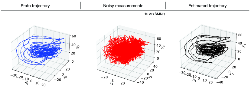
Figure 11: State estimation for the Chen attractor using DANSE, at 10 dB SMNR with $\mathbf{H}_{t}=\mathbf{I}_{3}$. The true state trajectory at $\sigma_{e}^{2}=-10$ dB is shown in the left, noisy measurements at 10 dB SMNR in the middle, and the estimated trajectory in the right.

III-G Experiments for another nonlinear SSM - Chen attractor

So far we have shown results for one nonlinear SSM - the Lorenz attractor SSM. A natural question is how DANSE performs for other nonlinear SSMs. Or a non-trivial question can be: what will be the complexity level of a nonlinear SSM such that DANSE can show a good performance? As we do not have any theoretical arguments at this point to answer the questions, we conduct experiments for another chaotic attractor, called Chen attractor [32, 36]. The experiment is to demonstrate the behavior of DANSE in the case of another nonlinear SSM.

For the Chen attractor SSM, we performed experiments similar to the Lorenz attractor SSM in section III-D. Instead of reporting several results, we show DANSE performance visually in Fig. 11 for one randomly chosen trajectory at $\text{SMNR}=10$ dB. The figure helps to visualize the state trajectory for the Chen attractor SSM, the corresponding measurement trajectory at $10$ dB SMNR, and finally the estimated trajectory using DANSE. In this experiment, the NMSE of DANSE is found to be $-22.40\pm 0.29$ dB, while for EKF and UKF the NMSE values are roughly the same and equal to $-22.73\pm 0.27$ dB. Hence, for the Chen attractor SSM, DANSE also shows competitive performance. The Chen attractor model that we use for our simulation study is shown in appendix -A.

IV Conclusions and future scopes

Experimental results show that the proposed DANSE is competitive. The development of DANSE concludes that it is possible to design an unsupervised learning-based data-driven method to estimate the non-linear state of a model-free process using a training dataset of linear measurements. In addition, a major conclusion is that the amount of training data is a key factor contributing to good performance. The NMSE performance improvement with the size of training data follows a power law behavior. It also shows that unsupervised learning faces difficulty to handle an under-determined system for a model-free process (the sub-sampled measurement system that we investigated).

Several questions remain open. (a) How to handle nonlinear measurements instead of linear measurements? (b) How to handle unknown Gaussian measurement noise statistics, for example, the unknown covariance matrix? (c) How to handle non-Gaussian measurement noise statistics? (d) How to handle mismatched training-and-testing conditions for robustness? (e) How to handle data-limited scenarios, for example, a limited amount of training data, and/or sub-sampled measurements? We hope that the above questions will pose new research challenges in the future.

-A Chen attractor model

As in the case of the Lorenz attractor SSM in section III-D, the Chen attractor SSM [32] is in a discretized form as

$$\mathbf{x}_{t}=\mathbf{F}^{\prime}_{t}(\mathbf{x}_{t-1})\mathbf{x}_{t-1}+\mathbf{e}_{t}\in\mathbb{R}^{3},$$ (54)

where $\mathbf{e}_{t}\sim\mathcal{N}(\boldsymbol{0},\mathbf{C}_{e})$ with $\mathbf{C}_{e}=\sigma_{e}^{2}\mathbf{I}_{3}$, and

$$\mathbf{F}^{\prime}_{t}(\mathbf{x}_{t-1})=\exp\left(\begin{bmatrix}-35&35&0\\ -7&28&-x_{t-1,1}\\ 0&x_{t-1,1}&-{3}\\ \end{bmatrix}\Delta^{\prime}\right),$$ (55)

with the step-size $\Delta^{\prime}=0.002\text{ seconds}$. The discretization is performed similarly as in [40]. We note that in the case of the Chen attractor [32], we require a smaller step size $\Delta^{\prime}$, to avoid instability during simulation. In our simulations, we use a finite-Taylor series approximation of $5^{th}$ order for (55). The measurement model is linear, where $\mathbf{H}_{t}=\mathbf{I}_{3}$ in the measurement model (1). The measurement noise is $\mathbf{w}_{t}\sim\mathcal{N}(\boldsymbol{0},\mathbf{C}_{w})$ with $\mathbf{C}_{w}=\sigma_{w}^{2}\mathbf{I}_{3}$, while $\sigma_{e}^{2}$ corresponds to $-10$ dB.

References

- [1] R.E. Kalman, “New results in linear filtering and prediction theory,” J. Basic Eng., vol. 83, pp. 95–108, 1961.
- [2] R.E. Kalman, “A new approach to linear filtering and prediction problems,” Trans. ASME, D, vol. 82, pp. 35–44, 1960.
- [3] M. Gruber, “An approach to target tracking,” Tech. Rep., MIT Lexington Lincoln Lab, 1967.
- [4] S.J. Julier and J.K. Uhlmann, “Unscented filtering and nonlinear estimation,” Proceedings of the IEEE, vol. 92, no. 3, pp. 401–422, 2004.
- [5] M. S. Arulampalam, S. Maskell, N. Gordon, and T. Clapp, “A tutorial on particle filters for online nonlinear/non-gaussian bayesian tracking,” IEEE Transactions on Signal Processing, vol. 50, no. 2, pp. 174–188, 2002.
- [6] A. Ghosh, A. Honoré, and S. Chatterjee, “DANSE: Data-driven Non-linear State Estimation of Model-free Process in Unsupervised Bayesian Setup,” in European Signal Processing Conference (EUSIPCO), 2023 (To appear).
- [7] H. Guo, D. Cao, H. Chen, C. Lv, H. Wang, and S. Yang, “Vehicle dynamic state estimation: State of the art schemes and perspectives,” IEEE/CAA Journal of Automatica Sinica, vol. 5, no. 2, pp. 418–431, 2018.
- [8] M. Athans, R. Wishner, and A. Bertolini, “Suboptimal state estimation for continuous-time nonlinear systems from discrete noisy measurements,” IEEE Transactions on Automatic Control, vol. 13, no. 5, pp. 504–514, 1968.
- [9] E.A. Wan and R. Van Der Merwe, “The unscented Kalman filter for nonlinear estimation,” in Proceedings of the IEEE 2000 Adaptive Systems for Signal Processing, Communications, and Control Symposium (Cat. No. 00EX373). IEEE, 2000, pp. 153–158.
- [10] I. Arasaratnam and S. Haykin, “Cubature Kalman filters,” IEEE Transactions on Automatic Control, vol. 54, no. 6, pp. 1254–1269, 2009.
- [11] D. Simon, Optimal state estimation: Kalman, , and nonlinear approaches, John Wiley & Sons, 2006.
- [12] P. Kaminski, A. Bryson, and S. Schmidt, “Discrete square root filtering: A survey of current techniques,” IEEE Transactions on Automatic Control, vol. 16, no. 6, pp. 727–736, 1971.
- [13] P.G. Park and T. Kailath, “New square-root algorithms for kalman filtering,” IEEE Transactions on Automatic Control, vol. 40, no. 5, pp. 895–899, 1995.
- [14] R. Van Der Merwe and E.A. Wan, “The square-root unscented Kalman filter for state and parameter-estimation,” in IEEE International Conference on Acoustics, Speech, and Signal Processing (ICASSP). Proceedings (Cat. No. 01CH37221). IEEE, 2001, vol. 6, pp. 3461–3464.
- [15] A. Doucet, N. De Freitas, N. J. Gordon, et al., Sequential Monte Carlo methods in practice, vol. 1, Springer, 2001.
- [16] S.C. Patwardhan, S. Narasimhan, P. Jagadeesan, B. Gopaluni, and S.L. Shah, “Nonlinear Bayesian state estimation: A review of recent developments,” Control Engineering Practice, vol. 20, no. 10, pp. 933–953, 2012.
- [17] K. Cho, B. van Merriënboer, D. Bahdanau, and Y. Bengio, “On the properties of neural machine translation: Encoder–decoder approaches,” in Proc. of workshop, SSST-8, 2014, pp. 103–111.
- [18] S. Hochreiter and J. Schmidhuber, “Long short-term memory,” Neural computation, vol. 9, no. 8, pp. 1735–1780, 1997.
- [19] N. Yadaiah and G. Sowmya, “Neural network based state estimation of dynamical systems,” in IEEE international joint conference on neural network proceedings. IEEE, 2006, pp. 1042–1049.
- [20] L. Xu and R. Niu, “EKFNet: Learning system noise statistics from measurement data,” in IEEE International Conference on Acoustics, Speech and Signal Processing (ICASSP). IEEE, 2021, pp. 4560–4564.
- [21] H. Coskun, F. Achilles, R. DiPietro, N. Navab, and F. Tombari, “Long short-term memory Kalman filters: Recurrent neural estimators for pose regularization,” in Proceedings of the IEEE International Conference on Computer Vision, 2017, pp. 5524–5532.
- [22] L. Girin, S. Leglaive, X. Bie, J. Diard, T. Hueber, and X. Alameda-Pineda, “Dynamical variational autoencoders: A comprehensive review,” Foundations and Trends in Machine Learning, vol. 15, no. 1-2, pp. 1–175, 2021.
- [23] M. Fraccaro, S. Kamronn, U. Paquet, and O. Winther, “A disentangled recognition and nonlinear dynamics model for unsupervised learning,” Advances in NeurIPS, vol. 30, 2017.
- [24] R. Krishnan, U. Shalit, and D. Sontag, “Structured inference networks for nonlinear state space models,” in Proceedings of the AAAI Conference on Artificial Intelligence, 2017, vol. 31.
- [25] M. Karl, M. Soelch, J. Bayer, and P. van der Smagt, “Deep Variational Bayes Filters: Unsupervised Learning of State Space Models from Raw Data,” in International Conference on Learning Representations, 2017.
- [26] P. Becker, H. Pandya, G. Gebhardt, C. Zhao, J.C. Taylor, and G. Neumann, “Recurrent Kalman networks: Factorized inference in high-dimensional deep feature spaces,” in International Conference on Machine Learning. PMLR, 2019, pp. 544–552.
- [27] A. Vaswani, N. Shazeer, N. Parmar, J. Uszkoreit, L. Jones, A. N Gomez, Ł. Kaiser, and I. Polosukhin, “Attention is all you need,” Advances in NeurIPS, vol. 30, 2017.
- [28] G. Revach, N. Shlezinger, X. Ni, A. L. Escoriza, R.J.G. Van Sloun, and Y.C. Eldar, “KalmanNet: Neural network aided Kalman filtering for partially known dynamics,” IEEE Transactions on Signal Processing, vol. 70, pp. 1532–1547, 2022.
- [29] G. Revach, N. Shlezinger, T. Locher, X. Ni, R.J.G. van Sloun, and Y.C. Eldar, “Unsupervised learned Kalman filtering,” in 2022 30th European Signal Processing Conference (EUSIPCO). IEEE, 2022, pp. 1571–1575.
- [30] X. Ni, G. Revach, N. Shlezinger, R.J.G. van Sloun, and Y.C. Eldar, “RTSNet: Deep learning aided Kalman smoothing,” in IEEE International Conference on Acoustics, Speech and Signal Processing (ICASSP). IEEE, 2022, pp. 5902–5906.
- [31] E.N. Lorenz, “Deterministic nonperiodic flow,” Journal of atmospheric sciences, vol. 20, no. 2, pp. 130–141, 1963.
- [32] G. Chen and T. Ueta, “Yet another chaotic attractor,” International Journal of Bifurcation and chaos, vol. 9, no. 07, pp. 1465–1466, 1999.
- [33] C. M. Bishop and N. M. Nasrabadi, Pattern recognition and machine learning, vol. 4, Springer, 2006.
- [34] J. Chung, C. Gulcehre, K. Cho, and Y. Bengio, “Empirical evaluation of gated recurrent neural networks on sequence modeling,” in NeurIPS 2014 Workshop on Deep Learning, December 2014, 2014.
- [35] M. Ravanelli, P. Brakel, M. Omologo, and Y. Bengio, “Light gated recurrent units for speech recognition,” IEEE Transactions on Emerging Topics in Computational Intelligence, vol. 2, no. 2, pp. 92–102, 2018.
- [36] S. Čelikovskỳ and G. Chen, “On the generalized lorenz canonical form,” Chaos, Solitons & Fractals, vol. 26, no. 5, pp. 1271–1276, 2005.
- [37] A. Paszke et al., “PyTorch: An imperative style, high-performance deep learning library,” Advances in NeurIPS, vol. 32, 2019.
- [38] D.P. Kingma and J. Ba, “Adam: A method for stochastic optimization,” in 3rd International Conference on Learning Representations (ICLR), 2015.
- [39] R. Labbe, “FilterPy - Kalman and Bayesian filters in Python,” URL: https://filterpy.readthedocs.io/en/latest/, 2018.
- [40] V. Garcia Satorras, Z. Akata, and M. Welling, “Combining generative and discriminative models for hybrid inference,” Advances in NeurIPS, vol. 32, 2019.