Fractals from Regular Behaviours

Abstract

We are interested in connections between the theory of fractal sets obtained as attractors of iterated function systems and process calculi. To this end, we reinterpret Milner’s expressions for processes as contraction operators on a complete metric space. When the space is, for example, the plane, the denotations of fixed point terms correspond to familiar fractal sets. We give a sound and complete axiomatization of fractal equivalence, the congruence on terms consisting of pairs that construct identical self-similar sets in all interpretations. We further make connections to labelled Markov chains and to invariant measures. In all of this work, we use important results from process calculi. For example, we use Rabinovich’s completeness theorem for trace equivalence in our own completeness theorem. In addition to our results, we also raise many questions related to both fractals and process calculi.

1 Introduction

Hutchinson noticed in [16] that many familiar examples of fractals can be captured as the set-wise fixed-point of a finite family of contraction (i.e., distance shrinking) operators on a metric space. He called these spaces (strictly) self-similar, since the intuition behind the contraction operators is that they are witnesses for the appearance of the fractal in a proper (smaller) subset of itself. For example, the famous Sierpiński gasket is the unique nonempty compact subset of the plane left fixed by the union of the three operators $\sigma_{a},\sigma_{b},\sigma_{c}:\mathbb{R}^{2}\to\mathbb{R}^{2}$ in Figure 1. The Sierpiński gasket is a scaled-up version of each of its thirds.

$\begin{gathered}\leavevmode\hbox to55.57pt{\vbox to15.55pt{\text{[drawing]}}}\\ \\ \sigma_{a}\begin{bmatrix}r\\ s\end{bmatrix}=\begin{bmatrix}\frac{1}{2}r+\frac{1}{4}\\ \frac{1}{2}s+\frac{\sqrt{3}}{4}\end{bmatrix}\qquad\sigma_{b}\begin{bmatrix}r\\ s\end{bmatrix}=\begin{bmatrix}\frac{1}{2}r\\ \frac{1}{2}s\end{bmatrix}\\ \sigma_{c}\begin{bmatrix}r\\ s\end{bmatrix}=\begin{bmatrix}\frac{1}{2}r+\frac{1}{2}\\ \frac{1}{2}s\end{bmatrix}\end{gathered}$

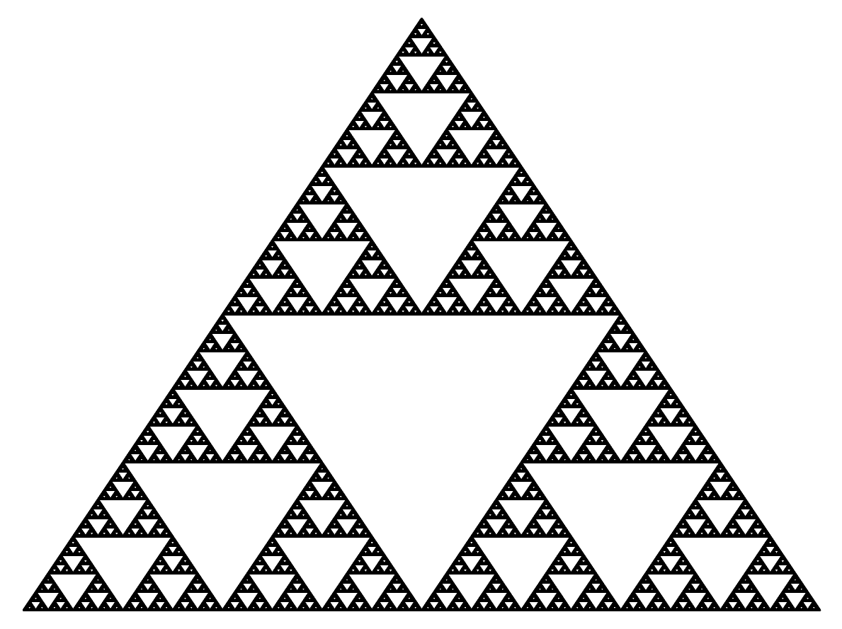
Figure 1: The Sierpiński gasket is the unique nonempty compact subset $\mathbf{S}$ of $\mathbf{R}^{2}$ such that $\mathbf{S}=\sigma_{a}(\mathbf{S})\cup\sigma_{b}(\mathbf{S})\cup\sigma_{c}(\mathbf{S})$. Each of its points corresponds to a stream emitted by the state $x$.

The self-similarity of Hutchinson’s fractals hints at an algorithm for constructing them: Each point in a self-similar set is the limit of a sequence of points obtained by applying the contraction operators one after the other to an initial point. In the Sierpiński gasket, the point $(1/4,\sqrt{3}/4)$ is the limit of the sequence

$$p,\ \sigma_{b}(p),\ \sigma_{b}\sigma_{a}(p),\ \sigma_{b}\sigma_{a}\sigma_{a}(p),\ \sigma_{b}\sigma_{a}\sigma_{a}\sigma_{a}(p),\ \dots$$ (1)

where the initial point $p$ is an arbitrary element of $\mathbf{R}^{2}$ (note that $\sigma_{b}$ is applied last). Hutchinson showed in [16] that the self-similar set corresponding to a given family of contraction operators is precisely the collection of points obtained in the manner just described. The limit of the sequence in (1) does not depend on the initial point $p$ because $\sigma_{a},\sigma_{b},\sigma_{c}$ are contractions. Much like digit expansions to real numbers, every stream of $a$’s, $b$’s, and $c$’s corresponds to a unique point in the Sierpiński gasket, as we have seen in (1). The point $(1/4,\sqrt{3}/4)$, for example, corresponds to the stream $(b,a,a,a,\dots)$ ending in an infinite sequence of $a$’s. Conversely, every point in the Sierpiński gasket comes from (in general more than one) corresponding stream.

From a computer science perspective, the languages of streams considered by Hutchinson are the traces observed by one-state labelled transition systems, like the one in Figure 1. We investigate whether one could achieve a similar effect with languages of streams obtained from labelled transition systems having more than one state. Observe, for example, Figure 2. These twisted versions of the Sierpiński gasket are constructed from the streams emitted by the two-state labelled transition system in Figure 2, starting from the states $x$ and $y$ respectively.

Each point in a twisted Sierpiński gasket corresponds to a stream of $a$’s, $b$’s, and $c$’s, but not every stream corresponds to a point in the set: The limit corresponding to the stream $(a,c,a,b,a,a,a,\dots)$ emitted by the state $x$ is $p=(19/32,11\sqrt{3}/32)$, for example, and this point does not appear in either of the twisted Sierpinski gaskets generated by $x$ or $y$.

$\begin{gathered}\leavevmode\hbox to94.96pt{\vbox to39.41pt{\text{[drawing]}}}\\ \begin{aligned} \sigma_{a}\begin{bmatrix}r\\ s\end{bmatrix}&=\begin{bmatrix}\frac{1}{2}r+\frac{1}{4}\\ \frac{1}{2}s+\frac{\sqrt{3}}{4}\end{bmatrix}\\ \sigma_{b}\begin{bmatrix}r\\ s\end{bmatrix}&=\begin{bmatrix}\frac{r}{2}\\ \frac{s}{2}\end{bmatrix}\\ \sigma_{c}\begin{bmatrix}r\\ s\end{bmatrix}&=\begin{bmatrix}\frac{r}{2}+\frac{1}{2}\\ \frac{s}{2}\end{bmatrix}\end{aligned}\end{gathered}$

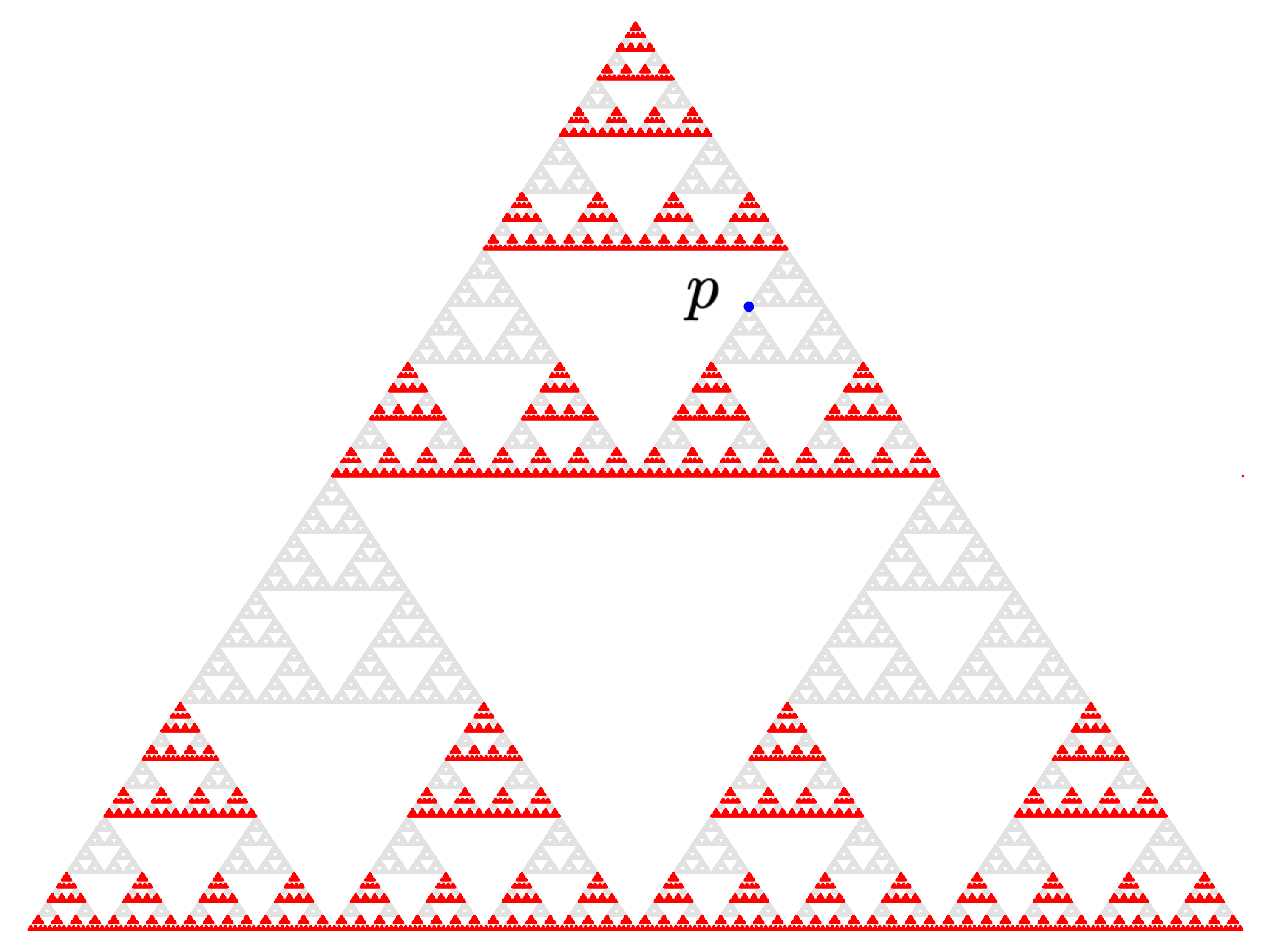
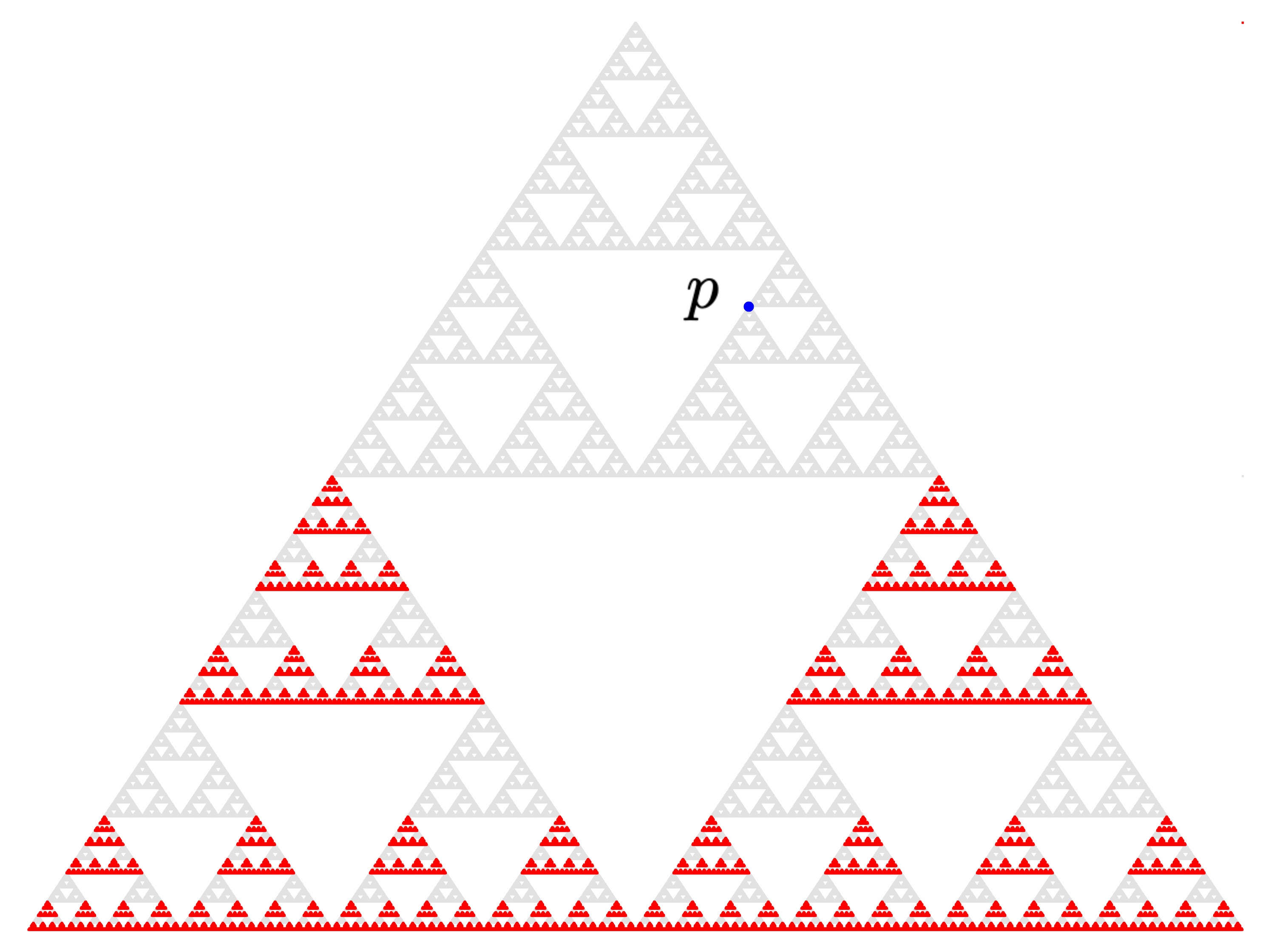
Generated by $x$. Generated by $y$.

Figure 2: Twisted Sierpińksi gaskets, depicted in red, and $p=(\frac{19}{32},\frac{11\sqrt{3}}{32})$. In the construction of the set generated by $x$, $\sigma_{b}$ and $\sigma_{c}$ are applied twice to a single copy of $\sigma_{a}$ applied to the set. This has the effect of systematically removing the “top” part of the Sierpiński gasket from its bottom thirds. The set generated by $y$ is the union of $\sigma_{b}$ and $\sigma_{c}$ applied to the set generated by $x$.

In analogy with the theory of regular languages, we call the fractals generated by finite labelled transition systems regular subfractals, and give a logic for deciding if two labelled transition systems represent the same recipe under all interpretations of the labels, allowing both the underlying space and the chosen contractions to vary. By identifying points in the fractal set generated by a labelled transition system with traces observed by the labelled transition system, it is reasonable to suspect that two labelled transition systems represent equivalent fractal recipes—i.e., they represent the same fractal under every interpretation—if and only if they are trace equivalent. This is the content of Theorem 4.4, which allows us to connect the theory of fractal sets to mainstream topics in computer science.

Labelled transition systems are a staple of theoretical computer science, especially in the area of process algebra [2], where a vast array of different notions of equivalence and axiomatization problems have been studied. We specifically use a syntax introduced by Milner in [28] to express labelled transition systems as terms in an expression language with recursion. This leads us to a fragment of Milner’s calculus consisting of just the terms that constitute recipes for fractal constructions. Using a logic of Rabinovich [32] for deciding trace equivalence in Milner’s calculus, we obtain a complete axiomatization of fractal recipe equivalence.

In his study of self-similar sets, Hutchinson also makes use of probability measures supported on self-similar sets, called invariant measures. Each invariant measure is specified by a probability distribution on the set of contractions generating its support. In the last technical section of the paper, we adapt the construction of invariant measures to a probabilistic version of labelled transition systems called labelled Markov chains, which allows us to give a measure-theoretic semantics to terms in a probabilistic version of Milner’s specification language, the calculus introduced by Stark and Smolka [35]. Our measure-theoretic semantics of probabilistic process terms can be seen as a generalization of the trace measure semantics of Kerstan and König [17]. We offer a sound axiomatization of equivalence under this semantics and pose completeness as an open problem.

In sum, the contributions of this paper are as follows.

• In Section 3, we give a fractal recipe semantics to process terms using a generalization of iterated function systems.

• In Section 4, we show that two process terms agree on all fractal interpretations if and only if they are trace equivalent. This implies that fractal recipe equivalence is decidable for process terms, and it allows us to derive a complete axiomatization of fractal recipe equivalence from Rabinovich’s axiomatization [32] of trace equivalence of process terms.

• We adapt the fractal semantics of process terms to the probabilistic setting in Section 5. We furthermore show that probabilistic fractal recipe equivalence coincides with Kerstan and König’s notion of trace measure equivalence [17].

• Finally, we propose an axiomatization of probabilistic fractal recipe equivalence in Section 6. We prove that our axioms are sound with respect to our semantics and pose completeness as an open problem.

We start with a brief overview of trace semantics in process algebra and Rabinovich’s Theorem (Theorem 2.10) in Section 2.

2 Labelled Transition Systems and Trace Semantics

Labelled transition systems are a widely used model of nondeterminism. Given a fixed finite set $A$ of action labels, a labelled transition system (LTS) is a pair $(X,\alpha)$ consisting of a set $X$ of states (also called the state space) and a transition function $\alpha:X\to\mathcal{P}(A\times X)$. We generally write $x\mathrel{\raisebox{-1.0pt}{$\xrightarrow{a}$}}_{\alpha}y$ if $(a,y)\in\alpha(x)$, or simply $x\mathrel{\raisebox{-1.0pt}{$\xrightarrow{a}$}}y$ if $\alpha$ is clear from context, and say that $x$ emits $a$ and transitions to $y$.

Given a state $x$ of an LTS $(X,\alpha)$, we write $\langle x\rangle_{\alpha}$ for the LTS obtained by restricting the relations $\mathrel{\raisebox{-1.0pt}{$\xrightarrow{a}$}}$ to the set of states reachable from $x$, meaning there exists a path of the form $x\mathrel{\raisebox{-1.0pt}{$\xrightarrow{a_{1}}$}}x_{1}\mathrel{\raisebox{-1.0pt}{$\xrightarrow{}$}}\cdots\mathrel{\raisebox{-1.0pt}{$\xrightarrow{}$}}x_{n-1}\mathrel{\raisebox{-1.0pt}{$\xrightarrow{a_{n}}$}}x_{n}$. We refer to $\langle x\rangle_{\alpha}$ as either the LTS generated by $x$, or the process starting at $x$. An LTS $(X,\alpha)$ is locally finite if $\langle x\rangle_{\alpha}$ is finite for every state $x$. The reader should note that there exist locally finite LTSs with infinite state spaces, and that one such LTS will be important in this paper.

Traces

In the context of the current work, nondeterminism occurs when a process branches into multiple threads that execute in parallel. Under this interpretation, to an outside observer (without direct access to the implementation details of an LTS), two processes that emit the same set of sequences of action labels are indistinguishable.

Formally, let $A^{*}$ be the set of finite words formed from the alphabet $A$. Given a state $x$ of an LTS $(X,\alpha)$, the set $\operatorname{tr}_{\alpha}(x)$ of traces emitted by $x$ is the set of words $a_{1}\cdots a_{n}\in A^{*}$ such that there is a path of the form $x\mathrel{\raisebox{-1.0pt}{$\xrightarrow{a_{1}}$}}x_{1}\mathrel{\raisebox{-1.0pt}{$\xrightarrow{a_{2}}$}}\cdots\mathrel{\raisebox{-1.0pt}{$\xrightarrow{a_{n-1}}$}}x_{n-1}\mathrel{\raisebox{-1.0pt}{$\xrightarrow{a_{n}}$}}x_{n}$ through $(X,\alpha)$. Given LTSs $(X,\alpha)$ and $(Y,\beta)$, states $x\in X$ and $y\in Y$ are called trace equivalent if $\operatorname{tr}_{\alpha}(x)=\operatorname{tr}_{\beta}(y)$. If the transition structure is clear from context, we drop it from the notation and write simply $\operatorname{tr}(x)$ for $\operatorname{tr}_{\alpha}(x)$. It should be noted that every trace language $\operatorname{tr}_{\alpha}(x)$ is prefix-closed, which for a language $L$ means that $w\in L$ whenever $wa\in L$ for some $a\in A$.

Trace equivalence is a well-documented notion of equivalence for processes [14, 4], and we shall see it in our work on fractals as well.

Definition 2.1.

A stream is an infinite sequence $(a_{1},a_{2},\dots)$ of letters from $A$. The set of streams is denoted $A^{\omega}$. A state $x$ in an LTS $(X,\alpha)$ emits a stream $(a_{1},\dots)$ if there is an infinite path of the form $x\mathrel{\raisebox{-1.0pt}{$\xrightarrow{a_{1}}$}}x_{1}\mathrel{\raisebox{-1.0pt}{$\xrightarrow{a_{2}}$}}\cdots\mathrel{\raisebox{-1.0pt}{$\xrightarrow{a_{n}}$}}x_{n}\mathrel{\raisebox{-1.0pt}{$\xrightarrow{a_{n+1}}$}}\cdots$ through $(X,\alpha)$. We write $\operatorname{str}_{\alpha}(x)$ for the set of streams emitted by $x$.

In our construction of fractals from LTSs, points are represented only by (infinite) streams. We therefore focus primarily on LTSs with the property that for all states $x$, $\operatorname{tr}(x)$ is precisely the set of finite prefixes of streams emitted by $x$. We refer to an LTS $(X,\alpha)$ satisfying this condition as productive. Productivity is equivalent to the absence of deadlock states, which are states with no outgoing transitions.

Lemma 2.2.

Let $(X,\alpha)$ be a finitely branching LTS. Then the following are equivalent:

1. $(X,\alpha)$ is productive, i.e., for any $x\in X$,

   $$\operatorname{tr}_{\alpha}(x) =\{a_{1}\dots a_{n}\in A^{*}\mid\exists(b_{1},\dots)\in\operatorname{str}_{\alpha}(x)\leavevmode\nobreak\ \text{such that}\leavevmode\nobreak\ b_{1}=a_{1},\dots,b_{n}=a_{n}\}$$ (2)

   $$\operatorname{str}_{\alpha}(x) =\{(a_{1},\dots)\in A^{\omega}\mid\forall n\in\mathbb{N},\leavevmode\nobreak\ a_{1}\cdots a_{n}\in\operatorname{tr}_{\alpha}(x)\}$$ (3)

2. For any $x\in X$, $\alpha(x)\neq\emptyset$.

Proof 2.3.

To see that 1 implies 2, observe that trivially, $\epsilon\in\operatorname{tr}_{\alpha}(x)$ for any $x\in X$ ($\epsilon$ is the empty word). This implies there is a stream $(a_{1},\dots)\in\operatorname{str}_{\alpha}(x)$ such that $\epsilon$ is an initial segment of $(a_{1},\dots)$, or in other words, $\operatorname{str}_{\alpha}(x)\neq\emptyset$. Hence, $\alpha(x)\neq\emptyset$, as $x$ emits a stream.

To see that 2 implies 1, assume $\alpha(x)\neq\emptyset$ for all $x\in X$. Then for any $x\in X$, a simple inductive argument shows that there are paths of arbitrary length starting from $x$. It follows from König’s lemma [19] (every infinite but finitely branching tree has an infinite branch) that there is therefore an infinite path starting at $x$. This allows us to argue as follows: To see (2), it suffices to show that $\operatorname{tr}_{\alpha}(x)$ is contained in the right hand side, as the reverse containment is clear. So, let $x\in X$ and suppose $a_{1}\dots a_{n}\in\operatorname{tr}_{\alpha}(x)$. Then there is a path $x\mathrel{\raisebox{-1.0pt}{$\xrightarrow{a_{1}}$}}\cdots\mathrel{\raisebox{-1.0pt}{$\xrightarrow{a_{n}}$}}x_{n}$, and by the observation above, there is an infinite path $x_{n}\mathrel{\raisebox{-1.0pt}{$\xrightarrow{a_{n+1}}$}}x_{n+1}\mathrel{\raisebox{-1.0pt}{$\xrightarrow{a_{n+1}}$}}\cdots$. Hence, $(a_{1},\dots,a_{n},a_{n+1},a_{n+2},\dots)\in\operatorname{str}_{\alpha}(x)$, as desired. This establishes (2).

To see (3), it suffices to see that $\operatorname{str}_{\alpha}(x)$ contains the right hand side, as the forward containment is clear. So, let $(a_{1},\dots)\in A^{\omega}$ such that for any $n\in\mathbb{N}$, $a_{1}\cdots a_{n}\in\operatorname{tr}_{\alpha}(x)$. We are going to use König’s lemma again: Let $x\in X$ and let $\mathfrak{P}$ be the set of all paths of the form $x\mathrel{\raisebox{-1.0pt}{$\xrightarrow{a_{1}}$}}\cdots\mathrel{\raisebox{-1.0pt}{$\xrightarrow{a_{n}}$}}x_{n}$. We define a tree tructure on $\mathfrak{P}$ as follows: Given $P_{1},P_{2}\in\mathfrak{P}$, write $P_{1}\to P_{2}$ if $P_{1}=(x\mathrel{\raisebox{-1.0pt}{$\xrightarrow{a_{1}}$}}\cdots\mathrel{\raisebox{-1.0pt}{$\xrightarrow{a_{n}}$}}x_{n})$ and $P_{2}=(x\mathrel{\raisebox{-1.0pt}{$\xrightarrow{a_{1}}$}}\cdots\mathrel{\raisebox{-1.0pt}{$\xrightarrow{a_{n}}$}}x_{n}\mathrel{\raisebox{-1.0pt}{$\xrightarrow{a_{n+1}}$}}x_{n+1})$ for some $x_{n+1}$. Then $(\mathfrak{P},\to)$ is an infinite but finitely branching tree, since every initial segment of $(a_{1},\dots)$ is in $\operatorname{tr}_{\alpha}(x)$ and $(X,\alpha)$ is finitely branching. By König’s lemma, there is an infinite path $P_{1}\to P_{2}\to\cdots$ in $(\mathfrak{P},\to)$. By definition, this means there is an infinite path $x\mathrel{\raisebox{-1.0pt}{$\xrightarrow{a_{1}}$}}x_{1}\mathrel{\raisebox{-1.0pt}{$\xrightarrow{a_{2}}$}}\cdots$ in $(X,\alpha)$. Hence, $(a_{1},\dots)\in\operatorname{str}_{\alpha}(x)$. This establishes (3).

As a direct consequence of Lemma 2.2, we have the following: If $(X,\alpha)$ is productive and finitely branching, and $x,y\in X$, then $\operatorname{str}_{\alpha}(x)=\operatorname{str}_{\alpha}(y)$ if and only if $\operatorname{tr}_{\alpha}(x)=\operatorname{tr}_{\alpha}(y)$.

Remark 2.4.

The finite branching condition is necessary in Lemma 2.2. For example, consider the LTSs in Figure 3. Between $x_{0}$ and $y_{0}$, only $y_{0}$ emits the stream $(a,b,a,b,a,b,\dots)$, despite both states emittting the trace language $\{(ab)^{n}\mid n\in\mathbb{N}\}$. This is possible because the LTS on the left is not finitely branching: Since $x_{0}\mathrel{\raisebox{-1.0pt}{$\xrightarrow{a}$}}x_{i,1}$ for every $i\in{\mathbb{N}}$, $x_{0}$ has infinitely many outgoing paths, but does not have an infinite outgoing path.

Figure 3: (A hedgehog model) The state $x_{0}$ emits every finite initial segment of $(a,b,a,b,a,b,\dots)$, but does not emit this stream. Therefore, $\operatorname{tr}(x_{0})=\operatorname{tr}(y_{0})$ and yet $\operatorname{str}(x_{0})\neq\operatorname{str}(y_{0})$.

Specification

We use the following language for specifying processes: Starting with a fixed countably infinite set $\{v_{1},v_{2},\dots\}$ of variables, the set of terms is given by the grammar

$$v\mid ae\mid e_{1}+e_{2}\mid\mu v\leavevmode\nobreak\ e$$

where $v$ is $v_{i}$ for some $i\in\mathbb{N}$, $a\in A$, and $e,e_{1},e_{2}$ are terms.

Intuitively, the process $ae$ emits $a$ and then turns into $e$, and $e_{1}+e_{2}$ is the process that nondeterministically branches into $e_{1}$ and $e_{2}$. The process $\mu v\leavevmode\nobreak\ e$ is like $e$, but with instances of $v$ that appear free in $e$ acting like goto expressions that return the process to $\mu v\leavevmode\nobreak\ e$.

Definition 1.

A (process) term is a term $e$ in which every occurrence of a variable $v$ appears both within the scope of a binder $\mu v\leavevmode\nobreak\ (-)$ ($e$ is closed) and within the scope of an action prefix operator $a(-)$ ($e$ is guarded). The set of process terms is written $\mathsf{Term}$. The set of process terms themselves form the LTS $(\mathsf{Term},\gamma)$ defined in Figure 4.

ae $\xrightarrow{a}$ e e_1 $\xrightarrow{a}$ fe_1 + e_2 $\xrightarrow{a}$ f e_2 $\xrightarrow{a}$ fe_1 + e_2 $\xrightarrow{a}$ f e[μv e/v] $\xrightarrow{a}$ fμv e $\xrightarrow{a}$ f

Figure 4: The relation ${\mathrel{\raisebox{-1.0pt}{$\xrightarrow{a}$}}}\subseteq\mathsf{Term}\times\mathsf{Term}$ defining $(\mathsf{Term},\gamma)$.

In Figure 4, we use the notation $e[g/v]$ to denote the expression obtained by replacing each free occurrence of $v$ in $e$ (one which does not appear within the scope of a $\mu v\leavevmode\nobreak\ (-)$ operator) with the expression $g$. Given $e\in\mathsf{Term}$, the process specified by $e$ is the LTS $\langle e\rangle_{\gamma}$.

Example 2.5.

Let $e=av$, and let $f=\mu v\leavevmode\nobreak\ e=\mu v\leavevmode\nobreak\ av$. Then $e[f/v]=af\mathrel{\raisebox{-1.0pt}{$\xrightarrow{a}$}}f$. By the last rule in Figure 4, $\mu v\leavevmode\nobreak\ e\mathrel{\raisebox{-1.0pt}{$\xrightarrow{a}$}}f=\mu v\leavevmode\nobreak\ e$. By looking at the other rules, we see that none apply. Hence, if $\mu v\leavevmode\nobreak\ e\mathrel{\raisebox{-1.0pt}{$\xrightarrow{b}$}}g$, then $b=a$ and $g=\mu v\leavevmode\nobreak\ e$. The upshot is that $\langle f\rangle_{\gamma}$, the process specified by $f$, is the one-point process which can perform $a$ but no other action: its state set is $\{f\}$, and $\gamma(f)=\{(a,f)\}$.

$$\leavevmode\hbox to62.32pt{\vbox to22.61pt{\text{[drawing]}}}\qquad\gamma(\mu v\leavevmode\nobreak\ av)=\gamma(a(\mu v\leavevmode\nobreak\ av))=\{(a,\mu v\leavevmode\nobreak\ av)\} \mu v\leavevmode\nobreak\ av a \mu v\leavevmode\nobreak\ av a$$

Remark 2.6.

The set of process terms, as we have named them, is the fragment of Milner’s fixed-point calculus from [28] consisting of only the terms that specify productive LTSs.

Labelled transition systems specified by process terms are finite and productive, and conversely, every finite productive process is trace-equivalent to some process term.

Lemma 2.7.

The LTS $(\mathsf{Term},\gamma)$ is productive and locally finite, i.e., for any $e\in\mathsf{Term}$, the set of terms reachable from $e$ in $(\mathsf{Term},\gamma)$ is finite. Conversely, if $x$ is a state in a productive and locally LTS $(X,\alpha)$, then there is a process term $e$ such that $\operatorname{tr}(e)=\operatorname{tr}_{\alpha}(x)$.

Proof 2.8.

Local finiteness of $(\mathsf{Term},\gamma)$ is [28, Proposition 5.1]. The proof that $(\mathsf{Term},\gamma)$ is productive is a routine induction on $e\in\mathsf{Term}$ that shows that $\gamma(e)\neq\emptyset$. The proof of the converse is a mild variation on Milner’s proof of [28, Theorem 5.7] with the added assumption that there are no unguarded variables $\vec{Y}$ in the given system of equations (see the cited proof). The lack of unguarded variables ensures that each expression $E_{i}$ of the solution is a process term in the last step.

Axiomatization of trace equivalence

Given an interpretation of process terms as states in an LTS, and given the notion of trace equivalence, one might ask if there is an algebraic or proof-theoretic account of trace equivalence of process terms. Rabinovich showed in [32] that a complete inference system for trace equivalence can be obtained by adapting earlier work of Milner [28]. The axioms of the complete inference system include equations like $e_{1}+e_{2}=e_{2}+e_{1}$ and $a(e_{1}+e_{2})=ae_{1}+ae_{2}$, which are intuitively true for trace equivalence.

To be more precise, given any function with domain $\mathsf{Term}$, say $\sigma:\mathsf{Term}\to Z$, call an equivalence relation $\sim$ sound with respect to $\sigma$ if $e\sim f$ implies $\sigma(e)=\sigma(f)$, and complete with respect to $\sigma$ if $\sigma(e)=\sigma(f)$ implies $e\sim f$. Then the smallest equivalence relation $\equiv$ on $\mathsf{Term}$ containing all the pairs derivable from the axioms and inference rules appearing in Figure 5 is sound and complete with respect to $\operatorname{tr}=\operatorname{tr}_{\gamma}\colon\mathsf{Term}\to\mathcal{P}(A^{*})$.

$$\begin{aligned} (\axiom{ID})\hskip 2.0pt&&e+e&\equiv e\\ (\axiom{CM})&&e_{2}+e_{1}&\equiv e_{1}+e_{2}\\ (\axiom{AS})\hskip 1.5pt&&e_{1}+(e_{2}+e_{3})&\equiv(e_{1}+e_{2})+e_{3}\\ (\axiom{DS})\hskip 1.3pt&&a(e_{1}+e_{2})&\equiv ae_{1}+ae_{2}\\ (\axiom{FP})\hskip 1.3pt&&\mu v\leavevmode\nobreak\ e&\equiv e[\mu v\leavevmode\nobreak\ e/v]\end{aligned}\qquad\begin{gathered}\begin{array}[]{r c}(\axiom{AE})&\mu w\leavevmode\nobreak\ e\equiv\mu v\leavevmode\nobreak\ e[v/w]\\ (\axiom{CN})&\infer{e_{1}\equiv f_{1}\leavevmode\nobreak\ \cdots\leavevmode\nobreak\ e_{n}\equiv f_{n}}{g[\vec{e}/\vec{v}]\equiv g[\vec{f}/\vec{v}]}\\ (\axiom{UA})&\infer{g\equiv e[g/v]}{g\equiv\mu v\leavevmode\nobreak\ e}\end{array}\end{gathered}$$

Figure 5: The axioms and rules of the provable equivalence relation in addition to those of equational logic (not shown). Here, $e,e_{i},f,f_{i},g\in\mathsf{Term}$ for all $i$. In $($, $g$ has precisely the free variables $v_{1},\dots,v_{n}$, and no variable that appears free in $f_{i}$ is bound in $g$ for any $i$. In $($, $v$ does not appear free in $e$.

Definition 2.9.

Given $e_{1},e_{2}\in\mathsf{Term}$, we say that $e_{1}$ and $e_{2}$ are provably equivalent if $e_{1}\equiv e_{2}$ can be derived from the axioms in Figure 5, and call $\equiv$ provable equivalence.

Theorem 2.10 (Rabinovich [32]).

Let $e_{1},e_{2}\in\mathsf{Term}$. Then $e_{1}\equiv e_{2}$ iff $\operatorname{tr}(e_{1})=\operatorname{tr}(e_{2})$.

Example 2.11.

Consider the processes specified by $e_{1}=\mu w\leavevmode\nobreak\ \mu v\leavevmode\nobreak\ (a_{1}a_{2}v+a_{1}a_{3}w)$ and $e_{2}=\mu v\leavevmode\nobreak\ (a_{1}(a_{2}v+a_{3}v))$ below.

$$\begin{gathered}\leavevmode\hbox to91.83pt{\vbox to60.5pt{\text{[drawing]}}}\qquad\qquad\leavevmode\hbox to52.73pt{\vbox to49.54pt{\text{[drawing]}}}\end{gathered} e_{1} a_{3}e_{1} a_{2}f_{1} f_{1} a_{1} a_{1} a_{3} a_{2} a_{1} a_{1} e_{2} a_{2}e_{2}+a_{3}e_{2} a_{1} a_{2},a_{3} e_{1} a_{3}e_{1} a_{2}f_{1} f_{1} a_{1} a_{1} a_{3} a_{2} a_{1} a_{1} e_{2} a_{2}e_{2}+a_{3}e_{2} a_{1} a_{2},a_{3}$$

The traces emitted by both $e_{1}$ and $e_{2}$ are those that alternate between $a_{1}$ and either $a_{2}$ or $a_{3}$. By Theorem 2.10, it should be possible to prove that $e_{1}\equiv e_{2}$. Indeed, this can be done as follows: Applying () to $e_{1}=\mu w\leavevmode\nobreak\ \mu v\leavevmode\nobreak\ (a_{1}a_{2}v+a_{1}a_{3}w)$, we start with

$$e_{1}=\mu w\leavevmode\nobreak\ \mu v\leavevmode\nobreak\ (a_{1}a_{2}v+a_{1}a_{3}w)\stackrel{{\scriptstyle(\axiom{FP})}}{{\equiv}}\mu v\leavevmode\nobreak\ (a_{1}a_{2}v+a_{1}a_{3}e_{1})$$

Applying $($ again, and then $($, we get

$$\mu v\leavevmode\nobreak\ (a_{1}a_{2}v+a_{1}a_{3}e_{1})\stackrel{{\scriptstyle(\axiom{FP})}}{{\equiv}}a_{1}a_{2}(\mu v\leavevmode\nobreak\ (a_{1}a_{2}v+a_{1}a_{3}e_{1}))+a_{1}a_{3}e_{1}\stackrel{{\scriptstyle(\axiom{CN})}}{{\equiv}}a_{1}a_{2}e_{1}+a_{1}a_{3}e_{1}$$

Applying () and using our substitution notation gives us

$$a_{1}a_{2}e_{1}+a_{1}a_{3}e_{1}\stackrel{{\scriptstyle(\axiom{DS})}}{{\equiv}}a_{1}(a_{2}e_{1}+a_{3}e_{1})=a_{1}(a_{2}v+a_{3}v)[e_{1}/v]$$

Thus, by applying (), we get

$$e_{1}\equiv a_{1}(a_{2}v+a_{3}v)[e_{1}/v]\stackrel{{\scriptstyle(\axiom{UA})}}{{\equiv}}\mu v\leavevmode\nobreak\ (a_{1}(a_{2}v+a_{3}v))=e_{2}$$

This shows that $e_{1}\equiv e_{2}$, as desired.

Rabinovich’s theorem tells us that, up to provable equivalence, our specification language consisting of process terms is really a specification language for languages of traces. In what follows, we are going to give an alternative semantics to process terms by using LTSs to generate fractal subsets of complete metric spaces. The main result of our paper is that these two semantics coincide: Two process terms are trace equivalent if and only if they generate the same fractals. This is the content of Sections 3 and 4 below.

3 Fractals from Labelled Transition Systems

In the Sierpiński gasket $\mathbf{S}$ from Figure 1, every point of $\mathbf{S}$ corresponds to a stream of letters from the alphabet $\{a,b,c\}$, and every stream corresponds to a unique point. To obtain the point corresponding to a particular stream $(a_{1},a_{2},a_{3},\dots)$ with each $a_{i}\in\{a,b,c\}$, start with any $p\in\mathbb{R}^{2}$ and compute the limit $\lim_{n\to\infty}\sigma_{a_{1}}\cdots\sigma_{a_{n}}(p)$. The point in the fractal corresponding to $(a_{1},a_{2},a_{3},\dots)$ does not depend on $p$ because $\sigma_{a},\sigma_{b},\sigma_{c}$ in Figure 1 are contraction operators.

Definition 24.

Given a metric space $M$, a contraction operator on $M$ is a function $h:M\to M$ such that for some $r\in[0,1)$, $d(h(x),h(y))\leq r\leavevmode\nobreak\ d(x,y)$ for any $x,y\in M$. The number $r$ is called a contraction coefficient of $h$. The set of contraction operators on $M$ is written $\operatorname{Con}(M)$.

For example, with the Sierpiński gasket (Figure 1) associated to the contractions $\sigma_{a}$, $\sigma_{b}$, and $\sigma_{c}$, $r=1/2$ is a contraction coefficient for all three maps. Now, given $p,q\in\mathbb{R}^{2}$,

$$d(\sigma_{a_{1}}\cdots\sigma_{a_{n}}(p),\sigma_{a_{1}}\cdots\sigma_{a_{n}}(q))\leq\frac{1}{2^{n}}\leavevmode\nobreak\ d(p,q)$$

for all $n$, so it follows that $\lim_{n\to\infty}\sigma_{a_{1}}\cdots\sigma_{a_{n}}(p)=\lim_{n\to\infty}\sigma_{a_{1}}\cdots\sigma_{a_{n}}(q)$. For any finite set of contraction operators indexed by $A$ and acting on a complete metric space $M$, every stream from $A$ corresponds to a unique point in $M$.

Definition 25.

A contraction operator interpretation is a function $\sigma\colon A\to\operatorname{Con}(M)$. We usually write $\sigma_{a}=\sigma(a)$. Given $\sigma\colon A\to\operatorname{Con}(M)$ and a stream $(a_{1},\dots)$ from $A$, define

$$\sigma_{\omega}\colon A^{\omega}\to M\qquad\sigma_{\omega}(a_{1},\dots)=\lim_{n\to\infty}\sigma_{a_{1}}\cdots\sigma_{a_{n}}(p)$$ (4)

where $p\in M$ is arbitrary. The self-similar set corresponding to a contraction operator interpretation $\sigma$ is the set

$$\mathbf{S}_{\sigma}=\{\sigma_{\omega}(a_{1},\dots)\mid(a_{1},\dots)\text{ is a stream from }A\}.$$ (5)

Remark 3.1.

Note that in (4), the contraction operators corresponding to the initial trace $(a_{1},\dots,a_{n})$ are applied in reverse order. That is, $\sigma_{a_{n}}$ is applied before $\sigma_{a_{n-1}}$, $\sigma_{a_{n-2}}$ is applied before $\sigma_{a_{n-1}}$, and so on, and $\sigma_{a_{1}}$ is applied last.

It should also be noted that contractions are continuous, which implies that for any stream $(a_{1},a_{2},\dots)\in A^{\omega}$, $\sigma\colon A\to\operatorname{Con}(M)$, and $p\in M$,

$$\sigma_{\omega}(a_{1},a_{2},\dots)=\lim_{n\to\infty}\sigma_{a_{1}}\sigma_{a_{2}}\cdots\sigma_{a_{n}}(p)=\sigma_{a_{1}}(\lim_{n\to\infty}\sigma_{a_{2}}\cdots\sigma_{a_{n}}(p))=\sigma_{a_{1}}\circ\sigma_{\omega}(a_{2},\dots)$$

If we write $a(-)$ for the prefixing map $a(a_{1},\dots)=(a,a_{1},\dots)$, this amounts to the following statement: Let $M$ be a complete metric space and $\sigma\colon A\to\operatorname{Con}(M)$. Then for any $a\in A$,

$$\sigma_{\omega}\circ a(-)=\sigma_{a}\circ\sigma_{\omega}$$ (6)

Regular Subfractals

Generalizing the fractals of Mandelbrot [23], Hutchinson introduced self-similar sets in [16] and gave a comprehensive account of their theory. In op. cit., Hutchinson defines a self-similar set to be the invariant set of an iterated function system. In our terminology, an iterated function system is equivalent to a contraction operator interpretation of a finite set $A$ of actions, and the invariant set is the total set of points obtained from streams from $A$. The fractals constructed from an LTS paired with a contraction operator interpretation generalize Hutchinson’s self-similar sets to nonempty compact sets of points obtained from certain subsets of the streams, namely the subsets emitted by the LTS.

Write $\mathbf{K}(M)$ for the set of nonempty compact subsets of $M$. Given a state $x$ of a productive LTS $(X,\alpha)$ and a contraction operator interpretation $\sigma:A\to\operatorname{Con}(M)$, we define $\left\llbracket{-}\right\rrbracket_{\alpha,\sigma}\colon X\to\mathbf{K}(M)$ by

$$\left\llbracket{x}\right\rrbracket_{\alpha,\sigma}=\left\{\sigma_{\omega}(a_{1},\dots)\mid\text{$(a_{1},\dots)$ is emitted by $x$}\right\}$$ (7)

and call this the set generated by the state $x$ or the $x$-component of the solution. As we will see, $\left\llbracket{x}\right\rrbracket_{\alpha,\sigma}$ is always nonempty and compact.

Definition 26.

Given a process term $e\in\mathsf{Term}$ and a contraction operator interpretation $\sigma:A\to\operatorname{Con}(M)$, the regular subfractal semantics of $e$ corresponding to $\sigma$ is $\left\llbracket{e}\right\rrbracket_{\sigma}=\left\llbracket{e}\right\rrbracket_{\gamma,\sigma}$.

Example 3.2.

The regular subfractal generated by $x$ in Figure 2 is the regular subfractal semantics of $\mu v\leavevmode\nobreak\ (av+b(bv+cv)+c(bv+cv))$ corresponding to the interpretation $\sigma$ given in that figure. The regular subfractal semantics of $e$ is a proper subset of the Sierpiński Gasket, as it does not contain the point $p=(19/32,11\sqrt{3}/32)$ corresponding to $(a,c,a,b,a,a,\dots)$.

Example 3.3.

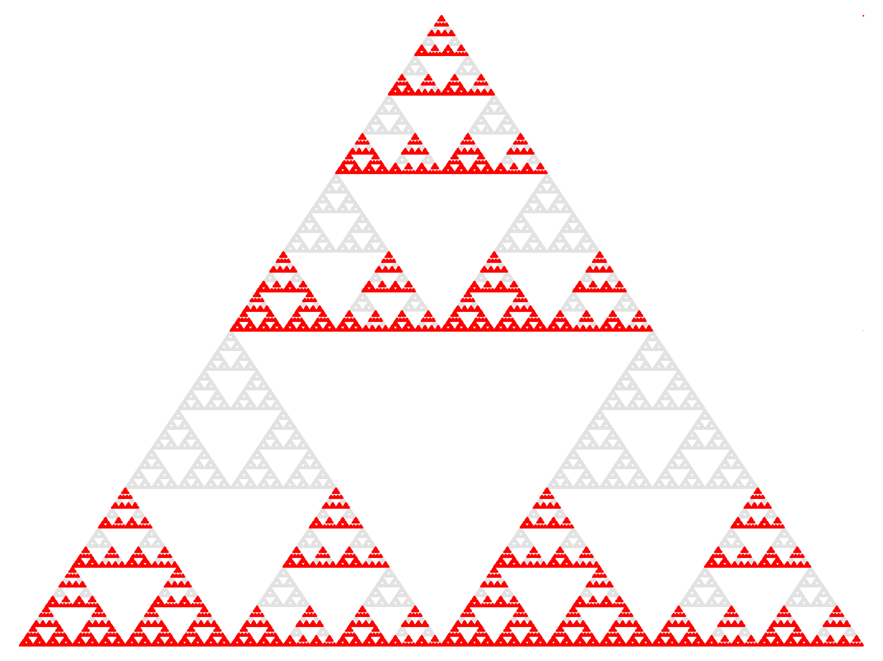
Figure 6: An asymmetrical regular subfractal of the Sierpinski Gasket generated by the process term $e=\mu v\leavevmode\nobreak\ (av+bg+cg)$, where $g=\mu u\leavevmode\nobreak\ (bu+bv+cv)$, corresponding to the same contraction operator interpretation as in Figure 2.

For another example involving the Sierpinski Gasket, see Figure 6. Let $g=\mu u\leavevmode\nobreak\ (bu+bv+cv)$, and note that $v$ is free in $g$. The asymmetrical regular subfractal appearing in Figure 6 is the regular subfractal semantics of the term $e=\mu v\leavevmode\nobreak\ (av+bg+cg)$ corresponding to the same contraction operator interpretation as in Figures 1 and 2.

$\begin{gathered}\leavevmode\hbox to116.63pt{\vbox to38.84pt{\text{[drawing]}}}\\ \begin{aligned} e&=\mu v\leavevmode\nobreak\ (av+bg+cg)\\ g&=\mu u\leavevmode\nobreak\ (bu+bv+cv)\\ f&=g[e/v]=\mu u\leavevmode\nobreak\ (bu+be+ce)\end{aligned}\end{gathered}$

Systems and Solutions

Self-similar sets are often characterized as the unique nonempty compact sets that solve systems of equations of the form

$$K=\sigma_{1}(K)\cup\cdots\cup\sigma_{n}(K)$$

with each $\sigma_{i}$ a contraction operator on a complete metric space. For example, the Sierpiński gasket is the unique nonempty compact solution to $K=\sigma_{a}(K)\cup\sigma_{b}(K)\cup\sigma_{c}(K)$ in Figure 1. In this section, we are going to provide a similar characterization for regular subfractals that will play an important role in the completeness proof in Section 4. The main connection of the characterization above to trace semantics arises from thinking about an $n$-state LTS $(X,\alpha)$ as a system of formal equations for the trace sets associated to the states:

$$x_{i}=a_{i1}x_{i1}+a_{i2}x_{i2}+\cdots+a_{im_{i}}x_{im_{i}}$$

indexed by $X=\{x_{1},\dots,x_{n}\}$, where $x_{i}\mathrel{\raisebox{-1.0pt}{$\xrightarrow{a_{ij}}$}}_{\alpha}x_{ij}$ for $i\leq n$ and $j\leq m_{i}$.

Definition 27.

Given a contraction operator interpretation $\sigma:A\to\operatorname{Con}(M)$, and an LTS $(X,\alpha)$, we call a function $\varphi:X\to\mathbf{K}(M)$ a ($\sigma$-)solution to $(X,\alpha)$ if for any $x\in X$,

$$\varphi(x)=\bigcup_{x\mathrel{\raisebox{-1.0pt}{$\xrightarrow{a}$}}y}\sigma_{a}(\varphi(y))$$

Example 3.4.

Let $\mathbf{S}$ be the Sierpiński gasket as a subset of $\mathbb{R}^{2}$. Let $(X,\alpha)$ be the LTS in Figure 1. Then we have a single state, $x$, with $x\mathrel{\raisebox{-1.0pt}{$\xrightarrow{a,b,c}$}}x$. The function $\varphi\colon X\to\mathbf{K}(\mathbb{R}^{2})$ given by $\varphi(s)=\mathbf{S}$ is a solution to $(X,\alpha)$, because $\mathbf{S}=\sigma_{a}(\mathbf{S})\cup\sigma_{b}(\mathbf{S})\cup\sigma_{c}(\mathbf{S})$. Self-similar sets, in the sense of Hutchinson [16], are regular subfractals generated by one-state LTSs.

The following result, which is essentialy [24, Theorem 1], states that finite productive LTSs have unique solutions.

Lemma 3.5.

Let $M$ be a complete metric space, $\sigma:A\to\operatorname{Con}(M)$, and $(X,\alpha)$ be a finite productive LTS. Then $(X,\alpha)$ has a unique solution $\varphi_{\alpha}$.

The proof of Lemma 3.5 makes use of the Hausdorff metric on $\mathbf{K}(M)$, defined

$$d_{H}(K_{1},K_{2})=\max\left\{\sup_{u\in K_{1}}\inf_{v\in K_{2}}d(u,v),\sup_{v\in K_{2}}\inf_{u\in K_{1}}d(u,v)\right\}$$ (8)

This equips $\mathbf{K}(M)$ with the structure of a metric space. If $M$ is complete, so is $\mathbf{K}(M)$. Incidentally, we need to restrict to nonempty sets in (8), since otherwise we would worry about infima over the empty set. This is the primary motivation for the guardedness condition which we imposed on our terms. We also recall the Banach fixed-point theorem, which allows for the computation of fixed-points by iteration.

Theorem 3.6 (Banach [3]).

Let $M$ be a nonempty metric space and let $f\colon M\to M$ be a contraction map. Then the following two statements are true.

1. The map $f$ has at most one fixed-point. That is, if $p=f(p)$ and $q=f(q)$, then $p=q$.

2. If $M$ is complete, then for any $p\in M$, $\lim_{n\to\infty}f^{n}(p)$ is the unique fixed-point of $f$.

Fix a complete nonempty metric space $M$, a productive finite LTS $(X,\alpha)$, and a contraction operator interpretation $\sigma:A\to\operatorname{Con}(M)$. To compute the solution to $(X,\alpha)$, we iteratively apply a matrix-like operator to the set $\mathbf{K}(M)^{X}$ of vectors $[K_{x_{1}},\dots,K_{x_{n}}]$ with entries in $\mathbf{K}(M)$ indexed by $X$. Formally, we define

$${\left[\alpha\right]_{\sigma}}\colon\mathbf{K}(M)^{X}\to\mathbf{K}(M)^{X}\qquad({\left[\alpha\right]_{\sigma}}\vec{K})_{x}=\bigcup_{x\mathrel{\raisebox{-1.0pt}{$\xrightarrow{a}$}}y}\sigma_{a}(K_{y})$$

for each $x\in X$. Intuitively, ${\left[\alpha\right]_{\sigma}}$ acts like an $X\times X$-matrix of unions of contractions.

Proof 3.7 (Proof of Lemma 3.5.).

Every fixed-point of ${\left[\alpha\right]_{\sigma}}$ corresponds to a solution of $(X,\alpha)$. Indeed, given $\vec{F}$ such that ${\left[\alpha\right]_{\sigma}}\vec{F}=\vec{F}$, and defining $\varphi\colon X\to\mathbf{K}(M)$ by $\varphi(x)=F_{x}$, we see that

$$\varphi(x)=F_{x}=({\left[\alpha\right]_{\sigma}}\vec{F})_{x}=\bigcup_{x\mathrel{\raisebox{-1.0pt}{$\xrightarrow{a}$}}y}\sigma_{a}(F_{y})=\bigcup_{x\mathrel{\raisebox{-1.0pt}{$\xrightarrow{a}$}}y}\sigma_{a}(\varphi(y))$$

Conversely, if $\varphi:X\to\mathbf{K}(M)$ is a solution to $(X,\alpha)$, then defining $F_{x}=\varphi(x)$ we have

$$F_{x}=\varphi(x)=\bigcup_{x\mathrel{\raisebox{-1.0pt}{$\xrightarrow{a}$}}y}\sigma_{a}(\varphi(y))=\bigcup_{x\mathrel{\raisebox{-1.0pt}{$\xrightarrow{a}$}}y}\sigma_{a}(F_{y})=({\left[\alpha\right]_{\sigma}}\vec{F})_{x}$$

for each $x\in X$. Thus, it suffices to show that ${\left[\alpha\right]_{\sigma}}$ has a unique fixed-point. By the Banach Fixed-Point Theorem 3.6, we just need to show that ${\left[\alpha\right]_{\sigma}}$ is a contraction operator. That is, ${\left[\alpha\right]_{\sigma}}\in\operatorname{Con}(\mathbf{K}(M)^{X},d^{X})$, where $d^{X}$ is the product metric given in terms of the Hausdorff metric $d_{H}$, as follows:

$$d^{X}([K_{x_{1}},\ldots,K_{x_{n}}],[K^{\prime}_{x_{1}},\ldots,K^{\prime}_{x_{n}}])=\max\{d_{H}(K_{x_{i}},K^{\prime}_{x_{i}})\mid 1\leq i\leq n\}$$

This point is standard in the fractals literature; cf. [16].

Fractal Semantics and Solutions

Recall that the fractal semantics of a process term $e$ with respect to a contraction operator interpretation $\sigma\colon A\to\operatorname{Con}(M)$ is the set $\left\llbracket{e}\right\rrbracket_{\sigma}$ of limits of streams applied to points in the complete metric space $M$.

Theorem 3.8.

Let $(X,\alpha)$ be a finite productive LTS and let $x\in X$. Given $e\in\mathsf{Term}$, a complete metric space $M$, and $\sigma\colon A\to\operatorname{Con}(M)$. Then the following two statements are true.

1. $\left\llbracket{x}\right\rrbracket_{\alpha,\sigma}\in\mathbf{K}(M)$, i.e., $\left\llbracket{x}\right\rrbracket_{\alpha,\sigma}$ is nonempty and compact.

2. $\left\llbracket{-}\right\rrbracket_{\alpha,\sigma}\colon X\to\mathbf{K}(M)$ is the unique solution to $(X,\alpha)$.

In particular, $(\mathsf{Term},\gamma)$ is locally finite, and so by Lemma 3.5 has a unique solution. Theorem 3.8 therefore implies that this solution is $\left\llbracket{-}\right\rrbracket_{\sigma}$. We obtain the following, which can be seen as an analogue of Kleene’s theorem for regular expressions [18], as a direct consequence of Theorem 3.8.

Theorem 3.9.

A subset of a self-similar set is a regular subfractal if and only if it is a component of a solution to a finite productive LTS.

4 Fractal Equivalence is Traced

We have seen that finite productive LTSs (LTSs that only emit infinite streams) can be specified by process terms. We also introduced a family of fractal sets called regular subfractals, those subsets of self-similar sets obtained from the streams emitted by finite productive LTSs. An LTS itself is representative of a certain system of equations, and set-wise the system of equations is solved by the regular subfractals corresponding to it. Going from process terms to LTSs to regular subfractals, we see that a process term is representative of a sort of uninterpreted fractal recipe, which tells us how to obtain a regular subfractal from an interpretation of action symbols as contractions on a complete metric space.

Definition 4.1.

Let $(X,\alpha)$ be a productive LTS. Given $x,y\in X$, we write $x\approx y$ and say that $x$ and $y$ are fractal equivalent (or that they are equivalent fractal recipes) if $\left\llbracket{x}\right\rrbracket_{\alpha,\sigma}=\left\llbracket{y}\right\rrbracket_{\alpha,\sigma}$ for every complete metric space $M$ and every $\sigma:A\to\operatorname{Con}(M)$.

Theorem 4.2.

Let $(X,\alpha)$ be a finitely branching productive LTS and $x,y\in X$. Then $x\approx y$ if and only if $\operatorname{str}(x)=\operatorname{str}(y)$.

Proof 4.3.

Clearly, if $\operatorname{str}_{\alpha}(x)=\operatorname{str}_{\alpha}(y)$, then $x\approx y$ by definition. Conversely, consider the space $(A^{\omega},d)$ of streams from $A$ equipped with the $1/2$-metric below:

$$d((a_{1},\dots),(b_{1},\dots))=\inf\left\{2^{-n}\leavevmode\nobreak\ \middle|\leavevmode\nobreak\ (\forall i\leq n)\leavevmode\nobreak\ a_{i}=b_{i}\right\}$$ (9)

This space is the Cantor set on $|A|$ symbols, a compact metric space. We show that for any $x\in X$, $\operatorname{str}_{\alpha}(x)$ is a nonempty closed subset of $(A^{\omega},d)$, as follows.

Since $(X,\alpha)$ is finitely branching and productive, there is at least one infinite path beginning at $x$. This tells us that $\operatorname{str}_{\alpha}(x)\neq\emptyset$.

To see that $\operatorname{str}_{\alpha}(x)$ is closed, consider a Cauchy sequence $\{(a_{1}^{(i)},a_{2}^{(i)}\dots)\}_{i\in\mathbb{N}}$ in $\operatorname{str}_{\alpha}(x)$, and let $(a_{1},\dots)$ be its limit in $(A^{\omega},d)$. Then $x$ emits every finite initial segment of $(a_{1},\dots)$, because for any $N\in\mathbb{N}$, there is an $m\in\mathbb{N}$ such that $(a_{1},\dots,a_{m},a_{m+1}^{(m)},\dots)\in\operatorname{str}(x)$ for $m>N$. Since $(X,\alpha)$ is finitely branching and productive, Lemma 2.2 tells us that $(a_{1},\dots)\in\operatorname{str}_{\alpha}(x)$. Thus, $\operatorname{str}(x)$ is a non-empty closed set. By compactness of $(A^{\omega},d)$, we therefore have $\operatorname{str}(x)\in\mathbf{K}(A^{\omega})$, so $\operatorname{str}\colon X\to\mathbf{K}(A^{\omega})$.

For each $a\in A$, let $a(-):A^{\omega}\to A^{\omega}$ be the prefixing map $a(a_{1},\dots)=(a,a_{1},\dots)$. Then $a(-)$ has a contraction coefficient of $1/2$, and $\sigma(a)=a(-)$ defines a contraction operator interpretation $\sigma:A\to\operatorname{Con}(A^{\omega},d)$. By construction, $\operatorname{str}(x)=\bigcup_{x\mathrel{\raisebox{-1.0pt}{$\xrightarrow{a}$}}y}a(\operatorname{str}(y))$ for any $x\in X$. By the uniqueness of fixed points we saw in Lemma 3.5, we therefore have $\operatorname{str}(x)=\left\llbracket{x}\right\rrbracket_{\alpha,\sigma}$. Hence, if $x\approx y$, then $\operatorname{str}(x)=\left\llbracket{x}\right\rrbracket_{\alpha,\sigma}=\left\llbracket{y}\right\rrbracket_{\alpha,\sigma}=\operatorname{str}_{\alpha}(y)$.

This gives way to a soundness/completeness theorem for our version of Rabinovich’s logic with respect to its fractal semantics. Our proof relies on the logical characterization of trace equivalence that we saw in Theorem 2.10.

Theorem 4.4 (Soundness/Completeness).

Let $e,f\in\mathsf{Term}$. Then

$$e\approx f\leavevmode\nobreak\ \text{ if and only if }\leavevmode\nobreak\ e\equiv f$$

Proof 4.5.

Let $e,f\in\mathsf{Term}$. Then since $(\mathsf{Term},\gamma)$ is finitely branching and productive,

$$e\approx f\stackrel{{\scriptstyle\text{(\lx@cref{creftype~refnum}{thm:fractal equivalence is traced})}}}{{\iff}}\operatorname{str}(e)=\operatorname{str}(f)\stackrel{{\scriptstyle\text{(\lx@cref{creftype~refnum}{lem:trace stream equivalence})}}}{{\iff}}\operatorname{tr}(e)=\operatorname{tr}(f)\stackrel{{\scriptstyle\text{(\lx@cref{creftype~refnum}{thm:Rabinovich})}}}{{\iff}}e\equiv f$$

5 A Calculus of Subfractal Measures

Aside from showing the existence of self-similar sets and their correspondence with contraction operator interpretations (in Hutchinson’s terminology, iterated function systems), Hutchinson also shows that every probability distribution on the contractions corresponds to a unique measure, called the invariant measure, that satisfies a certain recursive equation and whose support is the self-similar set. In this section, we replay the story up to this point, but with Hutchinson’s invariant measure construction instead of the invariant (self-similar) set construction. We specify fractal measures using a probabilistic version of LTSs called labelled Markov chains, as well as a probabilistic version of Milner’s specification language introduced by Stark and Smolka [35]. Similar to how fractal equivalence coincides with trace equivalence, fractal measure equivalence is equivalent to a probabilistic version of trace equivalence due to Kerstan and König [17].

Invariant measures

Recall that a Borel probability measure on a metric space $M$ is a $[0,\infty]$-valued function $\rho$ defined on the Borel subsets of $M$ (the smallest $\sigma$-algebra containing the open balls of $M$) that is countably additive and assigns $\rho(\emptyset)=0$ and $\rho(M)=1$. A Borel probability measure $\rho$ is supported by a point $p\in M$ if for any open set $U$ containing $p$, $\rho(U)>0$. A Borel probability measure is compactly supported if the set of points supporting it is a compact set. Note that the support of a Borel measure is always a closed set, so a Borel measure is compactly supported if and only if its support is bounded. For a more detailed introduction to Borel measures, see for example [13].

Hutchinson shows in [16] that, given $\sigma\colon A\to\operatorname{Con}(M)$, each probability distribution $\theta\colon A\to[0,1]$ on $A$ gives rise to a unique compactly supported Borel probability measure $\hat{\theta}_{\sigma}$ on $M$, called the invariant measure, that is supported by the self-similar set $\mathbf{S}_{\sigma}$ from (5) and such that for any Borel set $B\subseteq M$,

$$\hat{\theta}_{\sigma}(B)=\sum_{a\in A}\theta(a)\leavevmode\nobreak\ \sigma_{a}^{\#}\hat{\theta}_{\sigma}(B)$$ (10)

Here and elsewhere, the pushforward $f^{\#}\rho$ of a Borel measure $\rho$ with respect to a continuous (or more generally, Borel measurable) map $f$ is the probability measure defined by $f^{\#}\rho(B)=\rho(f^{-1}(B))$ for any Borel subset $B$ of $M$ [13]. The pushforwards $\sigma_{a}^{\#}\hat{\theta}_{\sigma}$ in (10) are well-defined because contractions are continuous maps. Equation 10 tells us that, similar to how self-similar sets are the union of their images over a set of contractions, the invariant measure $\hat{\theta}_{\sigma}$ is a sum of its pushforwards with respect to a set of contractions.

We can use the first part of the Banach Fixed Point Theorem, Theorem 3.6 (1), to show that (10) is satisfied by at most one compactly supported Borel measure on $M$. Indeed, fix a complete metric space $M$.

Definition 5.1.

We write $\mbox{\sf Prob}(M)$ for the set of compactly supported Borel probability measures on $M$ equipped with the Kantorovich-Rubinstein metric, defined by

$$d(\rho_{1},\rho_{2})=\sup\Big{\{}\int f\leavevmode\nobreak\ d\rho_{1}-\int f\leavevmode\nobreak\ d\rho_{2}\leavevmode\nobreak\ \Big{|}\leavevmode\nobreak\ f\colon M\to\mathbb{R}\text{ is nonexpanding}\Big{\}}$$

for any $\rho_{1},\rho_{2}\in\mbox{\sf Prob}(M)$. Above, $\int f\leavevmode\nobreak\ d\rho_{i}$ is given by the Lebesgue integral.

It is important to note that finiteness of $d(\rho_{1},\rho_{2})$ requires the assumption that $\rho_{1}$ and $\rho_{2}$ are compactly supported (equivalently, have bounded support).

Given a fixed probability distribution $\theta\colon A\to[0,1]$, we can rephrase (10) as a fixed-point equation for the Markov operator $F\colon\mbox{\sf Prob}(M)\to\mbox{\sf Prob}(M)$, defined by

$$F(\mu)=\sum_{a\in A}\theta(a)\leavevmode\nobreak\ \sigma_{a}^{\#}\mu$$ (11)

for each $\mu\in\mbox{\sf Prob}(M)$. Hutchinson proves in [16, 4.4 (1) Theorem] that $F$ is a contraction in the Kantorovich-Rubinstein metric. Therefore, if $F$ has a fixed-point, then Theorem 3.6 (1) tells us it is unique, and we can take the invariant measure to be this unique fixed-point of $F$.

However, it is not true for an arbitrary complete metric space $M$ that $\mbox{\sf Prob}(M)$ is complete, so we cannot apply Theorem 3.6 (2) to prove the existence of the invariant measure. In the next two paragraphs, we describe an explicit construction of the invariant measure. A more general construction and verification of its stated properties can be found in Theorem 5.9.

The invariant measure can be concretely described as follows. Given $\sigma\colon A\to\operatorname{Con}(M)$, let $c_{a}>0$ be a contraction coefficient for $\sigma_{a}$ for each $a\in A$. Define $(A^{\omega},d_{\sigma})$ to be the space of streams from $A$ equipped with the metric $d_{\sigma}$, given by

$$d_{\sigma}((a_{1},a_{2},\dots),(b_{1},b_{2},\dots))=\begin{cases}0&\text{if }a_{n}=b_{n}\text{ for all }n\\ \prod_{i=1}^{n}c_{a_{i}}&n=\min\{n\mid a_{n+1}\neq b_{n+1}\}\text{, otherwise}\end{cases}$$ (12)

Then $(A^{\omega},d_{\sigma})$, called the symbolic space associated with $\sigma$, is a compact metric space (it is homeomorphic to the Cantor set on $|A|$ symbols from the proof of Theorem 4.2) and has a basis of open sets given by

$$B_{w}=\{(a_{1},\dots,a_{n},b_{1}\dots)\mid(b_{1},\dots)\in A^{\omega}\}$$

for each $w=a_{1}\dots a_{n}$ in $A^{*}$. Note that $B_{\epsilon}=A^{\omega}$. Now, given a probability distribution $\theta\colon A\to[0,1]$, we define $\hat{\theta}$, the stream measure specified by $\theta$, to be the unique Borel probability distribution on $(A^{\omega},d_{\sigma})$ such that

$$\hat{\theta}(B_{w})=\prod_{i=1}^{n}\theta(a_{i})$$ (13)

for any $w=a_{1}\cdots a_{n}\in A^{*}$ (here, we take the empty product to be $1$). As will be explained shortly, results from [17] tell us that (13) does indeed extend to a unique Borel probability measure on $(A^{\omega},d_{\sigma})$. In particular, any two Borel measures that agree on all basic open sets must agree on all Borel sets. The next proposition tells us that the invariant measure is precisely $\hat{\theta}_{\sigma}=\sigma_{\omega}^{\#}\hat{\theta}$, where $\sigma_{\omega}$ is the map given by limits from 25.

Proposition 5.2.

Let $M$ be a complete metric space, let $\sigma\colon A\to\operatorname{Con}(M)$, and let $F$ be the Markov operator defined in (11). The pushforward $\sigma_{\omega}^{\#}\hat{\theta}$ of the measure $\hat{\theta}$ defined in (13) is the unique fixed-point of $F$, where $\sigma_{\omega}$ is defined as in 25.

Proof 5.3.

Given $\sigma\colon A\to\operatorname{Con}(M)$, let $\rho=\sigma_{\omega}^{\#}\hat{\theta}$. To see that $\rho$ is a fixed-point of the Markov operator $F$, i.e., $\rho$ satisfies (10), we observe that for any Borel set $B$,

$$\rho(B)=\sigma_{\omega}^{\#}\hat{\theta}(B) =\hat{\theta}(\sigma_{\omega}^{-1}(B))$$

$$=\hat{\theta}\Big{(}\bigcup_{a\in A}a(a^{-1}\circ\sigma_{\omega}^{-1}(B))\Big{)} \sigma_{\omega}^{-1}(B)$$ ( a stream language)

$$=\sum_{a\in A}\hat{\theta}(a(a^{-1}\circ\sigma_{\omega}^{-1}(B))) \hat{\theta} \bigcup_{a\in A}a(-)$$ ( a measure, a disjoint union)

$$=\sum_{a\in A}\theta(a)\leavevmode\nobreak\ \hat{\theta}((\sigma_{\omega}\circ a(-))^{-1}(B)) a^{-1}\circ\sigma_{\omega}^{-1}=(\sigma_{\omega}\circ a(-))^{-1}$$ (13), ()

$$=\sum_{a\in A}\theta(a)\leavevmode\nobreak\ \hat{\theta}((\sigma_{a}\circ\sigma_{\omega})^{-1}(B))$$ (6)

$$=\sum_{a\in A}\theta(a)\leavevmode\nobreak\ \sigma_{a}^{\#}\sigma_{\omega}^{\#}\hat{\theta}(B) (\sigma_{a}\circ\sigma_{\omega})^{-1}=\sigma_{\omega}^{-1}\circ\sigma_{a}^{-1}$$ ()

$$=\sum_{a\in A}\theta(a)\leavevmode\nobreak\ \sigma_{a}^{\#}\rho(B) \rho$$ (def. of )

Hence, $\rho$ is a fixed-point of $F$. We have already argued that $F$ has at most one fixed-point, so $\rho$ is the unique fixed-point of $F$. In other words, the invariant measure $\hat{\theta}_{\sigma}$ is precisely the pushforward measure $\sigma_{\omega}^{\#}\hat{\theta}$.

In the sequel, we are going to view the specification $\theta$ of the invariant measure $\hat{\theta}_{\sigma}$ (the pushforward of the stream measure) as a probability distribution over the transitions in a one-state LTS. This construction generalizes to multiple-state transition systems by moving from probability distributions on $A$ to labelled Markov chains, which are essentially LTSs where each state comes equipped with a probability distribution on its outgoing transitions. Again, the labels will be interpreted as contractions on a complete metric space.

Labelled Markov Chains

Let ${\mathcal{D}}$ denote the finitely supported probability distribution functor on the category of sets. LMCs generalize our specification of invariant measures with arbitrary finitely branching LTSs by replacing finite sets with finitely supported probability distributions.

Definition 5.4.

A labelled Markov chain (LMC) is a pair $(X,\beta)$ consisting of a set $X$ of states and a transition function $\beta\colon X\to{\mathcal{D}}(A\times X)$. A homomorphism of LMCs $h\colon(X,\beta_{X})\to(Y,\beta_{Y})$ is a map $h\colon X\to Y$ such that

$${\mathcal{D}}(1_{A}\times h)\circ\beta_{X}=\beta_{Y}\circ h$$

where $1_{A}$ is the identity map on $A$ and ${\mathcal{D}}(f)(\theta)(y)=\sum_{f(x)=y}\theta(x)$ for any $f\colon X\to Y$. We write $x\mathrel{\raisebox{-1.0pt}{$\xrightarrow{r\mid a}$}}_{\beta}y$ if $\beta(x)(a,y)=r$, often dropping the symbol $\beta$ if it is clear form context.

As we have already seen, given a complete metric space $M$ and a contraction operator interpretation $\sigma\colon A\to\operatorname{Con}(M)$, every state $x$ of a productive LTS $(X,\alpha)$ with labels in $A$ corresponds to a regular subfractal $\left\llbracket{x}\right\rrbracket_{\alpha,\sigma}$ of the set $\mathbf{S}_{\sigma}$ from Definition 5. This regular subfractal is the continuous image of the set $\operatorname{str}(x)$ under the map $\sigma_{\omega}\colon(A^{\omega},d_{\sigma})\to M$. The family $\left\llbracket{x}\right\rrbracket_{\alpha,\sigma}$ is characterized by its satisfaction of the equations representing the LTS $(X,\alpha)$.

Every LMC $(X,\beta)$ has an underlying LTS $(X,\bar{\beta})$, where $\bar{\beta}(x)=\{(a,y)\mid\beta(x)(a,y)>0\}$. Note that since $\beta(x)$ is a probability distribution, our underlying LTS is automatically productive since at least one transition must have positive probability. For each $x\in X$, we are going to define a probability measure $\hat{\beta}_{\sigma}(x)$ on $\mathbf{S}_{\sigma}$ whose support is $\left\llbracket{x}\right\rrbracket_{\bar{\beta},\sigma}$, and that satisfies a recursive system of equations represented by the LMC $(X,\beta)$. Roughly, $\hat{\beta}_{\sigma}(x)$ is the pushforward of a certain Borel probability measure $\hat{\beta}(x)$ on $A^{\omega}$.

Again, we topologize $A^{\omega}$, using as a basis the sets of the form

$$B_{w}=\{(a_{1},\dots,a_{n},b_{1},\dots)\mid(b_{1},\dots)\in A^{\omega}\}$$

where $w=a_{1}\cdots a_{n}\in A^{*}$. Given a state $x$ of a LMC $(X,\beta)$ and a word $w=a_{1}\cdots a_{n}$, we follow Kerstan and König [17] and define the trace measure of the basic open set $B_{w}$ by

$$\hat{\beta}(x)(B_{w})=\sum\{r_{1}\cdots r_{n}\mid x\mathrel{\raisebox{-1.0pt}{$\xrightarrow{r_{1}\mid a_{1}}$}}x_{1}\mathrel{\raisebox{-1.0pt}{$\xrightarrow{\phantom{\ \mid\ }}$}}\cdots\mathrel{\raisebox{-1.0pt}{$\xrightarrow{r_{n}\mid a_{n}}$}}x_{n}\}$$ (14)

where $\hat{\beta}(x)(B_{\epsilon})=\hat{\beta}(x)(A^{\omega})=1$. We provide the following convenient proposition, which tells us that (14) defines a unique Borel probability measure on $(A^{\omega},d)$.

Proposition 5.5.

Let $j\colon A^{*}\to[0,1]$ satisfy $j(w)=\sum_{a\in A}j(wa)$ for any $w\in A^{*}$ and $j(\epsilon)=1$, where $\epsilon$ is the empty word. Then there is a unique compactly supported Borel probability measure $\rho\in\mbox{\sf Prob}(A^{\omega})$ such that for any $w\in A^{*}$, $\rho(B_{w})=j(w)$.

The following proof is a simple stitching together of results from [17].

Proof 5.6.

Let $\mathcal{S}_{\omega}=\{\emptyset\}\cup\{B_{w}\mid w\in A^{*}\}$, and define $\rho_{0}\colon\mathcal{S}_{\omega}\to[0,1]$ by $\rho_{0}(B_{w})=j(w)$ and $\rho_{0}(\emptyset)=0$. We know from [17, Lemma 3.17] that there exists a Borel measure $\rho$ on $A^{\omega}$ such that $\rho(B_{w})=\rho_{0}(B_{w})$ for every $w\in A^{*}$. By [17, Proposition 3.5], $\mathcal{S}_{\omega}$ is a covering semiring of sets, i.e., (i) $\emptyset\in\mathcal{S}_{\omega}$, (ii) $\mathcal{S}_{\omega}$ is closed under intersections, (iii) if $U,V\in\mathcal{S}_{\omega}$ then there exist $S_{1},\dots,S_{n}\in\mathcal{S}_{\omega}$ such that $U\setminus V=\bigcup_{i=1}^{n}S_{i}$, and (iv) there exist $S_{0},S_{1},\dots\in\mathcal{S}$ such that $A^{\omega}=\bigcup_{n\in\mathbb{N}}S_{n}$ (in fact, $A^{\omega}=B_{\epsilon}\in S_{\omega}$). Thus, there is exactly one Borel measure $\rho$ such that $\rho(B_{w})=\rho_{0}(B_{w})=j(w)$ for every $B_{w}\in\mathcal{S}_{\omega}$ by [17, Corollary 2.5]. Of course, $B_{\epsilon}=A^{\omega}$, so $\rho(B_{\epsilon})=1$ implies that $\rho$ is a probability measure. And finally, since $A^{\omega}$ is compact, all Borel measures on $A^{\omega}$ are compactly supported. Hence, $\rho\in\mbox{\sf Prob}(A^{\omega})$.

In particular, given any LMC $(X,\beta)$, $\hat{\beta}(x)(B_{w})=\sum_{a\in A}\hat{\beta}(x)(B_{wa})$, so there is a unique Borel probability measure $\hat{\beta}(x)$ on $A^{\omega}$ such that (14) holds for any basic open set $B_{w}$.

Definition 5.7.

Let $(X,\beta)$ be an LMC, and $\sigma\colon A\to\operatorname{Con}(M)$ be a contraction operator interpretation in a complete metric space. For each $x\in X$, we define the regular subfractal measure corresponding to $x$ to be $\hat{\beta}_{\sigma}(x)=\sigma_{\omega}^{\#}\hat{\beta}(x)$.

Intuitively, the regular subfractal measure of a state in a LMC under a contraction operator interpretation computes the probability that, if run stochastically according to the probabilities labelling the edges, the sequence of points of $M$ observed in the run eventually lands within a given Borel subset of $M$.

Systems of Probabilistic Equations

Fix a complete metric space $M$. In previous sections, we made use of the fact that, when $\sigma\colon A\to\operatorname{Con}(M)$, we can see $\mathbf{K}(M)$ as a semilattice with operators, i.e., union acts as a binary operation $\cup\colon\mathbf{K}(M)^{2}\to\mathbf{K}(M)$ and each $\sigma_{a}\colon\mathbf{K}(M)\to\mathbf{K}(M)$ distributes over $\cup$. Analogously, equipped with $\sigma\colon A\to\operatorname{Con}(M)$, $\mbox{\sf Prob}(M)$ is a convex algebra with operators. Formally, for any $r\in(0,1)$, there is a binary operation $\oplus_{r}\colon\mbox{\sf Prob}(M)^{2}\to\mbox{\sf Prob}(M)$ defined $(\rho_{1}\oplus_{r}\rho_{2})(B)=r\rho_{1}(B)+(1-r)\rho_{2}(B)$, over which each $\sigma_{a}^{\#}$ distributes, i.e.,

$$\sigma_{a}^{\#}(\rho_{1}\oplus_{r}\rho_{2})=\sigma_{a}^{\#}\rho_{1}\oplus_{r}\sigma_{a}^{\#}\rho_{2}$$

We also make use of a summation notation defined for any $r_{1},\dots,r_{n}\in[0,1)$ by

$$r_{1}\cdot\rho_{1}\oplus\cdots\oplus r_{n}\cdot\rho_{n}=\rho_{n}\oplus_{r_{n}}\left(\frac{r_{1}}{1-r_{n}}\cdot\rho_{1}\oplus\cdots\oplus\frac{r_{n-1}}{1-r_{n}}\cdot\rho_{n-1}\right)$$

Given a contraction operator interpretation, an LMC $(X,\beta)$ can be thought of as a system of equations in which one side is a polynomial term in a convex algebra with operators,

$$x_{i}=r_{i1}\cdot a_{i1}x_{i1}\oplus r_{i2}\cdot a_{i2}x_{i2}\oplus\cdots\oplus r_{im_{i}}\cdot a_{im_{i}}x_{im_{i}}$$

where $X=\{x_{1},\dots,x_{n}\}$ and $x_{i}\mathrel{\raisebox{-1.0pt}{$\xrightarrow{r_{ij}\mid a_{ij}}$}}x_{ij}$ for each $i\leq n$ and $j\leq m_{i}$.

Definition 5.8.

Let $(X,\beta)$ be a LMC, and let $\sigma\colon A\to\operatorname{Con}(M)$. A solution to $(X,\beta)$ is a function $\varphi\colon X\to\mbox{\sf Prob}(M)$ such that for any $x\in X$ and any Borel set $B\subseteq M$,

$$\varphi(x)(B)=\sum_{x\mathrel{\raisebox{-1.0pt}{$\xrightarrow{r\mid a}$}}y}r\leavevmode\nobreak\ \sigma_{a}^{\#}(\varphi(y))(B)$$

Every finite LMC admits a unique solution, and moreover, the unique solution is the regular subfractal measure from Definition 5.7.

Theorem 5.9.

Let $(X,\beta)$ be a LMC, $x\in X$, and $\sigma\colon A\to\operatorname{Con}(M)$. Then the map $\hat{\beta}_{\sigma}\colon X\to\mbox{\sf Prob}(M)$ is the unique solution to $(X,\beta)$.

Proof 5.10 (Proof.).

We are going to show (i) that the map $F_{\beta}\colon\mbox{\sf Prob}(M)^{X}\to\mbox{\sf Prob}(M)^{X}$ defined by

$$F_{\beta}(h)(x)(B)=\sum_{x\mathrel{\raisebox{-1.0pt}{$\xrightarrow{r\mid a}$}}y}r\leavevmode\nobreak\ \sigma_{a}^{\#}h(y)(B)$$

is a contraction mapping in the product metric on $(\mbox{\sf Prob}(M)^{X},d^{X})$, i.e., $d^{X}(h_{1},h_{2})=\max\{d(h_{1}(y),h_{2}(y))\mid y\in X\}$, and (ii) that $\hat{\beta}_{\sigma}$ is a fixed-point of this mapping.

For (i), we reuse the proof technique of [16, Theorem 4.4 (1)]. For each $a\in A$, let $c_{a}$ be a nonzero contraction coefficient for $\sigma_{a}$. Let $c=\max\{c_{a}\mid a\in A\}$, so that $0<c<1$ and for any $a\in A$, $c_{a}/c\leq 1$. For any nonexpanding $f\colon M\to\mathbb{R}$ and any $y\in X$,

$$\int_{M}f\leavevmode\nobreak\ d(\sigma_{a}^{\#}h(y))=c\int_{M}\frac{1}{c}f\leavevmode\nobreak\ d(\sigma_{a}^{\#}h(y))=c\int_{M}\frac{1}{c}f\circ\sigma_{a}\leavevmode\nobreak\ dh(y)$$

Since $0<c_{a}/c\leq 1$, $\frac{1}{c}f\circ\sigma_{a}$ is a nonexpanding map into $\mathbb{R}$. Where $d$ is the Kantorovich-Rubenstein metric, this implies that for any $\rho_{1},\rho_{2}\in\mbox{\sf Prob}(M)$,

$$\int_{M}\frac{1}{c}f\circ\sigma_{a}\leavevmode\nobreak\ d\rho_{1}-\int_{M}\frac{1}{c}f\circ\sigma_{a}\leavevmode\nobreak\ d\rho_{2}\leq d(\rho_{1},\rho_{2})$$ (15)

Putting these observations together, we obtain the following for any $h_{1},h_{2}\colon X\to\mbox{\sf Prob}(M)$. If $f\colon M\to\mathbb{R}$ is a nonexpanding map, then

$$\int_{M}f\leavevmode\nobreak\ dF_{\beta}(h_{1})(x)-\int_{M}f\leavevmode\nobreak\ dF_{\beta}(h_{2})(x)$$

$$=\int_{M}\sum_{x\mathrel{\raisebox{-1.0pt}{$\xrightarrow{r\mid a}$}}y}rf\leavevmode\nobreak\ d(\sigma_{a}^{\#}h_{1}(y))-\int_{M}\sum_{x\mathrel{\raisebox{-1.0pt}{$\xrightarrow{r\mid a}$}}y}rf\leavevmode\nobreak\ d(\sigma_{a}^{\#}h_{2}(y)) F$$ (definition of )

$$=\sum_{x\mathrel{\raisebox{-1.0pt}{$\xrightarrow{r\mid a}$}}y}r\Big{(}\int_{M}f\leavevmode\nobreak\ d(\sigma_{a}^{\#}h_{1}(y))-\int_{M}f\leavevmode\nobreak\ d(\sigma_{a}^{\#}h_{2}(y))\Big{)} \int$$ (linearity of )

$$=\sum_{x\mathrel{\raisebox{-1.0pt}{$\xrightarrow{r\mid a}$}}y}rc\Big{(}\int_{M}\frac{1}{c}f\circ\sigma_{a}\leavevmode\nobreak\ dh_{1}(y)-\int_{M}\frac{1}{c}f\circ\sigma_{a}\leavevmode\nobreak\ dh_{2}(y)\Big{)} \int$$ (linearity of )

$$\leq\sum_{x\mathrel{\raisebox{-1.0pt}{$\xrightarrow{r\mid a}$}}y}rc\leavevmode\nobreak\ d(h_{1}(y),h_{2}(y))$$ (15)

$$\leq c\leavevmode\nobreak\ \max\{d(h_{1}(y),h_{2}(y))\mid y\in X,x\mathrel{\raisebox{-1.0pt}{$\xrightarrow{r\mid a}$}}y\} \sum r=1$$ ()

$$\leq c\leavevmode\nobreak\ d^{X}(h_{1},h_{2}) d^{X}$$ (def. of )

Since $d^{X}(F(h_{1}),F(h_{2}))=\max\{d(F(h_{1})(x),F(h_{2})(x))\mid x\in X\}$ and $d(F(h_{1})(x),F(h_{2})(x))$ is the supremum over nonexpanding $f\colon M\to\mathbb{R}$ in the first expression in the calculation above, this shows that $F_{\beta}$ is a contraction mapping in the product metric on $\mbox{\sf Prob}(M)^{X}$.

To see item (ii), we begin by showing that for any $x\in X$ and Borel set $B\subseteq A^{\omega}$,

$$\hat{\beta}(x)(B)=\sum_{x\mathrel{\raisebox{-1.0pt}{$\xrightarrow{r\mid a}$}}y}r\leavevmode\nobreak\ \sigma_{a}^{\#}\beta(x)(B)$$ (16)

By the Identity and Extension Theorems for $\sigma$-finite premeasures [17], it suffices to show (16) for each basic open set $B=B_{w}$, with $w\in A^{*}$. We proceed with a case analysis on $w$. In the first case, $w=\epsilon$. Let $a(-)$ be the prefixing map $a(a_{1},\dots)=(a,a_{1},\dots)$ on $A^{\omega}$. Since $a^{-1}(A^{\omega})=A^{\omega}$ and $\sum\{r\mid x\mathrel{\raisebox{-1.0pt}{$\xrightarrow{r\mid a}$}}y\}=1$,

$$\hat{\beta}(x)(B_{\epsilon})=\hat{\beta}(x)(A^{\omega})=1=\sum_{x\mathrel{\raisebox{-1.0pt}{$\xrightarrow{r\mid a}$}}y}r\leavevmode\nobreak\ \hat{\beta}(y)(a^{-1}(A^{\omega}))=\sum_{x\mathrel{\raisebox{-1.0pt}{$\xrightarrow{r\mid a}$}}y}r\leavevmode\nobreak\ a^{\#}\hat{\beta}(y)(B_{\epsilon})$$

In the second case, $w$ is nonempty. Let $a\in A$ and $w=a_{1}\cdots a_{n}$. Then

$$\hat{\beta}(x)(B_{aw}) =\sum\{rr_{1}\cdots r_{n}\mid x\mathrel{\raisebox{-1.0pt}{$\xrightarrow{r\mid a}$}}y\mathrel{\raisebox{-1.0pt}{$\xrightarrow{r_{1}\mid a_{1}}$}}y_{1}\mathrel{\raisebox{-1.0pt}{$\xrightarrow{\phantom{r\mid a}}$}}\cdots\mathrel{\raisebox{-1.0pt}{$\xrightarrow{\phantom{r\mid a}}$}}x_{n}\}$$

$$=\sum_{x\mathrel{\raisebox{-1.0pt}{$\xrightarrow{r\mid a}$}}y}r\leavevmode\nobreak\ \sum\{r_{1}\cdots r_{n}\mid y\mathrel{\raisebox{-1.0pt}{$\xrightarrow{r_{1}\mid a_{1}}$}}y_{1}\mathrel{\raisebox{-1.0pt}{$\xrightarrow{\phantom{r\mid a}}$}}\cdots\mathrel{\raisebox{-1.0pt}{$\xrightarrow{\phantom{r\mid a}}$}}x_{n}\}$$

$$=\sum_{x\mathrel{\raisebox{-1.0pt}{$\xrightarrow{r\mid a}$}}y}r\leavevmode\nobreak\ \hat{\beta}(y)(B_{w})$$

$$=\sum_{x\mathrel{\raisebox{-1.0pt}{$\xrightarrow{r\mid a}$}}y}r\leavevmode\nobreak\ \hat{\beta}(y)(a^{-1}(B_{aw})) a^{-1}(B_{aw})=B_{w}$$ ()

$$=\sum_{x\mathrel{\raisebox{-1.0pt}{$\xrightarrow{r\mid a}$}}y}r\leavevmode\nobreak\ a^{\#}\hat{\beta}(y)(B_{aw})$$

Thus, for any Borel set $B\subseteq A^{\omega}$,

$$\hat{\beta}(x)(B)=\sum_{x\mathrel{\raisebox{-1.0pt}{$\xrightarrow{r\mid a}$}}y}r\leavevmode\nobreak\ a^{\#}\hat{\beta}(y)(B).$$ (17)

Finally, we will use Equation 17 to prove (ii). For any $x\in X$ and Borel set $B\subseteq M$,

$$\hat{\beta}_{\sigma}(x)(B) =\sigma_{\omega}^{\#}\hat{\beta}(x)(B)$$

$$=\hat{\beta}(x)(\sigma_{\omega}^{-1}(B))$$

$$=\sum_{x\mathrel{\raisebox{-1.0pt}{$\xrightarrow{r\mid a}$}}y}r\leavevmode\nobreak\ a^{\#}\hat{\beta}(y)(\sigma_{\omega}^{-1}(B))$$ (17)

$$=\sum_{x\mathrel{\raisebox{-1.0pt}{$\xrightarrow{r\mid a}$}}y}r\hat{\beta}(y)((\sigma_{\omega}\circ a(-))^{-1}(B)) a^{-1}\circ\sigma_{\omega}^{-1}=(\sigma_{\omega}\circ a(-))^{-1}$$ ()

$$=\sum_{x\mathrel{\raisebox{-1.0pt}{$\xrightarrow{r\mid a}$}}y}r\leavevmode\nobreak\ \hat{\beta}(y)((\sigma_{a}\circ\sigma_{\omega})^{-1}(B))$$ (6)

$$=\sum_{x\mathrel{\raisebox{-1.0pt}{$\xrightarrow{r\mid a}$}}y}r\leavevmode\nobreak\ \sigma_{a}^{\#}\sigma_{\omega}^{\#}\hat{\beta}(y)(B) \sigma_{\omega}^{-1}\circ\sigma_{a}^{-1}=(\sigma_{a}\circ\sigma_{\omega})^{-1}$$ ()

$$=F_{\beta}(\hat{\beta}_{\sigma})(x)(B) F_{\beta},\hat{\beta}_{\sigma}$$ (def. of )

Furthermore, since the support of $\hat{\beta}(x)$ is precisely $\operatorname{str}(x)$, the support of $\hat{\beta}_{\sigma}(x)$ is precisely the compact set $\sigma_{\omega}(\operatorname{str}(x))$, which we have already seen is the regular subfractal determined by the state $x$ of the underlying LTS of $(X,\beta)$. Hence, $\hat{\beta}_{\sigma}$ is the unique solution to $(X,\beta)$.

Probabilistic Process Terms

Finally, we introduce a syntax for specifying LMCs. Our specification language is essentially the productive fragment of Stark and Smolka’s process calculus [35], meaning that the expressions do not involve deadlock and all variables are guarded (see Definition 1).

Definition 5.11.

The set of probabilistic terms is given by the grammar

$$v\mid ae\mid e_{1}\oplus_{r}e_{2}\mid\mu v\leavevmode\nobreak\ e$$

Here $r\in(0,1)$, and otherwise we make the same stipulations as in 1. The set of probabilistic process terms $\mathsf{PTerm}$ consists of the closed and guarded probabilistic terms.

Instead of languages of streams, the analog of trace semantics appropriate for probabilistic process terms is a measure-theoretic semantics consisting of trace measures introduced earlier in this section (Equation 14).

Definition 5.12.

We define the LMC $(\mathsf{PTerm},\delta)$ in Figure 7 and call it the syntactic LMC. The trace measure semantics $\operatorname{trm}(e)$ of a probabilistic process term $e$ is defined to be $\operatorname{trm}(e)=\hat{\delta}(e)$. Given $\sigma\colon A\to\operatorname{Con}(M)$, the subfractal measure semantics of $e\in\mathsf{PTerm}$ corresponding to $\sigma$ is $\hat{\delta}_{\sigma}(e)$.

$$\delta(ae)(b,f) =\begin{cases}1&f=e\text{ and }b=a\\ 0&\text{otherwise}\end{cases}$$

$$\delta(e_{1}\oplus_{r}e_{2})(b,f) =r\delta(e_{1})(b,f)+(1-r)\delta(e_{2})(b,f)$$

$$\delta(\mu v\leavevmode\nobreak\ e)(b,f) =\delta(e[\mu v\leavevmode\nobreak\ e/v])(b,f)$$

Figure 7: The LMC structure $(\mathsf{PTerm},\delta)$. Above, $a,b\in A$, $r\in(0,1)$, and $e,e_{i},f\in\mathsf{PTerm}$.

Intuitively, the trace measure semantics of a process term $e$ assigns a Borel set of streams $B$ the probability that $e$ eventually emits a word in $B$. The next result gives a recursive method for computing the trace measure semantics of a process term. This recursive method will be useful in Section 6.

Lemma 5.13.

For any $w\in A^{*}$, $a\in A$, $e,e_{i}\in\mathsf{PTerm}$, and $r\in(0,1)$, $\operatorname{trm}(e)(A^{\omega})=1$ and

$$\operatorname{trm}(ae)(B_{w}) =\begin{cases}\operatorname{trm}(e)(B_{u})&\text{$w=au$}\\ 0&\text{otherwise}\end{cases}$$

$$\operatorname{trm}(e_{1}\oplus_{r}e_{2})(B_{w}) =r\operatorname{trm}(e_{1})(B_{w})+(1-r)\operatorname{trm}(e_{2})(B_{w})$$

$$\operatorname{trm}(\mu v\leavevmode\nobreak\ e)(B_{w}) =\operatorname{trm}(e[\mu v\leavevmode\nobreak\ e/v])(B_{w})$$

Proof 5.14.

For each probabilistic process term $e$, define $j(e)\colon A^{*}\to[0,1]$ inductively by

$$j(ae)(w)=\begin{cases}j(e)(u)&\text{$w=au$}\\ 0&\text{otherwise}\end{cases}\qquad\begin{aligned} j(e_{1}\oplus_{r}e_{2})(w)&=r\leavevmode\nobreak\ j(e_{1})(w)+(1-r)\leavevmode\nobreak\ j(e_{2})(w)\\ j(\mu v\leavevmode\nobreak\ e)(w)&=j(e[\mu v\leavevmode\nobreak\ e/v])(w)\end{aligned}$$

We are going to show that $j(e)(w)=\hat{\delta}(e)(B_{w})$ for every $e\in\mathsf{PTerm}$, and since $\hat{\delta}(e)$ already satisfies $\hat{\delta}(e)(B_{w})=\sum_{a\in A}\hat{\delta}(e)(B_{wa})$ and $\hat{\delta}(e)(A^{\omega})=1$, we get $j(w)=\sum_{a\in A}j(wa)$ and $j(\epsilon)=1$, allowing us to apply the uniqueness part of Proposition 5.5. The proof is a multi-level induction:

1. The top level induction is by induction on words.

2. The second level induction is by induction on the unravelling number of probabilistic process terms, the smallest integer $\#_{un}(e)$ such that

   $$\#_{un}(ae)=0\qquad\#_{un}(e_{1}\oplus_{r}e_{2})=\max_{i\in\{1,2\}}\{\#_{un}(e_{i})\}\qquad\#_{un}(\mu v\leavevmode\nobreak\ e)=1+\#_{un}(e[\mu v\leavevmode\nobreak\ e/v])$$

3. The third level induction is on the number of probabilistic summands in a term with a fixed unravelling number.

For any $e\in\mathsf{PTerm}$, $j(e)(\epsilon)=1=\operatorname{trm}(e)(\epsilon)$. This concludes the base case of the top level induction.

Now consider the word $w=bu$. We now proceed with the second level induction on unravelling numbers. In the second level base case, there are two possibilities: Let $a\in A$, $e,e_{1},e_{2}\in\mathsf{PTerm}$. Then either the expression we are considering is of the form $ae$ or of the form $e_{1}\oplus_{r}e_{2}$ with $\#_{un}(e_{1})=\#_{un}(e_{2})=0$. The first case is trivial. We complete the second level base case by induction on the number of probabilistic summands (third level induction) as follows.

• Consider the probabilistic process term $ae$ and the word $w=bu$. If $b=a$,

  $$j(ae)(bu) =j(e)(u)$$

  $$=\operatorname{trm}(e)(u) w$$ (top level induction, on )

  $$=1\cdot\operatorname{trm}(e)(u)$$

  $$=\delta(ae)(a,e)\cdot\operatorname{trm}(e)(u)$$

  $$=\operatorname{trm}(ae)(au) \operatorname{trm}=\hat{\delta}$$ ()

• Let $r\in(0,1)$ and $e_{1},e_{2}\in\mathsf{PTerm}$. Now, assuming $j(e_{i})(w)=\operatorname{trm}(e_{i})(w)$ for $i\in\{1,2\}$, we have

  $$j(e_{1}\oplus_{r}e_{2})(w) =r\leavevmode\nobreak\ j(e_{1})(w)+(1-r)\leavevmode\nobreak\ j(e_{2})(w)$$

  $$=r\leavevmode\nobreak\ \operatorname{trm}(e_{1})(B_{w})+(1-r)\leavevmode\nobreak\ \operatorname{trm}(e_{2})(B_{w})$$ (induction on summands)

  $$=r\sum_{g\in\mathsf{PTerm}}\delta(e_{1})(b,g)\leavevmode\nobreak\ \operatorname{trm}(g)(B_{u})$$

  $$\hskip 20.00003pt+(1-r)\sum_{g\in\mathsf{PTerm}}\delta(e_{2})(b,g)\leavevmode\nobreak\ \operatorname{trm}(g)(B_{u}) w=bu$$ (), (16)

  $$=\sum_{g\in\mathsf{PTerm}}(r\leavevmode\nobreak\ \delta(e_{1})(b,g)+(1-r)\leavevmode\nobreak\ \delta(e_{2})(b,g))\operatorname{trm}(g)(B_{u})$$

  $$=\sum_{g\in\mathsf{PTerm}}\delta(e_{1}\oplus_{r}e_{2})(b,g)\leavevmode\nobreak\ \operatorname{trm}(g)(B_{u}) \delta$$ (def. )

  $$=\operatorname{trm}(e_{1}\oplus_{r}e_{2})(B_{w})$$

This concludes the second level base case in the induction on unravelling numbers.

In the second level inductive step, fix $k>0$ and assume that if $\#_{un}(e)<k$, then $j(e)(w)=\operatorname{trm}(e)(w)$. There are two possibilities: Let $e,e_{1},e_{2}\in\mathsf{PTerm}$. Then either the expression we are considering is of the form $\mu v\leavevmode\nobreak\ e$ or of the form $e_{1}\oplus_{r}e_{2}$ with $\#_{un}(e_{1}),\#_{un}(e_{2})\leq k$. Again, we proceed by induction on the number of probabilistic summands (third level induction).

• In the single summand case, we consider $\mu v\leavevmode\nobreak\ e$.

  $$j(\mu v\leavevmode\nobreak\ e)(w) =j(e[\mu v\leavevmode\nobreak\ e/v])(w)$$

  $$=\operatorname{trm}(e[\mu v\leavevmode\nobreak\ e/v])(B_{w}) \#_{un}(e[\mu v\leavevmode\nobreak\ e/v])<\#_{un}(e) \#_{un}$$ (, induction on )

  $$=\sum_{g\in\mathsf{PTerm}}\delta(e[\mu v\leavevmode\nobreak\ e/v])(b,g)\leavevmode\nobreak\ \operatorname{trm}(g)(B_{u}) w=bu$$ (, (16))

  $$=\sum_{g\in\mathsf{PTerm}}\delta(\mu v\leavevmode\nobreak\ e)(b,g)\leavevmode\nobreak\ \operatorname{trm}(g)(B_{u}) \delta$$ (def. of )

  $$=\operatorname{trm}(\mu v\leavevmode\nobreak\ e)(B_{w})$$

• The multiple summand case is exactly as in the base case of the induction on words.

Similar to the situation with trace semantics and regular subfractals, trace measure semantics and subfractal measure semantics identify the same probabilistic process terms.

Theorem 5.15.

Let $e,f\in\mathsf{PTerm}$. Then $\operatorname{trm}(e)=\operatorname{trm}(f)$ if and only if for any contraction operator interpretation $\sigma\colon A\to\operatorname{Con}(M)$, $\hat{\delta}_{\sigma}(e)=\hat{\delta}_{\sigma}(f)$.

Proof 5.16.

Let $e,f\in\mathsf{PTerm}$. Suppose $\operatorname{trm}(e)=\operatorname{trm}(f)$, and let $\sigma\colon A\to\operatorname{Con}(M)$ be any contraction operator interpretation. Then

$$\hat{\delta}_{\sigma}(e)=\sigma_{\omega}^{\#}\hat{\delta}(e)=\sigma_{\omega}^{\#}\hat{\delta}(f)=\hat{\delta}_{\sigma}(f)$$

where the first and third equalities are by definition and the second equality is by assumption.

Conversely, suppose that $\hat{\delta}_{\sigma}(e)=\hat{\delta}_{\sigma}(f)$ for every contraction operator interpretation $\sigma$. Then this specifically holds for the prefixing operator interpretation $\sigma\colon A\to\operatorname{Con}(A^{\omega})$ given by $\sigma_{a}=a(-)$. Indeed, equipping $A^{\omega}$ with the 1/2-metric from (9), $a(-)$ has a contraction coefficient of $1/2$. It suffices to show that $\operatorname{trm}=\hat{\delta}_{\sigma}$, since this would mean that $\operatorname{trm}(e)=\hat{\delta}_{\sigma}(e)=\hat{\delta}_{\sigma}(f)=\operatorname{trm}(f)$. To this end, observe that

$$\sigma_{\omega}((a_{1},a_{2},\dots))=\lim_{n\to\infty}\sigma_{a_{1}}\circ\cdots\circ\sigma_{a_{n}}(p)=\lim_{n\to\infty}a_{1}a_{2}\cdots a_{n}(p)=(a_{1},a_{2},\dots)$$

for any $p\in A^{\omega}$, so that $\sigma_{\omega}$ is the identity map. This implies that

$$\hat{\delta}_{\sigma}(e)(B_{w})=\sigma_{\omega}^{\#}\hat{\delta}(e)(B_{w})=\hat{\delta}(e)(\sigma_{\omega}^{-1}(B_{w}))=\hat{\delta}(e)(B_{w})$$

for any $e\in\mathsf{PTerm}$ and $w\in A^{*}$. It follows that if $\hat{\delta}_{\sigma}(e)=\hat{\delta}_{\sigma}(f)$ for every contraction operator interpretation $\sigma$, then $\operatorname{trm}(e)=\operatorname{trm}(f)$.

6 Axioms for Subfractal Measures

In this section, we propose an inference system for deriving equations between trace measure equivalent (and therefore, subfractal measure equivalent) probabilistic process terms. Our inference system can be found in Figure 9. We show that the inference system in Figure 9 is sound with respect to trace measure semantics in this section, in the sense that if $e=f$ can be proven from the axioms, then $\operatorname{trm}(e)=\operatorname{trm}(f)$. Completeness with respect to trace measure semantics, the converse of soundness, is left as a conjecture.

Similar to how Rabinovich’s axiomatization of trace semantics for process terms [32] adds a left-distributivity axiom to Milner’s axioms for bisimilarity [28], our inference system adds a left-distributivity axiom (DS) to Stark and Smolka’s inference system [35] axiomatizing so-called probabilistic bisimilarity. Due to the intimate connection between our axioms and bisimilarity of probabilistic systems, we discuss probabilistic bisimilarity next.

Probabilistic Bisimilarity and Trace Measure Equivalence

Fix an arbitrary LMC $(X,\beta)$.

Definition 6.1.

A bisimulation equivalence on $(X,\beta)$ is an equivalence relation $R\subseteq X\times X$ such that for any $(x,y)\in R$, $a\in A$, and equivalence class $S\in X/R$,

$$\sum_{z\in S}\beta(x)(a,z)=\sum_{z\in S}\beta(y)(a,z)$$

Given $x,y\in X$, we write $x\mathrel{\raisebox{2.0pt}{$\underline{\leftrightarrow}$}}y$ and say that $x$ and $y$ are bisimilar if there is a bisimulation equivalence $R$ with $(x,y)\in R$. The relation $\mathrel{\raisebox{2.0pt}{$\underline{\leftrightarrow}$}}$ is called probabilistic bisimilarity.

Probabilistic bisimilarity is a particularly strong notion of behavioural equivalence: Think of $\beta(x)(a,y)$ as the probability that $x$ executes $a$ and moves to $y$. Then the definition implies that points which are related by a bisimulation have precisely the same total probability of doing the given action $a$ and ending in a given equivalence class $S$ of the relation. The following lemma gives a well-known characterization of probabilistic bisimilarity that will play a role in subsequent proofs.

Lemma 6.2.

Let $x,y\in X$. Then $x\mathrel{\raisebox{2.0pt}{$\underline{\leftrightarrow}$}}y$ if and only if there is an LMC $(Y,\beta_{Y})$ and a homomorphism of LMCs $h\colon(X,\beta)\to(Y,\beta_{Y})$ such that $h(x)=h(y)$.

Proof 6.3.

This is standard in the coalgebra literature. See, for example, [34, Corollary 2.3].

While both bisimilarity and trace measure equivalence can be seen as “behavioural equivalences” on LMCs, it is not true that $\hat{\delta}$ is a homomorphism of LMCs: If $\hat{\delta}$ were a homomorphism of LMCs, then trace measure equivalent states would always be bisimilar. As we can see from Figure 8, however, there are examples of trace measure equivalent states that are not bisimilar.

Figure 8: A standard example of trace equivalent states $x,y$ that are not bisimilar [21].

As one might suspect, there are no examples of the converse situation: probabilistic bisimilarity implies trace measure equivalence. To prove this, we are going to make use of corecursive algebras and corecursive maps.

Definition 6.4.

A labelled Markov algebra is a pair $(Z,\alpha)$ consisting of a set $Z$ and a function $\alpha\colon{\mathcal{D}}(A\times Z)\to Z$. A labelled Markov algebra $(Z,\alpha)$ is said to be corecursive if for every LMC $(X,\beta)$, there is a unique map $\beta^{\dagger}\colon X\to Z$ such that

$$\beta^{\dagger}=\alpha\circ{\mathcal{D}}(1_{A}\times\beta^{\dagger})\circ\beta$$ (18)

The map $\beta^{\dagger}$ is called the corecursive map induced by $\beta$.

Corecursive maps are preserved by homomorphisms of LMCs, in the following sense.

Lemma 6.5.

Let $(Z,\alpha)$ be a corecursive labelled Markov algebra, let $(X,\beta_{X})$ and $(Y,\beta_{Y})$ be LMCs, and let $h\colon(X,\beta_{X})\to(Y,\beta_{Y})$ be a homomorphism of LMCs. Then $\beta_{X}^{\dagger}=\beta_{Y}^{\dagger}\circ h$.

Proof 6.6.

This follows from the uniqueness property of corecursive maps. Indeed, since

$$\alpha\circ{\mathcal{D}}(1_{A}\times(\beta_{Y}^{\dagger}\circ h))\circ\beta_{X} =\alpha\circ{\mathcal{D}}(1_{A}\times\beta_{Y}^{\dagger})\circ{\mathcal{D}}(1_{A}\times h)\circ\beta_{X}$$

$$=\alpha\circ{\mathcal{D}}(1_{A}\times\beta_{Y}^{\dagger})\circ\beta_{Y}\circ h$$

$$=\beta_{Y}^{\dagger}\circ h$$

we know that $\beta_{X}^{\dagger}$ also satisfies (18). Hence, $\beta_{X}^{\dagger}=\beta_{Y}^{\dagger}\circ h$.

Given $\theta\in{\mathcal{D}}(X)$, write $\operatorname{supp}(\theta)=\{x\in X\mid\theta(x)>0\}$. We define the labelled Markov algebra $(\mbox{\sf Prob}(A^{\omega}),\alpha)$ as follows: The map $\alpha\colon{\mathcal{D}}(A\times\mbox{\sf Prob}(A^{\omega}))\to\mbox{\sf Prob}(A^{\omega})$ is defined by

$$\alpha(\theta)(B)=\sum_{(a,\rho)\in\operatorname{supp}(\theta)}\theta(a,\rho)\leavevmode\nobreak\ a^{\#}\rho(B)$$

for any $\theta\in{\mathcal{D}}(A\times\mbox{\sf Prob}(A^{\omega}))$ and any Borel set $B\subseteq A^{\omega}$.

Lemma 6.7.

The labelled Markov algebra $(\mbox{\sf Prob}(A^{\omega}),\alpha)$ is a corecursive algebra. Furthermore, given an LMC $(X,\beta)$, the corecursive map induced by $\beta$ is $\hat{\beta}$, given by Equation 14.

Proof 6.8.

To see that the map $\hat{\beta}$ from Equation 14 is a corecursive map, observe that

$${\mathcal{D}}(1_{A}\times\hat{\beta})(\beta(x))(a,\rho)=\sum_{\rho=\hat{\beta}(y)}\beta(x)(a,y)=\sum\{r\mid\rho=\hat{\beta}(y)\text{ and }x\mathrel{\raisebox{-1.0pt}{$\xrightarrow{r\mid a}$}}y\}$$ (19)

for any $x\in X$ and $(a,\rho)\in A\times\mbox{\sf Prob}(A^{\omega})$. This means that $(a,\rho)\in\operatorname{supp}({\mathcal{D}}(1_{A}\times\hat{\beta})(\beta(x)))$ if and only if there is a transition $x\mathrel{\raisebox{-1.0pt}{$\xrightarrow{r\mid a}$}}y$ in $(X,\beta)$ such that $\rho=\hat{\beta}(y)$. Applying $\alpha$, we obtain

$$\alpha\circ{\mathcal{D}}(1_{A}\times\hat{\beta})\circ\beta(x)(B)\stackrel{{\scriptstyle\eqref{eq:form of theta}}}{{=}}\sum_{x\mathrel{\raisebox{-1.0pt}{$\xrightarrow{r\mid a}$}}y}r\leavevmode\nobreak\ (a^{\#}\hat{\beta}(y))(B)=\hat{\beta}(x)(B)$$

where the last equality is Theorem 5.9 with $\sigma_{a}=a(-)$.

To see that $\hat{\beta}$ is the unique map satisfying (18), let $h\colon X\to\mbox{\sf Prob}(A^{\omega})$ be another such map. We are going to show that $h(x)(B_{w})=\hat{\beta}(x)(B_{w})$ for any $w\in A^{*}$ by induction on $w$. In the base case, $h(x)(B_{\epsilon})=h(x)(A^{\omega})=1=\hat{\beta}(x)(A^{\omega})=\hat{\beta}(x)(B_{\epsilon})$. Towards the induction step, observe that for any $a\in A$,

$$a^{\#}\hat{\beta}(x)(B_{w}) =\hat{\beta}(x)(a^{-1}(B_{w}))$$

$$=\begin{cases}\hat{\beta}(x)(B_{u})&w=au\\ 0&\text{otherwise}\end{cases}$$

$$=\begin{cases}h(x)(B_{u})&w=au\\ 0&\text{otherwise}\end{cases}$$ (induction hypothesis)

$$=a^{\#}h(x)(B_{w})$$

Thus, we have

$$h(x)(B_{w}) =\alpha\circ{\mathcal{D}}(A\times h)\circ\beta(x)(B_{w})$$

$$=\sum_{x\mathrel{\raisebox{-1.0pt}{$\xrightarrow{a\mid r}$}}y}r(a^{\#}h(y))(B_{w})$$

$$=\sum_{x\mathrel{\raisebox{-1.0pt}{$\xrightarrow{a\mid r}$}}y}r(a^{\#}\hat{\beta}(y))(B_{w}) a^{\#}\hat{\beta}(y)(B_{w})=a^{\#}h(y)(B_{w})$$ ()

$$=\hat{\beta}(x)(B_{w})$$

This concludes the proof that $(\mbox{\sf Prob}(A^{\omega}),\alpha)$ is a corecursive labelled Markov algebra.

Lemma 6.9.

Let $h\colon(X,\beta_{X})\to(Y,\beta_{Y})$ be a homomorphism of LMCs. Then $\hat{\beta}_{X}=\hat{\beta}_{Y}\circ h$.

Proof 6.10.

This is immediate from Lemmas 6.5 and 6.7.

An immediate consequence of Lemmas 6.9 and 6.7 is that bisimilar states of LMCs are trace measure equivalent.

Theorem 6.11.

Let $(X,\beta_{X})$ be a LMC, $x,y\in X$. If $x\mathrel{\raisebox{2.0pt}{$\underline{\leftrightarrow}$}}y$, then $\operatorname{trm}(x)=\operatorname{trm}(y)$.

Axiomatization

We are ready to present an inference system, which can be found in Figure 9, and show that it is sound with respect to the subfractal measure semantics of probabilistic process terms.

Definition 6.12.

Given $e,f\in\mathsf{PTerm}$, write $e\equiv f$ and say that $e$ and $f$ are provably equivalent if the equation $e=f$ can be derived from the inference rules in Figure 9.

$$\begin{aligned} (\axiom{ID})\hskip 2.0pt&&e\oplus_{r}e&\equiv e\\ (\axiom{CM})&&e_{1}\oplus_{r}e_{2}&\equiv e_{2}\oplus_{1-r}e_{1}\\ (\axiom{AS})\hskip 1.5pt&&(e_{1}\oplus_{r}e_{2})\oplus_{s}e_{3}&\equiv e_{1}\oplus_{rs}(e_{2}\oplus_{\frac{s(1-r)}{1-rs}}e_{3})\\ (\axiom{DS})\hskip 1.3pt&&a(e_{1}\oplus_{r}e_{2})&\equiv ae_{1}\oplus_{r}ae_{2}\\ (\axiom{FP})\hskip 1.3pt&&\mu v\leavevmode\nobreak\ e&\equiv e[\mu v\leavevmode\nobreak\ e/v]\end{aligned}\qquad\begin{array}[]{r c}(\axiom{AE})&\mu w\leavevmode\nobreak\ e\equiv\mu v\leavevmode\nobreak\ e[v/w]\\ (\axiom{CN})&\infer{e_{1}\equiv f_{1}\ \cdots\ e_{n}\equiv f_{n}}{g[\vec{e}/\vec{v}]\equiv g[\vec{f}/\vec{v}]}\\ (\axiom{UA})&\infer{g\equiv e[g/v]}{g\equiv\mu v\leavevmode\nobreak\ e}\end{array}$$

Figure 9: Axioms for probabilistic trace equivalence (equational logic axioms not depicted). Here, $e,g,e_{i},f_{i}\in\mathsf{PTerm}$ for all $i$. In $($, $g$ has precisely the free variables $v_{1},\dots,v_{n}$, and no variable that appears free in $f_{i}$ is bound in $g$ for any $i$. In $($, $v$ does not appear free in $e$.

Theorem 6.13 (Soundness).

For any $e,f\in\mathsf{PTerm}$, if $e\equiv f$, then for any complete metric space $M$ and any $\sigma\colon A\to\operatorname{Con}(M)$, $\hat{\delta}_{\sigma}(e)=\hat{\delta}_{\sigma}(f)$.

Proof 6.14.

Stark and Smolka [35] show that all the inference rules in Figure 9 except for (DS) are sound with respect to bisimilarity in $(\mathsf{PTerm},\delta)$. Therefore, by Theorem 6.11, all the inference rules in Figure 9 except for (DS) are sound with respect to trace measure equivalence. It therefore suffices to show that (DS) is sound with respect to trace measure equivalence.

Let $e_{1},e_{2}\in\mathsf{PTerm}$, $a\in A$, and $r\in(0,1)$. Then for each $w\in A^{*}$,

$$\operatorname{trm}(a(e_{1}\oplus_{r}e_{2}))(B_{w}) =\begin{cases}\operatorname{trm}(e_{1}\oplus_{r}e_{2})(B_{u})&w=au\\ 0&\text{otherwise}\end{cases}$$

$$=\begin{cases}r\leavevmode\nobreak\ \operatorname{trm}(e_{1})(B_{u})+(1-r)\leavevmode\nobreak\ \operatorname{trm}(e_{2})(B_{u})&w=au\\ 0&\text{otherwise}\end{cases}$$

$$=r\leavevmode\nobreak\ \operatorname{trm}(ae_{1})(B_{w})+(1-r)\leavevmode\nobreak\ \operatorname{trm}(ae_{2})(B_{w})$$

$$=\operatorname{trm}(ae_{1}\oplus_{r}ae_{2})(B_{w})$$

Note that the second equality used Lemma 5.13, so the trace measures associated to $a(e_{1}\oplus_{r}e_{2})$ and $ae_{1}\oplus_{r}ae_{2}$ agree on basic open sets. By the Identity theorem [17, Corollary 2.5], $\operatorname{trm}(a(e_{1}\oplus_{r}e_{2}))$ and $\operatorname{trm}(ae_{1}\oplus_{r}ae_{2})$ agree on on all Borel sets.

Unlike the situation with trace equivalence, it is not known if these axioms are complete with respect to subfractal measure semantics. We leave this as a conjecture.

Conjecture 6.15 (Completeness).

Figure 9 is a complete axiomatization of trace measure semantics. That is, for any $e,f\in\mathsf{PTerm}$, if for any complete metric space $M$ and any $\sigma\colon A\to\operatorname{Con}(M)$ we have $\hat{\delta}_{\sigma}(e)=\hat{\delta}_{\sigma}(f)$, then $e\equiv f$.

We expect that 6.15 can be proven in a similar manner to Theorem 4.4.

7 Related Work

This paper is part of a larger effort of examining topics in continuous mathematics from the standpoint of coalgebra and theoretical computer science. The topic itself is quite old, and originates perhaps with Pavlovic and Escardó’s paper “Calculus in Coinductive Form” [30]. Another early contribution is Pavlovic and Pratt [31]. These papers proposed viewing some structures in continuous mathematics—the real numbers, for example, and power series expansions—in terms of final coalgebras and streams. The next stage in this line of work was a set of papers specifically about fractal sets and final coalgebras. For example, Leinster [22] offered a very general theory of self-similarity that used categorical modules in connection with the kind of gluing that is prominent in constructions of self-similar sets. In a different direction, papers like [5] showed that for some very simple fractals (such as the Sierpiński gasket treated here), the final coalgebras were Cauchy completions of the initial algebras.

Other generalizations of IFSs.

Many generalizations of Hutchinson’s self-similar sets have appeared in the literature. We mention two closely related generalizations below.

Graph IFSs. The generalization that most closely resembles our own is that of an attractor for a directed-graph iterated function system (or graph IFS) [24]. An LTS paired with a contraction operator interpretation on a complete metric space is equivalent data to that of a graph IFS, and equivalent statements to Lemma 3.5 can be found for example in [24, 11, 25]. As opposed to the regular subfractal corresponding to one state, as we have studied above, the geometric object studied in the graph IFSs literature (the attractor for the graph IFS) is typically the union of the regular subfractals corresponding to all the states (in our terminology), and geometric properties such as Hausdorff dimension and connectivity are emphasized [24, 12, 11, 10, 9]. We have taken this work in a slightly different direction by presenting a coalgebraic perspective on graph IFSs, seeing each state of a labelled transition system as a “recipe” for constructing fractal sets on its own. We have also allowed the interpretations of the labels to vary to obtain a semantics for process terms.

In a certain sense, regular subfractals are a more general class of objects than attractors of graph IFSs. Call a language of streams $L\subseteq A^{\omega}$ a graph IFS language if there is a finite LTS $(X,\alpha)$ such that $L=\bigcup_{x\in X}\operatorname{str}_{\alpha}(x)$. Given a contraction operator interpretation $\sigma\colon A\to\operatorname{Con}(M)$ on a complete metric space $M$, the fractal generated by a graph IFS consisting of $(X,\alpha)$ and $\sigma$ is precisely the image of $L$ under $\sigma_{\omega}$. Every graph IFS language is the stream language emitted by a state in a finite LTS, but not conversely.

Lemma 7.1.

Let $L$ be a graph IFS language. There is a finite LTS $(X,\alpha)$ and a state $x\in X$ such that $L=\operatorname{str}_{\alpha}(x)$.

Proof 7.2.

Let $(Y,\alpha_{Y})$ be a finite LTS such that $L=\bigcup_{y\in Y}\operatorname{str}_{\alpha_{Y}}(y)$. Define $X=Y+\{x_{0}\}$, and

$$\alpha(z)=\begin{cases}\alpha_{Y}(z)&z\in Y\\ \bigcup_{y\in Y}\alpha_{Y}(y)&z=x_{0}\end{cases}$$

In other words, $x_{0}\mathrel{\raisebox{-1.0pt}{$\xrightarrow{a}$}}y$ if and only if there is a $y^{\prime}\in Y$ such that $y^{\prime}\mathrel{\raisebox{-1.0pt}{$\xrightarrow{a}$}}y$. Then

$$\operatorname{str}_{\alpha}(x_{0})=\bigcup_{x_{0}\mathrel{\raisebox{-1.0pt}{$\xrightarrow{a}$}}y}a\cdot\operatorname{str}_{\alpha_{Y}}(y)=\bigcup_{y^{\prime}\mathrel{\raisebox{-1.0pt}{$\xrightarrow{a}$}}y}a\cdot\operatorname{str}_{\alpha_{Y}}(y)=\bigcup_{y\in Y}\operatorname{str}_{\alpha_{Y}}(y)=L$$

To show the converse of the above lemma is false, consider the language $\{(a,b,b,b,\dots)\}$ with one stream in it. This is not a graph IFS language for a simple reason: a graph IFS language includes the streams emitted by every state of an LTS, and therefore is closed under deleting initial segments. For example, if a state $x$ emits $(a,b,b,b,\dots)$, then it must have an outoing transition $x\mathrel{\raisebox{-1.0pt}{$\xrightarrow{a}$}}y$ such that $y$ emits $(b,b,b,\dots)$. It follows that regular stream languages, and by extension regular subfractals, properly generalize graph IFS languages.

Generalized IFSs. Another generalization of self-similar sets is Mihail and Miculescu’s notion of attractor for a generalized iterated function system [25]. A generalized IFS is essentially one of Hutchinson’s IFSs but with multi-arity contractions $\sigma_{a}\colon M^{n}\to M$. Attractors for generalized IFSs have been shown to be a proper generalization of self-similar sets [36], as well as limits of attractors for infinite IFSs [29]. A common generalization of graph IFSs and generalized IFSs might be achieved by considering coalgebras of the form $X\to\mathcal{P}(\coprod_{n\in\mathbb{N}}A_{n}\times X^{n})$ and interpreting each $a\in A_{n}$ as an $n$-ary contraction. We suspect that a similar story to the one we have outlined in this paper is possible for this common generalization.

Process algebra

The process terms we use to specify labelled transition systems and labelled Markov chains are fragments of known specification languages. Milner used process terms to specify LTSs in [28], and we have repurposed his small-step semantics here. Stark and Smolka use probabilistic process terms to specify labelled Markov chains (in our terminology) in [35], and we have used them for the same purpose. Both of these papers also include complete axiomatizations of bisimilarity, and we have also repurposed their axioms.

However, fractal semantics is strictly coarser than bisimilarity, and in particular, fractal equivalence of process terms is trace equivalence. Rabinovich added a single axiom to Milner’s axiomatization to obtain a sound and complete axiomatization of trace equivalence of expressions [32], which allowed us to derive Theorem 4.4. In contrast, the axiomatization of trace equivalence for probabilistic processes is only well-understood for finite traces, see Silva and Sokolova’s [33], which our probabilistic process terms do not exhibit. We use the trace semantics of Kerstan and König [17] because it takes into account infinite traces. Infinite trace semantics of probabilistic systems has yet to see a complete axiomatization in the literature, although a complete axiomatization of the total variation distance for these systems has been obtained in the form of a so-called quantitative equational theory [1].

Other types of syntax

In this paper, we used the specification language of $\mu$-terms as our basic syntax. As it happens, there are two other flavors of syntax that we could have employed. These are iteration theories [6], and terms in the Formal Language of Recursion $FLR$, especially its $FLR_{0}$ fragment. The three flavors of syntax for fixed point terms are compared in a number of papers: In [15], it was shown that there is an equivalence of categories between $FLR_{0}$ structures and iteration theories, and Bloom and Ésik make a similar connection between iteration theories and the $\mu$-calculus in [7]. Again, these results describe general matters of equivalence, but it is not completely clear that for a specific space or class of spaces that they are equally powerful or equally convenient specification languages. We feel this matter deserves some investigation.

Equivalence under hypotheses

A specification language fairly close to iteration theories was used by Milius and Moss to reason about fractal constructions in [27] under the guise of interpreted solutions to recursive program schemes [26]. Moreover, [27] contains important examples of reasoning about the equality of fractal sets under assumptions about the contractions. Based on the general negative results on reasoning from hypotheses in the logic of recursion [15], we would not expect a completeness theorem for fractal equivalence under hypotheses. However, we do expect to find sound logical systems which account for interesting phenomena in the area.

8 A Question about Regular Subfractals

Before we end the technical portion of the paper, we would like to pose a question regarding the relationship between regular subfractals and self-similar sets.

Certain regular subfractals that have been generated by LTSs with multiple states happen to coincide with self-similar sets using a different alphabet of action symbols and under a different contraction operator interpretation. For example, the twisted Sierpiński gasket in Figure 2 is the self-similar set generated by the iterated function system consisting of the compositions $\sigma_{a},\sigma_{b}\sigma_{b},\sigma_{b}\sigma_{c},\sigma_{c}\sigma_{b}$, and $\sigma_{c}\sigma_{c}$.

Question 8.1.

Is every regular subfractal a self-similar set? In other words, are there regular subfractals which can only be generated by a multi-state LTS?

Example 8.2.

To illustrate the subtlety of this question, consider the following LTS.

            

The state $x$ emits $(a,a,\ldots)$ (an infinite stream of $a$’s) and $(a,\ldots,a,b,b,\ldots)$, a stream with some finite number (possibly $0$) of $a$’s followed by an infinite stream of $b$’s. Now let $M=\mathbb{R}$ with Euclidean distance and consider the contraction operator interpretation $\sigma_{a}(r)=\frac{1}{2}r$ and $\sigma_{b}(r)=\frac{1}{2}r+\frac{1}{2}$. Let $K=\{0\}\cup\{\frac{1}{2^{n}}|n\geq 0\}$ (depicted above). Then $K$ is the component of the solution at $x$. This example is interesting because unlike the Twisted Sierpiński gasket in Figure 2, there is no obvious finite set of compositions $\sigma_{a}$ and $\sigma_{b}$ such that $K$ is the self-similar set generated by that iterated function system.

There is an LTS $(X,\alpha)$ with $X$ a singleton set $\{x\}$, and a contraction operator interpretation $\sigma_{x}$ whose solution is $K$. We take the set of action labels underlying $X$ to be $B=\{f,g,h\}$ and use the contraction operator interpretation $\sigma_{f}(r)=0$, $\sigma_{g}(r)=1$ and $\sigma_{h}(r)=\frac{1}{2}r$. It is easy to verify that $K=\bigcup_{i\in\{f,g,h\}}\sigma_{i}(K)$.

But we claim that $K$ cannot be obtained using a single-state LTS and the same contractions $\sigma_{a}(r)=\frac{1}{2}r$ and $\sigma_{b}(r)=\frac{1}{2}r+\frac{1}{2}$, or using any (finite) compositions of $\sigma_{a}$ and $\sigma_{b}$. Indeed, suppose there were such a finite collection $\sigma_{1},\ldots,\sigma_{n}$ consisting of (finite) compositions of $\sigma_{a}$ and $\sigma_{b}$ such that $K=\bigcup_{i=1}^{n}\sigma_{i}(K)$. Since $1\in K$, we must be using the stream $(b,b,b,\ldots)$ (since if there is an $a$ at position $n$, the number obtained would be $\leq 1-\frac{1}{2^{n}}<1$), so some $\sigma_{i}$ must consist of a composition of $\sigma_{b}$ some number $m\geq 1$ of times with itself. Similarly, the only way to obtain $0$ is with $(a,a,a,\ldots)$, so there must be some $\sigma_{j}$ which is a composition of $\sigma_{a}$ some number of times $p\geq 1$ with itself. But then $\lim_{n\to\infty}\sigma_{i}\circ\sigma_{j}\circ\sigma^{n}_{i}(r)=1-(\frac{2^{p}-1}{2^{m+p}})>\frac{1}{2}$, since $m,p\geq 1$. That point must be in the subset of $\mathbb{R}$ generated by this LTS. However, it is not in $K$, since $\frac{1}{2}<1-(\frac{2^{p}-1}{2^{m+p}})<1$. More generally, we cannot obtain $K$ using a single-state LTS even if we allowed finite sums of compositions of $\sigma_{a}$ and $\sigma_{b}$.

Once again, it is possible to find a single state LTS whose corresponding subset of $\mathbb{R}$ is $K$, but to do this we needed to change the alphabet and also the contractions. Perhaps un-coincidentally, the constant operators are exactly the limits of the two contractions from the original interpretation. Our question is whether this can always be done.

Towards understanding 8.1, it may be useful to focus on a specific complete metric space $M$, such as $M=K=\{\frac{1}{2^{n}}\mid n\geq 0\}\cup\{0\}$ above, and give a characterization of all contractions on $M$. This would allow us to characterize its corresponding regular subfractals and self-similar sets.

Boore and Falconer have answered a restricted version of 8.1 in [8]. There, they present a graph IFS whose attractor is not the self-similar set generated by any iterated function system consisting of similitudes, which are a special kind of contraction $f\colon M\to M$ such that for some $c\in[0,1)$, $d(f(p),g(q))=c\leavevmode\nobreak\ d(p,q)$ for all $p,q\in M$. As we saw in Lemma 7.1, every graph IFS generates a regular subfractal, so the example of Boore and Falconer is indeed a regular subfractal that is not the self-similar set generated by an IFS consisting of similitudes. But not every contraction is a similitude, so the example given in [8] does not fully answer 8.1.

9 Conclusion

This paper connects fractals to trace semantics, a topic originating in process algebra. This connection is our main contribution, because it opens up a line of communication between two very different areas of study. The study of fractals is a well-developed area, and like most of mathematics it is pursued without a special-purpose specification language. When we viewed process terms as recipes for fractals, we provided a specification language that was not present in the fractals literature. Of course, one also needs a contraction operator interpretation to actually define a fractal, but the separation of syntax (the process terms) and semantics (the fractals obtained using contraction operator interpretations of the syntax) is something that comes from the tradition of logic and theoretical computer science. Similarly, the use of a logical system and the emphasis on soundness and completeness is a new contribution here.

All of the above opens questions about fractals and their specifications. Our most concrete question was posed in Section 8. We would also like to know if we can obtain completeness theorems allowing for extra equations in the axiomatization. Lastly, and most speculatively, since LTSs (and other automata) appear so frequently in decision procedures from process algebra and verification, we would like to know if our semantics perspective on fractals can provide new complexity results in fractal geometry.

We hope we have initiated a line of research where questions and answers come from both the analytic side and from theoretical computer science.

Acknowledgements

Todd Schmid was partially funded by ERC Grant Autoprobe (grant agreement 10100269). Lawrence Moss was supported by grant #586136 from the Simons Foundation. We would like to thank Alexandra Silva and Dylan Thurston for helpful discussions. The images in Figures 1 and 2 were made using SageMath and GIMP.

References

- [1] Giorgio Bacci, Giovanni Bacci, Kim G. Larsen, and Radu Mardare. Complete axiomatization for the total variation distance of markov chains. Electronic Notes in Theoretical Computer Science, 336:27–39, 2018. The Thirty-third Conference on the Mathematical Foundations of Programming Semantics (MFPS XXXIII). doi:10.1016/j.entcs.2018.03.014.
- [2] Jos C. M. Baeten. A brief history of process algebra. Theor. Comput. Sci., 335(2-3):131–146, 2005. doi:10.1016/j.tcs.2004.07.036.
- [3] Stefan Banach. Sur les opérations dans les ensembles abstraits et leur application aux équations intégrales. Fundamenta Mathematicae, 3:133–181, 1922.
- [4] Jan A. Bergstra, Alban Ponse, and Scott A. Smolka, editors. Handbook of Process Algebra. North-Holland / Elsevier, 2001. doi:10.1016/b978-0-444-82830-9.x5017-6.
- [5] Prasit Bhattacharya, Lawrence S. Moss, Jayampathy Ratnayake, and Robert Rose. Fractal sets as final coalgebras obtained by completing an initial algebra. In Franck van Breugel, Elham Kashefi, Catuscia Palamidessi, and Jan Rutten, editors, Horizons of the Mind. A Tribute to Prakash Panangaden - Essays Dedicated to Prakash Panangaden on the Occasion of His 60th Birthday, volume 8464 of Lecture Notes in Computer Science, pages 146–167. Springer, 2014.
- [6] Stephen L. Bloom and Zoltán Ésik. Iteration Theories - The Equational Logic of Iterative Processes. EATCS Monographs on Theoretical Computer Science. Springer, 1993. doi:10.1007/978-3-642-78034-9.
- [7] Stephen L. Bloom and Zoltán Ésik. Solving polynomial fixed point equations. In Mathematical foundations of computer science 1994 (Košice, 1994), volume 841 of Lecture Notes in Comput. Sci., pages 52–67. Springer, Berlin, 1994.
- [8] G. C. Boore and K. J. Falconer. Attractors of directed graph ifss that are not standard ifs attractors and their hausdorff measure. Mathematical Proceedings of the Cambridge Philosophical Society, 154(2):325–349, 2013. doi:10.1017/S0305004112000576.
- [9] Graeme C. Boore. Directed graph iterated function systems. PhD thesis, University of St. Andrews, 2011.
- [10] G. A. Edgar and R. Daniel Mauldin. Multifractal decompositions of digraph recursive fractals. Proceedings of the London Mathematical Society, s3-65(3):604–628. doi:10.1112/plms/s3-65.3.604.
- [11] Gerald A. Edgar. Measure, Topology, and Fractal Geometry. Springer New York, NY, 1 edition, 1990. doi:10.1007/978-1-4757-4134-6.
- [12] Kenneth J. Falconer. The Geometry of Fractal Sets. Cambridge Tracts in Mathematics. Cambridge University Press, 1986. doi:10.1017/CBO9780511623738.
- [13] Gerald B. Folland. Real analysis: Modern Techniques and Their Applications. Wiley, 2nd edition, 1999.
- [14] C. A. R. Hoare. Communicating sequential processes. Commun. ACM, 21(8):666–677, 1978. doi:10.1145/359576.359585.
- [15] A. J. C. Hurkens, Monica McArthur, Yiannis N. Moschovakis, Lawrence S. Moss, and Glen T. Whitney. Erratum: “The logic of recursive equations”. J. Symbolic Logic, 64, 1999.
- [16] John E. Hutchinson. Fractals and self similarity. Indiana University Mathematics Journal, 30(5):713–747, 1981.
- [17] Henning Kerstan and Barbara König. Coalgebraic Trace Semantics for Continuous Probabilistic Transition Systems. Logical Methods in Computer Science, Volume 9, Issue 4, Dec 2013. doi:10.2168/LMCS-9(4:16)2013.
- [18] S. C. Kleene. Representation of events in nerve nets and finite automata. In Claude Shannon and John McCarthy, editors, Automata Studies, pages 3–41. Princeton University Press, Princeton, NJ, 1956.
- [19] Stephen Cole Kleene. Mathematical logic. Courier Corporation, 2002.
- [20] A. S. Kravchenko. Completeness of the space of separable measures in the kantorovich-rubensteĭn metric. Siberian Mathematical Journal, 47(1), 2006.
- [21] Kim Guldstrand Larsen and Arne Skou. Bisimulation through probabilistic testing. Inf. Comput., 94(1):1–28, 1991. doi:10.1016/0890-5401(91)90030-6.
- [22] Tom Leinster. A general theory of self-similarity. Adv. Math., 226(4):2935–3017, 2011.
- [23] Benoit B. Mandelbrot. Fractals: Form, Chance, and Dimension. Mathematics Series. W. H. Freeman, 1977.
- [24] R Daniel Mauldin and S. C. Williams. Hausdorff dimension in graph directed constructions. Transactions of the American Mathematical Society, 309(2):811–829, 1988. doi:10.1090/S0002-9947-1988-0961615-4.
- [25] Alexandru Mihail and Radu Miculescu. Generalized ifss on noncompact spaces. Fixed Point Theory and Applications, 1(584215), 2010. doi:10.1155/2010/584215.
- [26] Stefan Milius and Lawrence S. Moss. The category-theoretic solution of recursive program schemes. Theor. Comput. Sci., 366(1-2):3–59, 2006. doi:10.1016/j.tcs.2006.07.002.
- [27] Stefan Milius and Lawrence S. Moss. Equational properties of recursive program scheme solutions. Cah. Topol. Géom. Différ. Catég., 50(1):23–66, 2009.
- [28] Robin Milner. A complete inference system for a class of regular behaviours. J. Comput. Syst. Sci., 28(3):439–466, 1984. doi:10.1016/0022-0000(84)90023-0.
- [29] Elismar R. Oliveira. The hutchinson-barnsley theory for generalized iterated function systems by means of infinite iterated function systems, 2023. arXiv:2204.00373.
- [30] Dusko Pavlovic and Martín Hötzel Escardó. Calculus in coinductive form. In Thirteenth Annual IEEE Symposium on Logic in Computer Science, Indianapolis, Indiana, USA, June 21-24, 1998, pages 408–417. IEEE Computer Society, 1998.
- [31] Dusko Pavlovic and Vaughan R. Pratt. The continuum as a final coalgebra. Theor. Comput. Sci., 280(1-2):105–122, 2002.
- [32] Alexander Moshe Rabinovich. A complete axiomatisation for trace congruence of finite state behaviors. In Stephen D. Brookes, Michael G. Main, Austin Melton, Michael W. Mislove, and David A. Schmidt, editors, Mathematical Foundations of Programming Semantics, 9th International Conference, New Orleans, LA, USA, April 7-10, 1993, Proceedings, volume 802 of Lecture Notes in Computer Science, pages 530–543. Springer, 1993. doi:10.1007/3-540-58027-1\_25.
- [33] Alexandra Silva and Ana Sokolova. Sound and complete axiomatization of trace semantics for probabilistic systems. In Michael W. Mislove and Joël Ouaknine, editors, Twenty-seventh Conference on the Mathematical Foundations of Programming Semantics, MFPS 2011, Pittsburgh, PA, USA, May 25-28, 2011, volume 276 of Electronic Notes in Theoretical Computer Science, pages 291–311. Elsevier, 2011. doi:10.1016/j.entcs.2011.09.027.
- [34] Ana Sokolova. Probabilistic systems coalgebraically: A survey. Theor. Comput. Sci., 412(38):5095–5110, 2011. doi:10.1016/J.TCS.2011.05.008.
- [35] Eugene W. Stark and Scott A. Smolka. A complete axiom system for finite-state probabilistic processes. In Gordon D. Plotkin, Colin Stirling, and Mads Tofte, editors, Proof, Language, and Interaction, Essays in Honour of Robin Milner, pages 571–596. The MIT Press, 2000.
- [36] Filip Strobin. Attractors of generalized IFSs that are not attractors of IFSs. Journal of Mathematical Analysis and Applications, 422(1):99–108, 2015. doi:10.1016/j.jmaa.2014.08.029.