Dynamical analysis in Chameleon dark energy

Abstract

We present a detailed analysis of the phase-space for the field equations in scalar field cosmology with a chameleon cosmology in a spatially flat Friedmann–Lemaître–Robertson–Walker spacetime. For the matter source we assume that it is an ideal gas with a constant equation of state parameter, while for the scalar field potential and the coupling function of the chameleon mechanism we consider four different sets which provide four different models. We consider the $H$-normalization approach and we write the field equations with the help of dimensionless variables. The asymptotic solutions are determined from where we find that the theory can describe the main eras of cosmological history and evolution. Future attractors which describe acceleration exist, however we found past acceleration solutions related to the inflationary era, as also the radiation epoch and the matter dominated eras are provided by the dynamics. We conclude that the Chameleon dark energy model can be used as a unified model for the elements which contribute to the dark sector of the universe.

I Introduction

The recent cosmological data rr1 ; Teg ; Kowal ; Komatsu ; suzuki11 indicate that the universe is in an acceleration phase. Dark energy attributes the late-time acceleration of the universe jo . Indeed, dark energy is a fluid source with negative pressure such as to provide anti-gravitating effects. The physical origin and the nature of dark energy are still unknown; however, there are various proposals in the literature, see for instance de01 ; de02 ; de03 ; de04 and references therein.

Scalar field models are of special interest in gravitational theories for which they play an important role in the explanation of cosmological observations. Scalar fields introduce new degrees of freedom in the gravitational field equations. The new dynamical variables provide a mechanism which can drive the evolution of the physical parameters as provided by the cosmological data. The simplest scalar field model is the quintessence theory ratra . In this theory the equation of state parameter has as lower bound the value $-1$ which is the limit of the cosmological constant and an upper bound of $+1$ which describes a stiff fluid. The quintessence scalar field satisfies the null energy condition, the weak energy condition and the dominant energy condition. However, because the fluid pressure component can be negative and provide acceleration, the strong energy condition for the quintessence can be violated. The dynamics of the quintessence cosmological model with an exponential potential was investigated in detail in q5 . The dynamical analysis provides the cosmological model and it admits a stiff fluid solution, a scaling solution which can describe acceleration, a matter dominated solution and a tracking solution where the scalar field has the same physical behaviour as the matter source. In the absence of a matter source, the stiff fluid and the scaling solutions exist for the exponential potential. On the hand, for a power-law potential function the tracking solution does not exist, but then a de Sitter solution appears where the scalar field reaches the limit of the cosmological constant.

A scalar field similar to that of the quintessence theory has been used to describe the inflaton mechanism inf2 responsible for the inflation which has been introduced to solve the horizon and the isotropization problems inf1 . Last but not least, scalar fields can attribute the higher-order degrees of freedom provided by the modified theories of gravity, for instance the quadratic inflationary model belongs to the $f\left(R\right)$-gravity which after the application of a Lagrange multiplier and a conformal transformation is equivalent to a quintessence scalar field theory star1 . Because of the importance of the quintessence theory there is a plethora of studies in the literature which investigate different functional forms of the scalar field potential and derive new analytic and exact solutions qq1 ; qq2 ; qq3 ; qq4 ; qq5 ; qq6 ; qq7 ; qq8 ; qq9 ; qq10 . Quintessence is a simple dark energy which, however, cannot solve various puzzles such as the cosmological tensions ht1 . Thus, various scalar fields have been proposed in the literature, such as phantom scalar field models q14 ; q15 , Brans-Dicke and scalar-tensor theories Brans ; sf9 , Galileons gal1 ; gal2 , k-essence q23 , tachyons tach ; tch , multi-scalar field models q22 ; q24 ; ml1 and others.

A geometric mechanism to introduce a minimally coupled to gravity scalar field in the Einstein-Hilbert Action Integral of General Relativity is the Weyl theory and specifically the Weyl Integrable Spacetime (WIS) salim96 . This theory is a torsion-free theory embedded with two conformal related metrics and the connection preserves the conformal structure. In WIS the connection structure differs from the Levi-Civita connection by a scalar field va5 ; va6 ; va7 . The novelty of WIS is that in the presence of a matter source because of the conformal structure there appears a coupling between the scalar field and the matter source. Hence, there exists an interaction between the matter components of the gravitational theory and the mass of the scalar field depends upon the energy density of the matter source hot ; hot2 . Inspired by this property in ch1 ; ch2 there has been proposed a chameleon mechanism which generalizes the coupling between the scalar field and the matter source. In chameleon theory the WIS is only a particular case for which the coupling function is an exponential. The limit of the WIS was investigated recently in df1 , while the case for which the background geometry has nonzero spatial curvature was considered in df2 . A power-law coupling was investigated in df3 ; it was found that this cosmological model for power-law potential has a behaviour very close to that of $\Lambda$CDM theory, but in low redshifts the model can enhance the growth of the linear perturbations. A tachyonic-like chameleon model was investigated in df4 while some other generalizations can be found in df5 ; df6 ; df7 ; df8 .

In this piece of work we investigate the dynamical evolution and the asymptotic solutions of chameleon cosmology in  the context of a homogeneous and isotropic spatially flat Friedmann–Lemaître–Robertson–Walker spacetime. For the matter source we consider an ideal gas and we assume various sets for the free functions of the theory; they are the scalar field potential and the coupling function. We make use of the H-normalization approach q5 and we determine the stationary points for the field equations and we calculate their stability properties. We wish to answer to the question if the chameleon dark energy model can explain the main eras of the cosmological history. Furthermore we make conclusions for the initial value problem in this cosmological theory. The mathematical methods that we apply in this work have been successful for the classification of various cosmological models dn1 ; dn2 ; dn3 ; dn4 ; dn5 . The structure of the paper is as follows.

In Section II we introduce the cosmological theory of our consideration which is that of General Relativity with a scalar field and a chameleon mechanism, that is, the scalar field is coupled to a perfect fluid. Furthermore, we assume that the universe is described by the spatially flat Friedmann–Lemaître–Robertson–Walker (FLRW) geometry. The field equations are of second-order with dynamical variables the scale factor, the scalar field and the energy density of the perfect fluid which is assumed to be an ideal gas with constant equation of state parameter. Over and above, the dynamical evolution of the physical  variables depends upon two unknown functions, the scalar field potential $V\left(\phi\right)$ and the coupling function, $f\left(\phi\right),$ responsible for the chameleon mechanism. In order to investigate the dynamics of the cosmological field equations we consider new dimensionless variables. Thus in Section III we write the field equations in the equivalent form of an algebraic-differential system. We consider four-different sets for the potential and the coupling functions and we determine the stationary points and their stability properties as the physical properties of the asymptotic solutions at the stationary points. In Section IV we study the case for which $V\left(\phi\right)=V_{0}e^{\lambda_{0}\phi}$ and $f\left(\phi\right)=f_{0}e^{\sigma_{0}\phi}$. The cosmological constant term is introduced in Section V in which we select $V\left(\phi\right)=V_{0}e^{\lambda_{0}\phi}+\Lambda$ and $f\left(\phi\right)=f_{0}e^{\sigma_{0}\phi}$. The dynamical analysis of the field equations for the functions $V\left(\phi\right)=V_{0}e^{\lambda_{0}\phi}$ and $f\left(\phi\right)=f_{0}e^{\sigma_{0}\phi}+\Lambda$ is performed in Section VI. For the fourth model of our analysis we select $V\left(\phi\right)=V_{0}e^{\lambda_{0}\phi}+\Lambda$ and $f\left(\phi\right)=f_{0}\left(V_{0}e^{\sigma_{0}\phi}+\Lambda\right)^{p}$, $p\neq 0$ and its phase-space analysis is presented in Section VII. Finally, in Section VIII we summarize our results and we draw our conclusions.

II Chameleon dark energy

The gravitational Action Integral of Chameleon dark energy is ch1

$$S=\int\sqrt{-g}d^{4}x\left(R-\frac{1}{2}g^{\mu\kappa}\nabla_{\mu}\phi\left(x^{\nu}\right)\nabla_{\kappa}\phi\left(x^{\nu}\right)-V\left(\phi\left(x^{\nu}\right)\right)-f\left(\phi\right)L_{m}\left(x^{\nu}\right)\right),$$ (1)

where $R$ is the Ricci scalar for the four-dimensional background Riemannian physical space with metric tensor $g_{\mu\nu}$; $\phi\left(x^{\mu}\right)$ is a scalar with potential function $V\left(\phi\left(x^{\mu}\right)\right)$ and $L_{m}\left(x^{\mu}\right)$ is a Lagrangian function for the matter source. For this we assume an ideal gas with energy density $\rho_{m}$ and pressure component $p_{m}$ and an equation of state parameter $w_{m}$, that is $p_{m}=w_{m}\rho_{m}.$ Hence, the Lagrangian for the matter source is expressed as $L_{m}\left(x^{\mu}\right)$ $\simeq\rho_{m}~{}$lan1 . The coupling function $f\left(\phi\right)$ between the scalar field and the matter source describes the chameleon mechanism.

The gravitational field equations are

$$G_{\mu\nu}=T_{\mu\nu}^{eff},$$ (2)

where $G_{\mu\nu}$ is the Einstein tensor and $T_{\mu\nu}^{eff}$ is the effective energy-momentum tensor, that is, $T_{\mu\nu}^{eff}=T_{\mu\nu}^{\phi}+f\left(\phi\right)T_{\mu\nu}^{m}$. The latter are defined as

$$T_{\mu\nu}^{\phi}=\nabla_{\mu}\phi\nabla_{\nu}\phi-g_{\mu\nu}\left(\frac{1}{2}g^{\kappa\zeta}\nabla_{\kappa}\phi\nabla_{\zeta}\phi+V\left(\phi\right)\right),$$ (3)

and

$$T_{\mu\nu}^{m}=\left(\rho_{m}+p_{m}\right)u_{\mu}u_{\nu}+p_{m}g_{\mu\nu},$$ (4)

where $u_{\mu}$ is the co-moving observer with $g_{\mu\nu}u^{\mu}u^{\nu}=-1$.

The equation of motion for the matter source is $\nabla_{\nu}T^{eff~{}~{}\mu\nu}=0$, i.e.

$$\nabla_{\nu}\left(T^{\phi~{}\mu\nu}+f\left(\phi\right)T^{m~{}\mu\nu}\right)=0,$$ (5)

or

$$-g^{\mu\nu}\nabla_{\mu}\nabla_{\nu}\phi+V\left(\phi\right)+\nabla_{\mu}\left(f\left(\phi\right)\rho_{m}\right)u^{\mu}+f\left(\phi\right)\left(\rho_{m}+p_{m}\right)\nabla_{\mu}u^{\mu}=0.$$ (6)

Equivalently we can write the following equations ch1

$$-g^{\mu\nu}\nabla_{\mu}\nabla_{\nu}\phi+V\left(\phi\right)+\left(1+\alpha\right)\rho_{m}\nabla_{\mu}f\left(\phi\right)u^{\mu}=0,$$ (7)

$$\nabla_{\mu}\left(\rho_{m}\right)u^{\mu}+\left(\rho_{m}+p_{m}\right)\nabla_{\mu}u^{\mu}-\alpha\rho_{m}\nabla_{\mu}\ln\left(f\left(\phi\right)\right)u^{\mu}=0.$$ (8)

The parameter, $\alpha$, is an arbitrary parameter different from zero and minus one. It has been introduced only in order to write equation (6) as a system of two equations.

For a spatially flat FLRW line element

$$ds^{2}=-dt^{2}+a^{2}\left(t\right)\left(dx^{2}+dy^{2}+dz^{2}\right)$$ (9)

in which $a\left(t\right)$ is the scalar factor and $H=\frac{\dot{a}}{a}$ is the Hubble function, with $\dot{a}=\frac{da}{dt}$, the gravitational field equations (1) are written as follows ch1

$$3H^{2}=\frac{1}{2}\dot{\phi}^{2}+V\left(\phi\right)+\rho_{m}f\left(\phi\right)$$ (10)

and

$$2\dot{H}+3H^{2}=-\left(\frac{1}{2}\dot{\phi}^{2}-V\left(\phi\right)+f\left(\phi\right)p_{m}\right)$$ (11)

with the equations of motion

$$\ddot{\phi}+3H\dot{\phi}+V_{,\phi}+\left(1+\alpha\right)f_{,\phi}\rho_{m}=0,$$ (12)

and

$$\dot{\rho}_{m}+3H\left(\rho_{m}+p_{m}\right)-\alpha\dot{\phi}\left(\ln f\right)_{,\phi}\rho_{m}=0.$$ (13)

We have assumed that the scalar field and the matter source inherit the symmetries of the background space, that is, $\phi=\phi\left(t\right)$ and $\rho_{m}=\rho_{m}\left(t\right)$. Moreover, for the matter source we consider a constant equation of state parameter $w_{m}=\frac{p_{m}}{\rho_{m}}$ with $0\leq w_{m}<1$. In the limit $w_{m}=0$ the fluid is pressureless, while for $w_{m}=1$ the fluid is a stiff fluid which can be described by a massless scalar field. From the modified Klein-Gordon equation (12) we observe that the mass of the scalar field depends upon the coupling function $f\left(\phi\right)$ and upon the energy density of the scalar field.

III Phase-space analysis

We proceed to the analysis of the dynamics for the field equations (10)-(13). In particular we investigate the stationary points of the phase-space and we study their stability properties.

We work in the $H$-normalization approach q5 and we define the dimensionless variables and parameters

$$\tau=\ln a,~{}x=\frac{\dot{\phi}}{\sqrt{6}H},~{}y=\sqrt{\frac{V\left(\phi\right)}{3H}},~{}\Omega_{m}=\frac{\rho_{m}f\left(\phi\right)}{3H^{2}},$$ (14)

$$\lambda=\frac{V_{,\phi}}{V}~{},~{}\sigma=\frac{f_{,\phi}}{f}~{},~{}\Gamma\left(\lambda\right)=\frac{V_{,\phi\phi}V}{\left(V_{,\phi}\right)^{2}}~{},~{}\Delta\left(\lambda\right)=\frac{f_{,\phi\phi}f}{\left(f_{,\phi}\right)^{2}}.$$ (15)

In the new variables the field equations are expressed as the following algebraic differential system of first-order differential equations

$$\frac{dx}{d\tau}=\frac{1}{2}\left(3x\left(x^{2}-y^{2}-1+w_{m}\Omega_{m}\right)-\sqrt{6}\left(\lambda y^{2}+\left(1+\alpha\right)\sigma\Omega_{m}\right)\right),$$ (16)

$$\frac{dy}{d\tau}=\frac{1}{2}y\left(3+\sqrt{6}\lambda x+3\left(x^{2}-y^{2}+w_{m}\Omega_{m}\right)\right),$$ (17)

$$\frac{d\Omega_{m}}{d\tau}=\Omega_{m}\left(\sqrt{6}\left(1+\alpha\right)\sigma x+3\left(x^{2}-y^{2}+w_{m}\left(\Omega_{m}-1\right)\right)\right),$$ (18)

$$\frac{d\lambda}{d\tau}=\sqrt{6}x\lambda^{2}\left(\Gamma\left(\lambda\right)-1\right),$$ (19)

$$\frac{d\sigma}{d\tau}=\sqrt{6}x\sigma^{2}\left(\Delta\left(\sigma\right)-1\right),$$ (20)

and from (10) we derive the algebraic constraint

$$1-x^{2}-y^{2}-\Omega_{m}=0.$$ (21)

We observe that not all the variables are independent; indeed, by definition $\lambda=\lambda\left(\phi\right)$ and $\sigma=\sigma\left(\phi\right)$, which means that for arbitrary functions $V\left(\phi\right)$ and $f\left(\phi\right)$ it follows that $\sigma=\sigma\left(\lambda\right)$ or $\lambda=\lambda\left(\sigma\right)$. Moreover, with the use of the constraint equation (21) the dimension of the dynamical system (16)-(20) has maximum value three.

Furthermore, we assume a positive coupling function, $f\left(\phi\right)\geq 0$, from which it follows that $\Omega_{m}\geq 0$. Thus from the constraint equation (21) parameters $x$ and $y$ are bounded on the two-dimensional unitary disk, i.e. $x^{2}+y^{2}\leq 1$, that is, $\left|x\right|\leq 1$ and $0<y\leq 1$.

In the new-dimensionless variables the equation of state parameter for the effective fluid, $w_{eff}=-1-\frac{2}{3}\frac{\dot{H}}{H^{2}}$, becomes

$$w_{eff}\left(x,y,\Omega_{m};w_{m}\right)=x^{2}-y^{2}+w_{m}\Omega_{m}.$$ (22)

Each stationary point, $P=x_{0}\left(P\right)$, where $x=\left(x,y,\Omega_{m},\lambda,\sigma\right)^{T}~{}$of the dynamical system (16)-(20) describes an asymptotic solution for the cosmological model with effective equation of state parameter $w_{eff}\left(P\right)$ and scale factor $a\left(t\right)=a_{0}t^{\frac{2}{3\left(1+w_{eff}\left(P\right)\right)}}$ for $w_{eff}\left(P\right)\neq-1\,;\,\$and $a\left(t\right)=a_{0}e^{H_{0}t}$ for $w_{eff}\left(P\right)=-1$. At each point $P$ we determine the stability properties of the asymptotic solution with the study of the eigenvalues of the linearised system around the stationary point. Hence we can constrain the free parameters of the model and the initial conditions in order to reconstruct the cosmological history.

Below we define the following four sets for the scalar field potential $V\left(\phi\right)$ and the coupling function $f\left(\phi\right)$. (A) $V\left(\phi\right)=V_{0}e^{\lambda_{0}\phi}$ and $f\left(\phi\right)=f_{0}e^{\sigma_{0}\phi}$; (B) $V\left(\phi\right)=V_{0}e^{\lambda_{0}\phi}+\Lambda$ and $f\left(\phi\right)=f_{0}e^{\sigma_{0}\phi}$; (C) $V\left(\phi\right)=V_{0}e^{\lambda_{0}\phi}$ and $f\left(\phi\right)=f_{0}e^{\sigma_{0}\phi}+\Lambda$; (D) $V\left(\phi\right)=V_{0}e^{\lambda_{0}\phi}+\Lambda$ and $f\left(\phi\right)=f_{0}\left(V_{0}e^{\sigma_{0}\phi}+\Lambda\right)^{p}$. The exponential potential has been widely studied in the literature for the description of the early and late-time acceleration phases of the universe exp1 ; exp2 , while in exp3 ; exp4 ; exp5 the cosmological constant term has been introduced into the potential function. As far as the interaction is concerned, the exponential interaction is related to the WIS salim96  .

IV Model A: $V\left(\phi\right)=V_{0}e^{\lambda_{0}\phi}$ and $f\left(\phi\right)=f_{0}e^{\sigma_{0}\phi}$

For the first model we consider the exponential scalar field potential $V\left(\phi\right)=V_{0}e^{\lambda_{0}\phi}$ and exponential coupling function $f\left(\phi\right)=f_{0}e^{\sigma_{0}\phi}$. For these definitions it follows that the $\lambda$ and $\sigma$ parameters are always constant, $\lambda=\lambda_{0}$ and $\sigma=\sigma_{0}$. Moreover with the application of the constraint equation (21) the dimension of the dynamical system is reduced to two. We replace $\Omega_{m}$ from (21) and we have the two first-order differential equations

$$\frac{dx}{d\tau}=\frac{1}{2}\left(3x\left(x^{2}-y^{2}-1+w_{m}\left(1-x^{2}-y^{2}\right)\right)-\sqrt{6}\left(\lambda y^{2}+\left(1+\alpha\right)\sigma\left(1-x^{2}-y^{2}\right)\right)\right)$$ (23)

and

$$\frac{dy}{d\tau}=\frac{1}{2}y\left(3+\sqrt{6}\lambda x+3\left(x^{2}-y^{2}+w_{m}\left(1-x^{2}-y^{2}\right)\right)\right).$$ (24)

The stationary points $A=\left(x\left(A\right),y\left(A\right)\right)$ of the dynamical system (23), (24) at the finite regime are presented bellow.

$$A_{1}^{\pm}=\left(\pm 1,0\right),$$

they describe scaling solutions in which the kinetic term of the scalar field dominates in the cosmological fluid, that is, $\Omega_{m}\left(A_{1}^{\pm}\right)=0$ and $w_{eff}\left(A_{1}^{\pm}\right)=1$. The eigenvalues of the linearised system are derived to be $e_{1}\left(A_{1}^{\pm}\right)=\frac{1}{2}\left(6\pm\sqrt{6}\lambda\right)$ and $e_{2}\left(A_{1}^{\pm}\right)=3\left(1-w_{m}\right)\pm\sqrt{6}\bar{\sigma}$ with $\bar{\sigma}=\left(1+\alpha\right)\sigma$. Hence, point $A_{1}$ is an attractor for $\lambda<-\sqrt{6}$ and $\bar{\sigma}<-3\left(1-w_{m}\right)$, while point $A_{2}$ is an attractor for $\lambda>\sqrt{6}$ and  $\bar{\sigma}>3\left(1-w_{m}\right)$.

$$A_{2}=\left(-\frac{\lambda}{\sqrt{6}},\sqrt{1-\frac{\lambda^{2}}{6}}\right)$$

corresponds to a universe with $\Omega_{m}\left(A_{2}\right)=0$ and $w_{eff}\left(A_{2}\right)=-1+\frac{\lambda^{2}}{3}$. The point is real and physically acceptable for $\lambda^{2}\leq 6$. When $\lambda=0$, that is $V\left(\phi\right)=V_{0}$, the de Sitter universe is recovered. The eigenvalues of the linearised system are $e_{1}\left(A_{2}\right)=\frac{\lambda^{2}-6}{2}$ and $e_{2}\left(A_{2}\right)=-3\left(1+w_{m}\right)+\lambda\left(\lambda-\bar{\sigma}\right)$, from which we conclude that the point is an attractor for $0\leq\lambda^{2}<6$ and  $3\left(w_{m}+1\right)+\lambda^{2}>\lambda\bar{\sigma}$.

$$A_{3}=\left(-\sqrt{\frac{2}{3}}\frac{1+\alpha}{1-w_{m}}\sigma,0\right)$$

describes a universe with $\Omega_{m}\left(A_{3}\right)=1-\frac{2\bar{\sigma}^{2}}{3\left(1-w_{m}\right)^{2}}$ and $w_{eff}\left(A_{3}\right)=\frac{2\bar{\sigma}^{2}}{3\left(1-w_{m}\right)}+w_{m}$. The point is real and physically acceptable when $\left|\sqrt{\frac{2}{3}}\frac{1+\alpha}{1-w_{m}}\sigma\right|\leq 1$. The stationary points describe an accelerated universe for $2\left(\bar{\sigma}\right)^{2}<\left(2-3w_{m}\right)-1$. We observe that this stationary point cannot describe the de Sitter universe. The eigenvalues of the linearised system are derived to be $e_{1}\left(A_{3}\right)=-\frac{3}{2}\left(1-w_{m}\right)+\frac{\left(\bar{\sigma}\right)^{2}}{1-w_{m}}$ and $e_{2}\left(A_{3}\right)=\frac{3}{2}\left(1+w_{m}\right)+\frac{\bar{\sigma}\left(\bar{\sigma}-\lambda\right)}{1-w_{m}}$. Hence, the stationary point is an attractor in the region presented in Fig. 1.

Figure 1: Region plot on the space of the free parameters $\lambda$ and $\bar{\sigma}$ for $w_{m}=0$ (left fig.) and $w_{m}=\frac{1}{3}$ (right fig.) The shadowed areas correspond the values of the parameters $\left(\lambda,\bar{\sigma}\right)$ in which the stationary point $A_{3}$ is an attractor.

$$A_{4}=\left(-\sqrt{\frac{3}{2}}\frac{1+w_{m}}{\lambda-\bar{\sigma}},\frac{\sqrt{\frac{3\left(w_{m}^{2}-1\right)}{\bar{\sigma}-\lambda}+2\bar{\sigma}}}{\sqrt{2\lambda-2\bar{\sigma}}}\right).$$

It has physical parameters $\Omega_{m}\left(A_{4}\right)=\frac{\lambda\left(\bar{\sigma}-\lambda_{0}\right)-3\left(1+w_{m}\right)}{\left(\lambda-\bar{\sigma}\right)^{2}}$ and $w_{eff}\left(A_{4}\right)=\frac{\bar{\sigma}+w_{m}\lambda}{\lambda-\bar{\sigma}}$. The eigenvalues of the linearised system are $e_{1,2}\left(A_{4}\right)=\frac{1}{4}\left(-3\left(1-w_{m}\right)+\frac{3\bar{\sigma}\left(1+w_{m}\right)}{\lambda-\bar{\sigma}}+\frac{\sqrt{X_{1}+X_{2}}}{\lambda-\bar{\sigma}}\right)$ with $X_{1}=12\bar{\sigma}\left(\lambda\left(4\lambda^{2}-9-3w_{m}\left(3+2w_{m}\right)\right)+\bar{\sigma}\left(15+12w_{m}-8\lambda^{2}+4\lambda\bar{\sigma}\right)\right)$ and $X_{2}=9\left(w_{m}-1\right)\left(\left(7+9w_{m}\right)\lambda^{2}-24\left(1+w_{m}^{2}\right)\right)$. In Fig. 2 we present the regions in the space $\left\{\lambda,\bar{\sigma}\right\}$ in which the stationary point $A_{4}$ is physically acceptable and when it is an attractor.

Over and above in Fig. 3 we present the phase-space portrait for the dynamical system (23), (24) for different values of the free parameters such that all of the points appear as attractors in the different plots. The qualitative evolution of the effective equation of state parameter $w_{eff}$ is presented in Fig. 4, while the evolution of the $\Omega_{m}$ is presented in Fig. 5. From the latter figures we observe that there exists a future attractor which describes an accelerated universe. We have considered initial conditions for which the equation of state parameter for the effective fluid is that of a radiation fluid, from which we see that from the radiation epoch the universe goes to a solution dominated by the matter source and ends to the acceleration solution.

Figure 2: Region plot on the space of the free parameters $\lambda$ and $\left(1+\alpha\right)\sigma$ for $w_{m}=0$ (left fig.) and $w_{m}=\frac{1}{3}$ (right fig.). The shadowed areas correspond the values of the parameters $\left(\lambda,\left(1+\alpha\right)\sigma\right)$ in which the stationary point $A_{4}$ exists and when it is an attractor. We remark that point $A_{4}$ is always an attractor when it exists

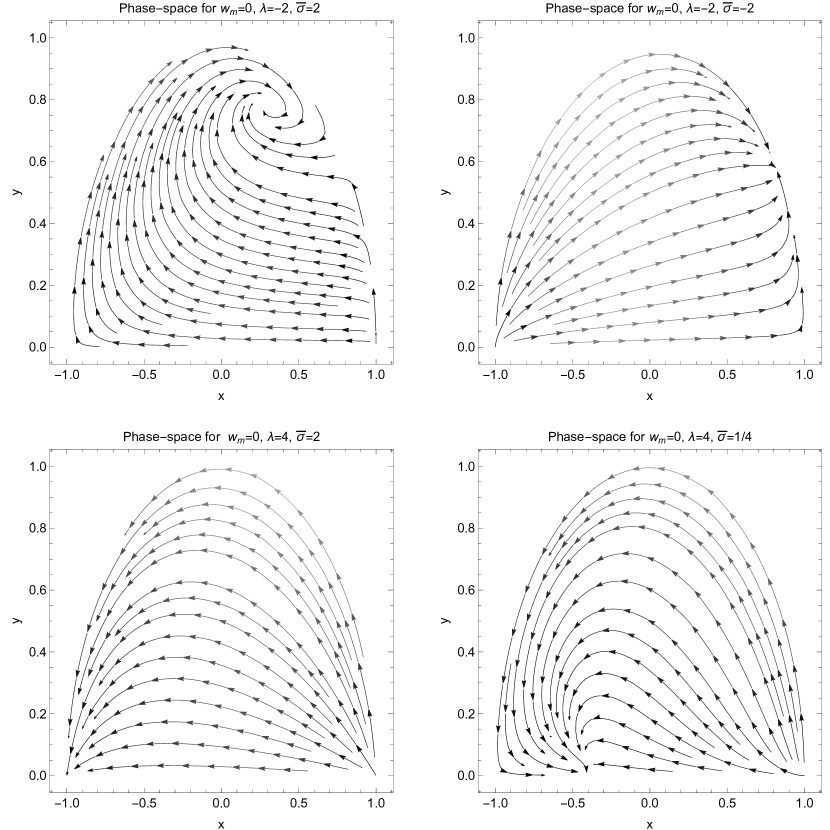
Figure 3: Phase-space portraits of the dynamical system (23), (24) of Model A for $w_{m}=0$. The free parameters have been selected such that the four stationary points appear as attractors for different values of the free parameters. For $\left(\lambda,\bar{\sigma}\right)=\left(-2,2\right)$, point $A_{4}$ is the unique attractor; for $\left(\lambda,\bar{\sigma}\right)=\left(-2,-2\right)$, point $A_{3}$ is the attractor of the dynamical system. Moreover for $\left(\lambda,\bar{\sigma}\right)=\left(4,2\right)$ point $A_{1}^{-}$ is an attractor while for $\left(\lambda,\bar{\sigma}\right)=\left(4,\frac{1}{4}\right)$ point $A_{3}$ is the attractor of the dynamical system.

Figure 4: Qualitative evolution for the effective equation of state parameter $w_{eff}\left(a\right)$ as it is given by the numerical solution of the dynamical system (23), (24) of Model A for different values of the free parameters.

Figure 5: Qualitative evolution for the $\Omega_{m}\left(a\right)$ as it is given by the numerical solution of the dynamical system (23), (24) of Model A for different values of the free parameters and the same initial conditions with Fig. 4.

In Table 1 we summarize the stationary points and their physical properties for Model A.

Table 1: Stationary points and physical properties for Model A

Point	$\left(\mathbf{x,y}\right)$	$\Omega_{m}$	$\mathbf{w}_{eff}$	Can be Attractor?
$A_{1}^{\pm}$	$\left(\pm 1,0\right)$	$0$	$1$	Yes
$A_{2}$	$\left(-\frac{\lambda}{\sqrt{6}},\sqrt{1-\frac{\lambda^{2}}{6}}\right)$	$0$	$-1+\frac{\lambda^{2}}{3}$	Yes
$A_{3}$	$\left(-\sqrt{\frac{2}{3}}\frac{1+\alpha}{1-w_{m}}\sigma,0\right)$	$1-\frac{2\bar{\sigma}^{2}}{3\left(1-w_{m}\right)^{2}}$	$\frac{2\bar{\sigma}^{2}}{3\left(1-w_{m}\right)}+w_{m}$	Yes
$A_{4}$	$\left(-\sqrt{\frac{3}{2}}\frac{1+w_{m}}{\lambda-\bar{\sigma}},\frac{\sqrt{\frac{3\left(w_{m}^{2}-1\right)}{\bar{\sigma}-\lambda}+2\bar{\sigma}}}{\sqrt{2\lambda-2\bar{\sigma}}}\right)$	$\frac{\lambda\left(\bar{\sigma}-\lambda_{0}\right)-3\left(1+w_{m}\right)}{\left(\lambda-\bar{\sigma}\right)^{2}}$	$\frac{\bar{\sigma}+w_{m}\lambda}{\lambda-\bar{\sigma}}$	Yes Always

V Model B: $V\left(\phi\right)=V_{0}e^{\lambda_{0}\phi}+\Lambda$ and $f\left(\phi\right)=f_{0}e^{\sigma_{0}\phi}$

For the second model of our consideration we consider the scalar field potential $V\left(\phi\right)=V_{0}e^{\lambda_{0}\phi}+\Lambda$ and the coupling functions $f\left(\phi\right)=f_{0}e^{\sigma_{0}\phi}.$ We calculate $\sigma=\sigma_{0},$ which means that $\sigma$ is always a constant, but now $\lambda$ is a varying parameter defined as $\lambda=\frac{V_{0}\lambda_{0}e^{\lambda_{0}\phi}}{V_{0}\lambda_{0}e^{\lambda_{0}\phi}+\Lambda}$, that is, $\phi=\frac{1}{\lambda_{0}}\ln\left(\frac{\lambda\Lambda}{V_{0}\left(\lambda_{0}-\lambda\right)}\right)$. This transformation is valid for $\frac{\lambda\Lambda}{V_{0}\left(\lambda_{0}-\lambda\right)}>0$. Moreover, we calculate $\Gamma\left(\lambda\right)=\frac{\lambda_{0}}{\lambda}$.

We end with the three-dimensional system

$$\frac{dx}{d\tau}=\frac{1}{2}\left(3x\left(x^{2}-y^{2}-1+w_{m}\left(1-x^{2}-y^{2}\right)\right)-\sqrt{6}\left(\lambda y^{2}+\left(1+\alpha\right)\sigma\left(1-x^{2}-y^{2}\right)\right)\right),$$ (25)

$$\frac{dy}{d\tau}=\frac{1}{2}y\left(3+\sqrt{6}\lambda x+3\left(x^{2}-y^{2}+w_{m}\left(1-x^{2}-y^{2}\right)\right)\right),$$ (26)

$$\frac{d\lambda}{d\tau}=\sqrt{6}x\lambda\left(\lambda_{0}-\lambda\right).$$ (27)

The stationary points $B=\left(x\left(B\right),y\left(B\right),\lambda\left(B\right)\right)$ of this dynamical system and their physical properties are discussed in the following lines.

$$B_{1}^{\pm}=\left(\pm 1,0,\lambda_{0}\right),$$

they have similar physical properties with that of $A_{1}^{\pm}$, that is, $\Omega_{m}\left(B_{1}^{\pm}\right)=0$ and $w_{eff}\left(B_{1}^{\pm}\right)=1$. As far as the stability properties of the points are concerned, we derive the eigenvalues for the linearised system $e_{1}\left(B_{1}^{\pm}\right)=\frac{\left(6+\sqrt{6}\lambda_{0}\right)}{2}$, $e_{2}\left(B_{1}^{\pm}\right)=\mp\sqrt{6}\lambda_{0}$ and $e_{3}\left(B_{1}^{\pm}\right)=3\left(1-w_{m}\right)\pm\sqrt{6}\bar{\sigma}$, with $\bar{\sigma}=\left(1+\alpha\right)\sigma$; from which we infer that the stationary points cannot describe stable solutions. Specifically for $-\sqrt{6}<\lambda<0$ and $-\sqrt{6}\bar{\sigma}<3\left(1-w_{m}\right)$ point $B_{1}^{+}$ is a source, while for $0<\lambda<\sqrt{6}$ and $\sqrt{6}\bar{\sigma}<3\left(1-w_{m}\right)$ point $B_{1}^{-}$ is a source. For other values of the free parameters points $B_{1}^{\pm}$ are saddle points.

$$B_{2}=\left(-\frac{\lambda_{0}}{6},\sqrt{1-\frac{\lambda_{0}^{2}}{6}},\lambda_{0}\right)$$

is the extension of point $A_{2}$ in the three-dimensional space. Therefore the physical properties and the existence conditions are the same. The eigenvalues are derived to be $e_{1}\left(B_{2}\right)=\frac{\left(\lambda_{0}^{2}-6\right)}{2}$, $e_{2}\left(B_{2}\right)=-3\left(1+w_{m}\right)+\lambda_{0}\left(\lambda_{0}-\bar{\sigma}\right)$ and $e_{3}\left(B_{2}\right)=\lambda_{0}^{2}$. Therefore, for $\lambda_{0}^{2}>6$ and $\lambda_{0}\bar{\sigma}<-3\left(1+w_{m}\right)+\lambda_{0}^{2}$ the stationary point is a source. Otherwise it is a saddle point.

$$B_{3}=\left(-\sqrt{\frac{2}{3}}\frac{\bar{\sigma}}{1-w_{m}},0,\lambda_{0}\right),$$

has the same physical properties as point $A_{3}$. The corresponding eigenvalues are $e_{1}\left(B_{3}\right)=-\frac{3}{2}\left(1-w_{m}\right)+\frac{\bar{\sigma}^{2}}{1-w_{m}}$ and $e_{2}\left(B_{3}\right)=\frac{3}{2}\left(1+w_{m}\right)+\frac{\bar{\sigma}\left(\bar{\sigma}-\lambda\right)}{1-w_{m}}$ and $e_{3}\left(B_{3}\right)=\frac{2\lambda_{0}\bar{\sigma}}{1-w_{m}}$. We conclude that the stationary point, when it exists, is always a saddle point.

$$B_{4}=\left(-\sqrt{\frac{3}{2}}\frac{1+w_{m}}{\lambda_{0}-\bar{\sigma}},\frac{\sqrt{\frac{3\left(w_{m}^{2}-1\right)}{\bar{\sigma}-\lambda_{0}}+2\bar{\sigma}}}{\sqrt{2\lambda_{0}-2\bar{\sigma}}},\lambda_{0}\right),$$

with asymptotic solution $\Omega_{m}\left(B_{4}\right)=\frac{\lambda\left(\bar{\sigma}-\lambda_{0}\right)-3\left(1+w_{m}\right)}{\left(\lambda-\bar{\sigma}\right)^{2}}$ and $w_{eff}\left(A_{4}\right)=\frac{\bar{\sigma}+w_{m}\lambda_{0}}{\lambda-\bar{\sigma}}$ and eigenvalues $e_{1,2}\left(B_{4}\right)=e_{1,2}\left(A_{4}\right)$ and $e_{3}=\frac{3\left(1-w_{m}\right)\lambda_{0}}{\lambda_{0}-\bar{\sigma}}$. The stability conditions are similar to those for the point $A_{4}$. Indeed, when point $B_{4}$ exists, it is is always an attractor.

$$B_{5}=\left(0,1,0\right),$$

describes a de Sitter universe with $\Omega_{m}\left(B_{5}\right)=0$ and $w_{eff}\left(B_{5}\right)=-1$. The eigenvalues are $e_{1}\left(B_{5}\right)=-3$, $e_{2}\left(B_{5}\right)=-3\left(1+w_{m}\right)$ and $e_{3}\left(B_{5}\right)=0$. Because of the zero eigenvalue we cannot infer about the stability of the dynamical system. However, we know that it may have a stable submanifold. Indeed on the surface $\lambda_{0}=0$, the stationary point is always an attractor. That is observed in Fig. 6. The analytic submanifold may be derived with the use of the center manifold theorem, but for simplicity we omit such analysis. However for equation (27) and $\lambda=\varepsilon\lambda_{\varepsilon}$, $\varepsilon^{2}\rightarrow 0$, it follows $\frac{d\lambda_{\varepsilon}}{d\tau}=\sqrt{6}x\lambda_{0}\lambda_{\varepsilon}.$ Therefore for $x\lambda_{0}>0$, $\lambda_{\varepsilon}$ increases. Otherwise for $x\lambda_{0}<0$, $\lambda_{\varepsilon}$ decays.

Furthermore, in Fig. 7 we present the phase-space portraits for the three-dimensional dynamical system (25), (26) and (27) for $\lambda_{0}=-1$, $w_{m}=0$ and $\bar{\sigma}^{2}=2$. We conclude that for initial conditions with $\lambda\leq 0$ the de Sitter universe described by $B_{5}$ is a future attractor in the surface $x\lambda_{0}<0$.

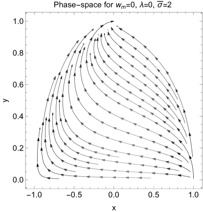
Figure 6: Phase-space portrait of the dynamical system (25), (26) and (27) of Model B on the two-dimensional surface $\lambda=0$, for $w_{m}=0$ from which it follows that the de Sitter universe is a future attractor for the dynamical system.

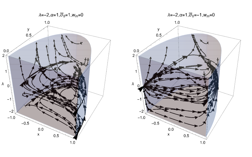
Figure 7: Phase-space portraits of the dynamical system (25), (26) and (27) of Model B for $w_{m}=0$ and $\lambda_{0}=-1$, $\bar{\sigma}=2$ (left fig.) and $\bar{\sigma}=-2$ (right fig.) From the plots we observe that for initial conditions with $\lambda<0$, the de Sitter universe is a future attractor.

V.1 Analysis at Infinity

For the dynamical system (25), (26) and (27) variables $x$ and $y$ are constrained by the algebraic condition $x^{2}+y^{2}\leq 1$, but that is not true for the dynamical variable $\lambda$ which can take values at infinity, as can be observed by Fig. 7. In order to investigate the existence of stationary points at the infinity we define the new variable $\lambda=\frac{\lambda_{b}}{\sqrt{1-\lambda_{b}^{2}}}$, from which it follows that infinity is reached when $\lambda_{b}^{2}=1$. We define the new independent variable $d\tau=\sqrt{1-\lambda_{b}^{2}}d\bar{\tau}$ , that is, at infinity the dynamical system (25), (26) and (27) becomes

$$\frac{dx}{d\bar{\tau}}=\mp\frac{\sqrt{6}}{2}y^{2}~{},~{}\frac{dy}{d\bar{\tau}}=\pm\frac{\sqrt{6}}{2}xy~{}\text{,}~{}\frac{d\lambda_{b}}{d\bar{\tau}}=\sqrt{6}x,~{}\text{for }\lambda_{b}\rightarrow\pm 1.$$ (28)

Therefore, at infinity there exists the unique stationary point $B_{\inf}=\left(0,0,\lambda_{b}\rightarrow\pm 1\right)$, which describes a matter dominated universe, $\Omega_{m}\left(B_{\inf}\right)=1$ and $w_{eff}\left(B_{\inf}\right)=w_{m}.$ From (28) it is easy to see that the stationary point at infinity is a homothetic center in the surface $\lambda_{b}^{2}=1$. However, for $x>0$, $\frac{d\lambda_{b}}{d\bar{\tau}}>0$ while for $x<0$, $\frac{d\lambda_{b}}{d\bar{\tau}}<0$, from which we can easily infer that point $B_{\inf}$ is always a saddle point.

In Table 2 we summarize the results for Model B.

Table 2: Stationary points and physical properties for Model B

Point	$\left(\mathbf{x,y,\lambda}\right)$	$\Omega_{m}$	$\mathbf{w}_{eff}$	Can be Attractor?
$B_{1}^{\pm}$	$\left(\pm 1,0,\lambda_{0}\right)$	$0$	$1$	No
$B_{2}$	$\left(-\frac{\lambda}{\sqrt{6}},\sqrt{1-\frac{\lambda^{2}}{6}},\lambda_{0}\right)$	$0$	$-1+\frac{\lambda_{0}^{2}}{3}$	No
$B_{3}$	$\left(-\sqrt{\frac{2}{3}}\frac{1+\alpha}{1-w_{m}}\sigma,0,\lambda_{0}\right)$	$1-\frac{2\bar{\sigma}^{2}}{3\left(1-w_{m}\right)^{2}}$	$\frac{2\bar{\sigma}^{2}}{3\left(1-w_{m}\right)}+w_{m}$	No
$B_{4}$	$\left(-\sqrt{\frac{3}{2}}\frac{1+w_{m}}{\lambda-\bar{\sigma}},\frac{\sqrt{\frac{3\left(w_{m}^{2}-1\right)}{\bar{\sigma}-\lambda}+2\bar{\sigma}}}{\sqrt{2\lambda-2\bar{\sigma}}},\lambda_{0}\right)$	$\frac{\lambda\left(\bar{\sigma}-\lambda_{0}\right)-3\left(1+w_{m}\right)}{\left(\lambda-\bar{\sigma}\right)^{2}}$	$\frac{\bar{\sigma}+w_{m}\lambda}{\lambda_{0}-\bar{\sigma}}$	Yes Always
$B_{5}$	$\left(0,1,0\right)$	$0$	$-1$	Yes
$B_{\inf}$	$\left(0,0,\lambda\rightarrow\pm\infty\right)$	$1$	$w_{m}$	No

VI Model C: $V\left(\phi\right)=V_{0}e^{\lambda\phi}$ and $f\left(\phi\right)=f_{0}e^{\sigma_{0}\phi}+\Lambda$

For the third model we assume that the scalar field potential and the coupling functions are $V\left(\phi\right)=V_{0}e^{\lambda\phi}$ and $f\left(\phi\right)=V_{0}e^{\sigma_{0}\phi}+\Lambda$. Therefore, we have the three-dimensional dynamical system

$$\frac{dx}{d\tau}=\frac{1}{2}\left(3x\left(x^{2}-y^{2}-1+w_{m}\left(1-x^{2}-y^{2}\right)\right)-\sqrt{6}\left(\lambda y^{2}+\left(1+\alpha\right)\sigma\left(1-x^{2}-y^{2}\right)\right)\right),$$ (29)

$$\frac{dy}{d\tau}=\frac{1}{2}y\left(3+\sqrt{6}\lambda x+3\left(x^{2}-y^{2}+w_{m}\left(1-x^{2}-y^{2}\right)\right)\right),$$ (30)

$$\frac{d\sigma}{d\tau}=\sqrt{6}x\sigma\left(\sigma_{0}-\sigma\right),$$ (31)

where $\lambda$ is a constant parameter. The stationary points $C=\left(x\left(C\right),y\left(C\right),\sigma\left(C\right)\right)$ of this dynamical system are given below.

$$C_{1}^{\pm}=\left(\pm 1,0,0\right),$$

with physical properties similar to those of points $A_{1}^{\pm}$. The eigenvalues of the linearised system are $e_{1}\left(C_{1}^{\pm}\right)=3\pm\sqrt{\frac{3}{2}}\lambda$, $e_{2}\left(C_{1}^{\pm}\right)=3\left(1-w_{m}\right)\pm\sqrt{6}\bar{\sigma}_{0}$ and $e_{3}\left(C_{1}^{\pm}\right)=\mp\frac{\sqrt{6}\bar{\sigma}_{0}}{\left(1+\alpha\right)}$; in which $\bar{\sigma}_{0}=\sigma_{0}\left(1+\alpha\right)$ and $\bar{\sigma}=\sigma\left(1+\alpha\right)$. Therefore, $A_{1}^{+}$ is an attractor for $\lambda<-\sqrt{6}$, $\bar{\sigma}_{0}>\frac{3}{\sqrt{6}}\left(1-w_{m}\right)$ and $\frac{\sqrt{6}\bar{\sigma}_{0}}{\left(1+\alpha\right)}>0$. On the other hand point $A_{1}^{-}$ is an attractor for $\lambda>\sqrt{6}$, $\bar{\sigma}_{0}<\frac{3}{\sqrt{6}}\left(1-w_{m}\right)$ and $\frac{\sqrt{6}\bar{\sigma}_{0}}{\left(1+\alpha\right)}<0$.

$$C_{2}=\left(-\frac{\lambda}{\sqrt{6}},\sqrt{1-\frac{\lambda^{2}}{6}},\bar{\sigma}_{0}\right),$$

with $\Omega\left(C_{2}\right)=0$ and $w_{eff}\left(C_{2}\right)=1+\frac{\lambda^{2}}{3}$. Indeed, point $C_{2}$ is the extension of $A_{2}$ in the three-dimensional manifold of variables $\left\{x,y,\sigma\right\}$. We calculate the eigenvalues $e_{1}\left(C_{2}\right)=\frac{\left(\lambda^{2}-6\right)}{2}$, $e_{2}\left(C_{2}\right)=-3\left(1+w_{m}\right)+\lambda\left(\lambda-\sigma_{0}\right)$ and $e_{3}\left(C_{2}\right)=\frac{\lambda\bar{\sigma}_{0}}{1+\alpha}$. Hence for $\lambda^{2}<6$, $\frac{\lambda\bar{\sigma}_{0}}{1+\alpha}<0$ and $3\left(1+w_{m}\right)+\lambda\left(\lambda-\sigma_{0}\right)<0$ the stationary point is an attractor.

$$C_{3}=\left(-\sqrt{\frac{2}{3}}\frac{\bar{\sigma}_{0}}{1-w_{m}},0,\sigma_{0}\right),$$

with physical variables $\Omega_{m}\left(C_{3}\right)=1-\frac{2\bar{\sigma}_{0}^{2}}{3\left(1-w_{m}\right)^{2}}$ and $w_{eff}\left(C_{3}\right)=\frac{2\bar{\sigma}_{0}^{2}}{3\left(1-w_{m}\right)}+w_{m}$. The eigenvalues are calculated $e_{1}\left(C_{1}\right)=-\frac{3}{2}\left(1-w_{m}\right)+\frac{\bar{\sigma}_{0}^{2}}{1-w_{m}},~{}e_{2}\left(C_{3}\right)=\frac{3}{2}\left(1+w_{m}\right)-\frac{\bar{\sigma}_{0}\left(\lambda-\bar{\sigma}_{0}\right)}{\left(1-w_{m}\right)}$ and $e_{3}\left(C_{3}\right)=\frac{2\left(\bar{\sigma}_{0}\right)^{2}}{\left(1-w_{m}\right)\left(1+\alpha\right)}$. Therefore $C_{3}$ describes a stable solution and $C_{3}$ is an attractor for $\alpha<-1$ and $\sqrt{6}\left|\sigma_{0}\right|<3\left(1-w_{m}\right),$ $\lambda+\frac{3\left(w_{m}^{2}-1\right)}{2\left|\bar{\sigma}_{0}\right|}<\left|\bar{\sigma}_{0}\right|$.

$$C_{4}=\left(-\sqrt{\frac{3}{2}}\frac{1+w_{m}}{\lambda_{0}-\bar{\sigma}},\frac{\sqrt{\frac{3\left(w_{m}^{2}-1\right)}{\bar{\sigma}-\lambda_{0}}+2\bar{\sigma}}}{\sqrt{2\lambda_{0}-2\bar{\sigma}}},\sigma_{0}\right),$$

is the extension of point $A_{4}$ in the three-dimensional space. The eigenvalues are $e_{1,2}\left(C_{4}\right)=e_{1,2}\left(A_{4}\right)$ and $e_{3}=\frac{3\left(1+w_{m}\right)\bar{\sigma}_{0}}{\left(1+\alpha\right)\left(\lambda-\bar{\sigma}_{0}\right)}$ from which we can easily conclude that, when the point exist, is is always an attractor. Similarly to the property of points $A_{4}$ and $B_{4}$.

$$C_{5}=\left(0,0,0\right)$$

describes a universe dominated by the ideal gas, that is, $\Omega_{m}\left(C_{5}\right)=1$ and $w_{eff}\left(C_{5}\right)=w_{m}.$ That is the new point provided by the coupling function $f\left(\phi\right)=V_{0}e^{\sigma_{0}\phi}+\Lambda$. By definition $\phi=\frac{1}{\sigma_{0}}\ln\left(\frac{\sigma\Lambda}{f_{0}\left(\sigma-\sigma_{0}\right)}\right)$, that is, the limit $\sigma_{0}$ means that $\phi\rightarrow-\infty$. Therefore, for $\sigma=0$, the coupling function becomes $f\left(\phi\right)\rightarrow\Lambda.$ The eigenvalues of the linearised system are $e_{1}\left(C_{5}\right)=-\frac{3}{2}\left(1+w_{m}\right)$, $e_{2}\left(C_{5}\right)=\frac{3}{2}\left(1-w_{m}\right)$ and $e_{3}\left(C_{5}\right)=0$, from which we infer that point $C_{5}$ describes always an unstable asymptotic solution and $C_{5}$ is a saddle point.

In Fig. 8 we present three-dimensional phase-space portraits of the dynamical system (29), (30) and (31) for different values of the free parameters.

Figure 8: Phase-space portraits of the dynamical system (29), (30) and (31) of Model C, for different values of the free parameters.

In Fig. 9 we present the qualitative evolution of the effective equation of state for various values of the free parameters for this model. We observe that for $w_{m}=0$, if we start for initial conditions near to the radiation epoch, this model can reconstruct the cosmological history of the late universe. Moreover, the evolution of $\Omega_{m}$ is presented in Fig. 10. For the initial conditions of the latter figures we considered the radiation epoch, that is, the effective fluid mimics the radiation fluid. The trajectories go near to the saddle point which describes the matter era and end at a universe dominated by the scalar field.

Figure 9: Qualitative evolution for the effective equation of state parameter $w_{eff}\left(a\right)$ as it is given by the numerical solution of the dynamical system (29), (30) and (31) of Model C for different values of the free parameters.

Figure 10: Qualitative evolution for $\Omega\left(a\right)$ as it is given by the numerical solution of the dynamical system (29), (30) and (31) of Model C for different values of the free parameters and the same initial conditions with that of Fig. 9

VI.1 Analysis at Infinity

We apply the same procedure as for the Model B where now we consider the variables $\sigma=\frac{\sigma_{b}}{\sqrt{1-\sigma_{b}^{2}}}$ and $d\tau=\sqrt{1-\sigma_{b}^{2}}d\bar{\tau}$. At the limit of infinity the dynamical system becomes

$$\frac{dx}{d\bar{\tau}}=\pm\frac{\sqrt{6}}{2}\left(1+\alpha\right)\left(x^{2}+y^{2}-1\right),~{}\frac{dy}{d\bar{\tau}}=0\text{ , }\frac{d\sigma_{b}}{d\bar{\tau}}=\sqrt{6}x~{}\text{for }\sigma_{b}\rightarrow\pm 1,$$ (32)

from which it follows the stationary point $C_{\inf}=\left(0,1,\sigma_{b}^{2}\rightarrow 1\right)$. Point $C_{\inf}$ describes a de Sitter universe with $\Omega_{m}\left(C_{\inf}\right)=0$ and $w_{eff}\left(C_{\inf}\right)=-1$. Similarly as before we conclude that the stationary point describes an unstable solution.

We summarize the results of this Section in Table 3.

Table 3: Stationary points and physical properties for Model C

Point	$\left(\mathbf{x,y,\sigma}\right)$	$\Omega_{m}$	$\mathbf{w}_{eff}$	Can be Attractor?
$C_{1}^{\pm}$	$\left(\pm 1,0,\sigma_{0}\right)$	$0$	$1$	Yes
$C_{2}$	$\left(-\frac{\lambda_{0}}{\sqrt{6}},\sqrt{1-\frac{\lambda_{0}^{2}}{6}},\sigma_{0}\right)$	$0$	$-1+\frac{\lambda^{2}}{3}$	Yes
$C_{3}$	$\left(-\sqrt{\frac{2}{3}}\frac{1+\alpha}{1-w_{m}}\sigma,0,\sigma_{0}\right)$	$1-\frac{2\bar{\sigma}^{2}}{3\left(1-w_{m}\right)^{2}}$	$\frac{2\bar{\sigma}^{2}}{3\left(1-w_{m}\right)}+w_{m}$	Yes
$C_{4}$	$\left(-\sqrt{\frac{3}{2}}\frac{1+w_{m}}{\lambda_{0}-\bar{\sigma}},\frac{\sqrt{\frac{3\left(w_{m}^{2}-1\right)}{\bar{\sigma}-\lambda}+2\bar{\sigma}}}{\sqrt{2\lambda_{0}-2\bar{\sigma}}},\sigma_{0}\right)$	$\frac{\lambda\left(\bar{\sigma}-\lambda_{0}\right)-3\left(1+w_{m}\right)}{\left(\lambda-\bar{\sigma}\right)^{2}}$	$\frac{\bar{\sigma}_{0}+w_{m}\lambda}{\lambda-\bar{\sigma}_{0}}$	Yes Always
$C_{5}$	$\left(0,0,0\right)$	$1$	$w_{m}$	No
$C_{\inf}$	$\left(0,1,\sigma\rightarrow\pm\infty\right)$	$0$	$-1$	No

VII Model D: $V\left(\phi\right)=V_{0}e^{\lambda_{0}\phi}+\Lambda$ and $f\left(\phi\right)=f_{0}\left(V_{0}e^{\lambda_{0}\phi}+\Lambda\right)^{p}$

Consider now the cosmological model with scalar field potential $V\left(\phi\right)=V_{0}e^{\lambda_{0}\phi}+\Lambda$ and coupling function for the chameleon mechanism $f\left(\phi\right)=f_{0}\left(V\left(\phi\right)\right)^{p}$. For these functions it follows that $\sigma\left(\lambda\right)=p\lambda$. Thus, the field equations are expressed by the following three-dimensional system

$$\frac{dx}{d\tau}=\frac{1}{2}\left(3x\left(x^{2}-y^{2}-1+w_{m}\left(1-x^{2}-y^{2}\right)\right)-\sqrt{6}\left(\lambda y^{2}+\lambda\bar{p}\left(1-x^{2}-y^{2}\right)\right)\right),$$ (33)

$$\frac{dy}{d\tau}=\frac{1}{2}y\left(3+\sqrt{6}\lambda x+3\left(x^{2}-y^{2}+w_{m}\left(1-x^{2}-y^{2}\right)\right)\right),$$ (34)

$$\frac{d\lambda}{d\tau}=\sqrt{6}x\lambda\left(\lambda_{0}-\lambda\right),$$ (35)

where $\bar{p}=\left(1+\alpha\right)p$. In the following lines we derive the stationary points of this system and we discuss their stability properties.

$$D_{1}=\left(\pm 1,0,\lambda_{0}\right),$$

have similar physical properties as points $A_{1}^{\pm}$. We calculate the eigenvalues $e_{1}\left(D_{1}^{\pm}\right)=\frac{\left(6+\sqrt{6}\lambda_{0}\right)}{2}$, $e_{2}\left(D_{1}^{\pm}\right)=\mp\sqrt{6}\lambda_{0}$ and $e_{3}\left(D_{1}^{\pm}\right)=3\left(1-w_{m}\right)\pm\sqrt{6}\bar{p}\lambda_{0}$,  from which it follows that for $\bar{p}\left|\lambda_{0}\right|<\frac{3\left(1-w_{m}\right)}{\sqrt{6}}$, point $D_{1}^{+}$ is a source when $-\sqrt{6}<\lambda<0$, while point $D_{1}^{-}$ is a source for $0<\lambda<\sqrt{6}$. Otherwise the two points are saddle points.

$$D_{2}=\left(-\frac{\lambda_{0}}{6},\sqrt{1-\frac{\lambda_{0}^{2}}{6}},\lambda_{0}\right),$$

with eigenvalues $e_{1}\left(D_{2}\right)=\frac{\left(\lambda_{0}^{2}-6\right)}{2}$, $e_{2}\left(D_{2}\right)=-3\left(1+w_{m}\right)+\lambda_{0}\left(\lambda_{0}-\bar{p}\lambda_{0}\right)$ and $e_{3}\left(D_{2}\right)=\lambda_{0}^{2}$ describes an unstable scaling solution similar to that of point $B_{2}$ with the same stability properties, by replacing $\bar{\sigma}=\bar{p}\lambda_{0}$.

$$D_{3}=\left(-\sqrt{\frac{2}{3}}\frac{\bar{p}\lambda_{0}}{1-w_{m}},0,\lambda_{0}\right).$$

it is point $B_{3}$ and it has the same physical and stability properties as for $\bar{\sigma}=\bar{p}\lambda_{0}$.

$$D_{4}=\left(-\sqrt{\frac{3}{2}}\frac{1+w_{m}}{\lambda_{0}-\bar{p}\lambda_{0}},\frac{\sqrt{\frac{3\left(w_{m}^{2}-1\right)}{\bar{p}\lambda_{0}-\lambda_{0}}+2\bar{p}\lambda_{0}}}{\sqrt{2\lambda_{0}-2\bar{p}\lambda_{0}}},\lambda_{0}\right).$$

it is point $B_{4}$ for $\bar{\sigma}=\bar{p}\lambda_{0}$, and it has the same physical and stability properties, that is, point $D_{4}$ is an attractor when it exists.

$$D_{5}=\left(0,0,0\right),$$

it is an asymptotic solution in which the matter source dominates in the universe similarly to point $C_{5}$ with the same eigenvalues. Hence, point $D_{5}$ is always a saddle point.

$$D_{6}=\left(0,1,0\right),$$

describes a de Sitter universe similar to point $B_{5}$ for which the cosmological constant term dominates in the scalar field potential. The stability properties are similar with those of point $B_{5}$.

In Fig. 11 we present the three-dimensional phase-space portrait for the dynamical system (33), (34) and (35) of Model D. Furthermore, the qualitative evolution of the effective equation of state parameter $w_{eff}~{}$is given in Fig. 12 and the dynamical evolution of $\Omega_{m}$ is presented in Fig. 13. From this we have selected a set of initial conditions whereby the dynamical system can describe the main eras of the cosmological history. We observe that a main difference of the evolution of $w_{eff}$ with that of Model C is that now the future attractor can be a de Sitter universe, i.e. point $D_{6}$, instead of a scaling solution described by point $C_{4}$. For the initial conditions of the latter figures we considered the effective fluid to describe radiation. From the evolution of the trajectories we observe that the universe goes near to the saddle point which describes the matter era and ends to a universe dominated by the scalar field which is a future attractor.

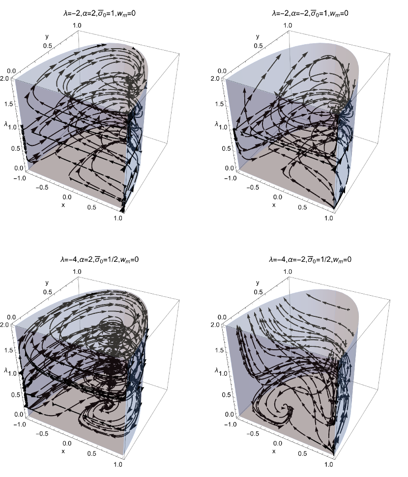
Figure 11: Phase-space portraits of the dynamical system (33), (34) and (35) of Model D, for different values of the free parameters.

Figure 12: Qualitative evolution for the effective equation of state parameter $w_{eff}\left(a\right)$ as it is given by the numerical solution of the dynamical system (33), (34) and (35) of model D for different values of the free parameters.

Figure 13: Qualitative evolution for $\Omega_{m}\left(a\right)$ as given by the numerical solution of the dynamical system (33), (34) and (35) of model D for different values of the free parameters and the same initial conditions with that of Fig. 12

VII.1 Analysis at Infinity

For the analysis at infinity we apply the same procedure as that for Model B. At infinity, i.e. $\lambda_{b}^{2}\rightarrow 1$, we end with the dynamical system

$$\frac{dx}{d\bar{\tau}}=\mp\frac{\sqrt{6}}{2}\left(\bar{p}\left(1-x^{2}\right)+\left(1-\bar{p}\right)y^{2}\right)~{},~{}\frac{dy}{d\bar{\tau}}=\pm\frac{\sqrt{6}}{2}xy~{}\text{,}~{}\frac{d\lambda_{b}}{d\bar{\tau}}=\sqrt{6}x~{},$$ (36)

which means that the unique stationary point for $\bar{p}\neq 1$ is the $D_{\inf}=\left(0,\sqrt{\frac{\bar{p}}{\bar{p}-1}},\lambda_{b}\rightarrow\pm 1\right).$ For that stationary point we derive $\Omega\left(D_{\inf}\right)=0$ and $w_{eff}\left(D_{\inf}\right)=-1$, which means that it describes a de Sitter solution. On the surface $\lambda_{b}^{2}=1$ the point is a homothetic center. However, from the differential equation for the variable $\lambda_{b}$ it follows that $D_{\inf}$ is always a saddle point. For $\bar{p}=1$, there exists a family of saddle stationary points $\bar{D}_{\inf}=\left(0,y,\lambda_{b}\rightarrow\pm 1\right)$ which describe solutions with $\Omega\left(\bar{D}_{\inf}\right)=1-y^{2}\left(\bar{D}\right)$ and$~{}w_{eff}\left(\bar{D}\right)=w_{m}\left(1-y^{2}\left(\bar{D}\right)\right)-y^{2}\left(\bar{D}\right)$.

That is a very interesting result because Model D can provide two de Sitter epochs one unstable at infinity,in which can be related to inflation, and one attractor related to the late-time acceleration phase.

The stability analysis for Model D is summarized in Table 4

Table 4: Stationary points and physical properties for Model D

Point	$\left(\mathbf{x,y,\lambda}\right)$	$\Omega_{m}$	$\mathbf{w}_{eff}$	Can be Attractor?
$D_{1}^{\pm}$	$\left(\pm 1,0,\lambda_{0}\right)$	$0$	$1$	No
$D_{2}$	$\left(-\frac{\lambda}{\sqrt{6}},\sqrt{1-\frac{\lambda^{2}}{6}},\lambda_{0}\right)$	$0$	$-1+\frac{\lambda_{0}^{2}}{3}$	No
$D_{3}$	$\left(-\sqrt{\frac{2}{3}}\frac{1+\alpha}{1-w_{m}}\sigma,0,\lambda_{0}\right)$	$1-\frac{2\bar{\sigma}^{2}}{3\left(1-w_{m}\right)^{2}}$	$\frac{2\bar{\sigma}^{2}}{3\left(1-w_{m}\right)}+w_{m}$	No
$D_{4}$	$\left(-\sqrt{\frac{3}{2}}\frac{1+w_{m}}{\lambda-\bar{\sigma}},\frac{\sqrt{\frac{3\left(w_{m}^{2}-1\right)}{\bar{\sigma}-\lambda}+2\bar{\sigma}}}{\sqrt{2\lambda-2\bar{\sigma}}},\lambda_{0}\right)$	$1-\frac{2\bar{\sigma}^{2}}{3\left(1-w_{m}\right)^{2}}$	$\frac{\bar{\sigma}+w_{m}\lambda}{\lambda_{0}-\bar{\sigma}}$	Yes Always
$D_{5}$	$\left(0,0,0\right)$	$1$	$0$	No
$D_{6}$	$\left(0,1,0\right)$	$0$	$-1$	Yes
$D_{\inf}$	$\left(0,\sqrt{\frac{p}{p-1}},\lambda\rightarrow\pm\infty\right)$	$0$	$-1$	No
$\bar{D}_{\inf}$	$\left(0,y^{2}\left(\bar{D}\right),\lambda\rightarrow\pm\infty\right)~{},~{}$for $\bar{p}=1$	$1-y^{2}\left(\bar{D}\right)$	$w_{m}\left(1-y^{2}\left(\bar{D}\right)\right)-y^{2}\left(\bar{D}\right)$	No

VIII Conclusions

In this work we investigated the phase-space of the cosmological field equations in chameleon dark energy. In particular we performed a detailed dynamical analysis for the gravitational field equations in a spatially flat FLRW with a scalar field coupled to an ideal gas. The coupling function is responsible for the chameleon mechanism when the mass of the scalar field depends upon the energy density of the ideal  gas. In order to avoid the violation of the weak energy condition, we assumed the scalar field to be that of quintessence and the coupling function to be always of positive value. In in such a scenario the Hubble function does not change sign. Consequently, for the study of the dynamics we followed the $H$-normalization approach. We defined a new set of dimensionless variables and we expressed all the physical quantities in terms of these variables.

In the $H$-normalization approach the field equations are written in an equivalent form of an algebraic-differential system where the independent variable is the radius of the FLRW geometry, that is, the scale factor. With the use of the algebraic equation the dimensional space of the field equation is reduced to a maximum dimension of three. The dynamical evolution of the physical variables it depends on the selection of two unknown functions, the scalar field potential and the coupling function. We considered four different sets for the free functions; for these four models we discussed in details the evolution of the dynamics and the physical properties of the asymptotic solutions.

For the first cosmological model of our consideration, namely Model A, we assumed that the potential and the coupling functions are exponential, that is, $V\left(\phi\right)=V_{0}e^{\lambda_{0}\phi}$ and $f\left(\phi\right)=f_{0}e^{\sigma_{0}\phi}$. For the exponential coupling function the theory is equivalent with the Weyl Integrable Spacetime. Furthermore, the dimension of the field equations in the dimensional variables for this selection of the unknown functions is reduced to two. The admitted stationary points are four, the two points correspond to the quintessence model for which the ideal gas does not contribute to the cosmological fluid, that is, we derived the stiff fluid epoch in which the kinetic term of the scalar field contributes in the field equations and a scaling solution which can describe acceleration. On the other hand, for the remainder of the stationary points the ideal gas contributes in the cosmological fluid. These points can describe scaling solutions related to the matter or to the late-time acceleration of the universe.

Model B was considered with $V\left(\phi\right)=V_{0}e^{\lambda_{0}\phi}+\Lambda$ and $f\left(\phi\right)=f_{0}e^{\sigma_{0}\phi}$. In this case the field equations form a three-dimensional system. On the two-dimensional surface we recovered the four stationary points of Model A. Moreover we found two new stationary points which describe a Sitter universe and a matter dominated era. In order to determine the existence of the matter dominated era we had to make use of Poincare’ variables so as to investigate the asymptotic dynamics at the infinity regime. In Model C with $V\left(\phi\right)=V_{0}e^{\lambda\phi}$ and $f\left(\phi\right)=f_{0}e^{\sigma_{0}\phi}+\Lambda\,$, we determined the same stationary points as in Model B, but now the de Sitter point appeared in the infinity regime while the matter dominated solutions exist in the finite regime. It is important to mention that the stability properties are different in each model.

Finally, for the fourth-model of our consideration with $V\left(\phi\right)=V_{0}e^{\lambda_{0}\phi}+\Lambda$ and $f\left(\phi\right)=f_{0}\left(V_{0}e^{\lambda_{0}\phi}+\Lambda\right)^{p}~{}$with$~{}p\neq 0$, we calculated six stationary points at the finite regime which describe physical solutions corresponding to the stationary points at the finite regime for the cosmological Models A, B and C. Moreover, in the infinite regime for $p\neq 1$, an unstable de Sitter universe exists which can be related to the early inflationary epoch of the universe, while for $p=1$, the unstable solution at infinity describes a family of scaling solutions.

For each of the above mentioned cosmological models, we presented phase-space portraits of the dynamical variables and the qualitative evolution of the effective equation of state parameter for different sets of initial conditions and values of the free parameters. The results from the stability analysis and the phase-space portraits can be used to constrain the region of the free variables for the initial condition problem. Furthermore, from the evolution of the effective equation of state parameters we can conclude that these models can reproduce the main eras of the cosmological history. Also, Model D can be used to unify the all the components for the dark sector of the universe and it shows that it can provide a mechanism to relate the dark energy and the inflation responsible for the inflation.

In future work we plan to focus on the analysis of the perturbations and to investigate if these models can solve cosmological tensions.

References

(1)A.G. Riess et al., Observational evidence from Supernovae for an
accelerating universe and cosmological constant, Astron. J. 116, 1009 (1998)
(2)M. Tegmark et al., Astrophys. J. 606, 702 (2004)
(3)M. Kowalski et al., Astrophys. J. 686, 749 (2008)
(4)E. Komatsu et al., Astrophys. J. Suppl. Ser. 180, 330 (2009)
(5)N. Suzuki et al., Astrophys. J. 746, 85 (2012)
(6)J. Yoo and Y. Watanabe, Theoretical models of dark energy, Int.
J. Mod. Phys. D 21, 1230002 (2012)
(7)T. Clifton, P.G. Ferreira, A. Padilla and C. Skordis, Phys.
Rept. 513, 1 (2012)