Learning with a Mole: Transferable latent spatial representations for navigation without reconstruction

Abstract

Agents navigating in 3D environments require some form of memory, which should hold a compact and actionable representation of the history of observations useful for decision taking and planning. In most end-to-end learning approaches the representation is latent and usually does not have a clearly defined interpretation, whereas classical robotics addresses this with scene reconstruction resulting in some form of map, usually estimated with geometry and sensor models and/or learning. In this work we propose to learn an actionable representation of the scene independently of the targeted downstream task and without explicitly optimizing reconstruction. The learned representation is optimized by a blind auxiliary agent trained to navigate with it on multiple short sub episodes branching out from a waypoint and, most importantly, without any direct visual observation. We argue and show that the blindness property is important and forces the (trained) latent representation to be the only means for planning. With probing experiments we show that the learned representation optimizes navigability and not reconstruction. On downstream tasks we show that it is robust to changes in distribution, in particular the sim2real gap, which we evaluate with a real physical robot in a real office building, significantly improving performance.

1 Introduction

Navigation in 3D environments requires agents to build actionable representations, which we define as in Ghosh et al. (2019) as “aim(ing) to capture those factors of variation that are important for decision making”. Classically, this has been approached by integrating localization and reconstruction through SLAM (Thrun et al., 2005; Bresson et al., 2017; Lluvia et al., 2021), followed by planning on these representations. On the other end of the spectrum we can find end-to-end approaches, which map raw sensor data through latent representations directly to actions and are typically trained large-scale in simulations from reward (Mirowski et al., 2017; Jaderberg et al., 2017) or with imitation learning (Ding et al., 2019). Even for tasks with low semantics like PointGoal, it is not completely clear whether an optimal representation should be “handcrafted” or learned. While trained agents can achieve extremely high success rates of up to 99% (Wijmans et al., 2019; Partsey et al., 2022), this has been reported in simulation. Performance in real environments is far lower, and classical navigation stacks remain competitive in these settings (Sadek et al., 2022). This raises the important question of whether robust and actionable representations should be based on precise reconstruction, and we argue that an excess amount of precision can potentially lead to a higher internal sim2real gap and hurt transfer, similar (but not identical) to the effect of fidelity in training in simulation (Truong et al., 2022). Interestingly, research in psychology has shown that human vision has not been optimized for high-fidelity 3D reconstruction, but for the usefulness and survival (Prakash et al., 2021).

We argue that artificial agents should follow a similar strategy and we propose tailored auxiliary losses, which are based on interactions with the environment and directly target the main desired property of a latent representation: its usability for navigation. This goal is related to Cognitive Maps, spatial representations built by biological agents hown to emerge from interactions (Tolman, 1948; Blodgett, 1929; Menzel, 1973), even in blind agents, biological (Lumelsky & Stepanov, 1987) or artificial ones (Wijmans, 2022; Wijmans et al., 2023).

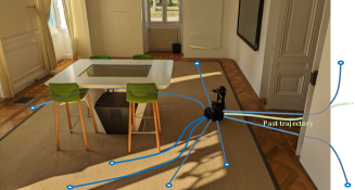
Figure 1: Without reconstruction, we learn an actionable map-like representation computed by an agent of the visual observations collected along its trajectory  . We optimize for its usefulness: a representation estimated at at point is passed to a blind auxiliary agent trained to reach subgoals on short episodes  . Solving this requires sufficient latent reconstruction of the scene, and we show that blindess of the aux agent is a key property. We train in simulation and transfer to a real environment.

Inspired by this line of research, we propose learning a latent spatial representation we call Navigability and avoid spending training signals on learning to explicitly reconstruct the scene in unnecessary detail, potentially not useful and could even harm transfer. We augment the amount of information carried by the training signal compared to reward. We consider the ability of performing local navigation an essential skill for a robot, i.e. the capability to detect free navigable space, to avoid obstacles, and to find the openings in closed spaces in order to leave them. We propose to learn a representation which optimizes these skills directly, prioritizing usability over fidelity, as shown in Figure 1. A representation is built by an agent through sequential integration of visual observations. This representation is passed to a blind auxiliary agent, which is trained to use it as its sole information to navigate to a batch of intermediate subgoals. Optimizing over the success of the blind auxiliary agent leads to an actionable representation and can be done independently of the downstream task.

We explore the following questions: (i) Can a latent cognitive map be learned by an agent through the communication with a blind auxiliary agent? (ii) What kind of spatial information does it contain? (iii) Can it be used for downstream tasks? (iv) Is it more transferable than end-to-end training in out-of-distribution situations such as sim2real transfer?

2 Related Work

Navigation with mapping and planning — Classical methods typically require a map (Burgard et al., 1998; Marder-Eppstein et al., 2010; Macenski et al., 2020) and are composed of three modules: mapping and localization using visual observations or Lidar (Thrun et al., 2005; Labbé & Michaud, 2019; Bresson et al., 2017; Lluvia et al., 2021), high-level planning (Konolige, 2000; Sethian, 1996) and low-level path planning (Fox et al., 1997; Rösmann et al., 2015). These methods depend on sophisticated noise filtering, temporal integration with precise odometry and loop closure. In comparison, we avoid the intermediate goal of explicit reconstruction, directly optimizing usefulness.

End-to-end training — on the other side of the spectrum we find methods which directly map sensor input to actions and trained latent representations, either flat vectorial like GRU memory, or structured variants: neural metric maps encoding occupancy (Chaplot et al., 2020b), semantics (Chaplot et al., 2020a) or fully latent metric representations (Parisotto & Salakhutdinov, 2018; Beeching et al., 2020b; Henriques & Vedaldi, 2018); neural topological maps  (Beeching et al., 2020a; Shah & Levine, 2022; Shah et al., 2021); transformers (Vaswani et al., 2017) adapted to navigation (Fang et al., 2019; Du et al., 2021; Chen et al., 2022; Reed et al., 2022); and implicit representations (Marza et al., 2023). While these methods share our goal of learning useful and actionable representations, these representations are tied to the actual downstream task, whereas our proposed “Navigability” optimizes for local navigation, an important capability common to all navigation tasks.

Pre-text tasks — Unsupervised learning and auxiliary tasks share a similar high-level goal with our work, they provide a richer and more direct signal for representation learning. Potential fields (Ramakrishnan et al., 2022) are trained from top down maps and contain unexplored areas and estimates of likely object positions. A similar probabilistic way has been proposed in RECON by Shah et al. (2021). In (Marza et al., 2022), goal direction is directly supervised. Our work can be seen as a pre-text task directly targeting the usefulness of the representation combined with an inductive bias in the form of the blind auxiliary agent.

Backpropagating through planning — in this line of work a downstream objective is backpropagated through a differentiable planning module to learn the upstream representation. In (Weerakoon et al., 2022) and similarly in (Dashora et al., 2021), this is a cost-map used by a classical planner. Neural-A* (Yonetani et al., 2021) learns a cost-map used by a differentiable version of A*. Similarly, Cognitive Mapping and Planning (Gupta et al., 2017) learns a mapping function by backpropagating through Value Iteration Networks (Tamar et al., 2016). Our work shares the overall objective, the difference being that (i) we optimize Navigability as an additional pre-text task and, (ii) we introduce the blind agent as inductive bias, which minimizes the reactive component of the task and strengthens the more useful temporal integration of a longer history of observations — see Section 4. Somewhat related to our work, motion planning performance has been proposed as learnable evaluation metric for metric representations of autonomous vehicles (Philion et al., 2020), and attempts have been made to leverage this kind of metric for learning representations (Philion & Fidler, 2020; Zeng et al., 2021), albeit without application to navigation.

Sim2Real transfer — transferring representations to real world has gained traction since the recent trend to large-scale learning in simulated 3D environments (Höfer et al., 2020; Chattopadhyay et al., 2021; Kadian et al., 2020; Anderson et al., 2018; Dey et al., 2023). Domain randomization randomizes the factors of variation during training (Peng et al., 2018; Tan et al., 2018), whereas domain adaptation transfers the model to real environments, or in both directions (Truong et al., 2021), through adversarial learning (Zhang et al., 2019), targeting dynamics (Eysenbach et al., 2021) or perception (Zhu et al., 2019), or by fine-tuning to the target environment (Sadek et al., 2022). Table 6 in appendix lists some efforts. Our work targets the transfer of a representation by optimizing its usefulness instead of reconstruction.

Biological agents — like rats, have been shown to build Cognitive Maps, spatial representations emerging from interactions (Tolman, 1948), shown to partially emerge even when there is no reward nor incentives (Blodgett, 1929; Tolman, 1948). Similarly, chimpanzees are capable of developing greedy search after interactions (Menzel, 1973). Blind biological agents have been shown to be able navigate (Lumelsky & Stepanov, 1987), which has recently been replicated for artificial agents (Wijmans et al., 2023). Certain biological agents have also been shown to develop grid, border and place cells (Hafting et al., 2005), which have also been reproduced in artificial agents (Cueva & Wei, 2018; Banino et al., 2018). There are direct connections to our work, where a representation emerges from interactions of a blind agent.

Goal-oriented models — are learned through optimizing an objective with respect to subgoals. Hindsight Experience Replay (Andrychowicz et al., 2017) optimizes sample efficiency by reusing unsuccessful trajectories, recasting them as successful ones wrt. different goals. Chebotar et al. (2021) learn “Actionable Models” by choosing different states in trajectories as subgoals through hindsight replay. In Reinforcement Learning (RL), successor states provide a well founded framework for goal dependent value functions (Blier et al., 2021). Subgoals have also recently been integrated into the MDP-option framework (Lo et al., 2022). Similarly, subgoals play a major part in our work.

3 Learning Navigability

We learn a representation useful for different visual navigation problems, and without loss of generality we formalize the problem as a PointGoal task: An agent receives visual observations $\mathbf{o}_{t}$ and a Euclidean goal vector $G$ at each time step $t$ and must take actions $\mathbf{a}_{t}$, which are typically discrete actions from a given alphabet $\{$FORWARD 25cm, TURN_LEFT $10^{\circ}$, TURN_RIGHT $10^{\circ}$ and STOP$\}$. The agent sequentially builds a representation $\mathbf{r}_{t}$ from the sequence of observations $\{\mathbf{o}_{t^{\prime}}\}_{t^{\prime}<t}$ and the previous action $\mathbf{a}_{t-1}$, and a policy $\pi$ predicts a distribution over actions,

$$\mathbf{r}_{t} =f(\mathbf{o}_{t},\mathbf{r}_{t-1},\mathbf{a}_{t-1}),$$ (1)

$$p(\mathbf{a}_{t}) =\pi(\mathbf{r}_{t},G),$$ (2)

where $f$ in our case is a neural network with GRU memory (Cho et al., 2014), but which can also be modeled as self-attention over time as in (Chen et al., 2021; Janner et al., 2021; Reed et al., 2022). We omit dependencies on parameters and gating mechanisms from our notations.

We do not focus on learning the main policy $\pi$, which can be trained with RL, imitation learning (IL) or other losses on a given downstream task. Instead, we address the problem of learning the representation $\mathbf{r}_{t}$ through its usefulness: we optimize the amount of information $\mathbf{r}_{t}$ carries about the navigability of (and towards) different parts of the scene. When given to a blind auxiliary agent, this information should allow the agent to navigate to any sufficiently close point, without requiring any visual observation during its own steps. We cast this as a tailored variant of behavior cloning (BC) using privileged information from the simulator.

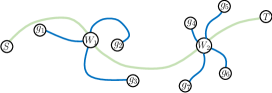
Figure 2: Our training data are organized into “long episodes” from start $S$ to target $T$ navigated by the main agent $\pi$ and “short episodes” branching out at waypoints $W_{i}$ to subgoals $g_{j}$.

We organize the training data into episodes, for each of which we suppose the existence of optimal (shortest) paths, e.g. calculated in simulation from GT maps. We distinguish between long and short episodes, as shown in Figure 2. During training, long episodes are followed by the (main) agent $\pi$, which integrates observations into representations $\mathbf{r}_{t}$ as in equation (1). At waypoints $W_{i}$ sampled regularly during the episode, representations $\mathbf{r}_{t}$ are collected and communicated to a batch (of size $B$) of multiple blind auxiliary agents, which branch out and are trained to navigate to a batch of subgoals $\{g_{j}\}_{j=1\makebox[4.89998pt][c]{.\hfil.\hfil.}{}B}$.

The blind agent is governed by an auxiliary policy $\rho$ operating on its own recurrent GRU memory $\mathbf{h}$,

$$\mathbf{h}_{k,j} =\bar{f}(\mathbf{h}_{k-1,j},\mathbf{r}_{t},g_{j},\bar{\mathbf{a}}_{k-1,j}),$$ (3)

$$p(\bar{\mathbf{a}}_{k,j}) =\rho(\mathbf{h}_{k,j}),$$ (4)

where the index $j$ is over the subgoals of the batch, $k$ goes over the steps of the short episode, and the actions $\bar{\mathbf{a}}_{k,j}$ are actions of the aux agent. The representation $\mathbf{r}_{t}$ collected at step $t$ of the main policy remains constant over the steps $k$ of the auxiliary policy, with $\bar{f}$ its GRU update function. This is illustrated in Figure 3 ($\bar{f}$ not shown, integrated into $\rho$).

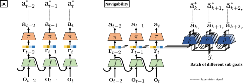
Figure 3: Learning navigability: the difference between classical behavior cloning (Left), which directly learns the main target policy $\pi$ on a downstream task, and learning navigability (Right), i.e. learning a representation $\mathbf{r}_{t}$ predicted by $f$ through a blind auxiliary policy $\rho$ allowing to navigate by predicting sequences of actions for a batch of different subgoals for each time instant $t$. The representation is then used by the downstream policy $\pi$.

We train the policy $\rho$ and the function $f$ predicting the representation $\mathbf{r}_{t}$ jointly by BC minimizing the error between actions $\bar{\mathbf{a}}_{k,j}$ and the GT actions $\bar{\mathbf{a}}^{*}_{k,j}$ derived from shortest path calculations:

$$\hat{f}= \textstyle{\arg\min_{f,\rho}\ \sum_{k}\sum_{j=1}^{B}\mathcal{L}_{CE}(\bar{\mathbf{a}}_{k,j},\bar{\mathbf{a}}^{*}_{k,j}),}$$ (5)

where $\mathcal{L}_{CE}$ is the cross-entropy loss and the index $k$ runs over all steps in the training set. Let us recall again a detail, which might be slightly hidden in the notation in equation (5): while the loss runs over the steps $k$ in short-trajectories, these steps are attached to the steps $t$ in long episodes through the visual representation $\mathbf{r}_{t}$ built by the encoder $f$, as in eq. (4). The auxiliary policy $\rho$ is a pre-text task and not used after training. Navigation is performed by the main agent $\pi$, which is finetuned on its own downstream objective.

Navigability vs. BC — there is a crucial difference to classical Behavior Cloning, which trains the main policy jointly with the representation $f$ from expert trajectories mimicking or approximating the desired optimal policy (see Ramrakhya et al. (2023) for comparisons), i.e.:

$$\mathbf{r}_{t} =f(\mathbf{o}_{t},\mathbf{r}_{t-1},\mathbf{a}_{t-1}),$$ (6)

$$p(\mathbf{a}_{t}) =\pi(\mathbf{r}_{t},G)$$ (7)

$$(\hat{f},\hat{\pi}) =\textstyle{\arg\min_{f,\pi}\sum_{i\in\mathcal{D}}\mathcal{L}_{CE}(\mathbf{a}_{i}^{*},\pi(\mathbf{r}_{i},g_{i})),}$$ (8)

where $G$ is the (global) navigation goal and $\mathcal{D}$ the training data. In the case of navigation, these experts are often shortest path calculations or human controllers combined with goal selection through hindsight. It is a well-known that BC is suboptimal for several reasons (Kumar et al., 2022). Amongst others, it depends on sufficient sampling of the state space in training trajectories, and it fails to adequately learn exploration in the case where no single optimal solution is available to the agent due to partial observability. In contrast, our navigability loss trains the representation $\mathbf{r}_{t}$ only, and can be combined with independently chosen downstream policies.

Subgoal mining — For a given compute budget, the question arises how many steps are spent on long vs. short episodes, as each step spent on a short episode is removing one visual observation from training — $\rho$ is blind. We sample waypoints on each long episode and attach a fixed number of subgoals to each waypoint sampled uniformly at a given Euclidean distance. Mining subgoal positions is key to the success of the method: Sampled too close, they lack information. Outside of the observed are (and thus not represented in $\mathbf{r}_{t}$), the blind auxiliary agent would have to rely on regularities in environment layouts to navigate, and not on $\mathbf{r}_{t}$. We sample a large initial number of subgoals and remove less informative ones, ie. those whose geodesic distance $d_{G}$ to the waypoint is close to its Euclidean distance $d_{E}$, i.e. $\frac{d_{G}}{d_{E}}{<}T$. For these, following the compass vector would be a sufficient strategy, non-informative about the visual representation. Details are given in Section 5.

Implementation and downstream tasks — Akin to training with PPO (Schulman et al., 2017), a rollout buffer is collected with multiple parallel environment interactions, on which the Navigability loss is trained. This facilitates optional batching of PPO with navigability, with both losses being separated over different environments — see Section 5, and the appendix for implementation.

Training of the agent is done in two phases: a first representation training, in which the main policy $\pi$, the representation $\mathbf{r}_{t}$ and the auxiliary agent $\rho$ are jointly trained minimizing $\mathcal{L}_{Nav}$, eq. (5). This is followed by fine-tuning on the downstream task with PPO. We also propose a combination of Navigability and BC losses using $\mathcal{L}=\mathcal{L}_{Nav}+\mathcal{L}_{BC}$. The advantages are two-fold: (i) training the main policy is not idle for environments selected for the Navigability loss, and (ii) visual observations gathered in environment steps spent in short episodes are not wasted, as they are used for training $\mathbf{r}_{t}$ through backpropagation through the main policy — see Section 5.

4 On the importance of the blindness property

We argue that blindness of the auxiliary agent is an essential property, which we motivate by considering the impact of the supervised learning objective in terms of compression and vanishing gradients.

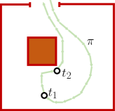
Figure 4: Beh. cloning.

Figure 4 shows a main agent $\pi$ which, after having entered the scene and made a circular motion, has observed the central square-shaped obstacle and the presence of the door it came through. Our goal is to maximize the amount of information on the obstacles and navigable space extracted by the agent through its training objective. Without loss of generality we single out the representation estimated at $t{=}t_{1}$ indicated in Figure 4. While this information is in principle present in the observation history $\{\mathbf{o}_{t}\}_{t\leq t_{1}}$, there is no guarantee that it will be kept in the representation $\mathbf{r}_{t}$ at $t{=}t_{1}$, as the amount of information storable in the recurrent memory $\mathbf{r}_{t}$ is much lower than the information observed during the episode. Agent training leads to a learned compression mechanism, where the policy (expressed through eq. (6) and (7)) compresses $\{\mathbf{o}_{t}\}_{t\leq t_{1}}$ in two steps: (1) information from $\mathbf{o}_{t}$ not useful at all is discarded by $f$ before it is integrated into $\mathbf{r_{t}}$; (2) information from $\mathbf{o}_{t}$ useful for a single step is integrated into $\mathbf{r}_{t}$, used by $\pi$ and then discarded by $f$ at the next update, i.e. it does not make it into $\mathbf{r}_{t+1}$. Here we mean by “information content” the mutual information (MI) between $\mathbf{r_{t}}$ and the observation history, i.e.

$$I(\mathbf{r}_{t};\mathbf{o}_{past})=\mathbb{E}_{p(\mathbf{o}_{past})}\left[\log\frac{p(\mathbf{r}_{t}|\mathbf{o}_{past})}{p(\mathbf{r}_{t})}\right],$$ (9)

where $\mathbf{o}_{past}=\{\mathbf{o}_{t^{\prime}}\}_{t^{\prime}\leq t}$. Dong et al. (2020) provide a detailed analysis of information retention and compression in RNNs in terms of MI and the information bottleneck criterion (Bialek et al., 2001).

The question therefore arises, whether the BC objective is sufficient to retain information on the scene structure observed before $t{=}t_{1}$ in $\mathbf{r}_{t}$ at $t{=}t_{1}$. Without loss of generality, let us single out the learning signal at $t{=}t_{2}$, where $t_{2}>t_{1}$, as in Figure 4. We assume the agent predicts an action $\mathbf{a}_{t}$, which would lead to a collision with the central obstacle, and receives a supervision GT signal $\mathbf{a}^{*}_{t}$, which avoids the collision: . Minimizing $\mathcal{L}(\mathbf{a}_{t},\mathbf{a}^{*}_{t})$ requires learning to predict the correct action $\mathbf{a}^{*}_{t}$ given its “input” $\mathbf{r}_{t}$, and in this case this can happen in two different reasoning modes:

(r1)

learning a memory-less policy which avoids obstacles visible in its current observation, or

(r2)

learning a policy which avoids obstacles it detects in its internal latent map, which was integrated over its history of observations.

It is needless to say that (r2) is the desired behavior compatible with our goal stated above. However, if minimizing the BC objective can be realized by both, (r1) and (r2), we argue that training will prioritize learning (r1) and neglect (r2) for essentially two reasons: firstly, the compression mechanism favors (r1) which does not require holding it in an internal state for longer than one step. Secondly, reasoning (r2) happens over multiple hops and requires backpropagation over multiple time instants, necessary for the integration of the observed sequence into a usable latent map. The vanishing gradient problem will make learning (r2) harder than the short chain reasoning (r1).

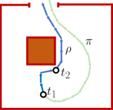
Figure 5: Navigability.

Let’s now consider the navigability loss, illustrated in Figure 5. The main agent $\pi$ integrates visual observations over its own trajectory up to waypoint $t{=}t_{1}$. The aux agent $\rho$ navigates on the blue trajectory and we again consider the effect of the supervised learning signal at $t{=}t_{2}$. Minimizing $\mathcal{L}(\mathbf{a}_{t},\mathbf{a}^{*}_{t})$ requires learning an agent which can predict the correct action $\mathbf{a}^{*}_{t}$ given its “input” $\mathbf{r}_{t}$, but now, this can happen in one way only: since the agent $\rho$ is blind, the BC objective cannot lead to reasoning (r1), i.e. memory-less, as it lacks the necessary visual observation to do so. To consistently predict the correct action $\mathbf{a}^{*}_{t}$, the representation $\mathbf{r}_{t}$ collected at $t{=}t_{1}$ is necessary, i.e. (r2). Making the aux agent blind has thus the double effect of resisting the compression mechanism in learning, and to force the learning signal through a longer backpropagation chain, both of which help integrating relevant observations into the agent memory. Ribeiro et al. (2020) have recently shown that information retention and vanishing gradients, albeit different concepts, are related.

For these reasons, navigability is different from data augmentation (DA): the steps on short episodes improve the representation integrated over visual observations on long episodes, whereas classical DA would generate new samples and train them with the same loss. We see it as generating a new learning signal for existing samples on long episodes using privileged information from the simulator.

An argument could be made that our stated objective, i.e. to force an agent to learn a latent map, is not necessary if optimizing BC does not naturally lead to it. As counter argument we claim that integrating visual information over time (r2) increases robustness compared to taking decisions from individual observations (r1), in particular in the presence of sim2real gaps. We believe that reactive reasoning (r1) will lead to more likely exploitation of spurious correlations in simulation then mapping (r2), and we will provide evidence for this claim in the sim2real experiments in Section 5.

Related work — recent work (Wijmans et al., 2023) has covered experiments on representations learned by a blind agent. Compared to our work, Wijmans et al. (2023) present an interesting set of experiments on the reasoning of a trained blind agent, but it does not propose a new method: no gradients flow from the probed agent to the blind one. In contrast, in our work the blind agent contributes to enrich the representation of a new navigation agent. Our situation corresponds to a non-blind person which is blind-folded and needs to use the previously observed information from memory, with gradients flowing back from the blindfolded situation to the non-blind one.

5 Experimental Results

We train all agents in the Habitat simulator (Savva et al., 2019) and the Gibson dataset (Xia et al., 2018). We follow the standard train/val split over scenes, i.e. $72$ training, $14$ for validation, $14$ for testing, with $\sim 68$k, $75$k and $71$k episodes per scene, respectively.

Subgoals — All standard episodes are used as long episodes during training, short episodes have been sampled additionally from the training scenes. To be comparable, evaluations are performed on the standard (long) episodes only. To produce short episodes, we sample waypoints every 3m on each long episode and attach 20 subgoals to each waypoint at a Euclidean distance $\in[3,5]$m. The threshold for removing uninformative subgoals is set to $T{=}1.5$m. This leads to the creation of $\sim 36$M short training episodes — no short episode is used for validation or testing.

Sim2Real — evaluating sim2real transfer is inherently difficult, as it would optimally require to evaluate all agent variants and ablations on a real physical robot and on a high number of episodes. We opted for a three-way strategy: (i) experiments evaluate the model and policy $\pi$ trained in simulation on a real physical robot. It is the only form of evaluation which correctly estimates navigation performance in a real world scenario, but for practical reasons we limit it to a restricted number of 11 episodes in a large (unseen) office environment shown in Fig. 1; (ii) Evaluation in allows large-scale evaluation on a large number of unseen environments and episodes; (iii) allows similar large-scale evaluation and approximates the transfer gap through artificial noise on simulation parameters. We added noise of different types, similar to Anderson et al. (2018), but with slightly different settings: Gaussian Noise of intensity 0.1 on RGB, Redwood noise with D=30 on depth, and actuator noise with intensity 0.5. Details are given in the appendix.

Metrics — we report Success, which is the number of correctly terminated episodes, and SPL (Anderson et al., 2018), which is Success weighted by the optimality of the navigated path, $\textit{SPL}=\frac{1}{N}\sum_{i=1}^{N}S_{i}\left(\frac{\ell_{i}^{*}}{\max(\ell_{i},\ell_{i}^{*})}\right),$ where $\ell_{i}$ is the length of the agent path in episode $i$ and $\ell_{i}^{*}$ is the length of the GT path. For the robot experiments we also consider Soft-SPL (Anderson et al., 2018), which extends SPL by changing the definition of $S_{i}$: in failed episodes it is weighted by the distance achieved towards the goal instead of being set to zero.

Training setup — we propose a 2-phase strategy with a fixed compute budget of $100$M env. steps:

Phase 1: Pre-training

takes $50$M steps. We combine and test 4 strategies: standard PPO, standard BC, Navigability loss and a reconstruction loss (details below), for a total of 8 variants (Table 1).

Phase 2: Fine-tuning

is the same for all methods, done with PPO (Schulman et al., 2017) for $50$M steps on the downstream PointGoal task. We reinitialize the main policy $\pi$ from scratch to evaluate the quality of the learned representation, the aux agent is not used. We use a common reward definition (Chattopadhyay et al., 2021) as $r_{t}=\mathrm{R}\cdot\mathbb{I}_{\text{success }}-\Delta_{t}^{\mathrm{Geo}}-\lambda$, where $R{=}2.5$, $\Delta_{t}^{\mathrm{Geo}}$ is the gain in geodesic distance to the goal, and a slack cost $\lambda{=}0.01$ encourages efficiency.

The best checkpoint is chosen on the validation set and all results are reported on the test set.

Table 1: Influence of the navigability loss and short episodes: we compare PPO (Schulman et al., 2017), BC=Behavior cloning and our Navigability, which constitute a Phase 1 of 50M env steps. 12 environments are trained in parallel, distributed over the different learning signals. In Phase 2, all of these methods are finetuned with PPO only for an additional 50M env steps. The best validation checkpoints of phase 2 are chosen and evaluated on the test set. ”Do \raisebox{-.9pt}{\small~S}⃝” = short episodes are used by the agent. \raisebox{-.9pt}{\small~L}⃝=long episodes, \raisebox{-.9pt}{\small~S}⃝=short episodes. The agent trained with navigability only has seen only 5% of the visual observations (=2.5M).

Table 2: Sim2Real transfer — Avg. performance over 11 episodes with a Locobot in a real environment (Fig. 1) using the Map+Plan baseline and agents trained with PPO, BC and ours, corresponding to variants (a,c,e) of Table 1.

Method	Success	SPL	sSPL
(-) Map+Plan	36.4	29.6	32.7
(a) PPO	45.5	14.7	20.0
(c) BC	72.7	36.3	36.3
(e) Navig. + BC	81.8	45.6	44.0

Robot experiments — are reported in Table 2 for three end-to-end trained agents (PPO, BC and our proposed agent) and for a map+plan method introduced by Gupta et al. (2017) and reused in (Chaplot et al., 2020b; a). A detailed description of the agents can be found further below. Overall, the differences in performance are significant, with a clear advantage of the proposed Navigability representation in terms of all 3 metrics, providing evidence for its superior robustness (Success) and efficiency (SPL, sSPL). Qualitatively, the three agents show significantly different behavior on these real robot experiments. Our Navigability+BC variant is more efficient in reaching the goals and goes there more directly. The PPO agent shows zig-zag motion (increasing SPL and sSPL), and, in particular, often requires turning, whose objective we conjecture is to orient and localize itself better. The BC variant struggled less with zig-zag motion but created significantly longer and more inefficient trajectories than the proposed Navigability agent.

Impact of navigability — is studied in Table 1, which compares different choices of pre-training in phase 1. For each experiment, agents were trained on 12 parallel environments. These environments where either fully used for training with BC (with a choice of the proposed navigability loss or classical BC of the main policy, or both), or fully used for classical RL with PPO training with PointGoal reward, or mixed (6 for BC and 6 for PPO), indicated in columns Nr. Envs PPO and Nr. BC Envs, respectively. Agents trained on the navigability loss navigated fewer steps over the long episodes and saw fewer visual observations, only 5% = 2.5M. We see that PPO (a) outperforms classical BC (b), which corroborates known findings in the literature. The navigability loss alone (d) is competitive and comparable, and outperforms these baselines when transferred to noisy environments. Mixing training with PPO on the PointGoal downstream task in half of the training environments, as done in variants (f) and (g), does not provide gains.

Table 3: Impact of the hidden state of the main policy $\pi$ at transitions between long and short episodes: (c.1) set to zero (short episodes are data augme.); (c.2) set to last waypoint (clear separation of short and long ep.); (c.3) always continue (maximize episode length but introduce sparse teleportations).

Method	Eval Sim		Eval NoisySim
	Succ	SPL	Succ	SPL
(c.1) Set to zero	90.3	74.5	85.1	64.8
(c.2) Set to last waypoint	88.6	74.2	81.4	63.0
(c.3) Always continue	94.2	80.1	89.6	74.0

Table 4: Communicating with the Mole: Impact of the choice of connection between representation $r$ and blind policy $\rho$ for agent (e) of Table 1. (e.1) $\mathbf{r}_{t}$ is fed as “observed” input to $\rho$ at each step; (e.2) as initialization of $\rho$’s own hidden state; (e.3) as previous, but 128 additional dimensions are added to the state of $\rho$.

Method		Eval Sim		Eval NoisySim
	$|\mathbf{h}|$	Success	SPL	Success	SPL
(e.1) As observation	512	92.8	77.4	90.9	73.3
(e.2) Copy	512	95.5	80.3	80.7	62.5
(e.3) Copy+extend	640	90.4	76.9	83.3	66.6

Optimizing usage of training data — As the number of environment steps is constant over all agent variants evaluated in Table 1, the advantage of the Navigability loss in terms of transferability is slightly counter-balanced by a disadvantage in data usage: adding the short episodes to the training in variant (d) has two effects: (i) a decrease in the overall length of episodes and therefore of observed information available to agents; (ii) short episodes are only processed by the blind agent, and this decreases the amount of visual observations available to $\sim$5%. Combining Navigability with classical BC in agent (e) in Table 1 provides the best performance by a large margin. This corroborates the intuition expressed in Section 3 of the better data exploitation of the hybrid variant.

Is navigability reduced to data augmentation? — a control experiment tests whether the gains in performance are obtained by the navigability loss, or by the contribution of additional training data in the form of short episodes, and we again recall, that the number of environment steps is constant over all experiments. Agent (c) performs classical BC on the same data, i.e. long and short episodes. It is outperformed by Navigability combined with BC, in particular when subject to the sim2noisy-sim gap, which confirms our intuition of the better transferability of the Navigability representation.

Continuity of the hidden state — The main agent $\pi$ maintains a hidden state $\mathbf{r}_{t}$, updated from its previous hidden state $\mathbf{r}_{t-1}$ and the current observation $\mathbf{o}_{t}$. If this representation is a latent map, then, similar to a classical SLAM algorithm, the state update needs to take into account the agent dynamics to perform a prediction step combined with the integration of the observation. When the agent is trained through BC of the main agent on long and short episodes, as for variants (c) and (e), the main agent follows a given long episode and it is interrupted by short episodes. How should $\mathbf{r}_{t}$ be updated when the agent “teleports” from the terminal state of a short episode back to the waypoint on the long trajectory? In Table 4 we explore several variants: setting $\mathbf{r}_{t}$ to zero at waypoints is a clean solution but decreases the effective length of the history of observations seen by the agent. Saving $\mathbf{r}_{t}$ at waypoints and restoring it after each short episode ensures continuity and keeps the amount of observed scene intact. We lastly explore a variant where the hidden state always continues, maximizing observed information, but leading to discontinuities as the agent is teleported to new locations. Interestingly, this variant performs best, which indicates that data is extremely important. Note that during evaluation, only long episodes are used and no discontinuities are encountered.

Communication with the Mole — in Table 4 we explore different ways of communicating the representation $\mathbf{r}_{t}$ from the main to the aux policy during Phase 1. In variant (e.1), $\rho$ receives $\mathbf{r}_{t}$ as input at each step; in variants (e.2) and (e.3), the hidden GRU state $\mathbf{h}$ of $\rho$ is initialized as $\mathbf{r}_{t}$ at the beginning of each short episode, and no observation (other than the subgoal $g_{.}$) is passed to it. Variant (e.2) is the best performing in simulation, and we conjecture that this indicates a likely ego-centric nature of the latent visual representation $\mathbf{r}_{t}$. Providing it as initialization allows it to evolve and be updated by the blind agent during navigation. This is further corroborated by the drop in performance of these variants in NoisySim, as the update of an ego-centry representation requires odometry, disturbed by noise in the evaluation, and unobserved during training. Adding 128 dimensions to the blind agent hidden state $\mathbf{h}$ in variant (e.3) does not seem to have an impact.

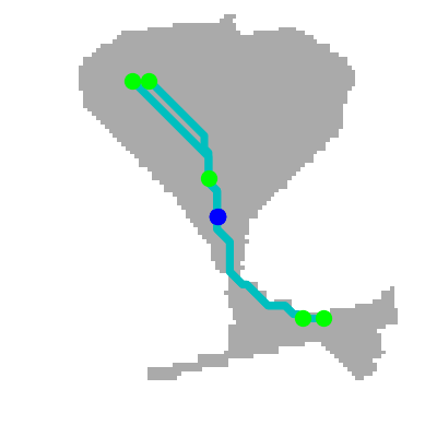
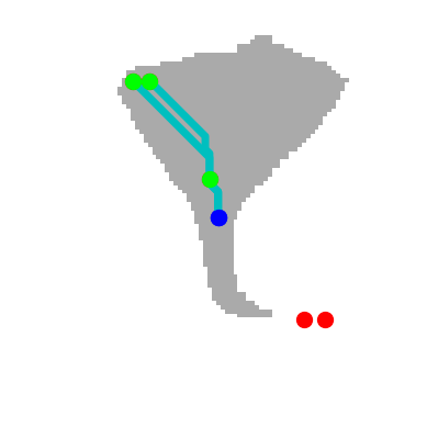
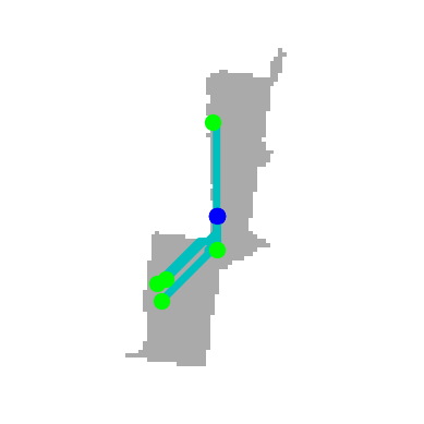
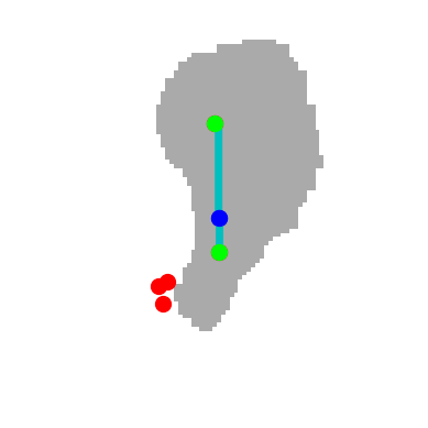
GT	(a) PPO	GT	(c.1) BC
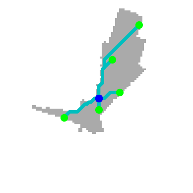
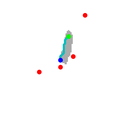
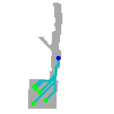
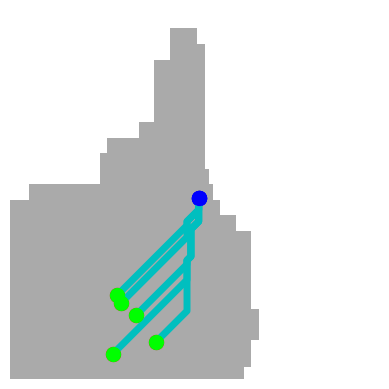
GT	(c.3) BC	GT	(e) Ours

	Sim			NoisySim
Method	Reconstr.	2D Nav.		Reconstr.	2D Nav.
	IoU	Succ.	Sym-SPL	IoU	Succ.	Sym-SPL
(a) PPO	31.0	37.9	10.1	15.8	18.4	6.1
(c.1) BC\raisebox{-.9pt}{\small~L}⃝\raisebox{-.9pt}{\small~S}⃝	25.5	45.2	11.0	11.1	16.2	4.6
(c.3) BC\raisebox{-.9pt}{\small~L}⃝\raisebox{-.9pt}{\small~S}⃝	11.9	13.2	3.5	1.1	0.6	0.3
(e) Navig.+BC	19.8	66.5	14.7	18.0	64.8	13.2
Viewpoints on figures on the left are not comparable as different agents perform different trajectories. The agent is the blue dot in the center and 5 trajectories out of 10 used for Sym-SPL are plotted. Goal points are green when reachable (always in GT) and red otherwise.

Figure 6: Probing reconstruction: we evaluate how much information on reconstruction is contained in the learned representations. PPO (a) is able to capture well only parts of the map, leading to navigation failures. Reconstruction by (c.1) exhibits similar characteristics. The (c.3) variant performs poorly according to all metrics, and the reconstructed map confirms that. Our approach, (e), estimates less accurately than PPO and (c.1) the shape of the navigable space, but captures well the geometry of the environment.

Probing the representations — of a blind agent has been previously proposed by Wijmans (2022); Wijmans et al. (2023). We extend the procedure: for each agent, a dataset of pairs $\{(\mathbf{r}_{i},\mathbf{M}^{*}_{i})\}_{i=1..D}$ is generated by sampling rollouts. Here, $\mathbf{r}_{i}$ is the hidden GRU state and $\mathbf{M}^{*}_{i}$ is an ego-centric 2D metric GT map of size $95{\times}95$ calculated from the simulator using only information observed by the agent. A probe $\phi$ is trained on training scenes to predict $\mathbf{M}_{i}=\phi(\mathbf{r}_{i})$ minimizing cross-entropy, and tested on val scenes. Results and example reconstructions on test scenes are shown in Fig. 6. We report reconstruction performance measured by IoU on unseen test scenes for variants (a), (c) and (e), with (c) declined into sub-variants (c.1) and (c.3) from Table 4. PPO outperforms the other variants on pure reconstruction performance in the noiseless setting, but this is not necessarily the goal of an actionable representation. We propose a new goal-oriented metric directly measuring the usefulness of the representation in terms of navigation. For each pair $(\mathbf{M}_{i},\mathbf{M}^{*}_{i})$ of predicted and GT maps, we sample $N{=}10$ reachable points $\{p_{n}\}_{n=1..N}$ on the GT map $\mathbf{M}^{*}_{i}$. We compute two shortest paths from the agent position to $p_{n}$: one on the GT map $\mathbf{M}^{*}_{i}$, $\ell_{i,n}^{*}$, and one on the predicted map $\mathbf{M}_{i}$, $\ell_{i,n}$. We introduce Symmetric-SPL as $\textit{Sym-SPL}=\sum_{i=1}^{D}\sum_{n=1}^{N}S_{i,n}\min\left(\frac{\ell_{i,n}}{\ell_{i,n}^{*}},\frac{\ell_{i,n}^{*}}{\ell_{i,n}}\right)$, where, similar to SPL, $S_{i,n}$ denotes success of the episode, but on the predicted map $\mathbf{M}_{i}$ and towards $p_{n}$. Results in the table associated with Figure 6 show that the representation learned with the Navigability loss leads to better navigation performance, in particular in NoisySim, corroborating our claim of transferability.

Table 5: Map+plan baseline.

Method	Noise	Succ.	SPL
Class.	no	95.7	89.9
Ours (e)	no	95.5	80.3
Class.	yes	27.9	16.3
Ours (e)	yes	90.9	73.3

Further comparison with reconstruction — we claim that unnecessarily accurate reconstruction is sub-optimal in presence of high sim2real gap, and, additional to already discussed , we compare in simulation with a method supervising reconstruction. The loss is identical to the probing loss described above, but used to train the representation during Phase 1, combined with BC. Corresponding method (h) in Table 1 compares unfavorably with our method (e), in particular in . In Table 5 we also compare with a classical map+plan baseline of Gupta et al. (2017) and show that under noisy conditions our approach outperforms the classical planner.

6 Conclusion

Inspired by Cognitive Maps in biological agents, we have introduced a new technique, which learns a latent representations from interactions of a blind agent with the environment. We position it between explicit reconstruction, arguably not the desired when a high sim2real gap is present, and pure end-to-end training on a downstream task, which is widely argued to provide a weak learning signal. In experiments on sim2real and sim2noisy-sim evaluations, we have shown that our learned representation is particularly robust to domain shifts.

Appendix A Appendix

A.1 Comparison with SOTA

Comparisons are difficult, as no clear evaluation protocol exists, in particular when transfer and sim2real performance is targeted. In Table 6 we attempt to provide a non-exhaustive review of PointGoal performance targeting transfer situations particularly. However, we need to point out that the performance numbers are not comparable, as there are very large variations in setups, training regimes, data, number of test episodes etc.

A.2 Architecture of the agents

An architecture diagram of the full agent is given in Figure 7. The main agent $\pi$ uses a standard architecture from the literature, eg. in (Wijmans et al., 2019) and a large body of follow-up work. A half-width, $4$-channels ResNet18 encodes the RGB-D frames into a $512$D vector. A linear layer encodes the pointgoal information with integrated GPS and compass as a $64$D vector. An embedding layer (a trained LUT) encodes the previous action into a $32$D vector. These 3 vectors are then concatenated to form the input of a GRU, which updates the $512$D vector representing the internal state of the agent after each new observation. The internal state is finally fed to 2 linear layers to compute the log-probabilities of each action and an estimate of the current state value, respectively.

Method	Steps	Setup	Eval Sim		Eval NoisySim		Eval Real
			Success	SPL	Success	SPL	Success	SPL
DDPO (Wijmans et al., 2019)	2.5G	Gibson-2+, SE-ResNetXt101 + 1024-d LSTM	98.0	94.8	N/A	N/A	N/A	N/A
	2.5G	Gibson-2+, ResNet50 + LSTM-512	-	94.0	N/A	N/A	N/A	N/A
EmbVizNav(Rosano et al., 2021)	2.5G+2.4M	Gibson+MP3D+real obs., eval on custom scene, RGB only	99.1	91.3	N/A	N/A	97.0	80.0
VizOdomNav(Partsey & Maksymets, 2021)	2M	Gibson (Hab. Challenge 2021)	86.0	66.0	N/A	N/A	N/A	N/A
Robust-Nav (Chattopadhyay et al., 2021)	75M+166k	Exhaustive evaluation in sim2noisy-sim	Check paper for a broad study w. multiple params
Sadek et al. (Sadek et al., 2022)	100M	Real robot, 20 eval episodes only, avg of 2 custom environm.	86.4	71.1	N/A	N/A	75.0	53.9
S2R Pred (Kadian et al., 2020)	500M	Training w. sliding on, no train noise	N/A	36.0	N/A	N/A	N/A	61.0
	500M	Training w/o sliding, Training noise	N/A	36.0	N/A	N/A	N/A	61.0
Ours	100M	Hybrid Navigability+BC followed by PPO, no train noise	95.5	80.3	90.9	73.3	81.8	45.6

Table 6: Comparison with SOTA — These numbers are not comparable as no clear experimental protocol exists for sim2real or sim2noisy-sim experiments. The reported experiments feature extreme variations in setups, training regimes, data, number of test episodes. Several papers report a large number of experiments, we reproduce only a small number of variants here. Agent Ours is agent (e) in Table 1.

When a waypoint is reached along the main path, the main agent stores its internal state (see Section A.5 for implementation details of the training algorithm). The auxiliary agent $\rho$ (a.k.a. the “mole”) starts exploring subgoals from the waypoint. Its inputs are the internal state of the main agent when it reached the waypoint, a new “sub-pointgoal” vector pointing towards the currently pursued subgoal, the previously taken action, and its own auxiliary internal state. The “sub-pointgoal” and the previous action are encoded through similar linear and embedding layers as the main agent, respectively. It also has its own GRU, followed by a linear layer producing the action log-probabilities.

As described in the main text and ablated in Table 4 , we tested a few different ways to connect the internal state of the main agent to the auxiliary one: 1. Concatenate it with the other features before feeding it as an input to the auxiliary GRU; 2. Use it to initialize the auxiliary internal state; 3. Use it to initialize part of the auxiliary internal state while keeping some room for values dedicated to the subgoal exploration task.

Figure 7: Architecture of the encoder $f$, the main agent $\pi$ and the auxiliary agent $\rho$

A.3 Probing experiments

A.3.1 Architecture of the probing agent

The probing network’s architecture is inspired by the approach proposed in (Wijmans, 2022; Wijmans et al., 2023). It processes the $512$D vector $\mathbf{r}_{i}$, representing the GRU memory after pre-training (Phase 1 in Section 5) with a 2-layer MLP with $256$ hidden dimensions to produce an output vector of dimension $1600$. This vector is reshaped into a 3D tensor of size $[64,5,5]$ and processed by a Coordinate Convolution (CoordConv) layer (Liu et al., 2018), followed by four CoordConv-CoordUpConv (Coordinate Up-Convolution) blocks. Each such block is composed of:

2D Dropout layer

with dropout probability $0.05$;

CoordConv layer

with kernel size = 3, padding = 1, stride = 1, that reduces the channel size by half while keeping the other dimensions intact;

CoordUpConv layer

with kernel size = 3, padding = 0, stride = 2, that maintains the channel dimension and doubles the spatial dimensions of the feature map;

ReLU activation

, except for the last block where it is removed.

This stack produces a feature map of dimension $[4,95,95]$ that is processed by a $1\!\times\!1$-Convolution layer to create the output of size $[2,95,95]$, that represents the unnormalized logits of each map pixel being navigable and non-navigable.

For each agent tested, we create a training dataset by running the agent on a subset of 150 episodes for each of the 72 scenes of the Gibson PointGoal training split for a total of 10,800 episodes. We evenly sample each trajectory to obtain approximately 20 observations for each episode, so that we collect training sets of about 200,000 samples. Using the same procedure we also collect a validation dataset from 14 Gibson scenes comprising approximately 20,000 samples, and a test dataset built using the Gibson Pointgoal val split also comprising 20,000 samples.

The probing network is trained with a batch size of $64$ using the AdamW optimizer (Loshchilov & Hutter, 2018) with learning rate $10^{-3}$ and weight decay $10^{-5}$ to minimize the cross-entropy loss $\mathcal{L}_{CE}$ between groundtruth and reconstructed occupancy maps. The validation dataset is used to perform early-stopping, which in probing experiments is particularly important to avoid that scene structure gets its way into the parameters of the probing network.

A.3.2 Additional probing experiments

Method		GT	Pred.		GT	Pred.		GT	Pred.
(a) PPO
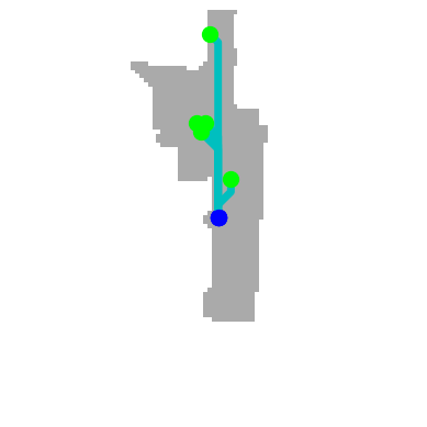
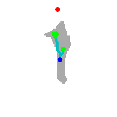
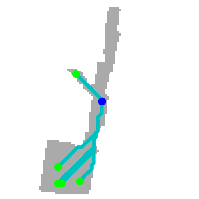
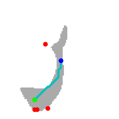
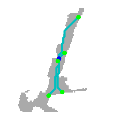
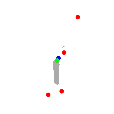
(c.1) BC
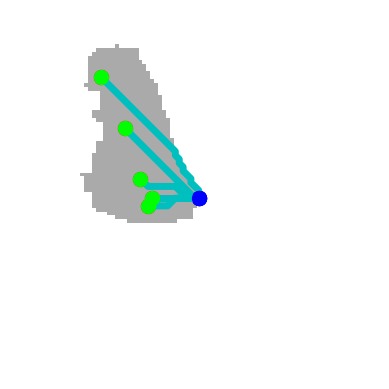
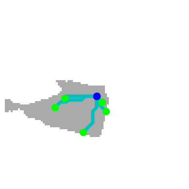
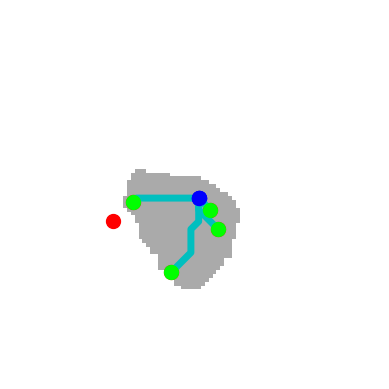
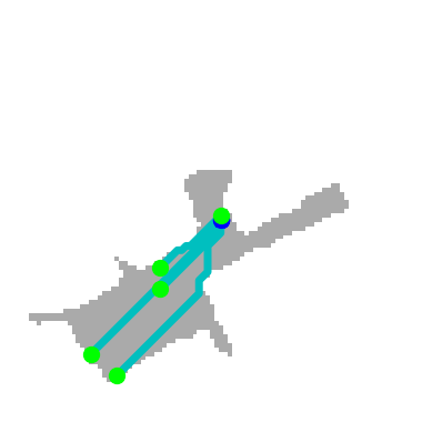
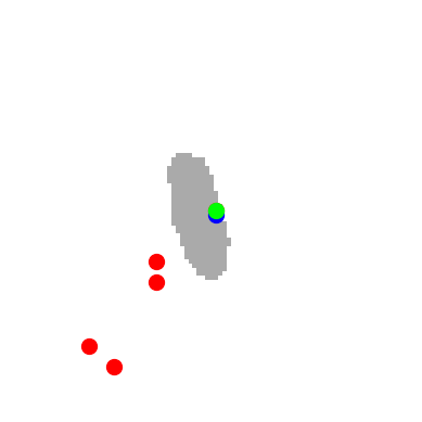
(c.3) BC
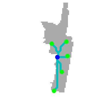
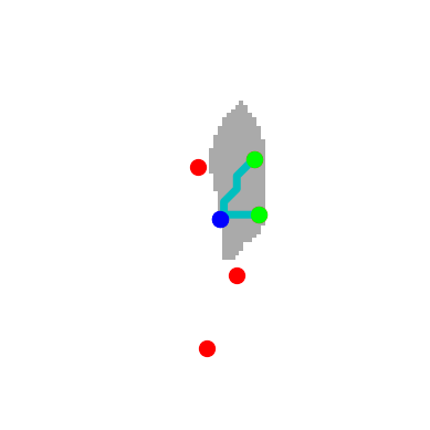
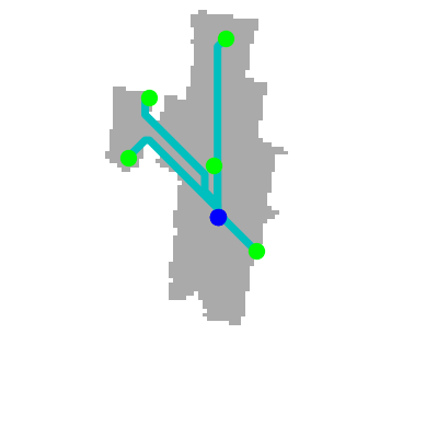
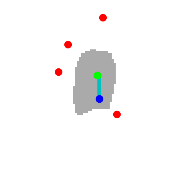
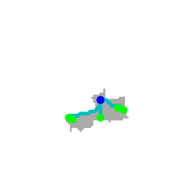
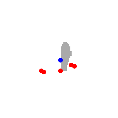
(e) Ours

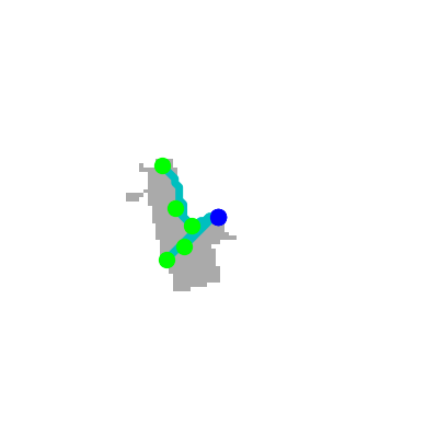
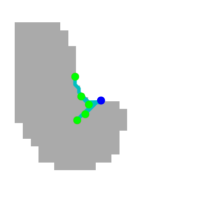
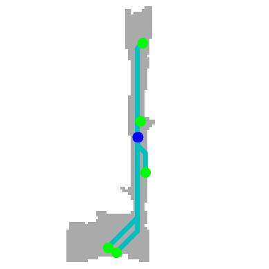
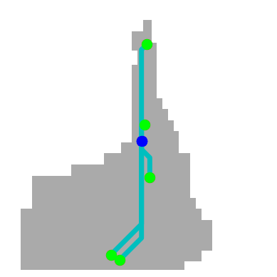
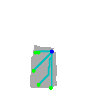
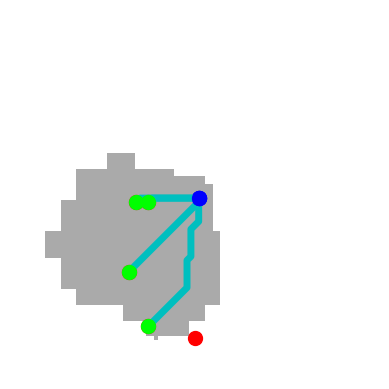
Figure 8: Additional probing results: Sim setting without noise. Three pairs of groundtruth and predicted navigable maps (in gray) for the four agents (a), (c.1), (c.3) and (e). The agent is in the center (blue dot), and 5 of the 10 trajectories used to compute the Symmetric-SPL are plotted with light blue lines. Trajectories terminate with green goal points when the target is reachable, while target points are red when not reachable, and no trajectory leads to them.

Method		GT	Pred.		GT	Pred.		GT	Pred.
(a) PPO
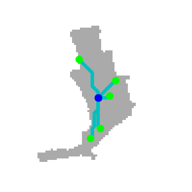
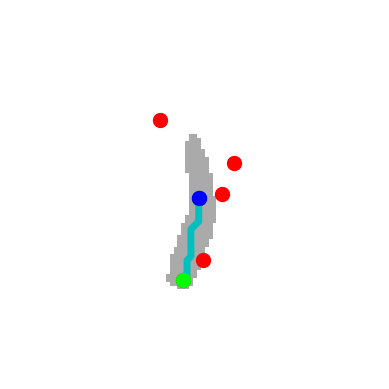
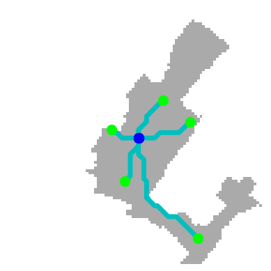
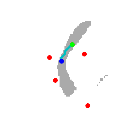
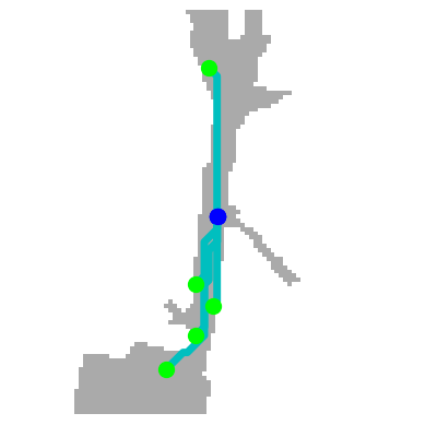
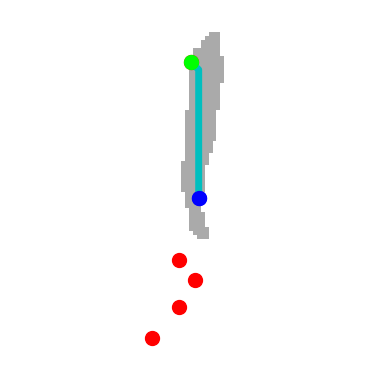
(c.1) BC
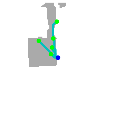
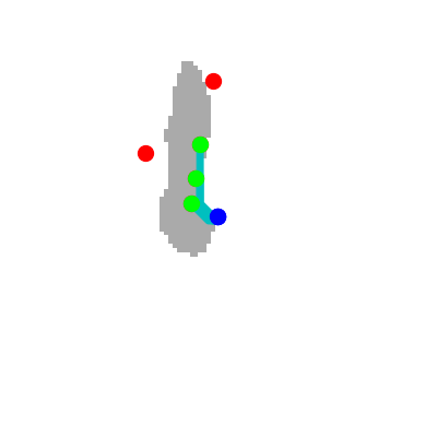
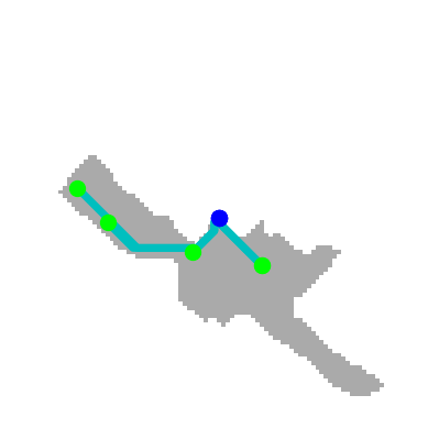
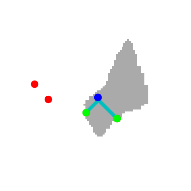
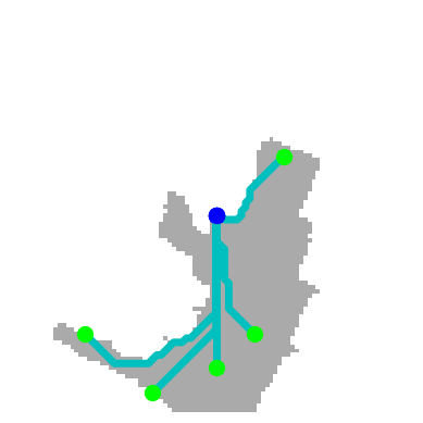
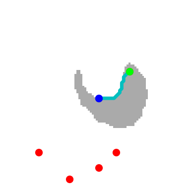
(c.3) BC
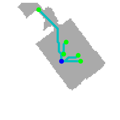
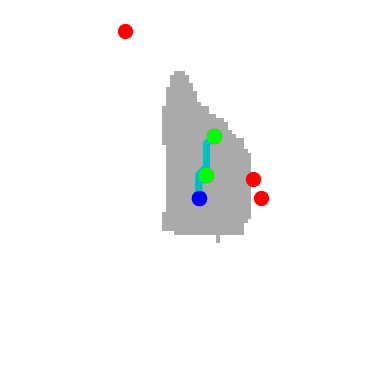
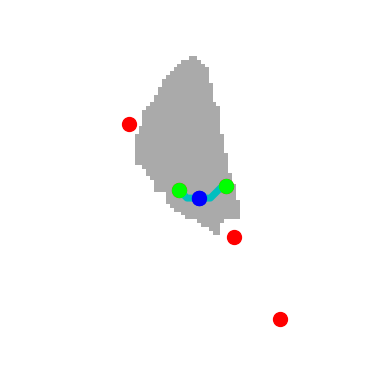
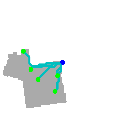
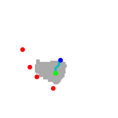
(e) Ours

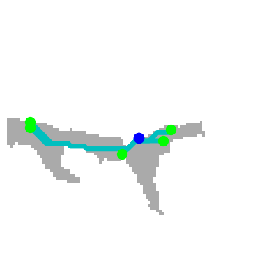
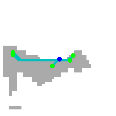
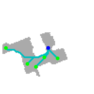
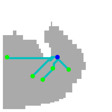
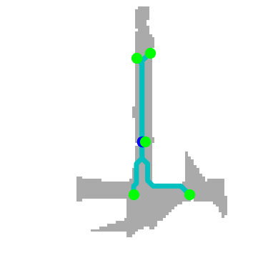
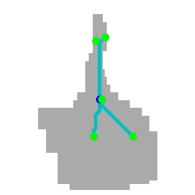
Figure 9: Additional probing results: NoisySim setting. Three pairs of groundtruth and predicted navigable maps with shortest path trajectories for agents (a), (c.1), (c.3) and (e).

As discussed in the main text, we visualize the probing results for four agent variants: (a), (c) and (e) from Table 1 and Table 2 from the main text, with (c) declined into sub-variants (c.1) and (c.3) in Table 4. The reconstructed maps are shown in Figures 8 and 9. As a reminder, (a) is a standard PPO agent, while (c) variants are trained using behaviour cloning.

Figure 8 shows examples of reconstructed occupancy maps for the four agents in the Sim environment without noise. PPO estimates reasonably well the shape of the navigable space, but it is somewhat conservative and captures well only parts of the map, leading to frequent navigation failures. Reconstructions provided by (c.1) exhibit similar characteristics. The (c.3) variant performs poorly according to all quantitative probing metrics, and the reconstructed maps visually confirm that. Teleportation seems to severely compromise the representation for the probing task. The proposed approach, agent (e), estimates less accurately than PPO and variant (c.1) the shape of the navigable space, but captures reasonably well the geometry of the environment, especially in the vicinity of the agent.

Figure 9 displays qualitative evaluations on the NoisySim environment. In this regime the proposed approach clearly outperforms alternative methods, producing predictions comparable to the noiseless setting, while other methods’ predictions degrade significantly. These results substantiate the claim that the representation learned in the pre-training phase with the proposed approach is more robust and transferable than those of alternative methods.

A.4 Details of the NoisySim eval environment

Complementary to our evaluation experiments on the real Locobot, our evaluation experiments in simulation were conducted in, both, not-noisy and noisy simulated environments. Our noisy environment is largely based on the noise settings of the CVPR Habitat challenge (Kadian et al., 2019), more specifically Gaussian noise on the RGB image, Redwood noise on the Depth image and Proportional Controller noise on the actuators.

However, we have applied some adjustments, motivated by the different objectives of our work, which is to transfer agents from simulation to the target domain with zero domain adaptation to evaluate the transferability of the learned representation. We have observed that in the Habitat implementation of the depth noise model, a depth $D$ above a given threshold $T$ was set to zero, i.e.

$$\texttt{if }( D>T)$$ (10)

$$D=0,$$

which is the inverse behavior of the noiseless setting, ie.

$$\texttt{if }( D>T)$$ (11)

$$D=T,$$

We argue that this extremely strong discrepancy does not fall into the category of noise but rather to a change in the nature of the sensor, messes up transfer and does not allow a sound evaluation — we therefore replaced (10) by the thresholding process of the standard variant (11).

Secondly, since the original Redwood noise was designed for $640\times 480$ images (Teichman et al., 2013), applying it to arbitrarily size depth image caused the appearance of black borders. We have extended this by setting depth on the borders to their original values.

A.5 Details on the implementation of Navigability

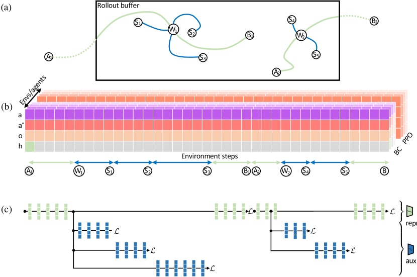
Figure 10: Illustration of the implementation of the navigability loss. (a) An example showing two long episodes, first going from $A_{1}$ to $B_{1}$, second from $A_{2}$ to $B_{2}$. Each episode has one waypoint each and several sub-goals and short episodes branching out from the waypoints. (b) As in PPO, learning is implemented with a rollout buffer, which stores a sub sequence. (c) The computation graph of an agent only trained on the navigability loss. The hidden state of the representation $f$ is collected on long episodes (Green) and the hidden state of auxiliary agent $\rho$ is collected on short episodes (Blue).

Figure 10 illustrates the implementation of the navigability loss in an example showing two long episodes, the first going from $A_{1}$ to $B_{1}$, the second from $A_{2}$ to $B_{2}$. Each episode has one waypoint each and several sub-goals and short episodes branching out from the waypoints, shown in Figure 10a. As in PPO, learning is implemented with a rollout buffer, which stores a sub sequence of the episode. The rollout buffer of length 128 steps in our implementation can hold one or several long sequences, or only a part of one or more sequences.

As mentioned in the paper, and as is custom in the literature, we train with multiple parallel environments. We strictly separate between two types of environments, and maintain separate rollout buffers for these two types:

PPO Environments

— are classical environments trained with RL (the PPO variant). As classically done, the rollout buffer is filled in the collection step and used for policy updates in the update step. No short sequences are used, and the trajectories are the ones taken by the agent.

BC Environments

— are either trained with classical behavior cloning (BC) or with our Navigability loss or with a combination of these two. In this case, as shown in Figure 10b, we flatten the hierarchical structure of long and short episodes into a single sequence, with the agent navigating between waypoints, at each waypoint going through the different short episodes, and then resuming at the waypoint again. The hidden state of the agent is stored at waypoints and restored if necessary, according to the choices ablated in Table 4.

Both types of environments are combined into a single unique batch for gradient updates.

Figure 10c illustrates how the rollout buffer of Figure 10b is mapped to the computation graph of the full agent combining the representation predictor $f$, main policy $\pi$ and the auxiliary policy $\rho$, when everything is trained with the navigability loss only. Vertical time instants of Figures 10a and 10b are aligned and correspond to each other. In its purest form, ie. agent variant (d) of Table 1, only the navigability loss is used for training. In this case, the hidden state of the representation $f$ is collected on long episodes (Green) and the hidden state of auxiliary agent $\rho$ is collected on short episodes (Blue).

A.6 Details on mapping predicted discrete actions to velocity Locobot actions

In the experiments involving simulation only, all actions were discrete, and as stated in the main paper, were taken from the alphabet $\{$MOVE_FORWARD 25cm, TURN_LEFT, TURN_RIGHT and STOP$\}$. The experiments on the real robot (the Locobot) required mapping the predictions of these discrete actions to velocity commands. A widely used closed-loop strategy executes each action by a closed-loop controller until the discrete action is terminated, then pauses to collect sensor readings, performs a prediction by the neural agent, and repeats. This strategy leads to slow executation and delays between discrete actions.

We have opted for a handcrafted 0-order hold, open-loop velocity command, which led to a speed-up of a factor of around 3$\times$-4$\times$. We map each discrete action to an equivalent velocity command $v$ to be sent to the Kobuki driver of the LoCoBot through ROS for execution. Then, we wait for a fixed waiting time $\Delta_{t}$ to collect the observations (RGB-D and pose). Here, $v$ is either linear velocity $v_{l}$ or angular velocity $v_{a}$ depending on the action taken. We empirically, found that setting $v_{l}$ to 0.25m/sec and $v_{a}$ to $\pm$ 60deg/sec for a fixed waiting ($\Delta_{t}$ = 2 seconds) was the best setup to execute the required discrete actions.

References

- Anderson et al. (2018) Peter Anderson, Angel X. Chang, Devendra Singh Chaplot, Alexey Dosovitskiy, Saurabh Gupta, Vladlen Koltun, Jana Kosecka, Jitendra Malik, Roozbeh Mottaghi, Manolis Savva, and Amir Roshan Zamir. On evaluation of embodied navigation agents. arXiv preprint, 2018.
- Andrychowicz et al. (2017) Marcin Andrychowicz, Filip Wolski, Alex Ray, Jonas Schneider, Rachel Fong, Peter Welinder, Bob McGrew, Josh Tobin, Pieter Abbeel, and Wojciech Zaremba. Hindsight Experience Replay. In NeurIPS, 2017.
- Banino et al. (2018) Andrea Banino, Caswell Barry, Benigno Uria, Charles Blundell, Timothy Lillicrap, Piotr Mirowski, Alexander Pritzel, Martin J Chadwick, Thomas Degris, Joseph Modayil, Greg Wayne, Hubert Soyer, Fabio Viola, Brian Zhang, Ross Goroshin, Neil Rabinowitz, Razvan Pascanu, Charlie Beattie, Stig Petersen, Amir Sadik, Stephen Gaffney, Helen King, Koray Kavukcuoglu, Demis Hassabis, Raia Hadsell, and Dharshan Kumaran. Vector-based navigation using grid-like representations in artificial agents. Nature, 557, 2018.
- Beeching et al. (2020a) Edward Beeching, Jilles Dibangoye, Olivier Simonin, and Christian Wolf. Learning to reason on uncertain topological maps. In ECCV, 2020a.
- Beeching et al. (2020b) Edward Beeching, Christian Wolf, Jilles Dibangoye, and Olivier Simonin. EgoMap: Projective mapping and structured egocentric memory for Deep RL. In ECML-PKDD, 2020b.
- Bialek et al. (2001) William Bialek, Ilya Nemenman, and Naftali Tishby. Predictability, Complexity, and Learning. Neural Computation, 13(11):2409–2463, November 2001.
- Blier et al. (2021) Léonard Blier, Corentin Tallec, and Yann Ollivier. Learning Successor States and Goal-Dependent Values: A Mathematical Viewpoint. In arXiv:2101.07123, 2021.
- Blodgett (1929) Hugh Carlton Blodgett. The effect of the introduction of reward upon the maze performance of rats. University of California Publications in Psychology, 4:133–134, 1929.
- Bresson et al. (2017) Guillaume Bresson, Zayed Alsayed, Li Yu, and Sébastien Glaser. Simultaneous localization and mapping: A survey of current trends in autonomous driving. IEEE Transactions on Intelligent Vehicles, 2017.
- Burgard et al. (1998) Wolfram Burgard, Armin B Cremers, Dieter Fox, Dirk Hähnel, Gerhard Lakemeyer, Dirk Schulz, Walter Steiner, and Sebastian Thrun. The interactive museum tour-guide robot. In Aaai/iaai, pp. 11–18, 1998.
- Chaplot et al. (2020a) Devendra Singh Chaplot, Dhiraj Gandhi, Abhinav Gupta, and Ruslan Salakhutdinov. Object goal navigation using goal-oriented semantic exploration. In In Neural Information Processing Systems, 2020a.
- Chaplot et al. (2020b) Devendra Singh Chaplot, Dhiraj Gandhi, Saurabh Gupta, Abhinav Gupta, and Ruslan Salakhutdinov. Learning to explore using active neural slam. In ICLR, 2020b.
- Chattopadhyay et al. (2021) Prithvijit Chattopadhyay, Judy Hoffman, Roozbeh Mottaghi, and Aniruddha Kembhavi. Robustnav: Towards benchmarking robustness in embodied navigation. CoRR, 2106.04531, 2021.
- Chebotar et al. (2021) Yevgen Chebotar, Karol Hausman, Yao Lu, Ted Xiao, Dmitry Kalashnikov, Jake Varley, Alex Irpan, Benjamin Eysenbach, Ryan Julian, Chelsea Finn, and Sergey Levine. Actionable Models: Unsupervised Offline Reinforcement Learning of Robotic Skills, 2021.
- Chen et al. (2021) Lili Chen, Kevin Lu, Aravind Rajeswaran, Kimin Lee, Aditya Grover, Michael Laskin, Pieter Abbeel, Aravind Srinivas, and Igor Mordatch. Decision transformer: Reinforcement learning via sequence modeling. In NeurIPS, 2021.
- Chen et al. (2022) Shizhe Chen, Pierre-Louis Guhur, Makarand Tapaswi, Cordelia Schmid, and Ivan Laptev. Think Global, Act Local: Dual-scale Graph Transformer for Vision-and-Language Navigation. arXiv:2202.11742, 2022.
- Cho et al. (2014) Kyunghyun Cho, Bart van Merriënboer, Caglar Gulcehre, Dzmitry Bahdanau, Fethi Bougares, Holger Schwenk, and Yoshua Bengio. Learning phrase representations using RNN encoder–decoder for statistical machine translation. In Conference on Empirical Methods in Natural Language Processing, 2014.
- Cueva & Wei (2018) Christopher J. Cueva and Xue-Xin Wei. Emergence of grid-like representations by training recurrent neural networks to perform spatial localization. In ICLR, 2018.
- Dashora et al. (2021) Nitish Dashora, Daniel Shin, Dhruv Shah, Henry Leopold, David Fan, Ali Agha-Mohammadi, Nicholas Rhinehart, and Sergey Levine. Hybrid imitative planning with geometric and predictive costs in off-road environments. In NeurIPS Workshop on Deep-RL, 2021.
- Dey et al. (2023) Sombit Dey, Assem Sadek, Gianluca Monaci, Boris Chidlovskii, and Christian Wolf. Learning whom to trust in navigation: dynamically switching between classical and neural planning. In IROS, 2023.
- Ding et al. (2019) Yiming Ding, Carlos Florensa, Pieter Abbeel, and Mariano Phielipp. Goal-conditioned imitation learning. In NeurIPS, 2019.
- Dong et al. (2020) Zhe Dong, Deniz Oktay, Ben Poole, and Alexander A. Alemi. On Predictive Information in RNNs, 2020.
- Du et al. (2021) Heming Du, Xin Yu, and Liang Zheng. VTNet: Visual Transformer Network for Object Goal Navigation. 2021.
- Eysenbach et al. (2021) Benjamin Eysenbach, Shreyas Chaudhari, Swapnil Asawa, Sergey Levine, and Ruslan Salakhutdinov. Off-dynamics reinforcement learning: Training for transfer with domain classifiers. In Intern. Conf. Learning Representations, ICLR, 2021.
- Fang et al. (2019) Kuan Fang, Alexander Toshev, Li Fei-Fei, and Silvio Savarese. Scene memory transformer for embodied agents in long-horizon tasks. In CVPR, 2019.
- Fox et al. (1997) Dieter Fox, Wolfram Burgard, and Sebastian Thrun. The dynamic window approach to collision avoidance. IEEE Robotics & Automation Magazine, 4(1):23–33, 1997.
- Ghosh et al. (2019) Dibya Ghosh, Abhishek Gupta, and Sergey Levine. Learning actionable representations with goal-conditioned policies. In ICLR, 2019.
- Gupta et al. (2017) Saurabh Gupta, James Davidson, Sergey Levine, Rahul Sukthankar, and Jitendra Malik. Cognitive mapping and planning for visual nav. In CVPR, 2017.
- Hafting et al. (2005) Torkel Hafting, Marianne Fyhn, Sturla Molden, May-Britt Moser, and Edvard Moser. Microstructure of a spatial map in the entorhinal cortex. Nature, 436:801–6, 09 2005. doi: 10.1038/nature03721.
- Henriques & Vedaldi (2018) João F. Henriques and Andrea Vedaldi. Mapnet: An allocentric spatial memory for mapping environments. In CVPR, 2018.
- Höfer et al. (2020) Sebastian Höfer, Kostas E. Bekris, Ankur Handa, Juan Camilo Gamboa Higuera, Florian Golemo, Melissa Mozifian, Christopher G. Atkeson, Dieter Fox, Ken Goldberg, John Leonard, C. Karen Liu, Jan Peters, Shuran Song, Peter Welinder, and Martha White. Perspectives on sim2real transfer for robotics: A summary of the R: SS 2020 workshop, 2020.
- Jaderberg et al. (2017) Max Jaderberg, Volodymyr Mnih, Wojciech Marian Czarnecki, Tom Schaul, Joel Z. Leibo, David Silver, and Koray Kavukcuoglu. Reinforcement learning with unsupervised auxiliary tasks. In ICLR, 2017.
- Janner et al. (2021) Michael Janner, Qiyang Li, and Sergey Levine. Offline reinforcement learning as one big sequence modeling problem. In NeurIPS, 2021.
- Kadian et al. (2019) Abhishek Kadian, Joanne Truong, Aaron Gokaslan, Alexander Clegg, Erik Wijmans, Stefan Lee, Manolis Savva, Sonia Chernova, and Dhruv Batra. Are we making real progress in simulated environments? measuring the sim2real gap in embodied visual navigation. In arXiv:1912.06321, 2019.
- Kadian et al. (2020) Abhishek Kadian, Joanne Truong, Aaron Gokaslan, Alexander Clegg, Erik Wijmans, Stefan Lee, Manolis Savva, Sonia Chernova, and Dhruv Batra. Sim2real predictivity: Does evaluation in simulation predict real-world performance? IEEE Robotics Autom. Lett., 5(4):6670–6677, 2020.
- Konolige (2000) Kurt Konolige. A gradient method for realtime robot control. In IROS, 2000.
- Kumar et al. (2022) Aviral Kumar, Joey Hong, Anikait Singh, and Sergey Levine. When Should We Prefer Offline Reinforcement Learning Over Behavioral Cloning? arXiv:2204.05618, 2022.
- Labbé & Michaud (2019) Mathieu Labbé and François Michaud. RTAB-Map as an open-source lidar and visual simultaneous localization and mapping library for large-scale and long-term online operation. Journal of Field Robotics, 36(2):416–446, 2019.
- Liu et al. (2018) Rosanne Liu, Joel Lehman, Piero Molino, Felipe Petroski Such, Eric Frank, Alex Sergeev, and Jason Yosinski. An intriguing failing of convolutional neural networks and the coordconv solution. 2018.
- Lluvia et al. (2021) Iker Lluvia, Elena Lazkano, and Ander Ansuategi. Active Mapping and Robot Exploration: A Survey. Sensors, 21(7):2445, 2021.
- Lo et al. (2022) Chunlok Lo, Gabor Mihucz, Adam White, Farzane Aminmansour, and Martha White. Goal-space planning with subgoal models. arXiv:2206.02902, 2022.
- Loshchilov & Hutter (2018) Ilya Loshchilov and Frank Hutter. Decoupled weight decay regularization. In International Conference on Learning Representations, 2018.
- Lumelsky & Stepanov (1987) Vladimir J. Lumelsky and Alexander A. Stepanov. Path-planning strategies for a point mobile automaton moving amidst unknown obstacles of arbitrary shape. Algorithmica, 2(1):403–430, 1987.
- Macenski et al. (2020) Steve Macenski, Francisco Martín, Ruffin White, and Jonatan Ginés Clavero. The marathon 2: A navigation system. In IROS, 2020.
- Marder-Eppstein et al. (2010) Eitan Marder-Eppstein, Eric Berger, Tully Foote, Brian Gerkey, and Kurt Konolige. The office marathon: Robust navigation in an indoor office environment. In ICRA, 2010.
- Marza et al. (2022) Pierre Marza, L. Matignon, O. Simonin, and C. Wolf. Teaching Agents how to Map: Spatial Reasoning for Multi-Object Navigation. In IROS, 2022.
- Marza et al. (2023) Pierre Marza, Laetitia Matignon, Olivier Simonin, and Christian Wolf. Multi-Object Navigation with dynamically learned neural implicit representations. In ICCV, 2023.
- Menzel (1973) Emil W. Menzel. Chimpanzee Spatial Memory Organization. Science, 182:943–945, 1973.
- Mirowski et al. (2017) Piotr Mirowski, Razvan Pascanu, Fabio Viola, Hubert Soyer, Andy Ballard, Andrea Banino, Misha Denil, Ross Goroshin, Laurent Sifre, Koray Kavukcuoglu, Dharshan Kumaran, and Raia Hadsell. Learning to navigate in complex environments. In ICLR, 2017.
- Parisotto & Salakhutdinov (2018) Emilio Parisotto and Ruslan Salakhutdinov. Neural map: Structured memory for deep reinforcement learning. In ICLR, 2018.
- Partsey & Maksymets (2021) Ruslan Partsey and Oleksandr Maksymets. Robust visual odometry for realistic pointgoal navigation, 2021.
- Partsey et al. (2022) Ruslan Partsey, Erik Wijmans, Naoki Yokoyama, Oles Dobosevych, Dhruv Batra, and Oleksandr Maksymets. Is mapping necessary for realistic pointgoal navigation? In CVPR, 2022.
- Peng et al. (2018) Xue Bin Peng, Marcin Andrychowicz, Wojciech Zaremba, and Pieter Abbeel. Sim-to-real transfer of robotic control with dynamics randomization. In IEEE International Conference on Robotics and Automation, ICRA, pp. 1–8, 2018.
- Philion & Fidler (2020) Jonah Philion and Sanja Fidler. Lift, splat, shoot: Encoding images from arbitrary camera rigs by implicitly unprojecting to 3D. In ECCV. 2020.
- Philion et al. (2020) Jonah Philion, Amlan Kar, and Sanja Fidler. Learning to evaluate perception models using planner-centric metrics. In CVPR, 2020.
- Prakash et al. (2021) Chetan Prakash, Kyle D. Stephens, Donald D. Hoffman, Manish Singh, and Chris Fields. Fitness Beats Truth in the Evolution of Perception. Acta Biotheoretica, 69(3):319–341, 2021. URL https://link.springer.com/10.1007/s10441-020-09400-0.
- Ramakrishnan et al. (2022) Santhosh Kumar Ramakrishnan, Devendra Singh Chaplot, Ziad Al-Halah, Jitendra Malik, and Kristen Grauman. PONI: Potential Functions for ObjectGoal Navigation with Interaction-free Learning. arXiv:2201.10029, 2022. arXiv: 2201.10029.
- Ramrakhya et al. (2023) Ram Ramrakhya, Dhruv Batra, Erik Wijmans, and Abhishek Das. PIRLNav: Pretraining with Imitation and RL Finetuning for ObjectNav, 2023.
- Reed et al. (2022) Scott Reed, Konrad Zolna, Emilio Parisotto, Sergio Gomez Colmenarejo, Alexander Novikov, Gabriel Barth-Maron, Mai Gimenez, Yury Sulsky, Jackie Kay, Jost Tobias Springenberg, Tom Eccles, Jake Bruce, Ali Razavi, Ashley Edwards, Nicolas Heess, Yutian Chen, Raia Hadsell, Oriol Vinyals, Mahyar Bordbar, and Nando de Freitas. A Generalist Agent. arXiv:2205.06175, 2022. arXiv: 2205.06175.
- Ribeiro et al. (2020) Antônio H Ribeiro, Koen Tiels, Luis A Aguirre, and Thomas Schön. Beyond exploding and vanishing gradients: analysing RNN training using attractors and smoothness. In AISTATS, 2020.
- Rosano et al. (2021) Marco Rosano, Antonino Furnari, Luigi Gulino, and Giovanni Maria Farinella. On embodied visual navigation in real environments through habitat. In 2020 25th International Conference on Pattern Recognition (ICPR), pp. 9740–9747. IEEE, 2021.
- Rösmann et al. (2015) Christoph Rösmann, Frank Hoffmann, and Torsten Bertram. Timed-elastic-bands for time-optimal point-to-point nonlinear model predictive control. In European Control Conference (ECC), 2015.
- Sadek et al. (2022) Assem Sadek, Guillaume Bono, Boris Chidlovskii, and Christian Wolf. An in-depth experimental study of sensor usage and visual reasoning of robots navigating in real environments. In ICRA, 2022.
- Savva et al. (2019) Manolis Savva, Abhishek Kadian, Oleksandr Maksymets, Yili Zhao, Erik Wijmans, Bhavana Jain, Julian Straub, Jia Liu, Vladlen Koltun, Jitendra Malik, Devi Parikh, and Dhruv Batra. Habitat: A platform for embodied ai research. In ICCV, 2019.
- Schulman et al. (2017) John Schulman, Filip Wolski, Prafulla Dhariwal, Alec Radford, and Oleg Klimov. Proximal policy optimization algorithms. arXiv preprint, 2017.
- Sethian (1996) James A Sethian. A fast marching level set method for monotonically advancing fronts. PNAS, 93(4):1591–1595, 1996.
- Shah & Levine (2022) Dhruv Shah and Sergey Levine. ViKiNG: Vision-Based Kilometer-Scale Navigation with Geographic Hints. arXiv:2202.11271, 2022.
- Shah et al. (2021) Dhruv Shah, Benjamin Eysenbach, Nicholas Rhinehart, and Sergey Levine. Rapid Exploration for Open-World Navigation with Latent Goal Models. 2021.
- Tamar et al. (2016) Aviv Tamar, Yi Wu, Garrett Thomas, Sergey Levine, and Pieter Abbeel. Value Iteration Networks. In NIPS, 2016.
- Tan et al. (2018) Jie Tan, Tingnan Zhang, Erwin Coumans, Atil Iscen, Yunfei Bai, Danijar Hafner, Steven Bohez, and Vincent Vanhoucke. Sim-to-real: Learning agile locomotion for quadruped robots. In Robotics: Science and Systems, 2018.
- Teichman et al. (2013) Alex Teichman, Stephen Miller, and Sebastian Thrun. Unsupervised intrinsic calibration of depth sensors via SLAM. In Robotics: Science and Systems IX, RSS 2013, 2013.
- Thrun et al. (2005) Sebastian Thrun, Wolfram Burgard, and Dieter Fox. Probabilistic robotics, 2005.
- Tolman (1948) Edward C. Tolman. Cognitive maps in rats and men. The Psychological Review, 55(4), 1948.
- Truong et al. (2021) Joanne Truong, Sonia Chernova, and Dhruv Batra. Bi-directional Domain Adaptation for Sim2Real Transfer of Embodied Navigation Agents. IEEE Robotics and Automation Letters, 6(2), 2021.
- Truong et al. (2022) Joanne Truong, Max Rudolph, Naoki Yokoyama, Sonia Chernova, Dhruv Batra, and Akshara Rai. Rethinking Sim2Real: Lower Fidelity Simulation Leads to Higher Sim2Real Transfer in Navigation. arXiv:2207.1082, 2022.
- Vaswani et al. (2017) Ashish Vaswani, Noam Shazeer, Niki Parmar, Jakob Uszkoreit, Llion Jones, Aidan N Gomez, Łukasz Kaiser, and Illia Polosukhin. Attention is all you need. In NeurIPS, 2017.
- Weerakoon et al. (2022) Kasun Weerakoon, Adarsh Jagan Sathyamoorthy, and Dinesh Manocha. Sim-to-real strategy for spatially aware robot navigation in uneven outdoor environments. In ICRA 2022 Workshop on Releasing Robots into the Wild:, 2022.
- Wijmans (2022) Erik Wijmans. Emergence of Intelligent Navigation Behavior in Embodied Agents from Massive-Scale Simulation. PhD thesis, Georgia Institute of Technology, 2022.
- Wijmans et al. (2019) Erik Wijmans, Abhishek Kadian, Ari Morcos, Stefan Lee, Irfan Essa, Devi Parikh, Manolis Savva, and Dhruv Batra. Dd-ppo: Learning near-perfect pointgoal navigators from 2.5 billion frames. In ICLR, 2019.
- Wijmans et al. (2023) Erik Wijmans, Manolis Savva, Irfan Essa, Stefan Lee, Ari S. Morcos, and Dhruv Batra. Emergence of Maps in the Memories of Blind Navigation Agents. In ICLR, 2023.
- Xia et al. (2018) Fei Xia, Amir R Zamir, Zhiyang He, Alexander Sax, Jitendra Malik, and Silvio Savarese. Gibson env: Real-world perception for embodied agents. In CVPR, 2018.
- Yonetani et al. (2021) Ryo Yonetani, Tatsunori Taniai, Mohammadamin Barekatain, Mai Nishimura, and Asako Kanezaki. Path planning using neural a* search. In ICML, 2021.
- Zeng et al. (2021) Wenyuan Zeng, Wenjie Luo, Simon Suo, Abbas Sadat, Bin Yang, Sergio Casas, and Raquel Urtasun. End-To-End Interpretable Neural Motion Planner. In CVPR, 2021.
- Zhang et al. (2019) Fangyi Zhang, Jürgen Leitner, Zongyuan Ge, Michael Milford, and Peter Corke. Adversarial discriminative sim-to-real transfer of visuo-motor policies. Int. J. Robotics Res., 38(10-11), 2019.
- Zhu et al. (2019) Xinge Zhu, Jiangmiao Pang, Ceyuan Yang, Jianping Shi, and Dahua Lin. Adapting object detectors via selective cross-domain alignment. In IEEE Conference on Computer Vision and Pattern Recognition, CVPR, pp. 687–696, 2019.