Quick-Tune: Quickly Learning Which Pretrained Model to Finetune and How

Abstract

With the ever-increasing number of pretrained models, machine learning practitioners are continuously faced with which pretrained model to use, and how to finetune it for a new dataset. In this paper, we propose a methodology that jointly searches for the optimal pretrained model and the hyperparameters for finetuning it. Our method transfers knowledge about the performance of many pretrained models with multiple hyperparameter configurations on a series of datasets. To this aim, we evaluated over 20k hyperparameter configurations for finetuning 24 pretrained image classification models on 87 datasets to generate a large-scale meta-dataset. We meta-learn a multi-fidelity performance predictor on the learning curves of this meta-dataset and use it for fast hyperparameter optimization on new datasets. We empirically demonstrate that our resulting approach can quickly select an accurate pretrained model for a new dataset together with its optimal hyperparameters.

1 Introduction

Transfer learning has been a game-changer in the machine learning community, as finetuning pretrained deep models on a new task often requires much fewer data instances and less optimization time than training from scratch [35, 69]. Researchers and practitioners are constantly releasing pretrained models of different scales and types, making them accessible to the public through model hubs (a.k.a. model zoos or model portfolios)[45, 41]. This raises a new challenge, as practitioners must select which pretrained model to use and how to set its hyperparameters [71], and naively doing so via trial-and-error is time-consuming and suboptimal.

In this paper, we address the resulting problem of quickly identifying the optimal pretrained model for a new dataset and its optimal finetuning hyperparameters. Concretely, we present Quick-Tune, a Combined Algorithm Selection and Hyperparameter Optimization (CASH) [54] technique for finetuning, which jointly searches for the optimal model and its hyperparameters in a Bayesian optimization setup. Our technical novelty is based on three primary pillars: i) multi-fidelity hyperparameter optimization (HPO) for exploring learning curves (finetuning several different models, for one epoch at a time, and investing more time into the most promising ones), ii) meta-learning for transferring the information of previous evaluations in related tasks, and iii) cost-awareness for trading off time and performance when exploring the search space. By utilizing these three pillars, our approach can efficiently uncover the best Deep Learning pipelines (i.e., combinations of model and hyperparameters). From a technical angle, we meta-learn a deep kernel Gaussian process surrogate from learning curves and use it for multi-fidelity cost-based Bayesian optimization on a new dataset.

We conduct a series of experiments to validate Quick-Tune’s efficiency. Concretely, we demonstrate that searching for the optimal model on each new dataset is superior to using a single pretrained model on all datasets, even if the hyperparameters of the latter are tuned. Moreover, even when only based on models open-sourced as part of the timm library [58], Quick-Tune outperforms state-of-the-art vision transformers (DINOv2 with 300M parameters [38]) in a finetuning experimental setup. We also show that Quick-Tune finds well-performing models and their hyperparameter configurations faster than state-of-the-art HPO methods. In summary, we make the following contributions:

• We present an effective methodology for quickly selecting models from hubs and tuning their hyperparameters.

• We design an extensive search space that covers common finetuning strategies. In this space, we train and evaluate 20k model and dataset combinations to arrive at a large meta-dataset in order to meta-learn a multi-fidelity performance predictor and benchmark our approach.

• We compare against multiple baselines, such as common finetuning strategies and state-of-the-art HPO methods and show the efficacy of our approach by outperforming all of these.

• To facilitate reproducibility, we open-source our code and release our meta-dataset at https://github.com/releaunifreiburg/QuickTune.

2 Related Work

Finetuning Strategies

Finetuning resumes the training on the new task from the pretrained weights. Even if the architecture is fixed, the user still needs to specify various details, such as learning rate and weight decay, because they are sensitive to the difference between the downstream and upstream tasks, or distribution shifts [31, 30]. When these tasks are similar, some approaches suggest keeping the finetuned weights close to the pretrained weights [33], and with too high learning rates finetuning can fail in this case. Another work has demonstrated that finetuning only the top layers can improve performance, especially when the data is scarce [68]. Recent work proposes to finetune the last layer for some epochs and subsequently unfreeze the rest of the network, a.k.a. linear probing [12, 57], to avoid the distortion of the pretrained information. If the data is scarce and there are many parameters, the network can overfit; therefore some techniques introduce different types of regularization that operate activation-wise [29, 31, 13], parameter-wise[33], or directly use data from the upstream task while finetuning [69, 73]. Although the common practice is to finetune the last layers, some works suggest that a subset of intermediate layers should be selected to provide robustness against distribution shifts [30]. Related studies demonstrate that specifying which layers to finetune via evolutionary algorithms [48] or learned policies [20, 36] provides competitive performance, especially on few-shot classification scenarios. None of these methods studies the problem of jointly selecting the optimal model to finetune and its optimal hyperparameters. Moreover, there is no consensus on what a good strategy looks like or whether many strategies should be considered jointly as part of a search space.

Model Hubs

It has been a common practice in the ML community to make large sets of pretrained models publicly available. These sets are often referred to as model hubs, zoos or portfolios. In computer vision, in the advent of the success of large language models, a more recent trend is to release all-purpose models [38, 40, 27] which aim to perform well in a broad range of computer vision tasks. Previous work has proposed that a large pretrained model can be sufficient for many tasks and may only need little hyperparameter tuning [28]. However, all but the largest companies lack the required vast resources for training such large models, and even inference can be costly. Recent studies also show strong evidence that scaling the model size does not lead to a one-model-fits-all solution in computer vision [1]. Besides presenting more diversity and flexible model sizes for adapting to variable tasks and hardware, model hubs can be used for regularized finetuning [70], learning hyper-networks for generating the weights [44], learning to ensemble different architectures [49], or ensembling the weights of similar architectures, either before [67], during [50] or after finetuning [66]. A common and simpler approach is to select a suitable model from the pool and, subsequently, finetune it. The selection method usually relies on task meta-features [39], or layer activations [14, 8, 55, 37, 71, 11] to assess how transferable a model is to a new task. Previous work using model hubs does not analyze the interactions between the model hub and the hyperparameters and how to efficiently set them.

HPO, Transfer HPO, and Zero-Shot HPO

Several methods for Hyperparameter Optimization (HPO) have been proposed ranging from simple random search [9] to fitting surrogate models of true response, such as Gaussian processes [42], random forests [22], neural networks [52], hybrid techniques [51], and selecting configurations that optimize predefined acquisition functions [59]. More recent approaches consider the dissimilarity between pretraining and downstream domains [31]. There also exist multi-fidelity methods that further reduce the wall-clock time necessary to arrive at optimal configurations [32, 15, 5, 62, 46]. Transfer HPO can leverage knowledge from previous experiments to yield a strong surrogate model with few observations on the target dataset [61, 26, 47, 43]. Methods that use meta-features, i.e., dataset characteristics that can be either engineered [17, 64] or learned [24], have also been proposed to warm-start HPO. Zero-shot HPO has emerged as a more efficient approach that does not require any observations of the response on the target dataset, e.g. approaches that are model-free and use the average performance of hyperparameter configurations over datasets [63] or approaches that meta-learn surrogate models with a ranking loss [60]. Previous work  [39] proposed zero-shot HPO solutions combining meta-features and deep vision base models with algorithm selection techniques in a dense cost-matrix setting. In contrast, we propose to not only use the final performance of configurations but to learn a Gaussian Process-based, multi-fidelity performance predictor on learning curves and condition the search on a user-specified budget.

3 Proposed Method

3.1 Problem Definition: Optimizing Deep Learning Pipelines

In this paper, we are interested in searching jointly for an optimal pretrained model $m\in\mathcal{M}$ from a model hub $\mathcal{M}$, as well as the optimal model’s hyperparameter configuration $\lambda\in\Lambda$ from a search space $\Lambda$ of hyperparameter ranges. We collectively refer to the choice of a model and its hyperparameters as a Deep Learning pipeline and denote it as $x\in\mathcal{X}$, where $\mathcal{X}=\mathcal{M}\times\Lambda$. The objective is to find the optimal pipeline $x^{(d)}$ for a particular dataset $d$ (from the domain of datasets: $d\in\mathcal{D}$). To that end, we denote the validation error of a Deep Learning pipeline $x$ on dataset $d$ as $\ell\left(x,d\right):\mathcal{X}\times\mathcal{D}\rightarrow R_{+}$. The problem definition is consequently to find $x^{(d)}:=\operatorname*{arg\,min}_{x\in\mathcal{X}}\ell\left(x,d\right)$.

In order to search for $x^{(d)}$ we need an efficient search algorithm $\mathcal{A}$, that takes as an input a history of $n-1$ evaluated pipelines on the dataset $d$ as $H:=\left\{\left(x_{i},\ell\left(x_{i},d\right)\right)\right\}_{i=0}^{n-1}$, and outputs the next pipeline $x_{n}$ to be evaluated. As the search algorithm $\mathcal{A}$ operates under a time budget $B$, we define the runtime cost of evaluating the pipeline $x$ on dataset $d$ as $c\left(x,d\right):\mathcal{X}\times\mathcal{D}\rightarrow R_{+}$. Consequently, the best pipeline found by the search algorithm is defined as:

$$x^{(d)}:=\operatorname*{arg\,min}_{x_{n},n=1,\dots,N}\ell(x_{n},d),\;\text{ s.t. }\;\;B>\sum_{n=1}^{N}c\left(x_{n},d\right),\,\text{ and }\;\;x_{n}=\mathcal{A}\left(\left\{\left(x_{i},\ell\left(x_{i},d\right)\right)\right\}_{i=0}^{n-1}\right)$$ (1)

3.2 Bayesian Optimization

Bayesian optimization (BO) is a particular search algorithm $\mathcal{A}^{\text{BO}}$, whose mechanism relies on two components: a surrogate and an acquisition [18]. The surrogate is simply a probabilistic regression model that predicts the validation error; more precisely, given a pipeline $x$ it estimates the posterior distribution $p(\ell(x,d)\,|\,x,d)$. We denote a surrogate as $\hat{\ell}\left(x,d;\theta\right)$ with parameters $\theta$ and train it using the history of evaluated pipelines $H:=\left\{\left(x_{i},\ell\left(x_{i},d\right)\right)\right\}_{i=1}^{n}$. The optimization of a surrogate is conducted via a negative log-likelihood estimation over evaluated pipelines sampled from $H$ as:

$$\theta^{*}\;:=\;\operatorname*{arg\,min}_{\theta}\;\mathbb{E}_{\left(x,\ell(x,d)\right)\sim H}\,\left[-\log p\left(\ell(x,d)\;|\;x,d,\hat{\ell}(x,d;\theta)\right)\right]$$ (2)

In this paper, we use a Gaussian process with a deep kernel as our surrogate $\hat{\ell}$, in an identical style to recent state-of-the-art approaches in HPO [65, 62]. Essentially, Bayesian optimization uses an acquisition function $a(x,d,\hat{\ell}(x,d;\theta))$ for measuring the utility/usefulness of a pipeline, a process that takes into consideration the estimated validation error of a pipeline, but also the estimation uncertainty, in order to trade off exploitation of good regions of the pipeline space $\mathcal{X}$ with exploration of uncertain regions. A typical choice for $a$ is the Expected Improvement [23]. In its core mechanism, BO is simply a search technique that given $H$ recommends the next configuration. However, since we are interested in a budget-constrained optimization, we can take into account the runtime cost of a configuration as well, leading to:

$$\mathcal{A}^{\text{BO}}(H):=\operatorname*{arg\,max}_{x\in\mathcal{X}}\;\frac{a\left(x,d,\hat{\ell}\left(x,d;\theta^{*}\right)\right)}{c\left(x,d\right)},\;\text{where }\theta^{*}\text{ is optimized over $H$ in Equation~{}\ref{eq:surrogateparams}}.$$ (3)

The formulation of Equation 3 selects pipelines with a high acquisition $a$ (a.k.a. low validation error and a high error uncertainty), as well as a low runtime cost $c$. We use BO to find the optimal pipelines pursuant to the budget-constrained objective of Equation 1. We refer the reader to a recent book for a more general introduction to Bayesian optimization [18].

3.3 Gray-Box Bayesian Optimization

We speed up the evaluation $\ell\left(x,d\right)$ of pipelines, by measuring the validation error after $e$ epochs of training, instead of waiting for the full convergence. As a result, Gray-Box BO exploits partial evaluations of the learning curve (series of validation errors after each epoch) as $\ell\left(x,d,e\right):\mathcal{P}\times\mathcal{D}\times\mathbb{N}\rightarrow R_{+}$. In this paper, we speed up BO by training surrogates $\hat{\ell}\left(x,d,e;\theta\right)$ which forecast the validation error that a pipeline $x$ will achieve on dataset $d$ after $e$ epochs of training. We select the pipeline that has the highest acquisition at its next epoch, by measuring the expected improvement if we would give that pipeline one more training epoch. Denoting the last evaluated epoch for pipeline $x$ as $e_{x}$, our novel cost-aware gray-box BO algorithm $\mathcal{A}^{\text{G-BO}}$ recommends the next pipeline as:

$$\mathcal{A}^{\text{G-BO}}(H)=\operatorname*{arg\,max}_{x\in\mathcal{X}}\frac{a\left(x,d,e_{x}+1,\hat{\ell}\left(x,d,e_{x}+1;\theta^{*}\right)\right)}{c\left(x,d,e_{x}+1\right)}$$ (4)

The actual definition of the gray-box acquisition $a(x,d,e,\hat{\ell})$ follows the mechanism of the recent DyHPO algorithm [62]. In addition, we provide detailed pseudocode in Appendix A.

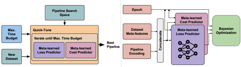
Figure 1: General input to Quick-Tune (left) and detailed input to the BO loop (right).

3.4 Meta-learning for Optimizing Pipelines

A crucial novelty of our paper is to transfer-learn BO surrogates from existing pipeline evaluations on other datasets. Assume we have access to a set of learning curves for the validation errors $\ell$ and the runtimes $c$ of pipelines over a pool of datasets, for a series of epochs. We call the collection of such quadruple evaluations a meta-dataset $H:=\bigcup_{x\in\mathcal{X}}\bigcup_{d\in\mathcal{D}}\bigcup_{e\in\mathbb{N}}\left\{\left(\left(x,e,\ell\left(x,d,e\right)\right),c\left(x,d,e\right)\right)\right\}$.

We meta-learn a probabilistic validation error estimator $\hat{\ell}\left(x,d,e;\theta\right)$, and a point-estimate cost predictor $\hat{c}\left(x,d,e;\gamma\right)$ from the meta-dataset $H$ by solving the following objective functions:

$$\theta^{\text{meta-learned}}\; :=\;\operatorname*{arg\,min}_{\theta}\;\mathbb{E}_{\left(x,e,\ell(x,d,e),c(x,d,e)\right)\sim H}\;\;\left[-\log p\left(\ell(x,d,e)\;|\;x,d,e,\hat{\ell}(x,d,e;\theta)\right)\right]$$ (5)

$$\gamma^{\text{meta-learned}}\; :=\;\operatorname*{arg\,min}_{\gamma}\;\mathbb{E}_{\left(p,x,\ell(x,d,e),c(x,d,e)\right)\sim H}\;\;\left(c(x,d,e)-\hat{c}\left(x,d,e;\gamma\right)\right)^{2}$$ (6)

After meta-learning the validation error and the runtime estimators, we transfer-learn them to conduct gray-box BO. The respective selection of the pipeline is transformed from Equation 4 into $\mathcal{A}^{\text{G-BO}}(H):=\operatorname*{arg\,max}_{x\in\mathcal{X}}\;\frac{a\left(x,d,e_{x}+1,\hat{\ell}\left(x,d,e_{x}+1;\;\theta^{\text{meta-learned}}\right)\right)}{\hat{c}\left(x,d,e_{x}+1;\;\gamma^{\text{meta-learned}}\right)}$. This enables us to transfer the knowledge about the performance of deep learning pipelines and their runtime costs in $H$ by means of utilizing the pretrained parameters $\theta^{\text{meta-learned}},\gamma^{\text{meta-learned}}$ when conducting BO on a new dataset.

The actual architecture of the estimators is presented in Figure 1. It is important to highlight that we do not input a full-dataset $d$ to the estimators. Instead, we use computed meta-features for $d$ that capture dataset characteristics. Additionally, our pipeline encoding is a concatenation of the hyperparameters $\lambda$, categorical embedding of the model name $m\in\mathcal{M}$ [19] and an embedding of the observed loss curve [62]. We provide more fine-grained details in Appendix A.

4 Quick-Tune Meta-Dataset

4.1 Quick-Tune Search Space

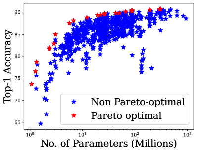
Figure 2: The subset of Pareto optimal pretrained models with respect to the predictive accuracy and model size.

While our proposed method is agnostic to the application domain, set of pretrained models and hyperparameter space to choose from, we need to instantiate these choices for our experiments. In this paper, we focus on the application domain of image classification and base our study on the timm library [58], given its popularity and wide adoption in the community. It contains a large set of hyperparameters and pretrained models on ImageNet (more than 700). Concerning the space of potential finetuning hyperparameters, we select a subset of optimizers and schedulers that are well-known and used by researchers and practitioners. We also include regularization techniques, such as data augmentation and drop-out, since finetuning is typically applied in low data regimes where large architectures easily overfit. Additionally, we modified the framework to include common finetuning strategies, such as methods that allow to select the percentage of layers to finetune [68], linear probing  [57], stochastic norm [29], Co-Tuning [69], DELTA [34], BSS [13] and SP-regularization [33]. The last five methods were taken from the transfer learning library [25]. Although we consider these well-known and stable finetuning strategies, we foresee the widespread adoption of new approaches such as LoRA [21]. They are complementary to our method and can be easily interpreted as an extension of the pipeline search space. Our search space of Table LABEL:tab:full_search_space includes hyperparameter ranges that are commonly used by researchers and practitioners. We list all the selected hyperparameters in Table 1, indicating explicitly the conditional hyperparameters with a "*". Further details on the considered values and hyperparameter dependencies are reported in Table LABEL:tab:full_search_space of Appendix D. As we are interested in time efficiency and accuracy, we select the Pareto optimal models from the large set of ca. $700$ pretrained architectures in the timm library. Specifically, given a model $m\in\mathcal{M}_{\mathrm{Timm}}$ with Top-1 ImageNet accuracy $f_{\mathrm{ImageNet}}(m)$ and $S(m)$ parameters, we build our final model hub based on the multi-objective optimization among the predictive accuracy and model size as:

$$\mathcal{M}=\left\{m^{*}\,|\,m^{*}\in\operatorname*{arg\,max}_{m\in\mathcal{M}_{\mathrm{Timm}}}\left[f_{\mathrm{ImageNet}}(m),\;-S(m)\right]\right\}$$ (7)

After solving the optimization problem in Equation 7, we obtain a set of 24 Pareto-optimal models as shown in Figure 2 and listed in Table 9 of Appendix D.

4.2 Meta-Dataset Generation

We created a large meta-dataset of evaluated learning curves based on the aforementioned search space. Overall, we finetuned the 24 Pareto-optimal pretrained models on 87 datasets for different hyperparameter configurations (details in Table LABEL:tab:metadataset_composition). For every dataset, we sample hyperparameter configurations and models uniformly at random from the search space of Table LABEL:tab:full_search_space. During sampling, we take into account the dependencies of the conditional hyperparameters. Every triple (model, dataset, hyperparameter configuration) resulted in a finetuning optimization run that produced a learning curve. Some of them were also infeasible to evaluate due to the model size, thus some triples might have fewer evaluations as detailed in Appendix B.

In our experiments, we use the tasks contained in the Meta-Album benchmark [56] because it contains a diverse set of computer vision datasets. The benchmark is released in three variants with an increasing number of images per dataset: micro, mini, and extended. Concretely, micro has computer vision tasks with fewer classes and fewer images per class than extended. When generating the learning curves, we limited each run to 50 training epochs. As setting a limit is challenging when considering a pool of models and tasks with different sizes, we decided to constrain the finetuning procedure using a global time limit. Specifically, the configurations trained on the tasks from micro, mini, extended are finetuned for 1, 4, and 16 hours respectively, using a single NVIDIA GeForce RTX 2080 Ti GPU per finetuning task, amounting to a total compute time of 32 GPU months. We summarize the main characteristics of our generated data in Table LABEL:tab:metadataset_composition.

Table 1: Search Space Summary.

Hyperparameter Group	Hyperparameters
Finetuning Strategies	Percentage of the Model to Freeze, Layer Decay, Linear Probing, Stochastic Norm, SP-Regularization, DELTA Regularization, BSS Regularization, Co-Tuning
Regularization Techniques	MixUp, MixUp Probability*, CutMix, Drop-Out, Label Smoothing, Gradient Clipping
Data Augmentation	Data Augmentation Type (Trivial Augment, Random Augment, Auto-Augment), Auto-Augment Policy*, Number of operations*, Magnitude*
Optimization	Optimizer type (SGD, SGD+Momentum, Adam, AdamW, Adamp), Beta-s*, Momentum*, Learning Rate, Warm-up Learning Rate, Weight Decay, Batch Size
Learning Rate Scheduling	Scheduler Type (Cosine, Step, Multi-Step, Plateau), Patience*, Decay Rate*, Decay Epochs*
Model	24 Models on the Pareto front (see Appendix 9)

Table 2: Quick-Tune Composition

Meta-Dataset	Number of Tasks	Number of Curves	Total Epochs	Total Run Time
Micro	30	8.712	371.538	2076 GPU Hours
Mini	30	6.731	266.384	6049 GPU Hours
Extended	27	4.665	105.722	15866 GPU Hours

5 Experiments and Results

5.1 Quick-Tune Protocol

While Quick-Tune finds the best-pretained models and their hyperparameters, it also has hyperparameters of its own: the architecture and the optimizer for the predictors, and the acquisition function. Before running the experiments, we aimed at designing a single setup that is readily applicable to all the tasks. Given that we meta-train the cost and loss predictor, we split the tasks per Meta-Album version into five folds $\mathcal{D}=\{\mathcal{D}_{1},...,\mathcal{D}_{5}\}$ containing an equal number of tasks. When searching for a pipeline on datasets of a given fold $\mathcal{D}_{i}$, we use one of the remaining folds for meta-validation and the remaining ones for meta-training. We used the meta-validation for early stopping when meta-training the predictors. We tune the hyperparameters of Quick-Tune’s architecture, as well as the learning rate, using the mini version’s meta-validation folds. For the sake of computational efficiency, we apply the same discovered hyperparameters in the experiments involving the other Meta-Album versions. The chosen setup uses an MLP with 2 hidden layers with 32 neurons for both predictors, and Adam Optimizer with learning rate of $10^{-4}$, both for meta-training, as well as surrogate fitting during the BO steps. Further details on the set-up are specified in Appendix A.2.

5.2 Research Hypothesis and Associated Experiments

Hypothesis 1: Quick-Tune is better than finetuning models using their default settings.

ML practitioners need to carefully tune hyperparameters if they want to obtain state-of-the-art performance. Due to computational and time limitations, a common choice is to use default hyperparameters. In order to simulate a practical use case, we select three different models from the subset of Pareto-optimal pretrained models (see Fig. 2), i.e. the top model (beit_large_patch16_512 [7]; 305M parameters, 90.69% acc.), the middle one (xcit_small_12_p8_384_dist [2]; 26M and 89.52%), as well as the smallest model (dla46x_c [72]; 1.3M and 72.61%). On each dataset in Meta-Album [56], we finetune these models with their default hyperparameters and compare their performance against Quick-Tune. The default configuration is specified in Appendix D.1. As a proxy to the loss, we measure the average normalized regret [4], computed as detailed in Appendix A.1. For all Meta-Album datasets in a given category, we use the same finetuning time budget, i.e. 1 (micro), 4 (mini), and 16 (extended) hours. As reported in Table LABEL:tab:experiment1, Quick-Tune outperforms the default setups in terms of both normalized regret and rank across all respective subset datasets, demonstrating that HPO tuning is not only important to obtain high performance, but also achievable on low time budget conditions.

Table 3: Performance comparison for Hypothesis 1. Normalized regret, ranks and standard deviations calculated across all respective Meta-Album [56] subset datasets.

	Normalized Regret			Rank
	Micro	Mini	Extended	Micro	Mini	Extended
BEiT+Default HP	$0.229_{\pm 0.081}$	$0.281_{\pm 0.108}$	$0.225_{\pm 0.059}$	$2.583_{\pm 0.829}$	$2.611_{\pm 0.465}$	$3.136_{\pm 0.215}$
XCiT+Default HP	$0.223_{\pm 0.075}$	$0.290_{\pm 0.107}$	$0.199_{\pm 0.057}$	$2.500_{\pm 0.751}$	$2.694_{\pm 0.264}$	$2.522_{\pm 0.344}$
DLA+Default HP	$0.261_{\pm 0.074}$	$0.325_{\pm 0.111}$	$0.219_{\pm 0.076}$	$3.062_{\pm 0.770}$	$3.138_{\pm 0.248}$	$2.977_{\pm 0.284}$
Quick-Tune	$\mathbf{0.153_{\pm 0.054}}$	$\mathbf{0.139_{\pm 0.112}}$	$\mathbf{0.052_{\pm 0.031}}$	$\mathbf{1.854_{\pm 1.281}}$	$\mathbf{1.555_{\pm 0.531}}$	$\mathbf{1.363_{\pm 0.376}}$

Hypothesis 2: Quick-Tune is more efficient than multi-fidelity HPO optimizers.

Multi-fidelity approaches are considered very practical, especially for optimizing expensive architectures. We compare Quick-Tune against three popular multi-fidelity optimizers, BOHB [16], ASHA [33], DEHB  [6] and DyHPO [62]. We additionally include Random Search [10] as a baseline for a sanity check. The normalized regret is computed for the three Meta-album versions on budgets of 1, 4 and 16 hours. The results of Figure 3 show that our proposed method has the best any-time performance compared to the baselines. In an additional experiment, presented in Figure 4, we show that both meta-training and cost-awareness aspects contribute to this goal by ablating each individual component. This behaviour is consistent among datasets of different sizes and present in all three meta-dataset versions. The search efficiency is attributed to our careful search space design, which includes both large and small models, as well as regularization techniques that reduce overfitting in low-data settings such as in the tasks of the micro version. In large datasets, our method finds good configurations even faster than the baselines, highlighting the importance of cost-awareness in optimizing hyperparameters for large datasets.

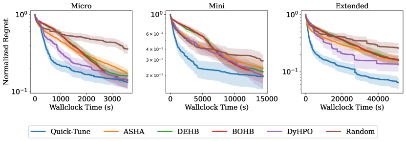
Figure 3: Results for Hypothesis 2.

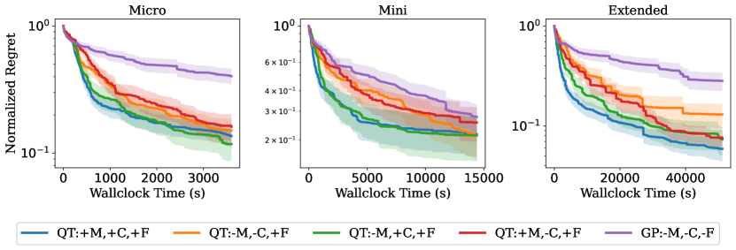
Figure 4: Ablation Studies: Comparing Quick-Tune with (+) and without (-) (M)eta-Surrogate and (C)ost-Awareness, and Multi-(F)idelity. We also compare against DyHPO(=QT:-M,-C,+F) and GP.

Hypothesis 3: CASH on diverse model hubs is better than HPO on a single model.

A reasonable question is whether we actually need to consider a hub of models at all, or whether perhaps using a single, expressive and well-tuned architecture is sufficient for most datasets. We hypothesize that the optimal model is dataset-specific because the complexities of datasets vary. Therefore, using a single model for all the datasets is a sub-optimal practice, and it is better to include a diverse model hub. Additionally, using a model hub allows to explore cheap models first, and gain information about the interactions between the hyperparameters that can be leveraged by the predictors when considering to observe the loss of a large but more accurate model.

To test this idea, we select EfficientNet [53] (with model name tf_efficientnet_b7_ns), X-Cit [2] and DLA [72]. These correspond to models with at least 10 evaluated curves in all the datasets and located on the top, middle and bottom regions in the Pareto front. Subsequently, we optimize their hyperparameters independently using our Quick-Tune algorithm. We also run Quick-Tune on subsets of 5, 10, and 15 models out of the model hub $\mathcal{M}$ with 24 models. The subset of models was created randomly for every dataset before running BO. We execute the optimization on the three meta-dataset versions for 1, 2 and 4 hours budget. Figure 5 demonstrates that, in general, it is better to have a pool of diverse models such as 24 models (24-M) or 15 models (15-M), than tuning a small set of models or even a unique model. Interestingly, we note the larger the dataset is, the larger the model hub we need. Considering only one model seems to offer an advantage on small datasets (micro), probably because it is possible to quickly observe more configurations than for larger datasets.

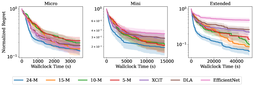
Figure 5: Results for Hypothesis 3.

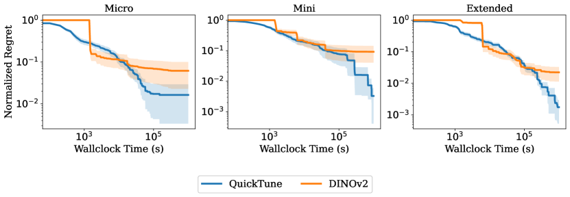
Figure 6: Results for Hypothesis 4.

Hypothesis 4: Quick-Tune outperforms finetuning state-of-the-art feature extractors.

A common practice is to use large feature extractors as the backbone and just train a linear output layer. We argue that selecting the model from a pool and optimizing its hyperparameters jointly is a more effective approach. Firstly, large backbones are often all-purpose models that may be inferior to model hubs when downstream tasks deviate largely from the backbone pretraining and may require non-trivial finetuning hyperparameter adaptations. As such, individual large models may violate the diversity property observed in our third hypothesis above. Secondly, due to their large number of parameters, they are expensive to optimize.

To show that selecting a model from a model hub with Quick-Tune is a more effective approach than using an all-purpose model, we compare to DINOv2’s [38] According to the method’s linear evaluation protocol, the procedure to classify downstream tasks with pretrained DINOv2 involves performing a small grid search over a subset of its finetuning hyperparameters (104 configurations in total including learning rate, number of feature extraction layers, etc.). We adopt this grid search in our comparison, evaluating the hyperparameter configurations on the grid in a random order. For each meta-album version, we then compare the normalized regret against the wall-clock time between DINOv2 and Quick-Tune. We increased Quick-Tune’s budget to match DINOv2’s budget requirements, since the evaluation of the full DINOv2 grid requires more time than our previous experiments. The results reported in Figure 6 show that Quick-Tune can significantly outperform finetuning state-of-the-art feature extractors such as DINOv2. Lastly, our method manages to find the best final configuration, which highlights the benefits of our designed search space. We refer to Appendix C for the full details on the comparison to DINOv2.

6 Conclusion

We tackle the practical problem of selecting a model and its hyperparameters given a pool of models. Our method QuickTune leverages multi-fidelity together with meta-learned cost and performance predictors in a Bayesian optimization setup. We demonstrate that QuickTune outperforms common strategies for selecting pretrained models, such as using single models, large feature extractors, or conventional HPO tuning methods. In addition, we presented empirical evidence that our method outperforms large-scale and state-of-the-art transformer backbones for computer vision. As a consequence, QuickTune offers a practical and efficient alternative for selecting and tuning pretrained models for image classification.

Appendix A Algorithmic Details

Input: Model hub $\mathcal{M}=\{m_{1},...,m_{|\mathcal{M}|}\}$, Search space of pipelines $x\in\mathcal{X}$, meta-dataset of pipeline losses and costs ${H}^{(M)}$, maximum time budget $T$, new dataset $d$, acquisition function $a$

Output: Finetuned pipeline $x^{*}$

1 Meta-train once the loss and cost predictors $\hat{\ell}$ and $\hat{c}$ on ${H}^{(M)}$ ;

2

3Initialize epoch counts $e_{x}=0$, observed losses and costs ${H}=\emptyset$, total time budget $t=0$ ;

4

5Select randomly a pipeline $x_{i}\in\mathcal{M}\times\Lambda=\mathcal{X}$ ;

6 while  $t\leq T$ do

7       Update epoch count $e_{x_{i}}\leftarrow e_{x_{i}}+1$;

8       Observe loss and cost $\ell_{i}\leftarrow\ell({x_{i},d,e_{x_{i}})}$, $c_{i}\leftarrow c({x_{i},d,e_{x_{i}}})$;

9       Update observations ${H}\leftarrow{H}\cup\{(x_{i},d,e_{x_{i}},\ell_{i},c_{i})\}$ ;

10       Fit $\hat{\ell}(x,d,e_{x})$ and $\hat{c}(x,d,e_{x})$ on ${H}$;

11       $x_{i}\leftarrow\operatorname*{arg\,max}_{x\in\mathcal{X}}\frac{a(x,d,e_{x}+1,\hat{\ell}(x,d,e_{x}+1))}{\hat{c}(x,d,e_{x}+1)}$;

12       Update total time costs including overhead $t_{oh}$: $t\leftarrow t+t_{\mathrm{oh}}+c_{i}$ ;

13      

14 end while

15

16Obtain best pipeline: $x^{*}=(m^{*},\lambda^{*})=x_{i}$, such that $i\in\operatorname*{arg\,min}_{i}\ell_{i}$ ;

17 return $x^{*}$;

Algorithm 1 Quick-Tune Algorithm

A.1 Normalized Regret

Given an observed performance $y$, the normalized regret is computed per datasets as follows:

$$y_{\mathrm{norm}}=\frac{y_{\mathrm{max}}-y}{y_{\mathrm{max}}-y_{\mathrm{min}}}$$ (8)

where $y_{\mathrm{max}},y_{\mathrm{min}}$ are respectively the maximum and minimum performances in the meta-dataset.

A.2 Quick-Tune Set-Up Details

The categorical encoder of the model is a linear layer with 4 output neurons, while the learning curve embedding is a convolutional neural network with two layers. For the rest of hyperparameters of the deep-kernel Gaussian process surrogate and the acquisition function, we followed the settings described in the respective publication [62] and always use this setup unless specified otherwise.

A.3 Meta-training Algorithms

We present the procedure for meta-training the cost and loss predictors in Algorithm 2. Basically, we sample random batches after choosing also randomly a dataset within our meta-dataset, then we update the parameters of each predictor so that it minimizes their respective losses. The same strategy is used when updating during BO, but with fewer iterations. We metaßtrain for 10000 iterations using Adam Optimizer with learning rate 0.0001.

Input: Metadata with precomputed losses and cost $H$ with datasets $D=\{d_{1},...,d_{N}\}$, learning rate $\mu$

Output: Meta-learned parameters $\theta,\gamma$

1 Random initialize parameters $\theta,\gamma$ for loss predictor $\ell(\cdot)$ and cost predictor $c(\cdot)$;

2 for $i\in\{1...E\}$ do

3       Sample dataset $d\sim p(D)$;

4       Define $H_{d}\subset H=\{s=(x_{i},d_{j},\ell_{i},c_{i})|s\in H,d_{i}=d\}$ ;

5       Get batch of $B$ pipelines with loss and costs on dataset $d$: $\{(x_{i},\ell_{i},c_{i})\}_{i=1,..,B}\sim H_{d}$ ;

6       Compute gradient $\delta\theta=-\nabla_{\theta}\mathrm{log}p(\ell|x,d,e,\hat{\ell})$ (Equation 5) ;

7       Compute gradient $\delta\gamma=\nabla_{\gamma}\left(c(x,d,e)-\hat{c}(x,d,e)\right)^{2}$ (Equation 6) ;

8       Update parameters $\theta=\theta-\mu\cdot\delta\theta$, $\gamma=\gamma-\mu\cdot\delta\gamma$

9 end for

return $\theta,\gamma$

Algorithm 2 Meta-training Algorithm

A.4 Meta-Features

Similar to previous work [39] we use descriptive meta-features of the dataset: number of samples, image resolution, number of channels, and number of classes. Any other technique for embedding datasets is compatible and orthogonal with our approach. We consider that researching about the best type of meta-features is an exciting research direction.

A.5 Pipeline Encoding

Inspired by previous work [3], our pipeline encoding is the concatenating of the hyperparameters $\lambda_{i}$, the categorical encoding of the model name $\mathcal{E}_{\mathrm{model}}(m_{i})$ and the embedding of the curves. Given the loss curve $\tilde{\ell}_{x_{i},e_{i}}=\{\ell(x_{i},d,j))\}_{j=1,...,e_{i}-1}$ or the cost curve $\tilde{c}_{x_{i},e_{i}}=\{c(x_{i},d,j)\}_{j=1,...,e_{i}-1}$, we obtain the respective encodings $\mathcal{E}_{\mathrm{loss}}(\tilde{\ell}_{x_{i},e_{i}})$ and $\mathcal{E}_{\mathrm{cost}}(\tilde{c}_{x_{i},e_{i}})$. The pipeline encoding is then defined as:

$$\mathrm{Pipeline\ Encondig}(x_{i})=[\lambda_{i},\mathcal{E}_{\mathrm{model}}(m_{i}),\mathcal{E}_{\mathrm{loss}}(\tilde{\ell}_{x_{i},e_{i}}),\mathcal{E}_{\mathrm{cost}}(\tilde{c}_{x_{i},e_{i}})]$$ (9)

The parameters of the encoders $\mathcal{E}_{\mathrm{model}}(\cdot),\mathcal{E}_{\mathrm{loss}}(\cdot),\mathcal{E}_{\mathrm{cost}}(\cdot)$ are jointly updated during meta-training and fitting the predictors while BO.

Appendix B Meta-Dataset Composition Details

Some pipelines failed due to the GPU requirements demanded by number of parameters of the model and the number of classes of the datasets. In that case, we decreased the batch size iteratively, halving the value, until it fit to the GPU. In some cases, this strategy was not enough, thus some models have more evaluations than others. In Table 4, we present the list of datasets per set, and indicated (*) the heavy datasets, i.e. with a lot of classes or a lot of samples in the extended version. All datasets are present in three versions, except the underlined ones, which are not present in the extended version. The OpenML Ids associated to the datasets are listed in Table 5.

Table 4: Datasets per Set in Meta-Album

Set	Dataset Names
0	BCT, BRD*, CRS, FLW, MD_MIX, PLK*, PLT_VIL*, RESISC, SPT, TEX
1	ACT_40, APL, DOG, INS_2*, MD_5_BIS, MED_LF, PLT_NET*, PNU, RSICB, TEX_DTD
2	ACT_410, AWA*, BTS*, FNG, INS*, MD_6, PLT_DOC, PRT, RSD*, TEX_ALOT*

Table 5: OpenML IDs for Datasets per Split and Version

Version	Set 0	Set 1	Set 2
Micro	44241, 44238, 44239, 44242, 44237, 44246, 44245, 44244, 44240, 44243	44313, 44248, 44249, 44314, 44312, 44315, 44251, 44250, 44247, 44252	44275, 44276, 44272, 44273, 44278, 44277, 44279, 44274, 44271, 44280
Mini	44285, 44282, 44283, 44286, 44281, 44290, 44289, 44288, 44284, 44287	44298, 44292, 44293, 44299, 44297, 44300, 44295, 44294, 44291, 44296	44305, 44306, 44302, 44303, 44308, 44307, 44309, 44304, 44301, 44310
Extended	44320, 44317, 44318, 44321, 44316, 44324, 44323, 44322, 44319	44331, 44326, 44327, 44332, 44330, 44333, 44329, 44328, 44325	44338, 44340, 44335, 44336, 44342, 44341, 44343, 44337, 44334

Appendix C DINOv2 Details

When running DINOv2, we select a configuration from the DINOv2 grid at random for each Meta-Album subset dataset, we run that configuration until the end. Subsequently we iterate by selecting the next configurations at random until we exhausted all the configurations in the grid proposed by the authors. In the following, we depict which of the datasets we ran with the default hyperparameter configuration according to [38] and which we adapted due to the single-GPU constraint (RTX2080). Runs indicated with "*" failed due to GPU memory limitations and for runs indicated by "n_last_blocks=1" we ran with the default hyperparameters except for the "n_last_blocks" argument that had to be changed from 4 to 1 to fit on the GPU.

Table 6: Subset Micro

Dataset	Linear Eval. Hyp.
micro_set0_BCT	DINOv2 default
micro_set0_BRD	DINOv2 default
micro_set0_CRS	DINOv2 default
micro_set0_FLW	DINOv2 default
micro_set0_MD_MIX	DINOv2 default
micro_set0_PLK	DINOv2 default
micro_set0_PLT_VIL	DINOv2 default
micro_set0_RESISC	DINOv2 default
micro_set0_SPT	DINOv2 default
micro_set0_TEX	DINOv2 default
micro_set1_ACT_40	DINOv2 default
micro_set1_APL	DINOv2 default
micro_set1_DOG	DINOv2 default
micro_set1_INS_2	DINOv2 default
micro_set1_MD_5_BIS	DINOv2 default
micro_set1_MED_LF	DINOv2 default
micro_set1_PLT_NET	DINOv2 default
micro_set1_PNU	DINOv2 default
micro_set1_RSICB	DINOv2 default
micro_set1_TEX_DTD	DINOv2 default
micro_set2_ACT_410	DINOv2 default
micro_set2_AWA	DINOv2 default
micro_set2_BTS	DINOv2 default
micro_set2_FNG	DINOv2 default
micro_set2_INS	DINOv2 default
micro_set2_MD_6	DINOv2 default
micro_set2_PLT_DOC	DINOv2 default
micro_set2_PRT	DINOv2 default
micro_set2_RSD	DINOv2 default
micro_set2_TEX_ALOT	DINOv2 default

Table 7: Subset Mini

Dataset	Linear Eval. Hyp.
mini_set0_BCT	DINOv2 default
mini_set0_BRD	n_last_blocks=1
mini_set0_CRS	n_last_blocks=1
mini_set0_FLW	DINOv2 default
mini_set0_MD_MIX	n_last_blocks=1
mini_set0_PLK	DINOv2 default
mini_set0_PLT_VIL	DINOv2 default
mini_set0_RESISC	DINOv2 default
mini_set0_SPT	DINOv2 default
mini_set0_TEX	DINOv2 default
mini_set1_ACT_40	DINOv2 default
mini_set1_APL	DINOv2 default
mini_set1_DOG	n_last_blocks=1
mini_set1_INS_2	n_last_blocks=1
mini_set1_MD_5_BIS	n_last_blocks=1
mini_set1_MED_LF	DINOv2 default
mini_set1_PLT_NET	DINOv2 default
mini_set1_PNU	DINOv2 default
mini_set1_RSICB	DINOv2 default
mini_set1_TEX_DTD	DINOv2 default
mini_set2_ACT_410	DINOv2 default
mini_set2_AWA	DINOv2 default
mini_set2_BTS	DINOv2 default
mini_set2_FNG	DINOv2 default
mini_set2_INS	n_last_blocks=1
mini_set2_MD_6	n_last_blocks=1
mini_set2_PLT_DOC	DINOv2 default
mini_set2_PRT	DINOv2 default
mini_set2_RSD	DINOv2 default
mini_set2_TEX_ALOT	n_last_blocks=1

Table 8: Subset Extended

Dataset	Linear Eval. Hyp.
extended_set0_BCT	n_last_blocks=1
extended_set0_CRS	n_last_blocks=1
extended_set0_FLW	n_last_blocks=1
extended_set0_RESISC	n_last_blocks=1
extended_set0_SPT	n_last_blocks=1
extended_set0_TEX	n_last_blocks=1
extended_set1_ACT_40	DINOv2 default
extended_set1_APL	n_last_blocks=1
extended_set1_DOG	n_last_blocks=1
extended_set2_ACT_410	DINOv2 default
extended_set2_PLT_DOC	DINOv2 default
extended_set0_BRD	*
extended_set0_PLK	*
extended_set0_PLT_VIL	*
extended_set1_INS_2	*
extended_set1_MED_LF	n_last_blocks=1
extended_set1_PLT_NET	*
extended_set1_PNU	n_last_blocks=1
extended_set1_RSICB	*
extended_set1_TEX_DTD	n_last_blocks=1
extended_set2_AWA	*
extended_set2_BTS	*
extended_set2_FNG	n_last_blocks=1
extended_set2_PRT	n_last_blocks=1
extended_set2_RSD	*
extended_set2_TEX_ALOT	n_last_blocks=1
extended_set2_INS	*

Appendix D Search Space Details

D.1 Default Configuration

We report the hyperparameters for the default configuration in Experiment 1 by using bold font in Table LABEL:tab:full_search_space.

D.2 Model Hub

We list all the models on the Pareto Front from Timm’s library as provided on version 0.7.0dev0. Moreover, we report their size (number of parameters) and the top-1 accuracy in ImageNet.

Table 9: Models on the pareto front

Model Name	No. of Param.	Top-1 Acc.
beit_large_patch16_512	305.67	90.691
volo_d5_512	296.09	90.610
volo_d5_448	295.91	90.584
volo_d4_448	193.41	90.507
swinv2_base_window12to24_192to384_22kft1k	87.92	90.401
beit_base_patch16_384	86.74	90.371
volo_d3_448	86.63	90.168
tf_efficientnet_b7_ns	66.35	90.093
convnext_small_384_in22ft1k	50.22	89.803
tf_efficientnet_b6_ns	43.04	89.784
volo_d1_384	26.78	89.698
xcit_small_12_p8_384_dist	26.21	89.515
deit3_small_patch16_384_in21ft1k	22.21	89.367
tf_efficientnet_b4_ns	19.34	89.303
xcit_tiny_24_p8_384_dist	12.11	88.778
xcit_tiny_12_p8_384_dist	6.71	88.101
edgenext_small	5.59	87.504
xcit_nano_12_p8_384_dist	3.05	85.025
mobilevitv2_075	2.87	82.806
edgenext_x_small	2.34	81.897
mobilevit_xs	2.32	81.574
edgenext_xx_small	1.33	78.698
mobilevit_xxs	1.27	76.602
dla46x_c	1.07	73.632

D.3 Hyperparameter Search Space

Table LABEL:tab:full_search_space shows the complete search space of hyperparameters. During the curve generation, we sample uniformly among these discrete values. Some hyperparameters are conditional, i.e. their are only present when another hyperparameter gets a specific set of values. Thus, we also list explicitly which are the conditions for such hyperparameters.

Table 10: Detailed Search Space for Curve Generation. Bold font indicates the default configuration.

Hyperparameter Group	Name	Options	Conditional
Fine-Tuning Strategies	Percentage to freeze	0, 0.2, 0.4, 0.6, 0.8, 1
	Layer Decay	None, 0.65, 0.75	-
	Linear Probing	True, False	-
	Stochastic Norm	True, False	-
	SP-Regularization	0, 0.0001, 0.001, 0.01, 0.1	-
	DELTA Regularization	0, 0.0001, 0.001, 0.01, 0.1	-
	BSS Regularization	0, 0.0001, 0.001, 0.01, 0.1	-
	Co-Tuning	0, 0.5, 1, 2, 4	-
Regularization Techniques	MixUp	0, 0.2, 0.4, 1, 2, 4, 8
	MixUp Probability	0, 0.25, 0.5, 0.75, 1	-
	CutMix	0, 0.1, 0.25, 0.5, 1,2,4	-
	DropOut	0, 0.1, 0.2, 0.3, 0.4	-
	Label Smoothing	0, 0.05, 0.1	-
	Gradient Clipping	None, 1, 10	-
Data Augmentation	Data Augmentation	None, trivial_augment, random_augment, auto_augment	-
	Auto Augment	None, v0, original	-
	Number of Operations	2,3	Data Augmentation (Random Augment)
	Magnitude	9, 17	Data Augmentation (Random Augment)
Optimizer Related	Optimizer Type	SGD, SGD+Momentum, Adam, AdamW, Adamp	-
	Betas	(0.9, 0.999), (0, 0.99), (0.9, 0.99), (0, 0.999)	Scheduler Type (Adam, Adamw, Adamp)
	Learning Rate	0.1,0.01, 0.005, 0.001, 0.0005, 0.0001, 0.00005, 0.00001	-
	Warm-Up Learning Rate	0, 0.000001, 0.00001	-
	Weight Decay	0, 0.00001, 0.0001, 0.001, 0.01,0.1	-
	Batch Size	2,4,8,16,32,64,128,256,512	-
	Momeutm	0, 0.8, 0.9, 0.95, 0.99	Optimizer Type (SGD+Momentum)
Scheduler Related	Scheduler Type	None, Cosine, Step, Multistep, Plateau	-
	Patience	2,5	Scheduler Type (Plateau)
	Decay Rate	0.1, 0.5	Scheduler Type (Step, Multistep)
	Decay Epochs	10, 20	Scheduler Type (Step, Multistep)
Model	Model	See Table 9

References

- [1] S. Abnar, M. Dehghani, B. Neyshabur, and H. Sedghi. Exploring the limits of large scale pre-training. In Proc. of ICLR’22, 2022.
- [2] Alaaeldin Ali, Hugo Touvron, Mathilde Caron, Piotr Bojanowski, Matthijs Douze, Armand Joulin, Ivan Laptev, Natalia Neverova, Gabriel Synnaeve, Jakob Verbeek, et al. Xcit: Cross-covariance image transformers. Advances in neural information processing systems, 34:20014–20027, 2021.
- [3] Sebastian Pineda Arango and Josif Grabocka. Deep pipeline embeddings for automl. arXiv preprint arXiv:2305.14009, 2023.
- [4] Sebastian Pineda Arango, Hadi S. Jomaa, Martin Wistuba, and Josif Grabocka. Hpo-b: A large-scale reproducible benchmark for black-box hpo based on openml, 2021.
- [5] N. Awad, N. Mallik, and F. Hutter. DEHB: Evolutionary hyberband for scalable, robust and efficient Hyperparameter Optimization. In Proc. of IJCAI’21, pages 2147–2153, 2021.
- [6] Noor H. Awad, Neeratyoy Mallik, and Frank Hutter. DEHB: evolutionary hyberband for scalable, robust and efficient hyperparameter optimization. CoRR, abs/2105.09821, 2021.
- [7] Hangbo Bao, Li Dong, Songhao Piao, and Furu Wei. Beit: BERT pre-training of image transformers. In The Tenth International Conference on Learning Representations, ICLR 2022, Virtual Event, April 25-29, 2022. OpenReview.net, 2022.
- [8] Y. Bao, Y. Li, S.-L. Huang, L. Zhang, L. Zheng, A. Zamir, and L. J. Guibas. An information-theoretic approach to transferability in task transfer learning. In 2019 IEEE International Conference on Image Processing, ICIP 2019, Taipei, Taiwan, September 22-25, 2019, pages 2309–2313. IEEE, 2019.
- [9] J. Bergstra and Y. Bengio. Random search for hyper-parameter optimization. 13:281–305, 2012.
- [10] James Bergstra and Yoshua Bengio. Random search for hyper-parameter optimization. J. Mach. Learn. Res., 13:281–305, 2012.
- [11] D. Bolya, R. Mittapalli, and J. Hoffman. Scalable diverse model selection for accessible transfer learning. In Proc. of NeurIPS’21, pages 19301–19312, 2021.
- [12] Wei-Yu Chen, Yen-Cheng Liu, Zsolt Kira, Yu-Chiang Frank Wang, and Jia-Bin Huang. A closer look at few-shot classification. arXiv preprint arXiv:1904.04232, 2019.
- [13] X. Chen, S. Wang, B. F., M. Long, and J. Wang. Catastrophic forgetting meets negative transfer: Batch spectral shrinkage for safe transfer learning. In Proc. of NeurIPS’19, pages 1906–1916, 2019.
- [14] Y. Cui, Y. Song, C. Sun, A. Howard, and S. J. Belongie. Large scale fine-grained categorization and domain-specific transfer learning. In Proc. of CVPR’18, pages 4109–4118, 2018.
- [15] S. Falkner, A. Klein, and F. Hutter. BOHB: Robust and efficient Hyperparameter Optimization at scale. In Proc. of ICML’18, pages 1437–1446, 2018.
- [16] Stefan Falkner, Aaron Klein, and Frank Hutter. BOHB: robust and efficient hyperparameter optimization at scale. In Proceedings of the 35th International Conference on Machine Learning, ICML 2018, Stockholmsmässan, Stockholm, Sweden, July 10-15, 2018, pages 1436–1445, 2018.
- [17] M. Feurer, J. Springenberg, and F. Hutter. Initializing Bayesian Hyperparameter Optimization via meta-learning. In Proc. of AAAI’15, pages 1128–1135, 2015.
- [18] R. Garnett. Bayesian Optimization. Cambridge University Press, 2022. in preparation.
- [19] C. Guo and F. Berkhahn. Entity embeddings of categorical variables. arXiv:1604.06737 [cs.LG], 2016.
- [20] Y. Guo, H. Shi, A. Kumar, K. Grauman, T. Rosing, and R. S. Feris. Spottune: Transfer learning through adaptive fine-tuning. In Proc. of CVPR’19, pages 4805–4814, 2019.
- [21] Edward J. Hu, Yelong Shen, Phillip Wallis, Zeyuan Allen-Zhu, Yuanzhi Li, Shean Wang, and Weizhu Chen. Lora: Low-rank adaptation of large language models. CoRR, abs/2106.09685, 2021.
- [22] F. Hutter, H. Hoos, and K. Leyton-Brown. Sequential model-based optimization for general algorithm configuration. In Proc. of LION’11, pages 507–523, 2011.
- [23] F. Hutter, L. Kotthoff, and J. Vanschoren, editors. Automated Machine Learning: Methods, Systems, Challenges. Springer, 2019. Available for free at http://automl.org/book.
- [24] H. Jomaa, L. Schmidth-Thieme, and J. Grabocka. Dataset2vec: Learning dataset meta-features. Data Mining and Knowledge Discovery, 35:964–985, 2021.
- [25] Bo Fu Junguang Jiang, Baixu Chen and Mingsheng Long. Transfer-learning-library. https://github.com/thuml/Transfer-Learning-Library, 2020.
- [26] A. S. Khazi, S. Pineda Arango, and J. Grabocka. Deep ranking ensembles for hyperparameter optimization. In The Eleventh International Conference on Learning Representations, 2023.
- [27] A. Kirillov, E. Mintun, N. Ravi, H. Mao, C. Rolland, L. Gustafson, T. Xiao, S. Whitehead, A. C. Berg, W. Lo, P. Dollár, and R. Girshick. Segment anything. arXiv:2304.02643, 2023.
- [28] A. Kolesnikov, L. Beyer, X. Zhai, J. Puigcerver, J. Yung, S. Gelly, and N. Houlsby. Big transfer (bit): General visual representation learning. In Proc. of ECCV’20, pages 491–507, 2020.
- [29] Z. Kou, K. You, M. Long, and J. Wang. Stochastic normalization. In Proc. of NeurIPS’20, 2020.
- [30] Y. Lee, A. S. Chen, F. Tajwar, A. Kumar, H. Yao, P. Liang, and C. Finn. Surgical fine-tuning improves adaptation to distribution shifts. CoRR, abs/2210.11466, 2022.
- [31] H. Li, P. Chaudhari, H. Yang, M. Lam, A. Ravichandran, R. Bhotika, and S. Soatto. Rethinking the hyperparameters for fine-tuning. In Proc. of ICLR’20, 2020.
- [32] L. Li, K. Jamieson, G. DeSalvo, A. Rostamizadeh, and A. Talwalkar. Hyperband: Bandit-based configuration evaluation for Hyperparameter Optimization. In Proc. of ICLR’17, 2017.
- [33] X. Li, Y. Grandvalet, and F. Davoine. Explicit inductive bias for transfer learning with convolutional networks. In Proc. of ICML’18, pages 2830–2839, 2018.
- [34] Xingjian Li, Haoyi Xiong, Hanchao Wang, Yuxuan Rao, Liping Liu, and Jun Huan. Delta: Deep learning transfer using feature map with attention for convolutional networks. In 7th International Conference on Learning Representations, ICLR 2019, New Orleans, LA, USA, May 6-9, 2019. OpenReview.net, 2019.
- [35] B. Liu, Y. Cai, Y. Guo, and X. Chen. Transtailor: Pruning the pre-trained model for improved transfer learning. In Proc. of AAAI’21, pages 8627–8634, 2021.
- [36] T. Mahmud, N. Frumkin, and D. Marculescu. Rl-tune: A deep reinforcement learning assisted layer-wise fine-tuning approach for transfer learning. In First Workshop on Pre-training: Perspectives, Pitfalls, and Paths Forward at ICML 2022, 2022.
- [37] C. V. Nguyen, T. Hassner, M. W. Seeger, and Cédric Archambeau. LEEP: A new measure to evaluate transferability of learned representations. In Proc. of ICML’20, volume 119, pages 7294–7305, 2020.
- [38] M. Oquab, T. Darcet, T. Moutakanni, H. V. Vo, M. Szafraniec, V. Khalidov, P. Fernandez, D. Haziza, F. Massa, A. El-Nouby, R. Howes, P.-Y. Huang, H. Xu, V. Sharma, S.-W. Li, W. Galuba, M. Rabbat, M. Assran, N. Ballas, G. Synnaeve, I. Misra, H. Jegou, J. Mairal, P. Labatut, A. Joulin, and P. Bojanowski. Dinov2: Learning robust visual features without supervision, 2023.
- [39] E. Öztürk, F. Ferreira, H. S. Jomaa, L. Scmidth-Thieme, J. Grabocka, and F. Hutter. Zero-shot automl with pretrained models. In Proc. of ICML’22, pages 1128–1135, 2022.
- [40] A. Radford, J. Wook Kim, C. Hallacy, Aditya Ramesh, G. Goh, S. Agarwal, G. Sastry, A. Askell, P. Mishkin, J. Clark, G. Krueger, and I. Sutskever. Learning transferable visual models from natural language supervision, 2021.
- [41] R. Ramesh and P. Chaudhari. Model zoo: A growing brain that learns continually. In Proc. of ICLR’22, 2022.
- [42] C. Rasmussen and C. Williams. Gaussian Processes for Machine Learning. The MIT Press, 2006.
- [43] D. Salinas, H. Shen, and V. Perrone. A quantile-based approach for hyperparameter transfer learning. In Proc. of ICML’20, pages 8438–8448, 2020.
- [44] K. Schürholt, B. Knyazev, X. Giró-i-Nieto, and D. Borth. Hyper-representations for pre-training and transfer learning. CoRR, abs/2207.10951, 2022.
- [45] K. Schürholt, D. Taskiran, B. Knyazev, X. Giró-i Nieto, and D. Borth. Model zoos: A dataset of diverse populations of neural network models. In Thirty-Sixth Conference on Neural Information Processing Systems (NeurIPS) Track on Datasets and Benchmarks, 2022.
- [46] G. Shala, A. Biedenkapp, F. Hutter, and J. Grabocka. Gray-box gaussian processes for automated reinforcement learning. In ICLR 2023.
- [47] G. Shala, T. Elsken, F. Hutter, and J. Grabocka. Transfer NAS with meta-learned bayesian surrogates. In ICLR 2023.
- [48] Z. Shen, Z. Liu, J. Qin, M. Savvides, and K.-T. Cheng. Partial is better than all: Revisiting fine-tuning strategy for few-shot learning. In Proc. of AAAI’21, pages 9594–9602, 2021.
- [49] Y. Shu, Z. Cao, Z. Zhang, J. Wang, and M. Long. Hub-pathway: Transfer learning from A hub of pre-trained models. 2022.
- [50] Y. Shu, Z. Kou, Z. Cao, J. Wang, and M. Long. Zoo-tuning: Adaptive transfer from A zoo of models. In Proc. of ICML’21, volume 139, pages 9626–9637, 2021.
- [51] J. Snoek, O. Rippel, K. Swersky, R. Kiros, N. Satish, N. Sundaram, M. Patwary, Prabhat, and R. Adams. Scalable Bayesian optimization using deep neural networks. In Proc. of ICML’15, pages 2171–2180, 2015.
- [52] J. Springenberg, A. Klein, S. Falkner, and F. Hutter. Bayesian optimization with robust Bayesian neural networks. In D. Lee, M. Sugiyama, U. von Luxburg, I. Guyon, and R. Garnett, editors, Proc. of NeurIPS’16, 2016.
- [53] Mingxing Tan and Quoc V. Le. Efficientnet: Rethinking model scaling for convolutional neural networks. In Kamalika Chaudhuri and Ruslan Salakhutdinov, editors, Proceedings of the 36th International Conference on Machine Learning, ICML 2019, 9-15 June 2019, Long Beach, California, USA, volume 97 of Proceedings of Machine Learning Research, pages 6105–6114. PMLR, 2019.
- [54] C. Thornton, F. Hutter, H. Hoos, and K. Leyton-Brown. Auto-WEKA: combined selection and Hyperparameter Optimization of classification algorithms. In Proc. of KDD’13, pages 847–855, 2013.
- [55] A. T. Tran, C. V. Nguyen, and T. Hassner. Transferability and hardness of supervised classification tasks. In Proc. of ICCV’19, pages 1395–1405. IEEE, 2019.
- [56] Ihsan Ullah, Dustin Carrion, Sergio Escalera, Isabelle M Guyon, Mike Huisman, Felix Mohr, Jan N van Rijn, Haozhe Sun, Joaquin Vanschoren, and Phan Anh Vu. Meta-album: Multi-domain meta-dataset for few-shot image classification. In Thirty-sixth Conference on Neural Information Processing Systems Datasets and Benchmarks Track, 2022.
- [57] H. Wang, T. Yue, X. Ye, Z. He, B. Li, and Y. Li. Revisit finetuning strategy for few-shot learning to transfer the emdeddings. In The Eleventh International Conference on Learning Representations, 2023.
- [58] Ross Wightman. Pytorch image models. https://github.com/rwightman/pytorch-image-models, 2019.
- [59] J. Wilson, F. Hutter, and M. Deisenroth. Maximizing acquisition functions for Bayesian optimization. In Proc. of NeurIPS’18, pages 741–749, 2018.
- [60] F. Winkelmolen, N. Ivkin, H. Bozkurt, and Z. Karnin. Practical and sample efficient zero-shot HPO. arXiv:2007.13382 [stat.ML], 2020.
- [61] M. Wistuba and J. Grabocka. Few-shot bayesian optimization with deep kernel surrogates. In Proc. of ICLR’21, 2021.
- [62] M. Wistuba, A. Kadra, and J. Grabocka. Supervising the multi-fidelity race of hyperparameter configurations. In Proc. of NeurIPS’22, 2022.
- [63] M. Wistuba, N. Schilling, and L. Schmidt-Thieme. Sequential Model-free Hyperparameter Tuning. In Proc. of ICDM ’15, pages 1033–1038, 2015.
- [64] M. Wistuba, N. Schilling, and L. Schmidt-Thieme. Two-stage transfer surrogate model for automatic Hyperparameter Optimization. In Proc. of ECML/PKDD’16, pages 199–214, 2016.
- [65] Martin Wistuba and Josif Grabocka. Few-shot bayesian optimization with deep kernel surrogates. In 9th International Conference on Learning Representations, ICLR 2021, Virtual Event, Austria, May 3-7, 2021, 2021.
- [66] M. Wortsman, G. Ilharco, S.r Yitzhak Gadre, R. Roelofs, R. Gontijo Lopes, A. S. Morcos, H. Namkoong, A. Farhadi, Y. Carmon, S. Kornblith, and L. Schmidt. Model soups: averaging weights of multiple fine-tuned models improves accuracy without increasing inference time. In Proc. of ICML’22, volume 162, pages 23965–23998, 2022.
- [67] M. Wortsman, G. Ilharco, J. W. Kim, M. Li, S. Kornblith, R. Roelofs, R. G. Lopes, H. Hajishirzi, A. Farhadi, H. Namkoong, and L. Schmidt. Robust fine-tuning of zero-shot models. In Proc. of CVPR’22, pages 7949–7961, 2022.
- [68] J. Yosinski, J. Clune, Y. Bengio, and H. Lipson. How transferable are features in deep neural networks? In Proc. of NeurIPS’14, pages 3320–3328, 2014.
- [69] K. You, Z. Kou, M. Long, and J. Wang. Co-tuning for transfer learning. In Proc. of NeurIPS’20, pages 17236–17246, 2020.
- [70] K. You, Y. Liu, J. Wang, M. I. Jordan, and M. Long. Ranking and tuning pre-trained models: A new paradigm of exploiting model hubs. CoRR, abs/2110.10545, 2021.
- [71] K. You, Y. Liu, J. Wang, and M. Long. Logme: Practical assessment of pre-trained models for transfer learning. In Proc. of ICML’21, pages 12133–12143, 2021.
- [72] Fisher Yu, Dequan Wang, Evan Shelhamer, and Trevor Darrell. Deep layer aggregation. In Proceedings of the IEEE conference on computer vision and pattern recognition, pages 2403–2412, 2018.
- [73] J. Zhong, X. Wang, Z. Kou, J. Wang, and M. Long. Bi-tuning of pre-trained representations. arXiv preprint arXiv:2011.06182, 2020.