Pre-training Tensor-Train Networks Facilitates Machine Learning with Variational Quantum Circuits

Abstract

Variational quantum circuit (VQC) is a promising approach for implementing quantum neural networks on noisy intermediate-scale quantum (NISQ) devices. Recent studies have shown that a tensor-train network (TTN) for VQC, namely TTN-VQC, can improve the representation and generalization powers of VQC. However, the Barren Plateau problem leads to the gradients of the cost function vanishing exponentially small as the number of qubits increases, making it difficult to find the optimal parameters for the VQC. To address this issue, we put forth a new learning approach called Pre+TTN-VQC that builds upon the TTN-VQC architecture by incorporating a pre-trained TTN to alleviate the Barren Plateau problem. The pre-trained TTN allows for efficient fine-tuning of target data, which reduces the depth of the VQC required to achieve good empirical performance and potentially alleviates the training obstacles posed by the Barren Plateau landscape. Furthermore, we highlight the advantages of Pre+TTN-VQC in terms of representation and generalization powers by exploiting the error performance analysis. Moreover, we characterize the optimization performance of Pre+TTN-VQC without the need for the Polyak-Lojasiewicz condition, thereby enhancing the practicality of implementing quantum neural networks on NISQ devices. We conduct experiments on a handwritten digit classification dataset to corroborate our proposed methods and theorems.

1 Introduction

Quantum machine learning (QML) is an emerging interdisciplinary field that integrates the principles of quantum mechanics and machine learning. With the rapid advances in quantum computing, we have witnessed the noisy intermediate-scale quantum (NISQ) era that admits as many as a few hundred qubits available for implementing many QML algorithms on real quantum computers to enhance the efficiency and speed of machine learning applications [33, 17, 39]. Despite the limitations of the NISQ era, which is characterized by a small number of qubits and high levels of quantum noise, we are exploring the potential of quantum computing for machine learning [4, 8, 7, 38, 16, 47, 26]. One of the most promising areas of QML is a quantum neural network (QNN) [1, 11, 22], a classical neural network quantum analog. QNN uses variational quantum circuits (VQC) as the building blocks for processing data and making predictions [9, 29, 10, 3, 40, 25]. VQC denotes a parameterized quantum circuit that can be optimized using classical optimization algorithms like stochastic gradient descent (SGD) to minimize the cost function in a back-propagation manner. The SGD algorithm has demonstrated that the VQC can be resilient to the quantum noise on NISQ devices [2, 14, 41], highlighting the advantages of deploying VQC for implementing QNN in many machine learning tasks [48, 21, 42, 34, 31, 27].

However, the Barren Plateau problem is a significant challenge in the training of VQC using the SGD algorithm [28, 15]. In particular, when the number of depths or qubits in a VQC is large, the gradients of the cost function can vanish exponentially, making it challenging to optimize the VQC parameters. From an optimization perspective, there have been various quantum-aware optimization approaches being explored to address the Barren Plateau problem, such as the introduction of carefully designed random initializations [50], the use of non-adaptive gradient methods [49], and the implementation of more sophisticated optimization techniques like the adaptive moment estimation algorithm [24]. Moreover, the use of quantum natural gradient descent  [43], which is based on the geometry of the quantum state space, can help mitigate the Barren Plateau problem in the training process of VQC.

Our previous work proposed a tensor-train network (TTN) [32] to construct a TTN-VQC model that alleviates the Barren Plateau landscape and makes the VQC training more feasible on NISQ devices [37]. Compared with the quantum-aware optimization methods, the TTN can inherently conduct dimensionality reduction and also introduces non-linearity to the input features such that the representation power of VQC can be greatly enhanced. Moreover, the TTN relies on a Polyak-Lojasiewicz (PL) assumption [23] that alleviates the Barren Plateau problem, thereby reducing the optimization bias to a small scale in the training process.

Besides, we highlight the theoretical advantages of TTN-VQC in terms of representation and generalization powers. The representation power refers to the ability of a model to approximate a target function for pattern classification, and the generalization power denotes the model’s capability to adapt properly to new, previously unseen data, drawn from the same distribution as the one used to create the model. Both the representation and generalization powers can be employed to compare the theoretical performance of QML models. Our previous work [37] justifies that TTN-VQC can achieve better representation and generalization powers than a VQC model based on the obtained theoretical and empirical results.

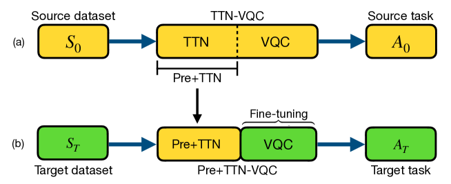
Figure 1: A demonstration of learning pipeline for Pre+TTN-VQC. (a) An illustration of a generic TTN-VQC trained on the source dataset $S_{0}$ for the source task $A_{0}$; (b) the pre-trained TTN is transferred to build up a Pre+TTN-VQC architecture, where the Pre+TTN is frozen and the VQC model need a further fine-tuned on the target dataset $S_{T}$ for the target task $A_{T}$. Besides, the data in $S_{0}$ does not overlap with $S_{T}$, but the classified patterns of $S_{T}$ are subsets of $S_{0}$.

Despite the advantages of TTN-VQC, the PL assumption for TTN-VQC is a sufficient but not necessary condition to alleviate the Barren Plateau problem. Given a constant factor $\mu$ and an empirical loss function $\mathcal{L}_{S}$ with respect to a model parameter $\boldsymbol{\theta}$, the PL condition for $\mathcal{L}_{S}(\boldsymbol{\theta})$ requires the following inequality as:

$$\frac{1}{2}\lVert\nabla\mathcal{L}_{S}(\boldsymbol{\theta})\rVert_{2}^{2}\geq\mu\mathcal{L}_{S}(\boldsymbol{\theta}).$$ (1)

However, the PL condition associated with Eq. (1) is not always satisfied on machine learning datasets, and exploring other approaches to overcome the Barren Plateau landscape is essential.

Thus, this work introduces a pre-training methodology for TTN on top of the TTN-VQC architecture named Pre+TTN-VQC. The pre-training approach has been widely applied to state-of-the-art deep learning technologies, especially in the fields of large language models [46, 5, 19]. Figure 1 illustrates a Pre+TTN-VQC architecture that is composed of a pre-trained TTN for feature abstraction of input data and a VQC classifier for making predictions. The pre-trained TTN is from a well-trained generic TTN-VQC on the source dataset $S_{0}$, and the VQC parameters are adjusted by using the technique of fine-tuning on the target dataset $S_{T}$. To avoid the issue of data distribution shift [45, 18], we assume that the dataset $S_{0}$ is large enough to contain the classified patterns in $S_{T}$.

To exploit the theoretical performance of Pre+TTN-VQC, we characterize the Pre+TTN-VQC in terms of representation and generalization powers by leveraging the error decomposition technique, and we also discuss that the pre-trained TTN could be beneficial to alleviate the Barren Plateau problem. Since the source dataset $S_{0}$ is utilized for pre-training the TTN model, the error decomposition analysis considers the fine-tuning of VQC on the target dataset $S_{T}$. More specifically, given an empirical pre-trained TTN operator $\hat{\phi}_{S_{0}}$, we define an optimal Pre+TTN-VQC operator $f_{\mathcal{D}}^{*}=\hat{\phi}_{S_{0}}\circ\varphi_{\mathcal{D}}^{*}$, an empirically optimal Pre+TTN-VQC operator $f_{S_{T}}^{*}=\hat{\phi}_{S_{0}}\circ\varphi_{S_{T}}^{*}$, and an actual returned Pre+TTN-VQC operator $\hat{f}_{S_{T}}=\hat{\phi}_{S_{0}}\circ\hat{\varphi}_{S_{T}}$, where $\varphi^{*}_{\mathcal{D}}$, $\varphi^{*}_{S_{T}}$ and $\hat{\varphi}_{S_{T}}$ separately denote an optimal VQC concerning the distribution $\mathcal{D}$, an empirical VQC trained on the database $S_{T}$ and an actual returned VQC of employing the SGD algorithm.

Figure 2: An illustration of error decomposition technique. Given a data distribution $\mathcal{D}$, $h^{*}_{\mathcal{D}}$ is a smooth target function in a family of all functions $\mathcal{Y}^{\mathcal{X}}$. $\mathbb{F}_{TV}$ denotes the family of Pre+TTN-VQC operators as shown in the dashed square; $f^{*}_{\mathcal{D}}$ stands for the optimal hypothesis from the set of Pre+TTN-VQC operators; The training dataset $S$ consists of the source dataset $S_{0}$ for training the TTN and the target dataset $S_{T}$ for fine-tuning the VQC. Since the TTN is pre-trained beforehand, the error decomposition technique aims at fine-tuning the VQC.

As shown in Eq. (2), we conduct an error performance analysis [35] by decomposing the expected loss $\mathcal{L}_{\mathcal{D}}(\hat{f}_{S_{T}})$ of Pre+TTN-VQC into the sum of the representation error $\epsilon_{\rm rep}$ (a.k.a approximation error in [35]), estimation error $\epsilon_{\rm est}$, and optimization bias $\epsilon_{\rm opt}$.

$$\begin{split}\mathcal{L}_{\mathcal{D}}(\hat{f}_{S_{T}})&=\underbrace{\mathcal{L}_{\mathcal{D}}(f_{\mathcal{D}}^{*})}_{{\color[rgb]{0,0,1}\text{Representation\hskip 1.42262pt Error}}}+\underbrace{\mathcal{L}_{\mathcal{D}}(f_{S_{T}}^{*})-\mathcal{L}_{\mathcal{D}}(f_{\mathcal{D}}^{*})}_{{\color[rgb]{0,0,1}\text{Estimation\hskip 1.42262pt Error}}}+\underbrace{\mathcal{L}_{\mathcal{D}}(\hat{f}_{S_{T}})-\mathcal{L}_{\mathcal{D}}(f_{S_{T}}^{*})}_{{\color[rgb]{0,0,1}\text{Optimization\hskip 1.42262pt Error}}}\\ &=\mathcal{L}_{\mathcal{D}}(\hat{\phi}_{S_{0}}\circ\varphi_{\mathcal{D}}^{*})+\mathcal{L}_{\mathcal{D}}(\hat{\phi}_{S_{0}}\circ\varphi_{S_{T}}^{*})-\mathcal{L}_{\mathcal{D}}(\hat{\phi}_{S_{0}}\circ\varphi_{\mathcal{D}}^{*})+\\ &\hskip 45.5244pt\mathcal{L}_{\mathcal{D}}(\hat{\phi}_{S_{0}}\circ\hat{\varphi}_{S_{T}})-\mathcal{L}_{\mathcal{D}}(\hat{\phi}_{S_{0}}\circ\varphi^{*}_{S_{T}})\\ &=\epsilon_{\rm rep}+\epsilon_{\rm est}+\epsilon_{\rm opt},\end{split}$$ (2)

where the expected loss $\mathcal{L}_{\mathcal{D}}(f)$ is an expectation of a classified loss function $\ell$ for $h_{\mathcal{D}}^{*}$ and $f$. The expected loss $\mathcal{L}_{\mathcal{D}}(f)$ is defined as:

$$\mathcal{L}_{\mathcal{D}}(f):=\mathbb{E}_{\textbf{x}\sim\mathcal{D}}\left[\ell(h_{\mathcal{D}}^{*}(\textbf{x}),f(\textbf{x}))\right],$$ (3)

which can be approximated by using an empirical loss as:

$$\mathcal{L}_{S}(f):=\frac{1}{N}\sum\limits_{n=1}^{N}\ell(h^{*}_{\mathcal{D}}(\textbf{x}_{n}),f(\textbf{x}_{n})),$$ (4)

where the training data $\{\textbf{x}_{1},\textbf{x}_{2},...,\textbf{x}_{N}\}$ is provided.

To analyze the representation and generalization powers, we separately upper bound the representation error $\epsilon_{\text{rep}}$ and the estimation error $\epsilon_{\text{est}}$. Besides, we also upper bound the optimization bias $\epsilon_{\text{opt}}$ that is related to the potential Barren Plateau problem. Our derived theoretical results in this work are summarized as follows:

• Representation power: we provide an upper bound on the representation error $\epsilon_{\rm rep}$ with the form as $\frac{2P}{\sqrt{|S_{0}|}}\sqrt{\sum_{k=1}^{K}\Lambda_{k}^{2}}+\mathcal{O}(\frac{1}{\sqrt{M}})$, where $\Lambda_{k}$ corresponds to constant upper bounds for the TTN parameters, $S_{0}$ stands for the source dataset for the pre-training of TTN, and $M$ refers to the count of a quantum measurement. The theoretical result of the representation power suggests that the expressive capability of Pre+TTN-VQC is mainly determined by the generalization capability of the pre-trained TTN, and it is also affected by the number of counts attained by measuring the quantum states of VQC outputs. Moreover, given the TTN structure, the representation error is inversely proportional to $\sqrt{|S_{0}|}$, and thus we expect more source data in $S_{0}$ for pre-training the TTN.

• Generalization power: the upper bound on the estimation error $\epsilon_{\rm est}$ has the form as $\frac{2P\Lambda}{\sqrt{|S_{T}|}}$, where $S_{T}$ denotes the target dataset, $P$ corresponds to the $L_{2}$-norm of input, and $\Lambda$ refers to an upper bound for Frobenius norm of VQC parameters. Our theoretical result suggests that given the input and the VQC structure, the generalization power of the Pre+TTN-VQC relies upon the amount of target data.

• Optimization bias: we derive an upper bound on the optimization bias without a PL assumption but with a pre-trained TTN model. More specifically, an SGD algorithm returns an upper bound as $\beta R^{2}+R\sqrt{\frac{L^{2}+\beta^{2}R^{2}}{T_{\rm sgd}}}$, where the constants $R$, $\beta$, $L$ are set to meet the requirements of approximation linearity in fine-tuning and the $L_{2}$-norm constraints for the first-order gradient of VQC parameters; $T_{\rm sgd}$ denotes the iteration of the SGD algorithm.

Table 1: A comparison of theoretical results between the Pre+TTN-VQC and TTN-VQC

Category	Pre+TTN-VQC	TTN-VQC
Representation error	$\frac{2P}{\sqrt{|S_{0}|}}\sqrt{\sum_{k=1}^{K}\Lambda_{k}^{2}}+\mathcal{O}(\frac{1}{\sqrt{M}})$	$\frac{\Theta(1)}{\sqrt{U}}+\mathcal{O}(\frac{1}{\sqrt{M}})$
Estimation error	$\frac{2P\Lambda}{\sqrt{|S_{T}|}}$	$\frac{2P}{\sqrt{N}}(\sqrt{\sum_{k=1}^{K}\Lambda_{k}^{2}}+\Lambda)$
Conditions for Optimization bias	without PL assumption	PL assumption
Optimization bias	$\beta R^{2}+R\sqrt{\frac{L^{2}+\beta^{2}R^{2}}{T_{\rm sgd}}}$	sufficient small

Furthermore, we emphasize the theoretical improvement of Pre+TTN-VQC by comparing the theoretical results of the Pre+TTN-VQC with the TTN-VQC counterpart in Table 1. The theoretical advantages of Pre+TTN-VQC over TTN-VQC are summarized as follows:

1. Representation error: we substitute the term $\frac{\Theta(1)}{\sqrt{U}}$ associated with the number of qubits as $\frac{2P}{\sqrt{|S_{0}|}}\sqrt{\sum_{k=1}^{K}\Lambda_{k}^{2}}$ derived from the generalization error of TTN, which results in two benefits for the VQC: (1) the pre-trained TTN can relax the reliance on the qubits for the representation power of VQC such that we can employ a few qubits in practice to achieve a small value of representation error if the amount of the source dataset $S_{0}$ is large enough; (2) Since the Barren Plateau problem occurs when the gradients of the cost function vanishing exponentially as the number of qubits increases, the less reliance on the qubits for the representation of Pre+TTN-VQC can better address the Barren Plateau landscape.

2. Estimation error: since the Pre+TTN-VQC requires the fine-tuning of VQC, the generalization error of Pre+TTN-VQC is solely decided by the VQC which is related to the amount of target dataset $S_{T}$. The term of the upper bound $\frac{2P\Lambda}{\sqrt{|S_{T}|}}$ can be reduced to a small scale as the increase of target data in $S_{T}$. Compared with TTN-VQC, we derive a lower upper bound for Pre+TTN-VQC if we assume $|S_{T}|$ is equal to N because we do not take TTN parameters $\Lambda_{k}$ into account.

3. Optimization bias: unlike the setup of TTN-VQC, the Pre+TTN-VQC does not require the PL condition for efficient training of the VQC. Instead, we take the pre-training methodology for the TTN model and provide a constant upper bound for fine-tuning the VQC, which ensures an alternative approach to effectively optimize the VQC that does not suffer from the Barren Plateau landscape.

2 RESULTS

2.1 Preliminaries

Before delving into the theoretical and empirical results of Pre+TTN-VQC, we first introduce the VQC that has been widely applied to quantum machine learning in the NISQ era. Then, we explain the TTN architecture in detail.

As shown in Fig. 3, we first introduce a VQC that is composed of three components: (a) Tensor Product Encoding (TPE); (b) Parametric Quantum Circuit (PQC); (c) Measurement.

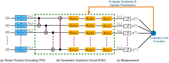
Figure 3: An illustration of the VQC model with three parts. (a) Tensor Product Encoding (TPE); (b) Parametric Quantum Circuit (PQC); (c) Measurement. The TPE employs a series of rotation gates $R_{Y}(\frac{\pi}{2}x_{i})$ to convert classical data into quantum states. The PQC consists of two-qubit CNOT gates and single-qubit rotation gates $R_{X}$, $R_{Y}$, $R_{Z}$ with trainable model parameters $\boldsymbol{\alpha}$, $\boldsymbol{\beta}$ and $\boldsymbol{\gamma}$. The CNOT gates impose the operation of quantum entanglement among qubits, and the gates $R_{X}$, $R_{Y}$, and $R_{Z}$ can be adjustable in the training stage. The PQC in the green dash square is repeatedly copied to generate a deeper PQC model. The measurement converts the quantum states $|z_{1}\rangle,|z_{2}\rangle,...,|z_{U}\rangle$ into the expectation values $\langle\sigma_{z}^{(1)}\rangle,\langle\sigma_{z}^{(2)}\rangle,...,\langle\sigma_{z}^{(U)}\rangle$ that are connected to a classified loss function. Moreover, an SGD algorithm is employed to update the VQC parameters.

The component of TPE was originally proposed in [44] and it converts a classical data x into a quantum state $|\textbf{x}\rangle$ by adopting a one-to-one mapping as:

$$|\textbf{x}\rangle=\left(\otimes_{i=1}^{U}R_{Y}(\frac{\pi}{2}x_{i})\right)|0\rangle^{\otimes U}=\begin{bmatrix}\cos(\frac{\pi}{2}x_{1})\\ \sin(\frac{\pi}{2}x_{1})\end{bmatrix}\otimes\begin{bmatrix}\cos(\frac{\pi}{2}x_{2})\\ \sin(\frac{\pi}{2}x_{2})\end{bmatrix}\otimes\cdot\cdot\cdot\otimes\begin{bmatrix}\cos(\frac{\pi}{2}x_{U})\\ \sin(\frac{\pi}{2}x_{U})\end{bmatrix},$$ (5)

where $\textbf{x}_{i}$ is strictly restricted in the domain of $[0,1]$ such that the conversion between x and $|\textbf{x}\rangle$ can be a reversely one-to-one mapping.

The PQC framework comprises $U$ quantum channels corresponding to accessible $U$ qubits on NISQ devices. We implement the quantum entanglement by using the controlled-NOT (CNOT) gates, and build up the PQC model based on single rotation gates $R_{X}$, $R_{Y}$, and $R_{Z}$ with adjustable parameters $\alpha=\{\alpha_{1},\alpha_{2},...,\alpha_{U}\}$, $\beta=\{\beta_{1},\beta_{2},...,\beta_{U}\}$, and $\gamma=\{\gamma_{1},\gamma_{2},...,\gamma_{U}\}$. The PQC model is associated with a linear operator that transforms the quantum input state $|\textbf{x}\rangle$ into the output $|\textbf{z}\rangle$. The PQC model in the green dashed square is repeatedly copied to set up a deeper structure. In this work, we set the depth of VQC as one for the consideration of the Barren Plateau problem.

The framework of measurement corresponds to the expectation of Hermitian operators based on Pauli-Z matrices, namely $\langle\sigma_{z}^{(1)}\rangle$, $\langle\sigma_{z}^{(2)}\rangle$, …, $\langle\sigma_{z}^{(U)}\rangle$, which results in the output vector $[\langle\sigma_{z}^{(1)}\rangle$, $\langle\sigma_{z}^{(2)}\rangle$, …, $\langle\sigma_{z}^{(U)}\rangle]^{T}$ followed by a softmax function for classification.

Next, we briefly introduce the TTN model. A TTN, also known as the matrix product state, refers to a tensor network with a 1-dimensional array and is formed by recursively employing singular value decomposition to a many-body wave function. More specifically, we first define the tensor-train decomposition on a 1-dimensional vector and a tensor-train representation for a 2-dimensional matrix. Specifically, given a vector $\textbf{x}\in\mathbb{R}^{D}$ where $D=\prod_{k=1}^{K}$, we reshape the vector x into a $K$-order tensor $\mathcal{X}\in\mathbb{R}^{D_{1}\times D_{2}\times\cdot\cdot\cdot\times D_{K}}$. Then, given a set of tensor-train ranks (TT-ranks) $\{R_{1},R_{2},...,R_{K+1}\}$ ($R_{1}$ and $R_{2}$ are set as $1$), all elements of $\mathcal{X}$ can be represented by multiplying $K$ matrices $\mathcal{X}_{d_{k}}^{[k]}$ as:

$$\mathcal{X}_{d_{1},d_{2},...,d_{K}}=\mathcal{X}_{d_{1}}^{[1]}\mathcal{X}_{d_{2}}^{[2]}\cdot\cdot\cdot\mathcal{X}_{d_{K}}^{[K]}=\prod\limits_{k=1}^{K}\mathcal{X}_{d_{k}}^{[k]},$$ (6)

where the matrices $\mathcal{X}_{d_{k}}^{[k]}\in\mathbb{R}^{R_{k}\times R_{k+1}},\forall d_{k}\in[D_{k}]$. The ranks $R_{1}$ and $R_{K+1}$ are set as $1$ to ensure the term $\prod_{k=1}^{K}\mathcal{X}_{d_{k}}^{[k]}$ to be a scalar.

Moreover, we consider the use of TTD for a 2-dimensional matrix. A feedforward neural network with $U$ neurons takes the form:

$$\text{y}(u)=\sum\limits_{d=1}^{D}\textbf{W}(d,u)\cdot\textbf{x}(d),\hskip 5.69054pt\forall u\in[U].$$ (7)

If $U=\sum_{k=1}^{K}u_{k}$ is assumed, we can reshape the $2$-dimensional matrix W as a $D$-order double-indexed tensor $\mathcal{W}$ and factorize it into the form as:

$$\mathcal{W}_{(d_{1},u_{1}),(d_{2},u_{2}),...,(d_{K},u_{K})}=\mathcal{W}_{d_{1},u_{1}}^{[1]}\mathcal{W}_{d_{2},u_{2}}^{[2]}\cdot\cdot\cdot\mathcal{W}_{d_{K},u_{K}}^{[K]}.$$ (8)

where $\mathcal{W}^{[k]}\in\mathbb{R}^{R_{k}\times D_{k}\times U_{k}\times R_{k+1}}$ is a $4$-order core tensor, and each $\mathcal{W}_{d_{k},u_{k}}^{[k]}\in\mathbb{R}^{R_{k}\times R_{k+1}}$ is a matrix. Accordingly, we can reshape the input vector x and the output one y into two tensors of the same order: $\mathcal{X}\in\mathbb{R}^{D_{1}\times D_{2}\times\cdot\cdot\cdot\times D_{K}}$, $\mathcal{Y}\in\mathbb{R}^{U_{1}\times U_{2}\times\cdot\cdot\cdot U_{K}}$, and we build the mapping function between the input $\mathcal{X}_{d_{1},d_{2},...,d_{K}}$ and the output one $\mathcal{Y}_{u_{1},u_{2},...,u_{K}}$ as:

$$\begin{split}\mathcal{Y}_{u_{1},u_{2},...,u_{K}}&=\sum\limits_{d_{1}=1}^{D_{1}}\sum\limits_{d_{2}=1}^{D_{2}}\cdot\cdot\cdot\sum\limits_{d_{K}=1}^{D_{K}}\mathcal{W}_{(d_{1},u_{1}),(d_{2},u_{2}),...(d_{K},u_{K})}\mathcal{X}_{d_{1},d_{2},...,d_{K}}\\ &=\sum\limits_{d_{1}=1}^{D_{1}}\sum\limits_{d_{2}=1}^{D_{2}}\cdot\cdot\cdot\sum\limits_{d_{K}=1}^{D_{K}}\prod\limits_{k=1}^{K}\mathcal{W}_{d_{k},u_{k}}^{[k]}\odot\prod\limits_{k=1}^{K}\mathcal{X}_{d_{k}}^{[k]}\\ &=\prod\limits_{k=1}^{K}\sum\limits_{d_{k}=1}^{D_{k}}\mathcal{W}_{d_{k},u_{k}}^{[k]}\odot\mathcal{X}_{d_{k}}^{[k]}\\ &=\prod\limits_{k=1}^{K}\mathcal{Y}_{u_{k}}^{[k]},\end{split}$$ (9)

where $\mathcal{W}_{d_{k},u_{k}}^{[k]}\odot\mathcal{X}_{d_{k}}^{[k]}$ is an element-wise multiplication of the two matrices, and $\sum_{d_{k}=1}^{D_{k}}\mathcal{W}_{d_{k},u_{k}}^{[k]}\odot\mathcal{X}_{d_{k}}^{[k]}$ leads to a matrix $\mathcal{Y}_{u_{k}}^{[k]}$ in $\mathbb{R}^{R_{k}\times R_{k+1}}$. The ranks $R_{1}=R_{K+1}=1$ ensures the term $\prod_{k=1}^{K}\mathcal{Y}_{u_{k}}^{[k]}$ is a scalar. Besides, a Sigmoid function is imposed upon each $\mathcal{Y}_{u_{1},u_{2},...,u_{K}}$, which generates a final output $\hat{\mathcal{Y}}$ with each element as:

$$\hat{\mathcal{Y}}_{u_{1},u_{2},...,u_{K}}=\text{Sigmoid}\left(\mathcal{Y}_{u_{1},u_{2},...,u_{K}}\right).$$ (10)

The benefits of utilizing the Sigmoid function have two folds: (1) it introduces a non-linearity to the quantum Hilbert space in the TPE stage; (2) making the TTN model become reversible such that for a TTN operator $\phi$, there exists a $\phi^{-1}$ such that $\phi\circ\phi^{-1}=1$.

2.2 Theoretical results

In this section, we first present the learning pipeline of Pre+TTN-VQC and then conduct its theoretical analysis in terms of upper bounding on each error component as shown in Eq. (2).

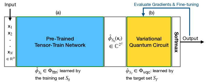
Figure 4: An illustration of the Pre+TTN-VQC architecture with a pre-trained TTN for feature abstraction and a VQC for classification. (a) Given the input vectors $\textbf{x}_{1},\textbf{x}_{2},...,\textbf{x}_{N}$ and the source dataset $S_{0}$, we obtain a pre-trained TTN $\hat{\phi}_{S_{0}}$ in the set of TTN operators $\Phi_{\rm ttn}$, which transforms the inputs $\textbf{x}_{i}$ into low-dimensional ones $\hat{\phi}_{S_{0}}(\textbf{x}_{i})$; (b) Given the set of VQC operators $\Phi_{\rm vqc}$, the VQC operator $\hat{\varphi}_{S_{T}}\in\Phi_{\rm vqc}$ is fine-tuned on a target dataset $S_{T}$, and then it is connected to the softmax operation to make predictions.

As illustrated in Figure 4, we first build up a generic TTN-VQC model based on the source dataset $S_{0}$. The well-trained TTN model of the generic TTN-VQC is then transferred to compose a Pre+TTN-VQC where the VQC is fine-tuned by using the target dataset $S_{T}$ but the pre-trained TTN is fixed and does not need further update any longer. Since the TTN admits a classical simulation of the quantum circuit with single and 2-qubit quantum gates on NISQ devices, both TTN-VQC and Pre+TTN-VQC are designed in end-to-end QNN pipelines.

Next, we characterize the Pre+TTN-VQC in terms of representation and generalization powers, and then we analyze the optimization performance of Pre+TTN-VQC by providing an upper bound without the PL condition. To exploit the theoretical error performance of Pre+TTN-VQC, we first analyze its representation power by upper bounding the representation error as shown in Theorem 1, and then we derive the upper bound on the estimation error for the related generalization power.

Theorem 1.

Given a smooth target operator $h_{\mathcal{D}}^{*}:\mathbb{R}^{Q}\rightarrow\mathbb{R}^{U}$ and $U$ qubits for the VQC, for a pre-trained TTN model $\hat{\phi}_{S_{0}}\in\Phi_{\rm ttn}$ conducted on the dataset $S_{0}$, we can find a VQC model $\rm\varphi\in\Phi_{\rm vqc}$ such that for a classified loss function $\mathcal{L}:\mathbb{R}^{U}\rightarrow\mathbb{R}$, there exists a TTN-VQC operator $f_{\mathcal{D}}^{*}$ satisfying

$$\epsilon_{\rm rep}=\mathcal{L}_{\mathcal{D}}(f_{\mathcal{D}}^{*})\leq 2\hat{\mathcal{R}}_{S_{0}}(\Phi_{\rm ttn})+\frac{1}{\sqrt{M}},$$ (11)

where $\hat{\mathcal{R}}_{S_{0}}(\Phi_{\rm ttn})$ refers to the empirical Rademacher complexity concerning the set $\Phi_{\rm ttn}$ on the given dataset $S_{0}$, $M$ is the count of measurement, and $\hat{\mathcal{R}}_{S_{0}}(\Phi_{\rm ttn})$ can be derived as:

$$\hat{\mathcal{R}}_{S_{0}}(\Phi_{\rm ttn})=\frac{2P}{\sqrt{|S_{0}|}}\sqrt{\sum\limits_{k=1}^{K}\Lambda_{k}^{2}},$$ (12)

where $P$ denotes the maximum power of input data, and each core tensor $\lVert\mathcal{W}^{[k]}\rVert_{F}\leq\Lambda_{k},\forall k\in[K]$.

Theorem 1 suggests that the upper bound on the representation error is composed of two terms: one is from the upper bound on the estimation error associated with the empirical Rademacher complexity of the pre-trained TTN, which is inversely proportional to $\sqrt{|S_{0}|}$; another one is related to the count of measurement. A larger dataset $S_{0}$ and more measurements of quantum output states are expected to lower the representation error of Pre+TTN-VQC.

In particular, compared with our previous work on the TTN-VQC, the number of qubits does not explicitly show up in the upper bound for the representation error, which results in two potential benefits from the TTN-VQC: (1) the pre-trained TTN architecture can alleviate the necessary condition to pursue a large number of qubits for boosting the representation power of VQC; (2) fewer qubits can be set to alleviate the Barren Plateau problem.

Theorem 2.

Based on the setup of Pre+TTN-VQC in Theorem 1, given the target dataset $S_{T}$, the estimation error is upper bounded by using the empirical Rademacher complexity $2\hat{\mathcal{R}}_{S_{T}}(\Phi_{\rm vqc})$ as:

$$\begin{split}&\hskip 5.69054pt\epsilon_{\rm est}\leq 2\hat{\mathcal{R}}_{S_{T}}(\Phi_{\rm vqc})\leq\frac{2P\Lambda}{\sqrt{|S_{T}|}},\\ &s.t.,\hskip 5.69054pt||\textbf{x}_{n}||_{2}\leq P,\hskip 2.84526pt\forall\textbf{x}_{n}\in S_{T},\hskip 2.84526pt\forall n\in[N]\\ &\hskip 22.76219pt||\textbf{W}_{\rm vqc}[:,u]||_{2}\leq\Lambda,\hskip 2.84526pt\forall u\in[U],\end{split}$$ (13)

where $\Phi_{\rm vqc}$ is the set of the VQC operators, $S_{T}$ denotes the given target dataset, and $P$ refers to the maximum power of encoded quantum states. Moreover, the unitary matrix $\textbf{W}_{\rm vqc}$ is associated with the VQC, and the $L_{2}$-norm of each column of $\textbf{W}_{\rm vqc}$ is upper bounded by a constant $\Lambda$.

We derive the upper bound on the estimation error $\epsilon_{\rm est}$ in Theorem 2. It suggests that given the pre-trained TTN, the estimation error of Pre+TTN-VQC is decided by the generalization capability of VQC that relies on the unitary matrix $\boldsymbol{W}_{\rm vqc}$. Given the constraints $P$ and $\Lambda$, we expect more target data in $S_{T}$ to lower the upper bound on the estimation error.

We make several assumptions to analyze the optimization performance to ensure an SGD can find a solution during the fine-tuning of VQC parameters on the target dataset $S_{T}$. Assumption 1 suggests two conditions of approximate linearity in fine-tuning and Assumption 2 refers to the constraint on the first-order gradient of VQC parameters.

Assumption 1 (Approximate linearity in fine-tuning).

Let $S_{T}=\{\textbf{x}_{1},\textbf{x}_{2},...,\textbf{x}_{|S_{T}|}\}$ be the set of target data. There exists a $f=\hat{\phi}_{S_{0}}\circ\varphi$ with a parameter $\theta$, denoted as $f(\textbf{x}_{n};\theta)$. Then, for two constants $\beta$, $L$ and a first-order gradient $\delta$, we have

$$\sup\limits_{\delta}\frac{1}{|S_{T}|}\sum\limits_{n=1}^{|S_{T}|}\left\lVert\nabla_{\theta}^{2}f(\textbf{x}_{n};\theta+\delta)\right\rVert_{2}^{2}\leq\beta^{2},$$ (14)

and

$$\sup\limits_{\theta}\frac{1}{|S_{T}|}\sum\limits_{n=1}^{|S_{T}|}\left\lVert\nabla_{\theta}f(\textbf{x}_{n};\theta)\right\rVert_{2}^{2}\leq L^{2}.$$ (15)

Assumption 2.

For the first-order gradient $\delta$ of VQC parameters during the fine-tuning process, we assume that $\sup_{\delta}\left\lVert\delta\right\rVert_{2}\leq R$ for a constant $R$.

Based on the above two Assumptions, we can further upper bound the optimization error $\epsilon_{\text{opt}}$ as shown in Theorem 3. The theoretical result of optimization performance shows that the upper bound on $\epsilon_{\text{opt}}$ is mainly controlled by the constraint factor $R$ for the supremum value of $\lVert\delta\rVert_{2}$. To lower the upper bound on $\epsilon_{\rm opt}$, a larger value $T_{\rm sgd}$ is expected, which corresponds to a very small learning rate $\eta$.

Theorem 3.

Given the constants $\beta$, $R$ and $L$ in Assumptions 1 and 2, for a total of $T_{\rm sgd}$ iterations with a learning rate $\eta$ as:

$$\eta=\frac{1}{\sqrt{T_{\rm sgd}}}\left(\frac{R}{\sqrt{L^{2}+\beta^{2}R^{2}}}\right),$$ (16)

we have

$$\epsilon_{\rm opt}\leq\beta R^{2}+R\sqrt{\frac{L^{2}+\beta^{2}R^{2}}{T_{\rm sgd}}}.$$ (17)

Compared with the Pre+TTN-VQC with a PL condition for lowering the optimization error, the pre-trained TTN architecture can guarantee that the Pre+TTN-VQC achieves a sufficiently low optimization error with a large iteration step $T_{\rm sgd}$ and a small upper bound $R$ for $\lVert\delta\rVert_{2}$.

To put it all together, with the constraint constants $\beta$, $R$ and $L$ defined in Assumption 1 and 2, the derived upper bounds on the error components can be combined into an aggregated one as:

$$\begin{split}\mathcal{L}_{\mathcal{D}}(\hat{f}_{S})&=\epsilon_{\rm rep}+\epsilon_{\rm est}+\epsilon_{\rm opt}\\ &\leq\frac{2P}{\sqrt{|S_{0}|}}\sqrt{\sum\limits_{k=1}^{K}\Lambda_{k}^{2}}+\frac{1}{\sqrt{M}}+\frac{2P\Lambda}{\sqrt{|S_{T}|}}+\beta R^{2}+R\sqrt{\frac{L^{2}+\beta^{2}R^{2}}{T_{\rm sgd}}}\\ s.t.,\hskip 2.84526pt&\lVert\textbf{x}_{n}\rVert_{2}\leq P,\hskip 2.84526pt\forall\textbf{x}_{n}\in S_{T},\forall n\in[N],\\ &||\boldsymbol{W}_{\text{vqc}}[:,u]||_{2}\leq\Lambda,\hskip 2.84526pt\forall u\in[U],\\ &\lVert\mathcal{W}^{[k]}\rVert_{F}\leq\Lambda_{k},\hskip 2.84526pt\forall k\in[K].\end{split}$$ (18)

Our theoretical result suggests that both larger $|S_{0}|$ and $|S_{T}|$ can lower the aggregated upper bound, but we expect not so much target data in $S_{T}$ for the fine-tuning of VQC parameters.

2.3 Empirical results

To corroborate our theoretical results of the Pre+TTN-VQC, our experimental simulations are divided into two groups: (1) to assess the representation power of Pre+TTN-VQC, both the training and test datasets are set in the same clean environment; (2) to evaluate the generalization power of Pre+TTN-VQC, the training data are put in a clean environment but the test data are mixed with additive Gaussian noise. Moreover, the training data comprise a source dataset $S_{0}$ for training the Pre+TTN-VQC and a target dataset $S_{T}$ for fine-tuning the VQC, where there is no overlapping between $S_{0}$ and $S_{T}$. The test data share the same classified labels as the target ones but are not included in $S_{T}$. Our experimental results compare the performance of Pre+TTN-VQC with the baseline results of the TTN-VQC and PCA-VQC counterparts that have been discussed in [37, 36]. In particular, this work aims at verifying the following points:

1. The Pre+TTN-VQC with a pre-trained TTN can lead to better performance than the TTN-VQC and PCA-VQC counterparts in both matched and unmatched environmental conditions.

2. More source data in $S_{0}$ improves the representation power, and increasing the amount of target data in $S_{T}$ can lead to better generalization power.

3. The setting of pre-trained TTN for TTN-VQC ensures exponential convergence rates.

In this work, we assess the performance of Pre+TTN-VQC on the standard MNIST dataset [13]. The dataset focuses on the task of handwritten $10$ digit classification, where $60,000$ training data and $10,000$ test data are included. We randomly collect $18,000$ training data of six digits $\{1,2,3,4,5,6\}$ to include in the source dataset $S_{0}$ and assign another $2000$ training data of two digits $\{2,5\}$ to constitute the target dataset $S_{T}$. Accordingly, the test dataset comprises all the test data of digits $\{2,5\}$, which are not seen in the datasets $S_{0}$ and $S_{T}$.

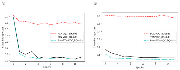
Figure 5: Experiments on the MNIST dataset to assess the representation power of Pre+TTN-VQC. a empirical results on the training data. b empirical results on the test data. PCA-VQC$\_$8Qubit represents the PCA-VQC model with $8$ qubits; TTN-VQC$\_$8Qubits and Pre+TTN-VQC$\_$8Qubits separately refer to the TTN-VQC and Pre+TTN-VQC models with $8$ qubits.

As for the setups of Pre+TTN-VQC and TTN-VQC, the image data are reshaped into a $3$-order $7\times 16\times 7$ tensors. Given the TT-ranks $\{1,3,3,1\}$, we can set $3$ trainable tensors as: $\mathcal{W}_{1}\in\mathbb{R}^{1\times 7\times U_{1}\times 3}$, $\mathcal{W}_{2}\in\mathbb{R}^{3\times 16\times U_{2}\times 3}$, and $\mathcal{W}_{3}\in\mathbb{R}^{3\times 7\times U_{3}\times 1}$, where $U=\prod_{k=1}^{3}U_{k}$ stands for the number of qubits. Particularly, we evaluate the models with $8$ qubits and the parameters $(U_{1},U_{2},U_{3})$ are set as $(2,2,2)$ associated with the $8$ qubits. The SGD with an Adam optimizer is employed in the training process in which a mini-batch of $50$ and a learning rate of $0.001$ are configured. Besides, we compare the Pre+TTN-VQC with the previously proposed PCA-VQC and TTN-VQC as the baseline models. The TTN-VQC follows an end-to-end learning paradigm in Figure 1 (a) without the pre-training procedure, and PCA-VQC takes PCA for the feature dimensionality followed by the VQC as a classifier. Moreover, both the training data $S_{0}$ and $S_{T}$ are employed for the training of PCA-VQC and TTN-VQC. The cross-entropy (CE) [12] is chosen as the loss function in the training process, and the experimental setups for PCA-VQC and TTN-VQC are consistent with our previous work [37].

The training and test data are kept in a clean environment to corroborate Theorem 1 for the representation power of Pre+TTN-VQC. Figure 5 shows the related empirical results, where PCA-VQC$\_$8Qubits denotes the PCA for feature dimensionality followed by the VQC as a classifier with $8$ qubits, and Pre+TTN-VQC$\_$8Qubits and TTN-VQC$\_$8Qubits separately correspond to the Pre+TTN-VQC and TTN-VQC models with $8$ qubits. Our experiments show that both TTN-VQC and Pre+TTN-VQC can get converged to low CE values but the PCA-VQC cannot decrease the CE loss to a small scale because of the Barren Plateau landscape. Moreover, Table 2 presents the final experimental results of the related models on the test dataset. Both Pre+TTN-VQC and TTN-VQC own more parameters than PCA-VQC, but the former achieves much lower CE scores and higher accuracies. Moreover, the Pre+TTN-VQC attains even better empirical performance than the TTN-VQC with a lower CE score (0.0390 vs. 0.0625) and a higher accuracy ($99.0\%$ vs. $98.7\%$).

The experimental results demonstrate that the PCA-VQC suffers from a serious Barren Plateau problem and cannot find a good minimal point, but both TTN-VQC and Pre+TTN-VQC can finally converge to minima with low CE scores. The TTN-VQC assumes a PL condition in [37], but Pre+TTN-VQC follows the pre-trained setup discussed in this work. Besides, the Pre+TTN-VQC also performs faster convergence rates than the TTN-VQC counterpart and achieves much lower CE scores and higher accuracies, which corroborate our theorem that the setup of the pre-trained TTN can easily overcome the Barren Plateau landscape for the VQC.

Table 2: Empirical results of Pre+TTN-VQC, TTN-VQC, and PCA-VQC models on the test dataset to assess the generalization power.

Models	Params (Mb)	CE	Accuracy ($\%$)
PCA-VQC$\_8$Qubit	0.080	0.5744	75.8
TTN-VQC$\_8$Qubit	0.452	0.0625	98.7
Pre+TTN-VQC$\_8$Qubit	0.452	0.0390	99.0

Furthermore, we incrementally increase the amount of training data in $S_{0}$ and the related experimental results are shown in Table 3. The results show that the experimental performance of Pre+TTN-VQC can become better with the increase of the amount of training data in $S_{0}$, which justifies our theoretical result in Theorem 1 that larger data size in $S_{0}$ correspond to a lower upper bound on the representation error.

Table 3: Empirical results of the Pre+TTN-VQC on the source dataset of different amounts of data in $S_{0}$.

Models	$\#$ Data in $S_{0}$	CE	Accuracy ($\%$)
Pre+TTN-VQC$\_8$Qubit	18,000	0.0390	99.0
Pre+TTN-VQC$\_8$Qubit	24,000	0.0347	99.1
Pre+TTN-VQC$\_8$Qubit	30,000	0.0321	99.3

To assess the generalization power of Pre+TTN-VQC, we separately mix the test data with additive Gaussian and Laplacian noises with $6$dB levels. Based on the well-trained models of Pre+TTN-VQC, TTN-VQC, and PCA-VQC, we assess their performance on the noisy test datasets related to the evaluation of their generalization power. For one thing, Figure 6 suggests that both Pre+TTN-VQC and TTN-VQC outperform the PCA-VQC counterpart on the test dataset of the two unmatched noisy settings. In particular, the Pre+TTN-VQC attains even better empirical results regarding faster convergence rates, lower CE scores, and higher accuracies on the test datasets of the two noisy settings. Especially, in the more adverse Laplacian noisy setting, the performance gain of Pre+TTN-VQC becomes more outstanding. The empirical results corroborate the Theorem 2 that the pre-training can also improve the experimental performance of TTN-VQC without the assumption of PL condition.

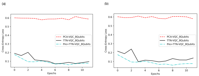
Figure 6: Experiments on the MNIST dataset mixed with noises to assess the generalization power of Pre+TTN-VQC. a empirical results on the test data with the Gaussian noise of 6dB. b empirical results on the test data with the Laplacian noise of 6dB. PCA-VQC$\_$8Qubit represents the PCA-VQC model with $8$ qubits; TTN-VQC$\_$8Qubits and Pre+TTN-VQC$\_$8Qubits separately refer to the TTN-VQC and Pre+TTN-VQC models with $8$ qubits.

Table 4: Empirical results of Pre+TTN-VQC on the noisy test dataset to assess the generalization power.

Models	Noise type	Params (Mb)	CE	Accuracy ($\%$)
PCA-VQC$\_$8Qubit	Gaussian (6dB)	0.080	0.5868	72.5
PCA-VQC$\_$8Qubit	Laplacian (6dB)	0.080	0.5791	72.6
TTN-VQC$\_$8Qubit	Gaussian (6dB)	0.452	0.0943	97.8
TTN-VQC$\_$8Qubit	Laplacian (6dB)	0.452	0.1395	96.3
Pre+TTN-VQC$\_$8Qubit	Gaussian (6dB)	0.452	0.0769	98.5
Pre+TTN-VQC$\_$8Qubit	Laplacian (6dB)	0.452	0.1160	97.2

Besides, we observe the related experimental performance by increasing the amount of target data in $S_{T}$. The results in Table 5 show that with the increase of the amount of target data in $S_{T}$, the Pre+TTN-VQC can consistently attain lower CE scores and higher accuracies, which corroborate the Theorem 2 that more target data in $S_{T}$ lead to a lower upper bound on the estimation error.

Table 5: Empirical results of the Pre+TTN-VQC on the target dataset of different amounts of data in $S_{T}$.

Models	Noise type	$\#$ Data in $S_{T}$	CE	Accuracy ($\%$)
Pre+TTN-VQC$\_8$Qubit	Laplacian (6dB)	2,000	0.1160	97.2
Pre+TTN-VQC$\_8$Qubit	Laplacian (6dB)	2,500	0.1103	97.3
Pre+TTN-VQC$\_8$Qubit	Laplacian (6dB)	3,000	0.1056	97.5

3 DISCUSSION

This work mainly discusses the benefits of pre-training of TTN for the setup of TTN-VQC to overcome the Barren Plateau problem. We first leverage the theoretical error performance analysis to derive upper bounds on the representation error, estimation error, and optimization errors for the Pre+TTN-VQC. Our theoretical results suggest that the representation error is inversely proportional to the square root of the amount of data in the source dataset, which implies that more pre-trained data could benefit the representation power of TTN-VQC. The estimation error of Pre+TTN-VQC is related to the generalization power associated with an upper bound on the empirical Rademacher complexity, where more data in the target dataset can contribute better generalization capability. The optimization error can be reduced to a small score by employing the pre-trained setup for TTN followed by the VQC fine-tuning based on the SGD algorithm. To our best knowledge, no prior works have been delivered, such as the pre-trained TTN for VQC and the related theoretical characterization.

We conduct experiments on the MNIST dataset to verify our theoretical results. To highlight better representation and generalization powers of Pre+TTN-VQC, we compare the experimental performance of the Pre+TTN-VQC with the TTN-VQC and PCA-VQC counterparts. Without the setup of PL condition for TTN-VQC, the pre-trained TTN can overcome the Barren Plateau problem and achieve even better empirical results under both matched and unmatched noisy scenarios. In particular, our experimental simulation demonstrates that increasing data amounts in the source dataset leads to better representation power; In the meanwhile, assigning more data to the target dataset results in better generalization performance. We also note that the Pre+TTN-VQC attains faster exponential convergence rates and higher accuracies than the TTN-VQC, making the Pre+TTN-VQC a better choice for the TTN-VQC to handle the Barren Plateau landscape.

Furthermore, our theoretical and empirical results are built upon the fact that no data distribution shift exists between the source dataset and the target one. It means that the source dataset should cover more scenarios in the target dataset, and the pre-trained TTN setting may not work if there is no overlapping between the two datasets. Our future work aims at new quantum optimization algorithms to deal with the potential problem of the data distribution shift.

4 METHONDS

This section aims to provide proof of our theoretical results. More specifically, we separately prove the upper bound for the representation error, estimation error, and optimization bias.

4.1 Proof of Theorem 1

Given the target function $h_{\mathcal{D}}^{*}$, and two Pre+TTN-VQC hypotheses $f_{\mathcal{D}}^{*}=\phi^{*}_{\mathcal{D}}\circ\varphi_{\mathcal{D}}^{*}$ and $f_{S_{0}}^{*}=\hat{\phi}_{S_{0}}\circ\varphi_{\mathcal{D}}^{*}$ in which $\hat{\phi}_{S_{0}}$ is an empirical Pre+TTN, we have

$$\begin{split}\mathcal{L}_{\mathcal{D}}(f_{\mathcal{D}}^{*})&=\mathcal{L}_{\mathcal{D}}(f_{S_{0}}^{*})+\mathcal{L}_{\mathcal{D}}(f_{\mathcal{D}}^{*})-\mathcal{L}_{\mathcal{D}}(f_{S_{0}}^{*})\\ &=\mathcal{L}_{\mathcal{D}}(\hat{\phi}_{S_{0}}\circ\varphi_{\mathcal{D}}^{*})+\left(\mathcal{L}_{\mathcal{D}}(\phi^{*}_{\mathcal{D}}\circ\varphi_{\mathcal{D}}^{*})-\mathcal{L}_{\mathcal{D}}(\hat{\phi}_{S_{0}}\circ\varphi_{\mathcal{D}}^{*})\right).\end{split}$$ (19)

Then, we separately upper bound the above two terms $\mathcal{L}_{\mathcal{D}}(\hat{\phi}_{S_{0}}\circ\varphi_{\mathcal{D}}^{*})$ and $\mathcal{L}_{\mathcal{D}}(\phi^{*}_{\mathcal{D}}\circ\varphi_{\mathcal{D}}^{*})-\mathcal{L}_{\mathcal{D}}(\hat{\phi}_{S_{0}}\circ\varphi_{\mathcal{D}}^{*})$ as follows:

• As for the first term, for a given pre-trained TTN operator $\hat{\phi}_{S_{0}}$, based on our analysis of TTN in the preliminary results, there exists a $\hat{\phi}^{-1}_{S_{0}}$ such that $h_{\mathcal{D}}^{*}=\hat{\phi}_{S_{0}}\circ\hat{\phi}_{S_{0}}^{-1}\circ h_{\mathcal{D}}^{*}$. Then, the representation error comes from the approximation bias between $\varphi_{\mathcal{D}}^{*}$ and $\hat{\phi}_{S_{0}}^{-1}\circ h_{\mathcal{D}}^{*}$, which is upper bounded by $\mathcal{O}(\frac{1}{\sqrt{M}})$ based on the universal approximation property of quantum neural networks [20].

  $$\begin{split}\mathcal{L}_{\mathcal{D}}(\hat{\phi}_{S_{0}}\circ\varphi_{\mathcal{D}}^{*})&=\mathcal{L}_{\mathcal{D}}(\hat{\phi}_{S_{0}}\circ\varphi_{\mathcal{D}}^{*},h_{\mathcal{D}}^{*})\\ &=\mathcal{L}_{\mathcal{D}}(\hat{\phi}_{S_{0}}\circ\varphi_{\mathcal{D}}^{*},\hat{\phi}_{S_{0}}\circ(\hat{\phi}_{S_{0}}^{-1}\circ h_{\mathcal{D}}^{*}))\\ &\leq\mathcal{O}\left(\frac{1}{\sqrt{M}}\right).\end{split}$$ (20)

• For the second term, given the optimal hypothesis $\phi^{*}_{\mathcal{D}}$, the second term corresponds to the estimation error of the TTN model on the dataset $S_{0}$. Based on our previous theory in [35], this term can be upper bounded as:

  $$\mathcal{L}_{\mathcal{D}}(\phi^{*}_{\mathcal{D}}\circ\varphi_{\mathcal{D}}^{*})-\mathcal{L}_{\mathcal{D}}(\hat{\phi}_{S_{0}}\circ\varphi_{\mathcal{D}}^{*})\leq 2\hat{\mathcal{R}}_{S_{0}}(\Phi_{\rm ttn}),$$ (21)

  where $\hat{\mathcal{R}}_{S_{0}}(\Phi_{\rm ttn})$ represents an empirical Rademacher complexity for the TTN functional set. For a $\phi\in\Phi_{\rm ttn}$, we define the empirical Rademacher complexity of TTN as:

  $$\begin{split}\hat{\mathcal{R}}_{S_{0}}(\Phi_{\text{ttn}})&=\frac{1}{|S_{0}|}\mathbb{E}_{\boldsymbol{\sigma}}\left[\sup\limits_{\phi\in\Phi_{\text{ttn}}}\sum\limits_{n=1}^{|S_{0}|}\sigma_{n}\phi(\textbf{x}_{n})\right]=\frac{2P}{\sqrt{|S_{0}|}}\sqrt{\sum_{k=1}^{K}\Lambda_{k}}\\ &s.t.,\hskip 2.84526pt\lVert\mathcal{W}^{[k]}\rVert_{F}\leq\Lambda_{k},\forall k\in[K],\end{split}$$ (22)

  where the random variables $\sigma_{i}$ are called Rademacher variables taking values in $\{-1,1\}$ and the final derived upper bound on $\hat{\mathcal{R}}_{S_{0}}(\Phi_{\rm ttn})$ comes from Theorem 2 in our previous work [37].

4.2 Proof of Theorem 2

Given a target dataset $S_{T}=\{\textbf{x}_{1},\textbf{x}_{2},...,\textbf{x}_{T}\}$ and $U$ qubits for the VQC, based on the mathematical setups in Eq. (2), we have

$$\begin{split}\epsilon_{\text{est}}&=\mathcal{L}_{\mathcal{D}}(f_{S_{T}}^{*})-\mathcal{L}_{\mathcal{D}}(f_{\mathcal{D}}^{*})\\ &=\mathcal{L}_{\mathcal{D}}(\hat{\phi}_{S_{0}}\circ\varphi_{S_{T}}^{*})-\mathcal{L}_{\mathcal{D}}(\hat{\phi}_{S_{0}}\circ\varphi_{\mathcal{D}}^{*})\\ &\rm\leq 2\hat{\mathcal{R}}_{S_{T}}(\Phi_{\rm vqc}),\end{split}$$ (23)

where $\hat{\mathcal{R}}_{S_{T}}(\Phi_{\rm vqc})$ represents the empirical Rademacher complexity for the VQC functional set. Then, we upper bound $\hat{\mathcal{R}}_{S_{T}}(\Phi_{\rm vqc})$ using the definition as:

$$\begin{split}\hat{\mathcal{R}}_{S_{T}}(\Phi_{\text{vqc}})&=\frac{1}{|S_{T}|}\mathbb{E}_{\boldsymbol{\sigma}}\left[\sup\limits_{\lVert\textbf{w}_{u}\rVert_{2}\leq\Lambda}\sum\limits_{n=1}^{|S_{T}|}\sigma_{n}\sum\limits_{u=1}^{U}\textbf{w}_{u}\cdot\textbf{x}_{n}\right]\\ &=\frac{1}{|S_{T}|}\mathbb{E}_{\boldsymbol{\sigma}}\left[\sup\limits_{\lVert\textbf{w}_{u}\rVert_{2}\leq\Lambda}\sup\limits_{s\in\{-1,1\}}s\sum\limits_{n=1}^{|S_{T}|}\sigma_{n}\textbf{w}_{u}\cdot\textbf{x}_{n}\right]\\ &=\frac{1}{|S_{T}|}\mathbb{E}_{\boldsymbol{\sigma}}\left[\sup\limits_{\lVert\textbf{w}\rVert_{2}\leq\Lambda,u\in[1,U]}\left|\textbf{w}_{u}\cdot\sum\limits_{n=1}^{|S_{T}|}\sigma_{n}\textbf{x}_{n}\right|\right]\\ &=\frac{\Lambda}{|S_{T}|}\mathbb{E}_{\boldsymbol{\sigma}}\left[\left\lVert\sum\limits_{n=1}^{|S_{T}|}\sigma_{n}\textbf{x}_{n}\right\rVert_{2}\right]\\ &\leq\frac{\Lambda}{|S_{T}|}\sqrt{\mathbb{E}_{\boldsymbol{\sigma}}\left[\left\lVert\sum\limits_{n=1}^{|S_{T}|}\sigma_{n}\textbf{x}_{n}\right\rVert_{2}^{2}\right]}\hskip 14.22636pt(\text{Jensen's inequality})\\ &=\frac{\Lambda}{|S_{T}|}\sqrt{\sum\limits_{i,j=1}^{|S_{T}|}\mathbb{E}_{\boldsymbol{\sigma}}[\sigma_{i}\sigma_{j}]\left(\textbf{x}_{i}\cdot\textbf{x}_{j}\right)}.\end{split}$$ (24)

Since $\sigma_{i}$ are identically and independently distributed, we have

$$\mathbb{E}_{\boldsymbol{\sigma}}[\sigma_{i}\sigma_{j}]=\begin{cases}\hskip 7.11317pt1,\hskip 8.53581pt\text{if $i=j$}\\ -1,\hskip 8.53581pt\text{if $i\neq j$}.\end{cases}$$ (25)

Then, we can upper bound the $\hat{\mathcal{R}}_{S_{T}}(\Phi_{\rm vqc})$ as:

$$\begin{split}\hat{\mathcal{R}}_{S_{T}}(\Phi_{\text{vqc}})&\leq\frac{\Lambda}{|S_{T}|}\sqrt{\sum\limits_{i,j=1}^{|S_{T}|}1_{i=j}(\textbf{x}_{i}\cdot\textbf{x}_{j})}\\ &=\frac{\Lambda}{|S_{T}|}\sqrt{\sum\limits_{n=1}^{|S_{T}|}\lVert\textbf{x}_{n}\rVert_{2}^{2}}\hskip 51.21495pt(\lVert\textbf{x}_{n}\rVert_{2}^{2}\leq P^{2})\\ &\leq\frac{\Lambda P}{\sqrt{|S_{T}|}}.\end{split}$$ (26)

4.3 Proof of Theorem 3

Given the target dataset $S_{T}=\{\textbf{x}_{1},\textbf{x}_{2},...,\textbf{x}_{N}\}$, we associate the VQC parameters $\hat{\theta}$ and $\theta^{*}$ in $\Theta$ with $\hat{f}_{S_{T}}$ and $f_{S_{T}}^{*}$. Moreover, we employ the empirical loss function $\mathcal{L}_{S}(\cdot)$ to approximate the expected loss function $\mathcal{L}_{\mathcal{D}}(\cdot)$. For simplicity, we define $\mathcal{L}_{\mathcal{S}}(\hat{\theta})=\mathcal{L}_{\mathcal{S}}(\hat{f}_{S_{T}})$ and $\mathcal{L}_{S}(\theta^{*})=\mathcal{L}_{S}(f_{S_{T}}^{*})$. At the iteration $t$ of the SGD algorithm, we focus on the updated parameter $\theta_{t}$ and the related $\mathcal{L}_{S}(\theta_{t})$. For any $t\in[T_{\rm sgd}]$, we have

$$\begin{split}r_{t+1}^{2}&=\lVert\theta_{t+1}-\theta^{*}\rVert_{2}^{2}\\ &\leq\lVert\theta_{t}-\eta\nabla\mathcal{L}_{S}(\theta_{t})-\theta^{*}\rVert_{2}^{2}\\ &=r_{t}^{2}+2\eta\langle\nabla_{\theta}\mathcal{L}_{S}(\theta_{t}),\theta^{*}-\theta_{t}\rangle+\eta^{2}\lVert\nabla_{\theta}\mathcal{L}_{S}(\theta_{t})\rVert_{2}^{2}.\end{split}$$ (27)

To further upper bound $r_{t+1}^{2}$, we separately derive upper bounds on the terms $\langle\nabla_{\theta}\mathcal{L}(\theta_{t}),\theta^{*}-\theta_{t}\rangle$ and $\lVert\nabla_{\theta}\mathcal{L}(\theta_{t})\rVert_{2}^{2}$ with Assumption 1 and Assumption 2.

• To upper bound the term $\langle\nabla_{\theta}\mathcal{L}_{S}(\theta_{t}),\theta^{*}-\theta_{t}\rangle$, we are based on the theory of approximate convexity [6], which is presented in Lemma 4.

  Lemma 4 (Approximate convexity in $\Theta$).

  Let $\theta_{1},\theta_{2}\in\Theta$. Then,

  $$\langle\nabla_{\theta}\mathcal{L}_{S}(\theta_{1}),\theta_{2}-\theta_{1}\rangle\leq\mathcal{L}_{S}(\theta_{2})-\mathcal{L}_{S}(\theta_{1})+4\beta R^{2}.$$ (28)

• To upper bound the term $\lVert\nabla_{\theta}\mathcal{L}_{S}(\theta_{t})\rVert_{2}^{2}$, we employ the property of gradient bound [6], which is shown in Lemma 5.

  Lemma 5 (Gradient bound in $\Theta$).

  For any $\theta\in\Theta$, we have that

  $$\lVert\nabla_{\theta}\mathcal{L}_{S}(\theta)\rVert_{2}^{2}\lesssim L^{2}+\beta^{2}R^{2}.$$ (29)

Thus, based on Lemma 4 and Lemma 5, we can leverage the telescoping technique [30] to further upper bound $r_{t+1}^{2}$ as:

$$\begin{split}r_{t+1}^{2}&\leq r_{t}^{2}+2\eta\left(\mathcal{L}(\theta^{*})-\mathcal{L}(\theta_{t})+4\beta R^{2}\right)+\eta^{2}(L^{2}+\beta^{2}R^{2})\\ &\leq r_{0}^{2}+2\eta\left(\sum\limits_{t=0}^{T_{\rm sgd}-1}\mathcal{L}_{S}(\theta^{*})-\mathcal{L}_{S}(\theta_{t})\right)+8\eta T_{\rm sgd}\beta R^{2}+\eta^{2}T_{\rm sgd}(L^{2}+\beta^{2}R^{2}).\end{split}$$ (30)

By rearranging the last inequality, we have

$$\begin{split}\frac{r_{0}^{2}-r^{2}_{T_{\rm sgd}}}{2\eta T_{\rm sgd}}+4\beta R^{2}+\frac{\eta}{2}(L^{2}+\beta^{2}R^{2})&\geq\frac{1}{T_{\rm sgd}}\sum\limits_{t=0}^{T_{\rm sgd}-1}\mathcal{L}_{S}(\theta^{*})-\mathcal{L}(\theta_{t})\\ &\geq\min\limits_{t=0,...,T_{\rm sgd}-1}\mathcal{L}(\theta^{*})-\mathcal{L}(\theta_{t}).\end{split}$$ (31)

Now, using the step size $\eta=\frac{1}{\sqrt{T_{\rm sgd}}}(\frac{R}{\sqrt{L^{2}+\beta^{2}R^{2}}})$, we observe that

$$\begin{split}\frac{r_{0}^{2}-r^{2}_{T_{\rm sgd}}}{2\eta T_{\rm sgd}}+\frac{\eta}{2}(L^{2}+\beta^{2}R^{2})&\leq\frac{R^{2}}{2\eta T_{\rm sgd}}+\frac{\eta}{2}(L^{2}+\beta^{2}R^{2})\\ &=R\sqrt{\frac{L^{2}+\beta^{2}R^{2}}{T_{\rm sgd}}},\end{split}$$ (32)

from which the upper bound for the optimization error in Theorem 3 follows.

References

- Abbas et al. [2021] Abbas, Amira, Sutter, David, Zoufal, Christa, Lucchi, Aurélien, Figalli, Alessio, and Woerner, Stefan. The Power of Quantum Neural Networks. Nature Computational Science, 1(6):403–409, 2021.
- Beer et al. [2020] Beer, Kerstin et al. Training Deep Quantum Neural Networks. Nature Communications, 11(1):808, 2020.
- Benedetti et al. [2019] Benedetti, Marcello, Lloyd, Erika, Sack, Stefan, and Fiorentini, Mattia. Parameterized Quantum Circuits as Machine Learning Models. Quantum Science and Technology, 4(4):043001, 2019.
- Biamonte et al. [2017] Biamonte, Jacob, Wittek, Peter, Pancotti, Nicola, Rebentrost, Patrick, Wiebe, Nathan, and Lloyd, Seth. Quantum Machine Learning. Nature, 549(7671):195–202, 2017.
- Brown et al. [2020] Brown, Tom et al. Language Models Are Few-Shot Learners. In Advances in Neural Information Processing Systems, volume 33, pp. 1877–1901, 2020.
- Bubeck [2015] Bubeck, Sébastien. Convex Optimization: Algorithms and Complexity. Foundations and Trends in Machine Learning, 8(3-4):231–357, 2015.
- Caro et al. [2022] Caro, Matthias C et al. Generalization In Quantum Machine Learning From Few Training Data. Nature Communications, 13(1):4919, 2022.
- Cerezo et al. [2022] Cerezo, M, Verdon, Guillaume, Huang, Hsin-Yuan, Cincio, Lukasz, and Coles, Patrick J. Challenges and opportunities in quantum machine learning. Nature Computational Science, 2(9):567–576, 2022.
- Cerezo et al. [2021] Cerezo, Marco et al. Variational Quantum Algorithms. Nature Reviews Physics, 3(9):625–644, 2021.
- Chen et al. [2020] Chen, Samuel Yen-Chi, Yang, Chao-Han Huck, Qi, Jun, Chen, Pin-Yu, Ma, Xiaoli, and Goan, Hsi-Sheng. Variational Quantum Circuits for Deep Reinforcement Learning. IEEE Access, 8:141007–141024, 2020.
- Cong et al. [2019] Cong, Iris, Choi, Soonwon, and Lukin, Mikhail D. Quantum Convolutional Neural Networks. Nature Physics, 15(12):1273–1278, 2019.
- De Boer et al. [2005] De Boer, Pieter-Tjerk, Kroese, Dirk P, Mannor, Shie, and Rubinstein, Reuven Y. A Tutorial on the Cross-Entropy Method. Annals of Operations Research, 134:19–67, 2005.
- Deng [2012] Deng, Li. The MNIST Database of Handwritten Digit Images for Machine Learning Research. IEEE Signal Processing Magazine, 29(6):141–142, 2012.
- Du et al. [2020] Du, Yuxuan, Hsieh, Min-Hsiu, Liu, Tongliang, and Tao, Dacheng. Expressive Power of Parametrized Quantum Circuits. Physical Review Research, 2(3):033125, 2020.
- Du et al. [2021] Du, Yuxuan, Hsieh, Min-Hsiu, Liu, Tongliang, You, Shan, and Tao, Dacheng. Learnability of Quantum Neural Networks. PRX Quantum, 2(4):040337, 2021.
- Dunjko [2022] Dunjko, Vedran. Quantum Learning Unravels Quantum System. Science, 376(6598):1154–1155, 2022.
- Egan et al. [2021] Egan, Laird et al. Fault-tolerant Control of An Error-Corrected Qubit. Nature, 598(7880):281–286, 2021.
- Fang et al. [2020] Fang, Tongtong, Lu, Nan, Niu, Gang, and Sugiyama, Masashi. Rethinking importance weighting for deep learning under distribution shift. In Advances in Neural Information Processing Systems, volume 33, pp. 11996–12007, 2020.
- Floridi & Chiriatti [2020] Floridi, Luciano and Chiriatti, Massimo. GPT-3: Its Nature, Scope, Limits, and Consequences. Minds and Machines, 30:681–694, 2020.
- Goto et al. [2021] Goto, Takahiro, Tran, Quoc Hoan, and Nakajima, Kohei. Universal Approximation Property of Quantum Machine Learning Models in Quantum-Enhanced Feature Spaces. Physical Review Letters, 127(9):090506, 2021.
- Huang et al. [2021] Huang, He-Liang et al. Experimental Quantum Generative Adversarial Networks for Image Generation. Physical Review Applied, 16(2):024051, 2021.
- Huembeli & Dauphin [2021] Huembeli, Patrick and Dauphin, Alexandre. Characterizing the Loss Landscape of Variational Quantum Circuits. Quantum Science and Technology, 6(2):025011, 2021.
- Karimi et al. [2016] Karimi, Hamed, Nutini, Julie, and Schmidt, Mark. Linear Convergence of Gradient and Proximal-Gradient Methods Under the Polyak-Łojasiewicz Condition. In Joint European Conference on Machine Learning and Knowledge Discovery in Databases, pp. 795–811. Springer, 2016.
- Kingma & Ba [2015] Kingma, Diederik P and Ba, Jimmy. Adam: A Method for Stochastic Optimization. In International Conference on Learning Representation, 2015.
- Liang et al. [2022] Liang, Zhiding et al. Variational Quantum Pulse Learning. In IEEE International Conference on Quantum Computing and Engineering, pp. 556–565, 2022.
- Liu et al. [2021] Liu, Yunchao, Arunachalam, Srinivasan, and Temme, Kristan. A Rigorous and Robust Quantum Speed-up in Supervised Machine Learning. Nature Physics, 17(9):1013–1017, 2021.
- Mari et al. [2020] Mari, Andrea, Bromley, Thomas R, Izaac, Josh, Schuld, Maria, and Killoran, Nathan. Transfer Learning in Hybrid Classical-Quantum Neural Networks. Quantum, 4:340, 2020.
- McClean et al. [2018] McClean, Jarrod R, Boixo, Sergio, Smelyanskiy, Vadim N, Babbush, Ryan, and Neven, Hartmut. Barren Plateaus in Quantum Neural Network Training Landscapes. Nature Communications, 9(1):1–6, 2018.
- Mitarai et al. [2018] Mitarai, Kosuke, Negoro, Makoto, Kitagawa, Masahiro, and Fujii, Keisuke. Quantum Circuit Learning. Physical Review A, 98(3):032309, 2018.
- Mohri et al. [2018] Mohri, Mehryar, Rostamizadeh, Afshin, and Talwalkar, Ameet. Foundations of Machine Learning. 2018.
- Noormandipour & Wang [2022] Noormandipour, Mohammadreza and Wang, Hanchen. Matching Point Sets with Quantum Circuit Learning. In IEEE International Conference on Acoustics, Speech and Signal Processing, pp. 8607–8611, 2022.
- Oseledets [2011] Oseledets, Ivan V. Tensor-Train Decomposition. SIAM Journal on Scientific Computing, 33(5):2295–2317, 2011.
- Preskill [2018] Preskill, John. Quantum Computing in the NISQ Era and Beyond. Quantum, 2:79, 2018.
- Qi & Tejedor [2022] Qi, Jun and Tejedor, Javier. Classical-to-Quantum Transfer Learning for Spoken Command Recognition Based on Quantum Neural Networks. In IEEE International Conference on Acoustics, Speech and Signal Processing, pp. 8627–8631, 2022.
- Qi et al. [2020] Qi, Jun, Du, Jun, Siniscalchi, Sabato Marco, Ma, Xiaoli, and Lee, Chin-Hui. Analyzing Upper Bounds on Mean Absolute Errors for Deep Neural Network-Based Vector-to-Vector Regression. IEEE Transactions on Signal Processing, 68:3411–3422, 2020.
- Qi et al. [2022] Qi, Jun, Yang, Chao-Han Huck, and Chen, Pin-Yu. QTN-VQC: An End-to-End Learning Framework for Quantum Neural Networks. In NeurIPS 2021 Workshop on Quantum Tensor Networks in Machine Learning, 2022.
- Qi et al. [2023] Qi, Jun, Yang, Chao-Han Huck, Chen, Pin-Yu, and Hsieh, Min-Hsiu. Theoretical Error Performance Analysis for Variational Quantum Circuit Based Functional Regression. npj Quantum Information, 9(1):4, 2023.
- Schuld & Killoran [2019] Schuld, Maria and Killoran, Nathan. Quantum Machine Learning in Feature Hilbert Spaces. Physical Review Letters, 122(4):040504, 2019.
- Schuld et al. [2015] Schuld, Maria, Sinayskiy, Ilya, and Petruccione, Francesco. An Introduction to Quantum Machine Learning. Contemporary Physics, 56(2):172–185, 2015.
- Schuld et al. [2021] Schuld, Maria, Sweke, Ryan, and Meyer, Johannes Jakob. Effect of Data Encoding on the Expressive Power of Variational Quantum-Machine-Learning Models. Physical Review A, 103(3):032430, 2021.
- Sharma et al. [2022] Sharma, Kunal, Cerezo, Marco, Cincio, Lukasz, and Coles, Patrick J. Trainability of dissipative perceptron-based quantum neural networks. Physical Review Letters, 128(18):180505, 2022.
- Skolik et al. [2022] Skolik, Andrea, Jerbi, Sofiene, and Dunjko, Vedran. Quantum Agents in the Gym: A Variational Quantum Algorithm for Deep Q-learning. Quantum, 6:720, 2022.
- Stokes et al. [2020] Stokes, James, Izaac, Josh, Killoran, Nathan, and Carleo, Giuseppe. Quantum Natural Gradient. Quantum, 4:269, 2020.
- Stoudenmire & Schwab [2016] Stoudenmire, Edwin and Schwab, David J. Supervised Learning With Tensor Networks. In Advances in Neural Information Processing Systems, volume 29, 2016.
- Taori et al. [2020] Taori, Rohan, Dave, Achal, Shankar, Vaishaal, Carlini, Nicholas, Recht, Benjamin, and Schmidt, Ludwig. Measuring Robustness to Natural Distribution Shifts in Image Classification. In Advances in Neural Information Processing Systems, volume 33, pp. 18583–18599, 2020.
- Vaswani et al. [2017] Vaswani, Ashish et al. Attention Is All You Need. In Advances in Neural Information Processing Systems, 2017.
- Wang et al. [2022] Wang, Hanrui et al. QuEst: Graph Transformer for Quantum Circuit Reliability Estimation. In International Conference on Computer-Aided Design, 2022.
- Yang et al. [2022] Yang, Chao-Han Huck, Qi, Jun, Chen, Samuel Yen-Chi, Tsao, Yu, and Chen, Pin-Yu. When BERT Meets Quantum Temporal Convolution Learning for Text Classification in Heterogeneous Computing. In IEEE International Conference on Acoustics, Speech and Signal Processing, 2022.
- Yuan et al. [2022] Yuan, Wei, Hu, Fei, and Lu, Liangfu. A New Non-Adaptive Optimization Method: Stochastic Gradient Descent with Momentum and Difference. Applied Intelligence, pp. 1–15, 2022.
- Zhang et al. [2022] Zhang, Kaining, Hsieh, Min-Hsiu, Liu, Liu, and Tao, Dacheng. Gaussian Initializations Help Deep Variational Quantum Circuits Escape From the Barren Plateau. In Neural Information Processing Systems, 2022.