orbitN: A symplectic integrator for planetary systems dominated by a central mass - Insight into long-term solar system chaos

Abstract

Reliable studies of the long-term dynamics of planetary systems require numerical integrators that are accurate and fast. The challenge is often formidable because the chaotic nature of many systems requires relative numerical error bounds at or close to machine precision (${\sim}10^{-16}$, double-precision arithmetic), otherwise numerical chaos may dominate over physical chaos. Currently, the speed/accuracy demands are usually only met by symplectic integrators. For example, the most up-to-date long-term astronomical solutions for the solar system in the past (widely used in, e.g., astrochronology and high-precision geological dating) have been obtained using symplectic integrators. Yet, the source codes of these integrators are unavailable. Here I present the symplectic integrator orbitN (lean version 1.0) with the primary goal of generating accurate and reproducible long-term orbital solutions for near-Keplerian planetary systems (here the solar system) with a dominant mass $M_{0}$. Among other features, orbitN-1.0 includes $M_{0}$’s quadrupole moment, a lunar contribution, and post-Newtonian corrections (1PN) due to $M_{0}$ (fast symplectic implementation). To reduce numerical roundoff errors, Kahan compensated summation was implemented. I use orbitN to provide insight into the effect of various processes on the long-term chaos in the solar system. Notably, 1PN corrections have the opposite effect on chaoticity/stability on 100-Myr vs. Gyr-time scale. For the current application, orbitN is about as fast or faster (factor 1.15-2.6) than comparable integrators, depending on hardware. The orbitN source code (C) is available at github.com/rezeebe/orbitN.

1 Introduction

Trustworthy long-term dynamical studies of planetary systems require accurate and fast numerical integrators. The requirements for accuracy and speed are usually mutually exclusive because numerical algorithms generally have to sacrifice accuracy for speed. The chaotic behavior of many $N$-body systems presents a particularly daunting challenge and can produce misleading results if numerical chaos dominates over physical chaos (e.g., Wisdom & Holman, 1992; Rauch & Holman, 1999; Hernandez et al., 2022). As a result, the desired error tolerance of numerical integrator schemes is at or close to machine precision, i.e., about $10^{-16}$ at double-precision floating-point arithmetic. The tool of choice to tackle the problem is usually symplectic integrators, which show favorable performance in terms of speed, as well as conservation of energy and angular momentum (e.g., Wisdom & Holman, 1991; Yoshida, 1990). One example of highly demanding $N$-body integrations are up-to-date long-term solar system integrations that provide astronomical solutions for the past and are widely used in, for instance, astrochronology and high-precision geological dating (Laskar et al., 2011; Zeebe & Lourens, 2019, 2022b). In addition to accurate and fast integration of the fundamental dynamical equations for the main solar system bodies, generating adequate astronomical solutions requires proper inclusion of (1) the Sun’s quadrupole moment $J_{2}$, (2) the effect of the Moon, (3) post-Newtonian corrections from general relativity (1PN), and (4) a contribution from asteroids. Note that while the effects from $J_{2}$ and asteroids may appear negligible, their contributions become critical for astronomical solutions over, e.g., 50-Myr time scale due to chaos. The most recent astronomical solutions have been obtained using a higher-order symplectic integrator scheme called SABAC₄ (Laskar et al., 2011) and a 2nd order symplectic scheme available in the integrator package HNBody (Rauch & Hamilton, 2002; Zeebe, 2017). The executable and source code of the SABA integrators have not been made available for researchers to use (Laskar et al., 2011). Binaries of the HNBody package are available, while the source code is unavailable (Rauch & Hamilton, 2002).

Alternative symplectic integrator packages with available source code that could potentially be used to generate accurate $N$-body/astronomical solutions include swift/swifter, mercury6, and REBOUND (Levison & Duncan, 1994; Duncan et al., 1998; Chambers, 1999; Kaufmann, 2005; Rein & Tamayo, 2015). However, swift/swifter and mercury6 do not provide features such as fast and accurate options to include 1PN corrections, which are critical for the current application. While the REBOUND/REBOUNDx package does provide 1PN options (Rein & Liu, 2012; Rein & Tamayo, 2015; Tamayo et al., 2020), their accuracy or performance turned out to be suboptimal for the current problem (see Section 4.3). In this contribution, I present the symplectic integrator orbitN (lean version 1.0) with the primary goal of efficiently generating accurate and reproducible long-term orbital solutions for near-Keplerian planetary systems dominated by a central mass. orbitN version 1.0 focuses on hierarchical systems without close encounters but can be extended to include additional features in future versions. The orbitN source code (C) is available at github.com/rezeebe/orbitN (correspondence to orbitN.code@gmail.com). While the current orbitN application focuses on the solar system, orbitN can generally be applied to planetary systems with a dominant mass. The present solar system integrations with orbitN reveal that 1PN corrections have the opposite effect on chaoticity/stability on 100-Myr vs. Gyr-time scale.

2 Hamiltonian splitting

The core of orbitN’s integrator scheme is based on a 2nd order symplectic map, which is described at length elsewhere and is not repeated here (e.g., Wisdom & Holman, 1991; Yoshida, 1990; Saha & Tremaine, 1994; Mikkola, 1997; Chambers, 1999; Murray & Dermott, 1999; Rein & Tamayo, 2015). [Note that recent studies indicate that higher order symplectic schemes are not necessarily advantageous (Hernandez et al., 2022; Abbot et al., 2023)]. A few features deserve attention here such as the Hamiltonian splitting and mass factors, which are important, for instance, for the implementation of 1PN corrections.

The gravitational $N$-body Hamiltonian may be split into a Kepler- and Interaction part (e.g., Murray & Dermott, 1999; Rein & Tamayo, 2015):

$${\cal H}={\cal H}_{Kep}+{\cal H}_{Int}\ ,$$ (1)

where

$${\cal H}_{Kep}=\sum_{j=1}^{J}\left(\frac{p^{\prime 2}_{j}}{2m^{\prime}_{j}}-\frac{\mu_{j}m^{\prime}_{j}}{r^{\prime}_{j}}\right)$$ (2)

and (Rein & Tamayo, 2015):

$${\cal H}_{Int}=\sum_{j=1}^{J}\frac{\mu_{j}m^{\prime}_{j}}{r^{\prime}_{j}}-\sum_{j=0}^{J-1}\sum_{k=j+1}^{J}\frac{Gm_{j}m_{k}}{r_{jk}}\ ,$$ (3)

where $J=N-1$ and $N$ is the total number of bodies in the system, including the dominant mass (index 0); $p$ refers to momentum, $m$ to mass, $r$ to distance, e.g., $r_{jk}=|\mbox{\boldmath$x$}_{k}-\mbox{\boldmath$x$}_{j}|$ and $G$ is the gravitational constant in appropriate units. Primes indicate quantities in Jacobi coordinates (for a summary of coordinate choices and operator splitting, see Hernandez & Dehnen, 2017). The factor $\mu_{j}$ is given by $\mu_{j}=G\cdot\sigma_{j}$, where

$$\sigma_{j}=\sum_{i=0}^{j}m_{i}\ .$$ (4)

Importantly, the mass factor in the first term of Eq. (3) depends on the Hamiltonian splitting, which differs, for instance, between Rein & Tamayo (2015) and Saha & Tremaine (1994) (ST94 hereafter). While the Hamiltonian splitting in orbitN follows Rein & Tamayo (2015), the 1PN corrections in orbitN follow ST94. Hence the $\mu_{j}$ factors that enter the equation for 1PN corrections here are $\mu_{j}=G\cdot\sigma_{j}$ (see Section 3.7), and not $\mu_{j}=G\cdot\sigma_{j}/\sigma_{j-1}$ as in ST94.

3 Architecture

orbitN’s structure consists of basic function sequences, including input (masses $m_{j}$, initial positions $\mbox{\boldmath$x$}^{0}_{j}$ and velocities $\mbox{\boldmath$v$}^{0}_{j}$), integration (operator application such as Drift and Kick, see below), and output as requested. orbitN is written in C (C99 standard) and intentionally uses standard function calls with (usually) explicitly stated arguments such as $f(\mbox{\boldmath$x$}_{j},\mbox{\boldmath$v$}_{j},\ldots)$ to highlight the function’s input- and output/updated variables. Large data structures (struct in C/C++), which by design often hide the input- and output/updated variables, are avoided. Different integration sequences are available in orbitN, including slow, fast, and fast_pn, as explained below.

The core of orbitN’s integrator scheme is based on a 2nd order symplectic map, frequently referred to as a Wisdom-Holman (WH) map (Wisdom & Holman, 1991). The time evolution under the Hamiltonian split (Kepler and an Interaction part, see Eq. (1)) is realized by Drift and Kick operators, ${\cal D}(\tau)$ and ${\cal K}(\tau)$ (generally functions of $\mbox{\boldmath$x$}_{j},\mbox{\boldmath$v$}_{j},\ldots$), where the operator timestep argument $\tau$ is usually a simple function of the fixed integration timestep $\Delta t$. orbitN’s 2nd order integrator is based on a Drift-Kick-Drift operator sequence, advancing the state variables $\mbox{\boldmath$x$}_{j}$ and $\mbox{\boldmath$v$}_{j}$ (e.g., Appendix A, Eq. (A3)). The operator code sequence slow reads (timestep counter $i=1,\ldots,n_{step}$):

$${\cal D}(\Delta t/2)\circ{\cal K}(\Delta t)\circ{\cal D}(\Delta t/2)\ \circ\ \ldots\$$

$$\circ\ {\cal D}(\Delta t/2)\circ{\cal K}(\Delta t)\circ{\cal D}(\Delta t/2)\ .$$ (5)

Except for the first and final step, and when output is requested, the interior $\Delta t/2$-Drift steps can be combined into a single step:

$${\cal D}(\Delta t/2)\quad\circ\hskip 150.69397pt$$

$$\quad{\cal K}(\Delta t)\circ{\cal D}(\Delta t)\ \circ\ \ldots\ \circ\ {\cal D}(\Delta t)\circ{\cal K}(\Delta t)\quad\circ$$

$$\quad{\cal D}(\Delta t/2)\ ,\hskip 135.62457pt$$ (6)

representing the operator code sequence fast. When including 1PN corrections, additional operators are applied (option fast_pn, see Section 3.7). Ignoring initial and final steps, and including Kahan compensated summation (operator ${\cal S}$), the fast_pn core sequence, for example, reads:

$$\ldots\ \circ\ {\mathit{\Gamma}}{\cal D}{\mathit{\Gamma}}(\tau)\circ{\cal S}\circ{\cal K}(\Delta t)\circ{\cal S}\circ{\mathit{\Gamma}}{\cal D}{\mathit{\Gamma}}(\tau)\ \circ\ \ldots\ ,$$ (7)

where

$${\mathit{\Gamma}}{\cal D}{\mathit{\Gamma}}(\tau)={\mathit{\Gamma}}(\Delta t/2)\circ{\cal S}\circ{\cal D}(\Delta t)\circ{\cal S}\circ{\mathit{\Gamma}}(\Delta t/2)$$ (8)

and ${\cal S}={\cal S}(\mbox{\boldmath$x$}_{j},\mbox{\boldmath$v$}_{j},\ldots)$ (for different Kahan summation options, see Section 3.3) and ${\mathit{\Gamma}}(\tau)$ represents the $\gamma$-term of the 1PN Hamiltonian (see Section 3.7).

orbitN version 1.0 uses Gaussian units, i.e., length, time, and mass are expressed in units of au, days, and fractions of $M_{0}$, although this feature can be extended to other sets of units in future versions. Orbital coordinates in orbitN can be output as state vectors $\mbox{\boldmath$x$}_{j},\mbox{\boldmath$v$}_{j}$ or Keplerian elements. However, for accuracy and archiving of results, state vectors are recommended (see Section 3.1). orbitN’s source code is provided to the user and compiled on the local machine. orbitN has been tested on linux and mac platforms. For example, a full solar system integration over 100 Myr, comprising the planets, Pluto, and ten asteroids, and including $M_{0}$’s quadrupole moment, a lunar contribution, and 1PN corrections requires about 16h wall-clock time on a 64-bit Linux machine (gcc optimization level 3, Intel i5-10600 @3.30GHz, see also Section 4.3).

3.1 Trigonometric functions

Trigonometric functions are frequently employed in numerical integrators, including the WH map. For example, the Drift operator may use Gauss’ classic $f$ and $g$ functions to advance $(\mbox{\boldmath$x$}_{j},\mbox{\boldmath$v$}_{j})$ (see Section 3.3), which includes numerical sine and cosine evaluations of the eccentric anomaly (e.g., Danby, 1988). The problem with numerical evaluations of trigonometric functions is that different compilers and architectures may produce different results for the same operation. The 2019 IEEE-754 Standard for Floating-Point Arithmetic handles trigonometric functions under “Recommended Operations”, which are not mandatory requirements (IEEE, 2019). As a result, even if floating-point operations on a given platform adhere to the IEEE-754 standard, there is no guarantee that the results of trigonometric operations are identical between different platforms. For example, I tested evaluation of Gauss’ $f$ and $g$ functions on various linux machines (including the same binary) with the same operating system but different hardware, which yielded different results. Although initially close to machine precision, the differences can grow very quickly, e.g., for chaotic systems, which renders the results of such integrations practically irreproducible (Zeebe, 2015a, b, 2022). The problem extends to different architectures, compilers, optimization levels, etc.

Ito & Kojima (2005) discussed the unsatisfactory status of trigonometric functions in computer mathematical libraries and reported their communications with computer manufacturers about the issue. As a workaround, Ito & Kojima (2005) suggested optimizing and porting certain mathematical libraries. I unsuccessfully tested several alternative methods, including compiling sine and cosine functions directly from source code and a discretization/Taylor expansion approach using lookup tables of trigonometric functions (Fukushima, 1997). Most methods turned out to be cumbersome to implement and showed poor performance. A satisfactory alternative that also showed good performance is based on Stumpff functions (Stumpff, 1959), which avoids evaluation of trigonometric functions altogether (see Section 3.2).

Note in this context that because the conversion of orbital coordinates from state vectors $\mbox{\boldmath$x$}_{j},\mbox{\boldmath$v$}_{j}$ to Keplerian elements involves trigonometric functions, state vectors are recommended for output in orbitN, for instance, when accuracy is required and for archiving of results (see above). If needed, a separate routine is provided for post-run conversion of state vectors to Keplerian elements. In that case, and if the selected conversion involves the masses of individual bodies, the user is required to provide the original mass/coordinate input file of the run.

3.2 Stumpff- and $f$ and $g$ functions

The Drift operator (also often called Kepler solver) can be formulated using universal variables and Stumpff functions, the particulars of which have been described elsewhere and are not repeated here (Stumpff, 1959; Stiefel & Scheifele, 1975; Danby, 1987, 1988; Mikkola, 1997; Mikkola & Aarseth, 1998; Mikkola & Innanen, 1999; Rein & Tamayo, 2015). In the following, a few details are noted that pertain to the implementation of Stumpff functions in orbitN, which follows Rein & Tamayo (2015). The $f$ and $g$ functions used with universal variables and Stumpff functions to advance the Kepler drift from time $t$ to $t+\tau$ may be written as:

$$f=1-\mu G_{2}/r\qquad \qquad g=\tau-\mu G_{3}$$ ; (9)

$$\dot{f}=-\mu G_{1}/(r\cdot r_{\tau})\qquad \qquad\dot{g}=1-\mu G_{2}/r_{\tau}\ ,$$ ; (10)

where $\mu=\mu_{j}$ (see Section 2), $r_{\tau}=r(t+\tau)=r+\chi G_{1}+\zeta G_{2}$, $\chi=\mbox{\boldmath$x$}\cdot\mbox{\boldmath$v$}$, $\zeta=\mu-\beta r$, and $\beta=2\mu/r-v^{2}$. The so-called $G$-functions are given by:

$$G_{n}(\beta,s)=s^{n}\cdot c_{n}(x)\qquad;\qquad x=\beta\ s^{2}\ ,$$ (11)

where $s$ is the variable solved for in Kepler’s equation in universal variables (Danby, 1987, 1988) and the $c_{n}(x)$ are Stumpff functions, or $c$-functions (Stumpff, 1959, Eq. (V; 43)):

$$c_{n}(x)=\frac{1}{n!}-\frac{x}{(n+2)!}+\frac{x^{2}}{(n+4)!}-\ldots\qquad;\qquad$$

$$n=0,1,2,\ldots\ .\qquad$$ (12)

Note that Gauss’ $f$ and $g$ functions and those given in Eqs. (9) and (10) have different individual terms but the overall structure is the same (see Section 3.3). For the problems studied here, an initial guess $s_{0}$ for $s$ based on Eq. (18) in Danby (1987) worked well in orbitN:

$$s_{0}=\frac{1}{r}\ \tau-\frac{\chi}{2r^{3}}\ \tau^{2}\ .$$ (13)

Because the Stumpff functions are based on a series expansion, the series may be truncated at lower $n$ for small $x$, given a required accuracy (say machine precision). For planetary systems with a large range in $x$, the integrator performance can thus be improved by reducing $n$ depending on $x$; a simple option to do so is available in orbitN. The primary choice to solve Kepler’s equation is usually based on the Newton-Raphson method (fast and generally accurate), which is also the case in orbitN. As a secondary choice (in case Newton-Raphson fails), the secant method (e.g., Danby, 1988) was implemented in orbitN. As a third and final choice, the bisection method is used (Rein & Tamayo, 2015).

3.3 Kahan compensated summation

To reduce numerical roundoff errors, Kahan compensated summation (operator ${\cal S}$, see Section 3) was implemented in orbitN (Kahan, 1965). At least two different implementation options are possible. (1) ${\cal S}$ is applied after each operation that updates the state variables, say $[\mbox{\boldmath$x$}_{j}\ \mbox{\boldmath$v$}_{j}]_{t+\tau}=[\mbox{\boldmath$x$}_{j}\ \mbox{\boldmath$v$}_{j}]_{t}+[\Delta\mbox{\boldmath$x$}_{j}\ \Delta\mbox{\boldmath$v$}_{j}]$, i.e., multiple times per timestep $\Delta t$. (2) ${\cal S}$ is applied only once per timestep and the incremental updates from different operators during $\Delta t$ are accumulated into a separate set of variables $(\delta\mbox{\boldmath$x$}_{j},\delta\mbox{\boldmath$v$}_{j})$, representing changes in state variables, to which ${\cal S}$ is applied. The advantage of option (1) is that carrying $(\delta\mbox{\boldmath$x$}_{j},\delta\mbox{\boldmath$v$}_{j})$ through the integration is avoided; its disadvantage is that ${\cal S}$ has to be applied multiple times per timestep. The advantage of option (2) is that ${\cal S}$ has to be applied only once per timestep; its disadvantage is that $(\delta\mbox{\boldmath$x$}_{j},\delta\mbox{\boldmath$v$}_{j})$ has to be carried through the integration. Furthermore, internally, the updated sum $(\mbox{\boldmath$x$}_{j}+\delta\mbox{\boldmath$x$}_{j})$ and/or $(\mbox{\boldmath$v$}_{j}+\delta\mbox{\boldmath$v$}_{j})$ has to be evaluated during the timestep regardless because its value is required as input to a subsequent operator. I tested both options and found no significant differences in results or performance. Option (1) was implemented in orbitN-1.0, which adds a computational overhead of about 3% for a full solar system integration.

Kahan compensated summation generally uses increments, say $(\Delta\mbox{\boldmath$x$},\Delta\mbox{\boldmath$v$})$, and hence is straightforward to apply following the Kick operator because accelerations, $a$, and $\Delta\mbox{\boldmath$v$}=\mbox{\boldmath$a$}\times\tau$ are explicitly calculated in the Kick routine. However, the Drift operator uses $f$ and $g$ functions (Eqs. (9) and (10)) to advance $(\mbox{\boldmath$x$},\mbox{\boldmath$v$})$ for each body from time $t$ to $t+\tau$, which is not expressed in terms of increments:

$$\mbox{\boldmath$x$}(t+\tau) = f\cdot\mbox{\boldmath$x$}(t)+g\cdot\mbox{\boldmath$v$}(t)$$ (14)

$$\mbox{\boldmath$v$}(t+\tau) = \dot{f}\cdot\mbox{\boldmath$x$}(t)+\dot{g}\cdot\mbox{\boldmath$v$}(t)\ .$$ (15)

As mentioned above, the $f$ and $g$ functions in orbitN are adjusted for use with universal variables and Stumpff functions and differ from Gauss’ $f$ and $g$ functions, although they have the same structure (see Section 3.2). Inserting Eqs. (9) and (10) into Eqs. (14) and (15), the last two equations may be rewritten in terms of $\Delta\mbox{\boldmath$x$}$ and $\Delta\mbox{\boldmath$v$}$:

$$\Delta\mbox{\boldmath$x$} = \widehat{f}\cdot\mbox{\boldmath$x$}(t)+g\cdot\mbox{\boldmath$v$}(t)$$ (16)

$$\Delta\mbox{\boldmath$v$} = \dot{f}\cdot\mbox{\boldmath$x$}(t)+\widehat{\dot{g}}\cdot\mbox{\boldmath$v$}(t)\ ,$$ (17)

where $\widehat{f}=f-1$ and $\widehat{\dot{g}}=\dot{g}-1$ (see also Wisdom, 2018, who used an analogous procedure with Gauss’ $f$ and $g$ functions).

3.4 Symplectic correctors

Symplectic correctors remove fluctuations in energy and were implemented up to stage 6 = 7th order, following Wisdom (2006). Stages 2, 4, and 6 are available in orbitN-1.0 and are applied only at the beginning and end of an integration, and when output is requested — hence adding essentially no computational overhead. Plots of relative maximum energy changes indeed suggest reductions by up to two orders of magnitude when including the corrector (stage 6). Interestingly, however, for practical applications over, say, the past 60 Myr or so, symplectic correctors make little difference as the actual dynamics in terms of orbital eccentricity, mean longitude, etc. are hardly affected over that time scale (see Section 4.1).

3.5 $M_{0}$’s quadrupole moment

The gravitational quadrupole potential due to the dominant/central mass $M_{0}$ may be written as:

$$\Phi_{J2} = \frac{G\mbox{$M_{0}$}}{r}\ J_{2}\ (R_{0}/r)^{2}\ \frac{1}{2}(3\cos^{2}\theta-1)$$ (18)

$$= \frac{A}{r^{3}}\left(\frac{3z^{2}}{r^{2}}-1\right)\ ,$$ (19)

with $A=G\mbox{$M_{0}$}\ J_{2}\ R_{0}^{2}/2$ and $z=r\cos\theta$ (see below for $z$’s reference frame), where $J_{2}$ is $M_{0}$’s quadrupole moment, $R_{0}$ its effective radius (related to oblateness), and $\theta$ is the colatitude angle. Applying the gradient $-\nabla\Phi_{J2}$, the accelerations are given by:

$$a_{x}=3A\left(\frac{5z^{2}}{r^{2}}-1\right)\frac{x}{r^{5}}\quad;\quad a_{y}=3A\left(\frac{5z^{2}}{r^{2}}-1\right)\frac{y}{r^{5}}\quad;$$

$$\quad a_{z}=3A\left(\frac{5z^{2}}{r^{2}}-3\right)\frac{z}{r^{5}}\ ,\hskip 107.63855pt$$ (20)

as implemented in orbitN (macro option J2). Importantly, in case of the solar system, the solar quadrupole moment is directed along the solar rotation/symmetry axis, which is about $6^{\circ}$ and $7^{\circ}$ offset from the invariable plane and ECLIPJ2000, respectively. By default, the quadrupole axis in integration coordinates is directed along the $z$-axis. Thus, if the initial (Cartesian) coordinates (say, obtained from ephemerides) are specified in a different frame, then the coordinates need to be rotated to account for the offset between that frame and the solar rotation axis (Zeebe, 2017).

3.6 Lunar contribution

For solar system integrations, the Moon may be included as a separate object. Alternatively, the Earth-Moon system may be modeled as a point mass at the Earth-Moon barycenter (EMB), plus an additional effect from the Moon’s influence on the net EMB motion via a mean quadrupole potential (orbitN macro option LUNAR). The quadrupole acceleration term may be written as (Quinn et al., 1991):

$$\mbox{\boldmath$a$}_{Q}=-\frac{3\ G\mbox{$M_{0}$}\ m_{E}\ m_{L}\ R^{2}}{4\ (m_{E}+m_{L})^{2}}\cdot\frac{\mbox{\boldmath$r$}}{r^{5}}\cdot f_{L}\ ,$$ (21)

where indices ‘$E$’ and ‘$L$’ signify Earth and Lunar, $R$ is an effective parameter for the Earth-Moon distance, and $r$ is the EMB-Sun distance. The factor $f_{L}$ is a correction factor that deserves a few comments. Quinn et al. (1991) introduced $f_{L}$ to account for differences between the actual lunar orbit and their simplified model and set $f_{L}=0.9473$. Varadi et al. (2003) revisited the issue and suggested $f_{L}=0.8525$, based on a comparison to integrations that resolved the Moon as a separate object. Using $f_{L}=0.8525$, Zeebe (2017) showed that integrations with a separate Moon (Bulirsch-Stoer algorithm) and Quinn et al.’s lunar model (symplectic map) virtually agreed to $\sim$63 Myr in the past (i.e., divergence time $\widehat{\tau}_{D}\simeq 63$ Myr, see Section 4). This time scale is beyond the solar system’s intrinsic predictability limit of $\sim$50 Myr due to dynamical chaos and hence the lunar model is likely sufficient for most applications that do not need to resolve the Moon. The LUNAR option was implemented in orbitN following Quinn et al. (1991); Rauch & Hamilton (2002).

3.7 Post-Newtonian corrections from general relativity

orbitN-1.0 includes post-Newtonian corrections from general relativity due to $M_{0}$ (to 1PN order), implemented following ST94. The 1PN Hamiltonian may be written as (Landau & Lifshitz, 1971; Saha & Tremaine, 1994; Will, 2014):

$${\cal H}_{PN} = \frac{1}{c^{2}}\ \sum_{j=1}^{J}\left(\frac{\mu^{2}_{j}\ m^{\prime}_{j}}{2\ r^{\prime 2}_{j}}-\frac{p^{\prime 4}_{j}}{8\ m^{\prime 3}_{j}}-\frac{3\ \mu_{j}\ p^{\prime 2}_{j}}{2\ m^{\prime}_{j}\ r^{\prime}_{j}}\right)$$ (22)

where $c$ is the speed of light, $\mu_{j}=G\cdot\sigma_{j}$ (see Section 2), $m$ refers to mass, $r$ to distance, and $p$ to momentum. Primes indicate quantities in Jacobi coordinates.

Note that at the present level of approximation (1PN), the difference between, e.g., Jacobi and bodycentric distances and masses can be ignored. Consider the magnitude of the primary Newtonian potential in Gaussian units at 1 au, $G\mbox{$M_{0}$}/r=k^{2}\mbox{$M_{0}$}/r\simeq 10^{-4}$ au² d^-2, vs. the 1st term of the 1PN potential (Eq. (22)), $k^{4}\mbox{$M_{0}$}^{2}/(2c^{2}r^{2})\simeq 10^{-12}$ au² d^-2, i.e., a relative 1PN magnitude of about $10^{-8}$ (factor $k^{2}\mbox{$M_{0}$}/(2c^{2}r)$). The relative differences between Jacobi- and bodycentric distances, $\Delta r/r$ (and masses $\Delta m/m$), for example, for Mercury and Earth are 0 and $\mbox{$\sim$}10^{-7}$ ($\mbox{$\sim$}10^{-7}$ and $\mbox{$\sim$}10^{-6}$). Such differences would introduce a relative error of $\lesssim 10^{-14}$ with respect to the primary Newtonian potential, far beyond the level of accuracy provided by the 1PN approximation.

The 1PN Hamiltonian (Eq. (22)) includes cross-terms between positions and momenta and, as written, does not split conveniently into terms similar to Eq. (1). However, ST94 devised a method to accommodate ${\cal H}_{PN}$ in a symplectic scheme, which also shows favorable performance in terms of energy, angular momentum, and speed (see Section 4.3). Eq. (22) may be rewritten as:

$${\cal H}_{PN}=\sum_{j=1}^{J}\left(\alpha_{j}\ {\cal H}^{2}_{Kep,j}+\beta_{j}/r^{\prime 2}_{j}+\gamma_{j}\ p^{\prime 4}_{j}\right)\ ,$$ (23)

where $\alpha_{j}=3/(2m^{\prime}_{j}c^{2})$, $\beta_{j}=-\mu^{2}_{j}m^{\prime}_{j}/c^{2}$, and $\gamma_{j}=-1/(2m^{\prime 3}_{j}c^{2})$. The $\alpha$-term merely leads to a scaling of the timestep argument of the Drift operator (see Appendix A), the $\beta$-term can be easily accommodated in the Kick operator, and the $\gamma$-term can be included as leapfrog operators pre- and post Drift step. For the current solar system integrations, the 1PN option as implemented in orbitN adds less than $\sim$10% computational overhead.

4 Solar System Chaos

In the following, I present solar system integrations with orbitN and other integrator packages to provide insight into the integrator algorithms and solar system chaos. As a chaos indicator, the difference between two orbital solutions $i$ and $j$ may be tracked using the divergence time $\widehat{\tau}_{D}$ (see Zeebe, 2017), i.e., the time interval ($\widehat{\tau}_{D}>0$) after which the maximum absolute difference in Earth’s orbital eccentricity ($\max|e_{i}-e_{j}|$) irreversibly crosses $\sim$10% of mean $e$ ($\mbox{$\sim$}0.028\times 0.1$, Fig. 1). The divergence time $\widehat{\tau}_{D}$ as employed here should not be confused with the Lyapunov time, which is the time scale of exponential divergence of trajectories and is only $\sim$5 Myr for the inner planets. For the solutions discussed here, the divergence of trajectories is ultimately dominated by exponential growth, which is indicative of chaotic behavior ($t\gtrsim 40$ Myr for standard solar system integrations, see Section 4.1). Thus, $\widehat{\tau}_{D}$ is largely controlled by the Lyapunov time, although the two are different quantities. Integration errors usually grow polynomially and typically dominate for $t\lesssim 40$ Myr (see e.g., Fig. 1 and Varadi et al. (2003)).

4.1 Standard test: Past 100 Myr

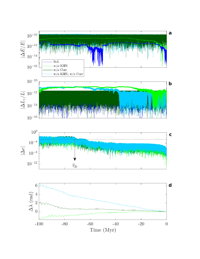
Figure 1: Solar system integrations over the past 100 Myr with orbitN. The standard setup (Std.) includes the planets, Pluto, ten asteroids, $J_{2}$, a lunar contribution, and 1PN corrections implemented following Saha & Tremaine (1994). KHN = Kahan compensated summation (Kahan, 1965). Corr = symplectic corrector (stage 6 = 7th order, see Wisdom, 2006). The timestep is $\Delta t=2$ days. $\Delta E/E=(E-E_{0})/E_{0}$ and $\Delta L_{z}/L$ indicate relative changes in energy and angular momentum. Differences in orbital eccentricity ($\Delta e$) and mean longitude ($\Delta\lambda$) are for the Earth-Moon barycenter, relative to the standard run. $\widehat{\tau}_{D}$ is the divergence time (see text).

For the present standard solar system integrations, initial conditions for the positions and velocities of the planets and Pluto were generated from the JPL DE431 ephemeris (Folkner et al., 2014) (naif.jpl.nasa.gov/pub/naif/generic_kernels/spk/planets), using the SPICE toolkit for Matlab (naif.jpl.nasa.gov/naif/toolkit.html). We have recently also tested the latest JPL ephemeris DE441 (Park et al., 2021), which makes little difference for practical applications because the divergence time relative to the astronomical solution ZB18a (based on DE431) is $\sim$66 Ma (see Section 4.2) and hence beyond ZB18a’s reliability limit of $\sim$58 Ma (based on geologic data, see below). The standard integration includes 10 asteroids, with initial conditions generated at ssd.jpl.nasa.gov/x/spk.html (for a list of asteroids, see Zeebe (2017)). Coordinates were obtained at JD2451545.0 in the ECLIPJ2000 reference frame and subsequently rotated to account for the solar quadrupole moment ($J_{2}$) alignment with the solar rotation axis (Zeebe, 2017). Our astronomical solutions are provided over the time interval from 100-0 Ma. However, as only the interval 58-0 Ma is constrained by geologic data (Zeebe & Lourens, 2019), we caution that the interval prior to 58 Ma is unconstrained due to solar system chaos. The standard integration includes the solar quadrupole moment $J_{2}=1.305\mbox{$\times 10^{-7}$}$, the lunar contribution, and 1PN corrections. Unless stated otherwise, the integration timestep is $\Delta t=2$ days, as previously used in our astronomical solution ZB18a (see Section 4.2), which also properly resolves Mercury’s pericenter (at eccentricity $\lesssim 0.2$), hence avoiding numerical chaos (see Wisdom, 2015; Hernandez et al., 2022).

As a first test, the long-term behavior of changes in energy ($\Delta E/E=(E-E_{0})/E_{0}$), angular momentum ($\Delta L_{z}/L$), and the implementation of Kahan compensated summation and symplectic correctors in orbitN is examined (Fig. 1). As should be expected from a symplectic algorithm, $|\Delta E/E|$ remains small ($|\Delta L_{z}/L|$ as well) and do not exhibit any significant trends over 100 Myr. Omitting Kahan summation, maximum $|\Delta E/E|$ and $|\Delta L_{z}/L|$ increase by up to a factor of $\sim$10. Omitting the symplectic corrector (stage 6 = 7th order, see Wisdom, 2006), the energy fluctuations that are removed by the corrector become apparent; the corrector has little effect on $|\Delta L_{z}/L|$. Omitting both Kahan summation and the corrector yields similar results to omitting just the corrector. The consequences for the dynamics of the system may be illustrated by examining the differences in the EMB’s orbital eccentricity ($\Delta e$) and mean longitude ($\Delta\lambda$), relative to the standard run (Fig. 1c and d). The effects of Kahan summation and the corrector on $\Delta e$ are similar to those of a small perturbation or a small difference in initial conditions, which grows over time (see below and Zeebe, 2015a, b, 2017). Notably, for practical applications in astrochronology over, say, the past 60 Myr or so, Kahan summation and symplectic correctors would actually make little difference because the divergence time to the standard solution is $\gtrsim$ 70 Ma (Fig. 1c), i.e., significantly beyond its reliability limit of $\sim$58 Ma (see above).

4.2 Astronomical solution ZB18a

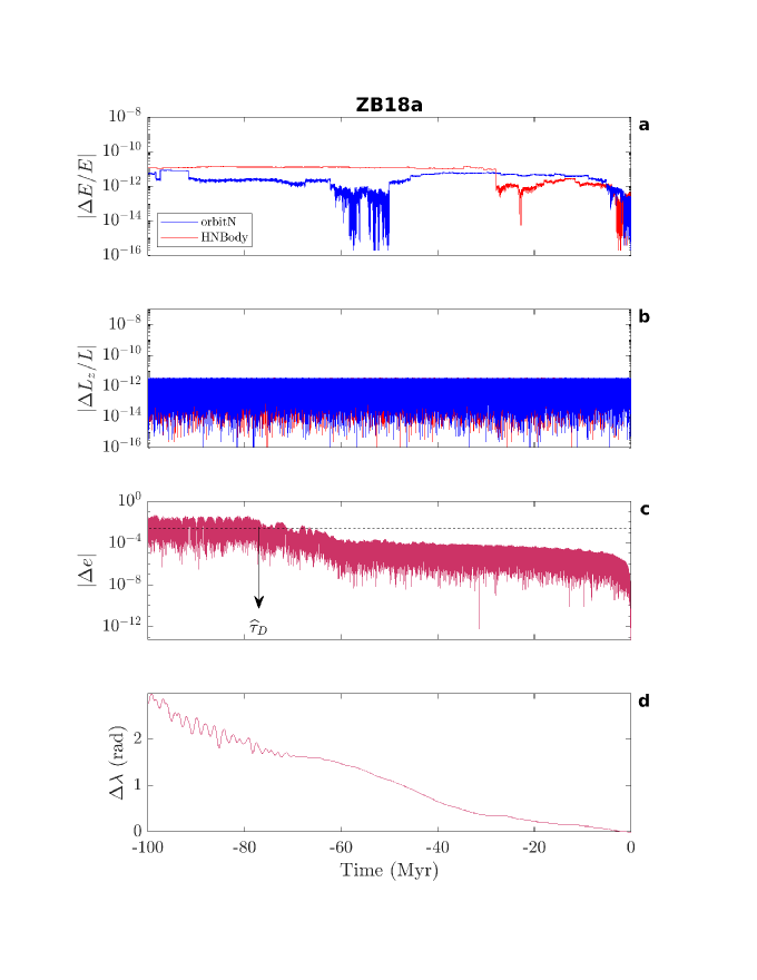
Figure 2: Comparison of solar system integrations with orbitN and HNBody for the setup of the astronomical solution ZB18a (Zeebe & Lourens, 2019, see text for details). $\Delta E/E=(E-E_{0})/E_{0}$ and $\Delta L_{z}/L$ indicate relative changes in energy and angular momentum. Differences in orbital eccentricity ($\Delta e$) and mean longitude ($\Delta\lambda$) are for the Earth-Moon barycenter. $\widehat{\tau}_{D}$ is the divergence time (see text).

The astronomical solution ZB18a was originally obtained with the integrator package HNBody (Rauch & Hamilton, 2002) (v1.0.10) using the same setup as described above and the symplectic integrator (2nd order WH map) with Jacobi coordinates (Zeebe & Lourens, 2019, 2022b). Earth’s orbital eccentricity for the ZB18a solution is available at www2.hawaii.edu/~zeebe/Astro.html and www.ncdc.noaa.gov/paleo/study/35174. In order to lend confidence to the accuracy and reproducibility of long-term orbital solutions for the solar system, it is imperative to compare the new standard solution obtained with orbitN (Section 4.1) to the original solution ZB18a (Fig. 2). The changes in $|\Delta E/E|$ and $|\Delta L_{z}/L|$ across the 100 Myr integration with orbitN and HNBody remain below $\mbox{$\sim$}1\mbox{$\times 10^{-11}$}$ and $\mbox{$\sim$}3\mbox{$\times 10^{-12}$}$ throughout the integrations.

The divergence time $\widehat{\tau}_{D}$ for Earth’s orbital eccentricity is $\sim$77 Ma (Fig. 2c), again far beyond the reliability limit of $\sim$58 Ma. $\widehat{\tau}_{D}\simeq 77$ Ma even exceeds the $\sim$72 Ma calculated for in- and excluding Kahan summation and symplectic correctors in a single integrator (orbitN, Fig. 1), suggesting that within the limits of the current physical model of the solar system, the performance of the integrators orbitN and HNBody is very similar.

4.3 Implementation of general relativity

As mentioned above, orbitN includes post-Newtonian corrections from general relativity due to $M_{0}$ (to 1PN order), implemented following ST94 (see Section 3.7), which also applies to HNBody. However, other methods of implementing 1PN corrections are possible. For example, the integrator package REBOUNDx provides 1PN-implementation options such as “gr_potential” (Nobili & Roxburgh, 1986) and “gr”, based on a 1st-order splitting (Tamayo et al., 2020). The option gr_potential represents a simplified $1/r^{2}$ perturbing potential, supposed to mimic the secular advance of perihelia from GR, as proposed by Nobili & Roxburgh (1986), who considered one out of three GR terms and ignored the other two GR terms that are small for the outer planets. The $1/r^{2}$ potential is known to incorrectly predict, for instance, the instantaneous elements. The option gr is more accurate but computationally expensive (see below). It turned out that ST94’s method is either more accurate or significantly faster than the REBOUNDx GR options. This is not a criticism of the REBOUNDx package, or the WH map as implemented in the REBOUND package (Rein & Tamayo, 2015). Indeed, both packages and their source code availability is very useful, including for developing and testing orbitN-1.0. The 1st-order split 1PN-implemententation in REBOUNDx had a specific intention (for details, see Tamayo et al., 2020) and is likely appropriate for many applications. However, when gr is combined with the WH map, for instance, auxiliary computations are required to integrate across the GR step, which results in a significant performance hit. For the user with a specific problem at hand, it seems important to be aware of the differences between various options available in different integrator packages and their characteristics, which may otherwise take a significant effort to figure out.

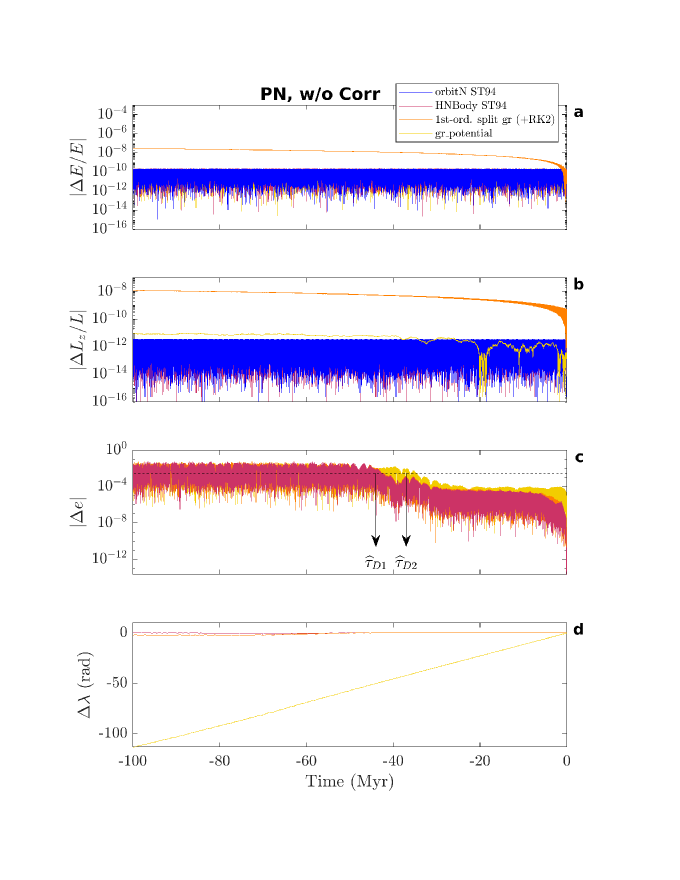
Figure 3: Comparison of solar system integrations with orbitN, HNBody, and REBOUND and different 1PN implementations (see text). The standard setup (Section 4.1) is used, except that in all packages, $J_{2}$, the lunar contribution (where available), and symplectic correctors are turned off. $\Delta E/E=(E-E_{0})/E_{0}$ and $\Delta L_{z}/L$ indicate relative changes in energy and angular momentum. Differences in orbital eccentricity ($\Delta e$) and mean longitude ($\Delta\lambda$) are for the Earth-Moon barycenter. $\widehat{\tau}_{D}$’s are divergence times (see text).

Regarding performance, it is noteworthy that the 1PN option (ST94) in orbitN and HNBody adds less than $\sim$10% computational overhead for the current application, while the gr_potential and gr (+RK2) options add $\sim$4% and $\sim$190% overhead, respectively. Overall, for the 1PN runs displayed in Fig. 3, orbitN was faster than the gr (+RK2) option by a factor of $\sim$2.6. Furthermore, orbitN was about as fast (Intel i9-12900 @2.40GHz) or $\sim$15% faster (Intel i5-10600 @3.30GHz) than HNBody v1.0.10, hence depending on hardware. All tests were performed on 64-bit Linux machines and gcc optimization level 3 for orbitN and REBOUND.

To facilitate a basic comparison, the standard solar system integration setup (Section 4.1) with a few modifications was run in orbitN, HNBody, and REBOUNDx (Fig. 3). In all packages, 1PN corrections were turned on, while $J_{2}$, the lunar contribution (where available), and symplectic correctors were turned off. In orbitN, the 1PN energy contribution was calculated according to Eq. (22), while in REBOUNDx, the functions rebx_gr_potential_potential() and rebx_gr_hamiltonian() were used. In orbitN, the 1PN angular momentum was calculated following Poisson & Will (2014), while in REBOUNDx no equivalent function seems available. In HNBody, routines for 1PN energy and angular momentum have apparently been coded (likely similar to those in orbitN, as can be inferred from the output) but the details are unavailable because the source code is inaccessible.

The results for $|\Delta E/E|$ and $|\Delta L_{z}/L|$ computed with orbitN and HNBody (both follow ST94’s 1PN implementation) are virtually identical, while $|\Delta E/E|$ and $|\Delta L_{z}/L|$ (for $t\lesssim-5$ Myr) increase linearly for the gr option (see Fig. 3, note logarithmic ordinate). The differences in the 1PN implementations also affect the orbital dynamics, showing significant differences in the EMB’s orbital eccentricity and mean longitude for gr_potential, while the gr results are closer to those of orbitN (Fig. 3c and d). The divergence time $\widehat{\tau}_{D}{}_{1}\simeq 44$ Myr for the difference in the EMB’s orbital eccentricity ($\Delta e$) between orbitN and HNBody (Fig. 3c) is typical for runs with 1PN corrections enabled but $J_{2}$ and the lunar contribution disabled (see Section 4.4). However, the corresponding $\widehat{\tau}_{D}{}_{2}\simeq 37$ Myr between orbitN and gr_potential is distinctly shorter. Thus, it appears that the numerical 1PN implementation can enhance the apparent chaos in the system.

Then how can one distinguish between numerical and physical effects on the system’s dynamics and apparent chaoticity? In other words, how can one tell whether one solution is more accurate than another? In the present case, the known limitations of gr_potential suggest that ST94’s method is more accurate, as illustrated by differences in the EMB’s orbital eccentricity and mean longitude (see Fig. 3c and d). Yet, $|\Delta E/E|$ and $|\Delta L_{z}/L|$ do not hint at problems with the gr_potential method, as long as $|\Delta E/E|$ is calculated within the framework of the $1/r^{2}$ perturbing potential (see Fig. 3a and b). Conversely, $|\Delta E/E|$ and $|\Delta L_{z}/L|$ for the gr option may raise a red flag, yet the calculated EMB’s orbital eccentricity and mean longitude are closer to ST94’s method. Testing divergence times of integrators for the same perturbation can also provide some insight to distinguish between methods (see Section 4.4). Further indications may be obtained by applying a different integrator algorithm to the same problem. For example, Zeebe (2017) showed that solar system integrations with HNBody but fundamentally different algorithms (non-symplectic Bulirsch-Stoer method vs. the symplectic WH map, both 1PN enabled) virtually agree to $\sim$63 Myr in the past, although this observation says more about the basic algorithms than the 1PN implementation. Thus, in summary, inspection of $|\Delta E/E|$ and $|\Delta L_{z}/L|$, as well as prior knowledge and additional tests can assist in finding suitable criteria to distinguish between numerical and physical effects on the system’s apparent chaoticity. However, identifying such criteria is not straightforward in the present case and can be even trickier in other cases.

4.4 $J_{2}$-, lunar-, and PN-Effects on Chaos

In the following, I use orbitN to provide insight into the effect of various physical processes on the long-term chaos in the solar system, including general relativity (PN), $J_{2}$ (J2), and the lunar contribution (LUN). For the standard setup ZB18a (see Section 4.2), the different physical effects were turned on and off in various combinations and for each combination, ensemble runs were performed ($K=16$), with Earth’s initial $x$-coordinate perturbed by $\Delta x^{k}_{0}=k\times 10^{-12}$ au ($k=0,\ldots,K-1$). Note that $\Delta x_{0}=10^{-12}$ au is much smaller than the difference in $x_{0}$, say, between different ephemerides such as DE431 and INPOP13c ($\Delta x_{0}\simeq 10^{-9}$ au, Zeebe, 2017). Next, $\widehat{\tau}_{D}$ was determined for each ensemble member relative to the respective reference run ($k=0$). The purpose of the above procedure is to examine the evolution of a small perturbation under the solar system’s chaotic dynamics and measure the exponential divergence of trajectories (using $\widehat{\tau}_{D}$) for different physical effects. Tendentially, the smaller $\widehat{\tau}_{D}$, the stronger the chaos. The ensembles provide some insight into the system’s multitude of solutions for a set of initial conditions and allow identifying exceptional runs (see below).

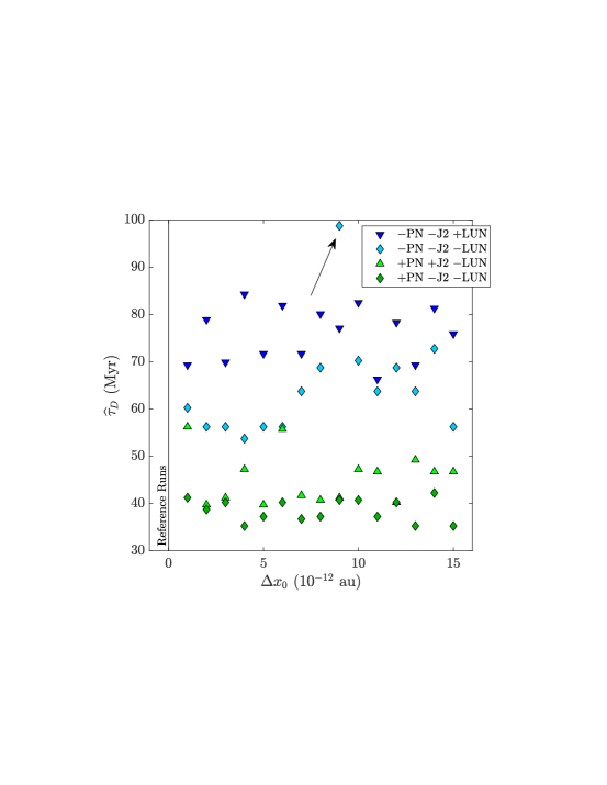
Figure 4: Ensemble integrations with orbitN turning on/off ($+/-$) general relativity (PN), $J_{2}$ (J2), and the lunar contribution (LUN) in different combinations. Earth’s initial $x$-coordinate is perturbed by $\Delta x_{0}$, relative to the corresponding reference run ($\Delta x_{0}=0$ au). $\widehat{\tau}_{D}$ is the divergence time (see text).

Turning on only PN gives the smallest $\widehat{\tau}_{D}$ of about 40 Myr ($+$PN $-$J2 $-$LUN, green diamonds, Fig. 4). Adding J2 stabilizes somewhat (green triangles), yet removing PN has an even more stabilizing effect (blue diamonds), increasing $\widehat{\tau}_{D}$ to $\sim$60-70 Myr ($-$PN $-$J2 $-$LUN, Fig. 4). Note that the run with $\widehat{\tau}_{D}\simeq 100$ Myr ($k=9$, blue diamond, arrow) is not an error or “outlier” that can therefore be excluded (the run was carefully examined). The run is a proper solution of the system, illustrating the inherent unpredictability of chaotic systems and their unaccountability in terms of conventional statistics. The effect of adding the lunar contribution ($-$PN $-$J2 $+$LUN, blue triangles, Fig. 4) increases $\widehat{\tau}_{D}$ from 60-70 to $\gtrsim$ 70 Myr. The possible causes behind these effects, as well as the different PN implementations (Section 4.3) in relation to the chaos in the system are discussed below considering the system’s fundamental frequencies (Section 4.5).

4.5 Changes in fundamental frequencies

Several resonances and their overlap have been proposed and investigated as the cause of the chaos in the solar system, including the $2(g_{4}-g_{3})-(s_{4}-s_{3})$ resonance and the interaction between $g_{5}$ (largely Jupiter’s forcing frequency) and $g_{1}$ as part of the $(g_{1}-g_{5})-(s_{1}-s_{2})$ resonance (Laskar, 1990; Sussman & Wisdom, 1992; Morbidelli, 2002; Ito & Tanikawa, 2002; Lithwick & Wu, 2011; Batygin et al., 2015; Zeebe, 2017; Mogavero & Laskar, 2022; Zeebe, 2022; Brown & Rein, 2023). The $g$’s and $s$’s (aka fundamental, or secular frequencies, eigenmodes, etc.) are constant in quasiperiodic systems but vary over time in chaotic systems, although some combinations such as $(g_{2}-g_{5})$ are more stable than others (for discussion, see e.g., Spalding et al., 2018). It is critical to recall that there is no simple 1-to-1 relationship between planet and eigenmode, particularly for the inner planets. The system’s motion is a superposition of all eigenmodes, although some modes represent the single dominant term for some (mostly outer) planets. The $g_{1}$-$g_{5}$ interaction, “$(g_{1}-g_{5})$” for short, can force Mercury’s eccentricity to high values and plays a critical role in the long-term stability of the solar system on Gyr time scale (e.g., Laskar, 1990; Batygin & Laughlin, 2008; Lithwick & Wu, 2011; Zeebe, 2015a; Abbot et al., 2023; Brown & Rein, 2023). Importantly, $(g_{1}-g_{5})$ is affected by general relativity, as PN corrections move $g_{1}$ up (by $\sim$0.43 ^′′/y at present) and away from $g_{5}$ (for illustration, see Fig. 4 in Zeebe, 2015a), thus reducing the tendency for instability on Gyr time scale.

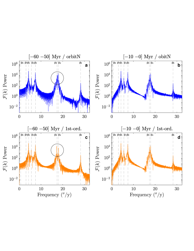
Figure 5: Time series analysis of Earth’s $k=e\cos(\varpi)$ (see text) across the intervals $-60$ to $-50$ Myr and $-10$ to $0$ Myr to extract solar system $g$-modes from runs with orbitN and REBOUND gr (+RK2) for different 1PN implementations (see Fig. 3). ${\cal F}=$ Fast-Fourier Transform (FFT). Vertical dashed lines indicate frequencies of $g$-modes (see Zeebe, 2017). Note differences in $g_{3}$ and $g_{4}$ in [$-60$ $-50$] Myr (circles in panels a and c).

On the contrary, PN corrections increase chaoticity (decrease the divergence time) in the current 100-Myr simulations (compare blue and green diamonds in Fig. 4), suggesting that other mechanisms, for example, the $2(g_{4}-g_{3})-(s_{4}-s_{3})$ resonance may be more important on 100-Myr time scale. Indeed, spectral analysis of, for instance, the present integrations comparing the 1st-order split and the symplectic 1PN implementation (cf. Fig. 3) reveal differences in $g_{3}$ and $g_{4}$ (see Fig. 5), as well as small differences in $s_{3}$ and $s_{4}$ (not shown), consistent with a recent analysis of variations in Earth’s and Mars’ orbital inclination and obliquity across the same time scale (Zeebe, 2022). Presuming that different resonances dominate on different time scales suggests a potential mechanism for GR corrections having opposite effects on Gyr- vs. 100-Myr time scale, say, through $(g_{1}-g_{5})$ vs. $(g_{4}-g_{3})$. As mentioned above, GR moves up $g_{1}$ and away from $g_{5}$ (the shift is much larger for $g_{1}$ than for $g_{5}$ and $g_{1}>g_{5}$). GR also moves up $g_{3}$ and $g_{4}$, and the shift is also (somewhat) larger for $g_{3}$ than for $g_{4}$ — however, in this case $g_{3}<g_{4}$. In this oversimplification, GR would hence increase $(g_{1}-g_{5})$ but decrease $(g_{4}-g_{3})$. While this notion appears consistent with the results of the integrations performed here (summarized in Fig. 4), spectral analysis of selected runs suggests a much more complex pattern, as detailed in the following. Below, spectra are presented based on the Fast-Fourier Transform (FFT), which was used to extract the fundamental frequencies ($g$’s and $s$’s) from the classic variables:

$$h=e\sin(\varpi)\quad \quad k=e\cos(\varpi)$$ ; (24)

$$p=\sin(I/2)\ \sin\Omega\quad \quad q=\sin(I/2)\ \cos\Omega\ ,$$ ; (25)

where $e$, $I$, $\varpi$, and $\Omega$ are eccentricity, inclination, longitude of perihelion, and longitude of ascending node, respectively.

For the two-body problem, the change in the argument of perihelion, $\omega$, due to GR may be written as (Einstein, 1916):

$$\dot{\omega}=24\pi^{3}\frac{a^{2}}{c^{2}T^{2}(1-e^{2})}\cdot T^{-1}\ ,$$ (26)

where $a$, $e$, and $T$ are the semimajor axis, eccentricity, and orbital period; $c$ is the speed of light and the factor $T^{-1}$ yields $\dot{\omega}$ per unit time (instead of per orbit). Eq. (26) gives $\dot{\omega}\simeq 0.43$, 0.038 and 0.014 ^′′/y for the orbits of Mercury, Earth, and Mars at present. Spectral analysis ($-$25 to 0 Myr) of runs with and without PN (blue/green diamonds, Fig. 4) give a shift of $\Delta g_{1}=0.36$ ^′′/y (Fig. 6a), indicating that $g_{1}$ reflects Mercury’s orbit but not in a simple manner, in which case one would expect $\Delta g_{1}=0.43$ ^′′/y. For the same runs, FFT yields $\Delta g_{3}=0.073$ ^′′/y and $\Delta g_{4}=0.055$ ^′′/y (Fig. 6a), showing large differences to Eq. (26) (which predicts $\dot{\omega}$ in a two-body system). Thus, while the FFT analysis shows similar tendencies to Eq. (26), the full interacting system is much more complex, as expected. As mentioned above, in general there is no simple 1-to-1 relationship between a single planet and a single eigenmode. Note also the large shift in $s_{2}$ (Fig. 6b).

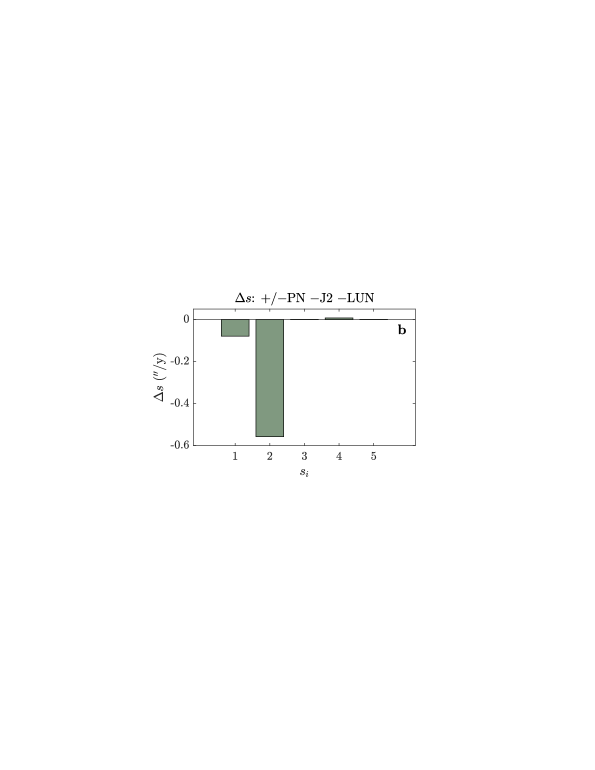
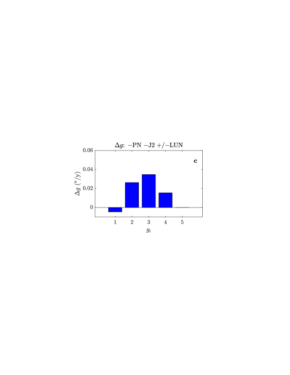
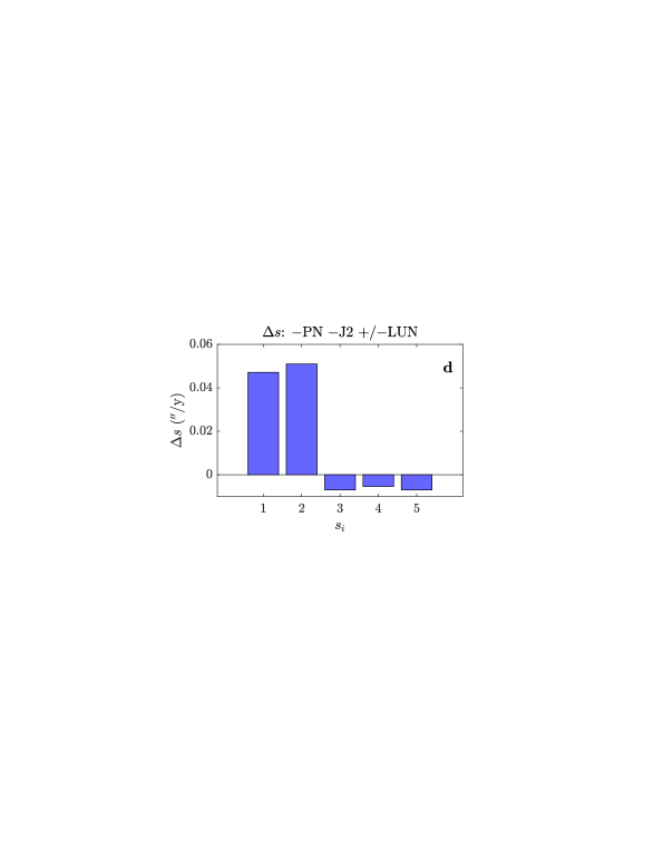
Figure 6: Shifts in fundamental frequencies ($\Delta g_{i}$ and $\Delta s_{i}$) from FFT analyses of runs shown in Fig. 4 ($\Delta x_{0}=10^{-12}$ au) across the interval $-$25 to 0 Myr. Shifts are calculated between two runs each with PN on/off $=+/-$ (green) and LUN on/off $=+/-$ (blue).

The stabilizing effect of the lunar contribution (compare blue diamonds and blue triangles in Fig. 4) appears similarly convoluted. The change in the argument of perihelion of the Earth-Moon barycenter due to the lunar contribution may be written as (see Eq. (21) and Appendix B):

$$\dot{\omega}=\frac{nB}{a^{2}(1-e^{2})^{2}}\ ;\ B = \frac{3\ m_{E}\ m_{L}\ R^{2}}{4\ (m_{E}+m_{L})^{2}}\cdot f_{L}\ ,$$ (27)

where $n$ is the mean motion. Eq. (27) gives $\dot{\omega}\simeq 0.066$ ^′′/y for the EMB’s orbit at present. Spectral analysis ($-$25 to 0 Myr) of runs with and without LUN give a smaller $g_{3}$ shift and, in addition, significant shifts in $g_{1}$, $g_{2}$, and $g_{4}$ (Fig. 6c), as well as sizable shifts in $s_{1}$ and $s_{2}$ (Fig. 6d). Note also that the results for $\Delta g_{i}$ and $\Delta s_{i}$ as presented in Fig. 6 depend on the time interval selected for spectral analysis. For example, across the interval $-$10 to 0 Myr, $\Delta g_{2}$ is actually larger than $\Delta g_{3}$ for the LUN on/off case. The numerical values of $2(g_{4}-g_{3})-(s_{4}-s_{3})$ and $(g_{1}-g_{5})-(s_{1}-s_{2})$ are close to zero for the runs analyzed. In summary, it is clear that while simplified views based on the two-body problem (e.g., Eqs. (26) and (27)) can be helpful as a starting point, they of course fail to capture the complexity of the long-term dynamics of the full system. Further in-depth analysis of the link between changes in fundamental frequencies, resonances, and chaos may require a detailed eigenmode analysis and signal reconstruction (e.g., Zeebe, 2017, 2022), which is beyond the goal of the current paper (that is, to introduce orbitN) and is hence left for future work.

5 Summary and Conclusions

I have introduced the symplectic integrator orbitN (version 1.0) with the primary goal of efficiently generating accurate and reproducible long-term orbital solutions for near-Keplerian planetary systems dominated by a central mass. orbitN-1.0 is suitable for hierarchical systems without close encounters but can be extended to include additional features in future versions. While the current orbitN application focuses on the solar system, orbitN can generally be applied to planetary systems with a dominant mass $M_{0}$. Among other features, orbitN-1.0 includes $M_{0}$’s quadrupole moment, a lunar contribution, and post-Newtonian corrections (1PN) due to $M_{0}$ based on a fast symplectic implementation. I have used orbitN to provide insight into the effect of various physical processes on the long-term chaos in the solar system. The integrations performed here reveal that 1PN corrections have the opposite effect on chaoticity/stability on 100-Myr time scale, as compared to Gyr-time scale. Finally, time series analysis was performed to examine the influence of different physical processes on fundamental frequencies, which affect secular resonances and, in turn, the long-term dynamics of the solar system.

Appendix A PN: $\alpha$-term

The term $\alpha_{j}\ {\cal H}^{2}_{Kep,j}$ in Eq. (23) leads to a scaling of the timestep argument of the Drift operator (Saha & Tremaine, 1994) as detailed in the following. Consider a single body first, i.e., drop index $j$ for the time being. Using Poisson brackets:

$$\{F,G\}=\frac{\partial F}{\partial\mbox{\boldmath$x$}}\frac{\partial G}{\partial\mbox{\boldmath$p$}}-\frac{\partial F}{\partial\mbox{\boldmath$p$}}\frac{\partial G}{\partial\mbox{\boldmath$x$}}\ ,$$ (A1)

Hamilton’s equations can be written as: ($\mbox{\boldmath$z$}=[\mbox{\boldmath$x$}\ \mbox{\boldmath$p$}]$):

$$\dot{\mbox{\boldmath$z$}}=\{\mbox{\boldmath$z$},{\cal H}\}\qquad\Rightarrow\qquad\dot{\mbox{\boldmath$x$}}=\frac{\partial{\cal H}}{\partial\mbox{\boldmath$p$}}\qquad;\qquad\dot{\mbox{\boldmath$p$}}=-\frac{\partial{\cal H}}{\partial\mbox{\boldmath$x$}}\ .$$ (A2)

If $\{\mbox{\boldmath$z$},{\cal H}\}\equiv{\cal D}$ is considered an operator acting on $z$, then:

$$\dot{\mbox{\boldmath$z$}}={\cal D}\ \mbox{\boldmath$z$}\ ,$$ (A3)

with the formal solution:

$$\mbox{\boldmath$z$}=\mbox{\boldmath$z$}_{0}\ e^{\tau{\cal D}}\ .$$ (A4)

Now let ${\cal H}={\cal H}_{Kep}+\alpha{\cal H}^{2}_{Kep}$ (only affecting the Drift operator), then

$$\dot{\mbox{\boldmath$z$}}\ = \ \{\mbox{\boldmath$z$},{\cal H}_{Kep}+\alpha{\cal H}^{2}_{Kep}\}$$ (A5)

$$\dot{\mbox{\boldmath$x$}}\ = \ \frac{\partial{\cal H}_{Kep}}{\partial\mbox{\boldmath$p$}}\ (1+2\alpha{\cal H}_{Kep})$$ (A6)

$$\dot{\mbox{\boldmath$p$}}\ = \ -\frac{\partial{\cal H}_{Kep}}{\partial\mbox{\boldmath$q$}}\ (1+2\alpha{\cal H}_{Kep})\ .$$ (A7)

${\cal H}_{Kep}$ yields the 2-body energy $-\mu m^{\prime}/2a$, where $a$ is the semimajor axis. Using $\alpha=3/(2m^{\prime}c^{2})$, it follows $2\alpha{\cal H}_{Kep}=-3\mu/(2c^{2}a)$. Finally, we can write:

$$\mbox{\boldmath$z$}=\mbox{\boldmath$z_{0}$}\ e^{\tau{\cal D}\ (1+2\alpha{\cal H})}=\mbox{\boldmath$z_{0}$}\ e^{\tau^{\prime}{\cal D}}\ ,$$ (A8)

with $\tau^{\prime}=\tau\ [1-3\mu/(2c^{2}a)]$. Comparing Eqs. (A4) and (A8) shows that inclusion of the $\alpha$-term only changes the timestep argument of the Drift operator. Reintroducing the body index $j$, it follows $\tau^{\prime}_{j}=[1-3\mu_{j}/(2c^{2}a_{j})]$, i.e., $\tau$ is scaled for each body individually, depending on mass factor $\mu_{j}$ and semimajor axis $a_{j}$.

Appendix B Lunar effect on $\dot{\omega}$ of EMB’s orbit

The quadrupole acceleration term due to the lunar contribution may be written as (Eq. (21)):

$$\mbox{\boldmath$a$}_{Q} = -\mu_{0}B\frac{\mbox{\boldmath$r$}}{r^{5}}\ ,$$ (B1)

where $\mu_{0}=G\mbox{$M_{0}$}$ and

$$B = \frac{3\ m_{E}\ m_{L}\ R^{2}}{4\ (m_{E}+m_{L})^{2}}\cdot f_{L}\ ,$$ (B2)

which can be derived from a potential ($\mbox{\boldmath$a$}_{Q}=-\nabla\Phi_{Q}$):

$$\Phi_{Q} = -\mu_{0}B\frac{1}{3r^{3}}\ .$$ (B3)

Upon averaging, $r^{3}$ may be replaced by $a^{3}(1-e^{2})^{3/2}$. Hence taking as the disturbing function:

$$\Re = \frac{\mu_{0}B}{3a^{3}(1-e^{2})^{3/2}}\ ,$$ (B4)

$\dot{\omega}$ is given by (Danby, 1988; Murray & Dermott, 1999):

$$\dot{\omega}=\frac{na\sqrt{1-e^{2}}}{\mu_{0}e}\frac{\partial\Re}{\partial e}\ ,$$ (B5)

where $n$ is the mean motion and $\partial\Re/\partial i=0$ was used ($i=$ inclination). Finally,

$$\dot{\omega}=\frac{nB}{a^{2}(1-e^{2})^{2}}\ .$$ (B6)

References

- Abbot et al. (2023) Abbot, D. S., Hernandez, D. M., Hadden, S., et al. 2023, Astrophys. J., 944, 190, doi: 10.3847/1538-4357/acb6ff
- Batygin & Laughlin (2008) Batygin, K., & Laughlin, G. 2008, Astrophys. J., 683, 1207, doi: 10.1086/589232
- Batygin et al. (2015) Batygin, K., Morbidelli, A., & Holman, M. J. 2015, Astrophys. J., 799, 120, doi: 10.1088/0004-637X/799/2/120
- Brown & Rein (2023) Brown, G., & Rein, H. 2023, MNRAS, doi: 10.1093/mnras/stad719
- Chambers (1999) Chambers, J. E. 1999, Mon. Not. R. Astron. Soc., 304, 793, doi: 10.1046/j.1365-8711.1999.02379.x
- Danby (1987) Danby, J. M. A. 1987, Celest. Mech., 40, 303, doi: 10.1007/BF01235847
- Danby (1988) —. 1988, Fundamentals of celestial mechanics (Willmann-Bell Inc., Richmond, VA)
- Duncan et al. (1998) Duncan, M. J., Levison, H. F., & Lee, M. H. 1998, Astron. J., 116, 2067, doi: 10.1086/300541
- Einstein (1916) Einstein, A. 1916, Annalen der Physik, VI. Folge, 49(7), 769, doi: 10.1002/andp.19163540702
- Folkner et al. (2014) Folkner, W. M., Williams, J. G., Boggs, D. H., Park, R. S., & Kuchynka, P. 2014, Interplanetary Network Progress Report, 196, 1
- Fukushima (1997) Fukushima, T. 1997, Celest. Mech. Dyn. Astron., 66, 309
- Hernandez & Dehnen (2017) Hernandez, D. M., & Dehnen, W. 2017, MNRAS, 468, 2614, doi: 10.1093/mnras/stx547
- Hernandez et al. (2022) Hernandez, D. M., Zeebe, R. E., & Hadden, S. 2022, MNRAS, 510, 4302, doi: 10.1093/mnras/stab3664
- IEEE (2019) IEEE. 2019, IEEE Std 754-2019, 1, doi: 10.1109/IEEESTD.2019.8766229
- Ito & Kojima (2005) Ito, T., & Kojima, S. 2005, Publ. Natl. Astro. Obs. Japan, 8, 17
- Ito & Tanikawa (2002) Ito, T., & Tanikawa, K. 2002, MNRAS, 336, 483, doi: 10.1046/j.1365-8711.2002.05765.x
- Kahan (1965) Kahan, W. 1965, Communications of the ACM, 8, 40
- Kaufmann (2005) Kaufmann, D. E. 2005, Swifter – an improved solar system integration software package, www.boulder.swri.edu/swifter
- Landau & Lifshitz (1971) Landau, L., & Lifshitz, E. 1971, The classical theory of fields (Pergamon Press, Oxford)
- Laskar (1990) Laskar, J. 1990, Icarus, 88, 266, doi: 10.1016/0019-1035(90)90084-M
- Laskar et al. (2011) Laskar, J., Fienga, A., Gastineau, M., & Manche, H. 2011, Astron. Astrophys., 532, A89, doi: 10.1051/0004-6361/201116836
- Levison & Duncan (1994) Levison, H. F., & Duncan, M. J. 1994, Icarus, 108, 18, doi: 10.1006/icar.1994.1039
- Lithwick & Wu (2011) Lithwick, Y., & Wu, Y. 2011, Astrophys. J., 739, 17 pp., doi: 10.1088/0004-637X/739/1/31
- Mikkola (1997) Mikkola, S. 1997, Celest. Mech. Dyn. Astron., 67, 145, doi: 10.1023/A:1008217427749
- Mikkola & Aarseth (1998) Mikkola, S., & Aarseth, S. J. 1998, New Astron., 3, 309, doi: 10.1016/S1384-1076(98)00018-9
- Mikkola & Innanen (1999) Mikkola, S., & Innanen, K. 1999, Celest. Mech. Dyn. Astr., 74, 59, doi: 10.1023/A:1008312912468
- Mogavero & Laskar (2022) Mogavero, F., & Laskar, J. 2022, Astron. Astrophys., 662, L3, doi: 10.1051/0004-6361/202243327
- Morbidelli (2002) Morbidelli, A. 2002, Modern Celestial Mechanics: Aspects of Solar System Dynamics (Taylor & Francis, London)
- Murray & Dermott (1999) Murray, C. D., & Dermott, S. F. 1999, Solar system dynamics (Cambridge, UK: Cambridge University Press, pp. 592)
- Nobili & Roxburgh (1986) Nobili, A., & Roxburgh, I. W. 1986, in Relativity in Celestial Mechanics and Astrometry. High Precision Dynamical Theories and Observational Verifications, ed. J. Kovalevsky & V. A. Brumberg, Vol. 114, 105
- Park et al. (2021) Park, R. S., Folkner, W. M., Williams, J. G., & Boggs, D. H. 2021, Astron. J., 161, 105, doi: 10.3847/1538-3881/abd414
- Poisson & Will (2014) Poisson, E., & Will, C. M. 2014, Gravity: Newtonian, Post-Newtonian, Relativistic (Cambridge, pp. 780: Cambridge University Press)
- Quinn et al. (1991) Quinn, T. R., Tremaine, S., & Duncan, M. 1991, Astron. J., 101, 2287, doi: 10.1086/115850
- Rauch & Hamilton (2002) Rauch, K. P., & Hamilton, D. P. 2002, in Bull. Am. Astron. Soc., Vol. 34, AAS/Division of Dynamical Astronomy Meeting #33, 938
- Rauch & Holman (1999) Rauch, K. P., & Holman, M. 1999, Astron. J., 117, 1087, doi: 10.1086/300720
- Rein & Liu (2012) Rein, H., & Liu, S. F. 2012, Astron. Astrophys., 537, A128, doi: 10.1051/0004-6361/201118085
- Rein & Tamayo (2015) Rein, H., & Tamayo, D. 2015, MNRAS, 452, 376, doi: 10.1093/mnras/stv1257
- Saha & Tremaine (1994) Saha, P., & Tremaine, S. 1994, Astron. J., 108, 1962, doi: 10.1086/117210
- Spalding et al. (2018) Spalding, C., Fischer, W. W., & Laughlin, G. 2018, ApJ, 869, L19, doi: 10.3847/2041-8213/aaf219
- Stiefel & Scheifele (1975) Stiefel, E. L., & Scheifele, G. 1975, Linear and regular celestial mechanics (Springer-Verlag, Berlin)
- Stumpff (1959) Stumpff, K. 1959, Himmelsmechanik. Bd. 1: Das Zweikörperproblem und die Methoden der Bahnbestimmung der Planeten und Kometen (Deutscher Verlag der Wissenschaften, Berlin)
- Sussman & Wisdom (1992) Sussman, G. J., & Wisdom, J. 1992, Science, 257, 56, doi: 10.1126/science.257.5066.56
- Tamayo et al. (2020) Tamayo, D., Rein, H., Shi, P., & Hernandez, D. M. 2020, MNRAS, 491, 2885, doi: 10.1093/mnras/stz2870
- Varadi et al. (2003) Varadi, F., Runnegar, B., & Ghil, M. 2003, Astrophys. J., 592, 620, doi: 10.1086/375560
- Will (2014) Will, C. M. 2014, Phys. Rev. D, 89, 044043, doi: 10.1103/PhysRevD.89.044043
- Wisdom (2006) Wisdom, J. 2006, Astron. J., 131, 2294, doi: 10.1086/500829
- Wisdom (2015) —. 2015, Astron. J., 150, 127, doi: 10.1088/0004-6256/150/4/127
- Wisdom (2018) —. 2018, MNRAS, 474, 3273, doi: 10.1093/mnras/stx2906
- Wisdom & Holman (1991) Wisdom, J., & Holman, M. 1991, Astron. J., 102, 1528, doi: 10.1086/115978
- Wisdom & Holman (1992) —. 1992, Astron. J., 104, 2022, doi: 10.1086/116378
- Yoshida (1990) Yoshida, H. 1990, Physics Letters A, 150, 262, doi: 10.1016/0375-9601(90)90092-3
- Zeebe (2015a) Zeebe, R. E. 2015a, Astrophys. J., 798, 8, doi: 10.1088/0004-637X/798/1/8
- Zeebe (2015b) Zeebe, R. E. 2015b, Astrophys. J., 811, 9, doi: 10.1088/0004-637X/811/1/9
- Zeebe (2017) Zeebe, R. E. 2017, Astron. J., 154, 193, doi: 10.3847/1538-3881/aa8cce
- Zeebe (2022) —. 2022, Astron. J., 164, 107, doi: 10.3847/1538-3881/ac80f8
- Zeebe & Lourens (2019) Zeebe, R. E., & Lourens, L. J. 2019, Science, 365, 926
- Zeebe & Lourens (2022b) —. 2022b, Earth Planet. Sci. Lett., 592, 117595, doi: 10.1016/j.epsl.2022.117595