Abstract

Several hints of the presence of a new state at about $95$ GeV have been observed recently. The CMS and ATLAS collaborations have reported excesses in the diphoton channel at about this diphoton invariant mass with local statistical significances of $2.9\,\sigma$ and $1.7\,\sigma$, respectively. Furthermore, a $2\,\sigma$ excess in the $b\bar{b}$ final state was also observed at LEP, again pointing at a similar mass value. We interpret these intriguing hints of new physics in a variant of the Scotogenic model, an economical scenario that induces Majorana neutrino masses at the loop level and includes a viable dark matter candidate. We show that our model can naturally explain the 95 GeV excesses while respecting all experimental constraints and discuss other phenomenological predictions of our scenario.

1 Introduction

The Standard Model (SM) of particle physics has been an incredibly successful framework for understanding the fundamental particles and forces that make up our Universe. However, it faces significant challenges when it comes to explaining two crucial phenomena: neutrino masses and dark matter (DM). Neutrinos were long thought to be massless, as suggested by the original formulation of the SM. However, experimental evidence has now firmly established that neutrinos do have masses, albeit very small ones. Similarly, the existence of DM, which is inferred from its gravitational effects on visible matter, poses another major challenge and various theoretical extensions of the SM have been proposed to account for it. Explaining the origins and properties of neutrino masses and DM continues to be an active area of research.

After the discovery of the Higgs boson, which proved the existence of a scalar field and provided important insights into the mechanism of mass generation, the LHC has continued to search for additional scalar particles. In fact, many Beyond the Standard Model (BSM) scenarios include new scalar states. This is also the case of models addressing the neutrino and DM problems, which typically require extended scalar sectors. If these new states have masses and couplings within the reach of the LHC, their signals may be hidden in the currently existing searches or show up in the near future, and may appear at lower or higher masses than the scalar found at the LHC at a mass of 125 GeV. If lighter states exist, they may be produced given the high energies available at colliders. In fact, different experiments have performed searches for low mass scalars in different channels [1, 2, 3, 4, 5, 6, 7, 8, 9, 10, 11].

The diphoton channel plays a crucial role in the search for new scalar particles at the LHC. This final state allows for precise measurements and clean experimental signatures, making it easier to isolate potential signals of new scalar particles amidst background noise. Interestingly, the CMS collaboration has been consistently finding an excess over the SM prediction in this channel at a diphoton invariant mass of $\sim 95$ GeV [5, 6]. The statistical support for this excess has been reinforced by recent results obtained after the analysis of the full Run 2 dataset [7]. The excess is maximal for a mass of $95.4$ GeV and has a local (global) significance of $2.9\,\sigma$ ($1.3\,\sigma$) and can be interpreted as the production via gluon fusion and subsequent decay of a new scalar state, $h_{95}$. It can be parametrized numerically in terms of the $\mu_{\gamma\gamma}$ signal strength, which normalizes the cross section of the process to the analogous cross section for a Higgs-like state $H$ at the same mass. The latest CMS result points to [7, 12]

$$\mu^{\rm CMS}_{\gamma\gamma}=\frac{\sigma^{\rm CMS}(gg\to h_{95}\to\gamma\gamma)}{\sigma^{\rm SM}(gg\to H\to\gamma\gamma)}=0.33^{+0.19}_{-0.12}\,.$$ (1)

The ATLAS collaboration has also performed searches in the diphoton channel, although with a lower sensitivity. A very mild excess in a mass region compatible with that hinted by CMS was found in their Run 1 analysis [8]. Their update including 140 fb^-1 of Run 2 data appeared recently [13]. Intriguingly, the statistical significance of the excess increases in the new ATLAS results. This can be attributed to the addition of more statistics as well as to several improvements in the analysis. In particular, the model-dependent analysis presented in this update hints at an excess, curiously at $95.4$ GeV too, with a local significance of $1.7\,\sigma$. We note that this result is compatible with that of CMS, which ATLAS cannot exclude.

The 95 GeV region is particularly interesting due to the existence of other excesses hinting at similar mass values. LEP has reported an excess in $b\bar{b}$ production at about 95 GeV with a local significance of $2\,\sigma$ [2]. This excess can be interpreted in terms of a new scalar state contributing to the process $e^{+}e^{-}\to Z\,h_{95}\to Z\,b\bar{b}$, with a signal strength given by [14, 15]

$$\mu^{\rm LEP}_{bb}=\frac{\sigma^{\rm LEP}(e^{+}e^{-}\to Z\,h_{95}\to Z\,b\bar{b})}{\sigma^{\rm SM}(e^{+}e^{-}\to Z\,H\to Z\,b\bar{b})}=0.117\pm 0.057\,.$$ (2)

Other searches for light scalars in CMS also gave a small excess in the ditau channel $\mu_{\tau\tau}^{\rm CMS}=1.2\pm 0.5$ [10]. ATLAS has not published any ditau search in this mass region, but has only provided results for scalar masses above $200$ GeV [16].

The 95 GeV excesses have received some attention recently [15, 17, 18, 19, 20, 21, 22, 23, 24, 25, 26, 27, 28, 29, 30, 31, 32, 33, 34, 35]. We interpret them in a variant of the Scotogenic model [36], a well-motivated and economical BSM scenario that incorporates a mechanism for the generation of neutrino masses and provides a testable DM candidate. We thus consider the possibility that these excesses are the first collider hints of a new BSM sector addressing some of the most important open questions in particle physics.

The rest of the manuscript is organized as follows. Section 2 introduces our model, whereas Section 3 interprets the 95 GeV excesses in terms of a new scalar state in the particle spectrum. The most relevant experimental constraints are discussed in Section 4 and our numerical results, which prove that our setup can accommodate the excesses, are presented in Section 5. Other aspects of our scenario, such as neutrino masses, DM and additional collider signatures, are discussed in Section 6. Finally, we summarize our work in Section 7. An Appendix is also included with some technical details.

2 The Model

We consider a variant of the Scotogenic model [36] that extends the SM particle content with $n_{N}$ generations of singlet fermions $N_{n}$, $n=1,\dots,n_{N}$, and $n_{\eta}$ doublet scalars $\eta_{a}$, $a=1,\dots,n_{\eta}$. These fields are assumed to be odd under a new $\mathbb{Z}_{2}$ symmetry, under which all the SM states are even. This generalizes the original Scotogenic model [37], which corresponds to $n_{N}=3$ and $n_{\eta}=1$. The $\eta_{a}$ doublets can be decomposed in terms of their $\rm SU(2)_{L}$ components as

$$\eta_{a}=\left(\begin{array}[]{c}\eta_{a}^{+}\\ \eta_{a}^{0}\end{array}\right)\,.$$ (3)

In addition, we include a real singlet scalar $S$. The lepton and scalar particle content of the model is summarized in Tab. 1.

Field	Generations	$\boldsymbol{\rm SU(3)_{c}}$	$\boldsymbol{\rm SU(2)_{L}}$	$\boldsymbol{\rm U(1)_{Y}}$	$\boldsymbol{\mathbb{Z}_{2}}$
$\ell_{L}$	$3$	1	2	-1/2	+
$e_{R}$	$3$	1	1	-1	+
$N$	$n_{N}$	1	1	0	-
$H$	$1$	1	2	1/2	+
$\eta$	$n_{\eta}$	1	2	1/2	-
$S$	$1$	1	1	0	+

Table 1: Lepton and scalar particle content of the model and their representations under gauge and global symmetries.

The Yukawa Lagrangian of the model includes the terms

$$\mathcal{L}\supset y_{na\alpha}\,\overline{N}_{n}\widetilde{\eta}_{a}^{\dagger}\ell_{L}^{\alpha}-\kappa_{nm}\,S\,\overline{N^{c}}_{n}N_{m}-\frac{1}{2}\left(M_{N}\right)_{nn}\overline{N^{c}}_{n}N_{n}+\text{h.c.}\,,$$ (4)

where $n,m=1,\dots,n_{N}$, $a=1,\dots,n_{\eta}$ and $\alpha=1,2,3$ are generation indices. The Yukawa coupling $y$ is an $n_{N}\times n_{\eta}\times 3$ object while $\kappa$ and $M_{N}$ are $n_{N}\times n_{N}$ symmetric matrices. $M_{N}$ has been chosen diagonal without loss of generality. Finally, we define $\widetilde{\eta}=i\sigma_{2}\eta^{*}$. The scalar potential of the model can be written as

$$\mathcal{V}=\mathcal{V}_{H}+\mathcal{V}_{\eta}+\mathcal{V}_{S}+\mathcal{V}_{\rm mix}\,,$$ (5)

with

$$\mathcal{V}_{H}= m_{H}^{2}\,H^{\dagger}H+\frac{1}{2}\lambda_{1}\,\left(H^{\dagger}H\right)^{2}\,,$$ (6)

$$\mathcal{V}_{\eta}= \left(m_{\eta}^{2}\right)_{aa}\eta_{a}^{\dagger}\eta_{a}+\frac{1}{2}\lambda_{2}^{abcd}\left(\eta_{a}^{\dagger}\eta_{b}\right)\left(\eta_{c}^{\dagger}\eta_{d}\right)\,,$$ (7)

$$\mathcal{V}_{S}= \frac{1}{2}m_{S}^{2}\,S^{2}+\frac{1}{3}\mu_{S}\,S^{3}+\frac{1}{4}\lambda_{S}\,S^{4}\,,$$ (8)

$$\mathcal{V}_{\rm mix}= \lambda_{3}^{ab}\left(H^{\dagger}H\right)\left(\eta_{a}^{\dagger}\eta_{b}\right)+\lambda_{4}^{ab}\left(H^{\dagger}\eta_{a}\right)\left(\eta_{b}^{\dagger}H\right)+\frac{1}{2}\left[\lambda_{5}^{ab}\left(H^{\dagger}\eta_{a}\right)\left(H^{\dagger}\eta_{b}\right)+\text{h.c.}\right]$$

$$+\mu_{H}\,H^{\dagger}HS+\frac{1}{2}\lambda_{HS}\,H^{\dagger}HS^{2}+\mu_{\eta}^{ab}\,\eta_{a}^{\dagger}\eta_{b}\,S+\frac{1}{2}\lambda_{\eta S}^{ab}\,\eta_{a}^{\dagger}\eta_{b}\,S^{2}\,.$$ (9)

Here all the indices are $\eta$ generation indices and then $m_{\eta}^{2}$, $\lambda_{3,4,5}$, $\mu_{\eta}$ and $\lambda_{\eta S}$ are $n_{\eta}\times n_{\eta}$ matrices, while $\lambda_{2}$ is an $n_{\eta}\times n_{\eta}\times n_{\eta}\times n_{\eta}$ object. We also note that $\lambda_{5}$ must be symmetric whereas $\lambda_{3,4}$, $\mu_{\eta}$ and $\lambda_{\eta S}$ are Hermitian. Again, $m_{\eta}^{2}$ will be assumed to be diagonal without any loss of generality.

2.1 Symmetry breaking, scalar masses and mixings

We will assume that the vacuum of our model is given by

$$\langle H^{0}\rangle=\frac{v}{\sqrt{2}}\,,\quad\langle\eta^{0}_{a}\rangle=0\,,\quad\langle S\rangle=v_{S}\,.$$ (10)

The vacuum expectation value (VEV) $v$ breaks the electroweak symmetry in the usual way. In contrast, the $\mathbb{Z}_{2}$ Scotogenic parity remains exactly conserved due to $\langle\eta_{a}^{0}\rangle=0$. The VEV configuration in Eq. (10) imposes some conditions on the scalar potential parameters due to the minimization equations

$$\left.\frac{\partial V}{\partial H}\right|_{\langle H\rangle=\frac{v}{\sqrt{2}}\,,\,\langle S\rangle=v_{S}}= m_{H}^{2}v+\mu_{H}v\,v_{S}+\frac{1}{2}\lambda_{1}v^{3}+\frac{1}{2}\lambda_{HS}v_{S}^{2}v=0\,,$$ (11)

$$\left.\frac{\partial V}{\partial S}\right|_{\langle H\rangle=\frac{v}{\sqrt{2}}\,,\,\langle S\rangle=v_{S}}= m_{S}^{2}v_{S}+\mu_{S}v_{S}^{2}+\frac{1}{2}\mu_{H}v^{2}+\lambda_{S}v_{S}^{3}+\frac{1}{2}\lambda_{HS}v^{2}\,v_{S}=0\,.$$ (12)

After symmetry breaking, the real component of the neutral $H^{0}$ field mixes with the real $S$ field. In the basis $\mathcal{H}=\left\{S,\text{Re}(H^{0})\right\}$ their mass matrix reads

$$\mathcal{M}_{\mathcal{H}}^{2}=\left(\begin{matrix}m_{S}^{2}+2\mu_{S}v_{S}+\frac{1}{2}\lambda_{HS}\,v^{2}+3\lambda_{S}v_{S}^{2}&\mu_{H}v+\lambda_{HS}\,v\,v_{S}\\ \mu_{H}v+\lambda_{HS}\,v\,v_{S}&m_{H}^{2}+\mu_{H}v_{S}+\frac{3}{2}\lambda_{1}v^{2}+\frac{1}{2}\lambda_{HS}\,v_{S}^{2}\end{matrix}\right)\,.$$ (13)

After application of Eqs. (11) and (12), solved for $m_{H}^{2}$ and $m_{S}^{2}$, this matrix becomes

$$\mathcal{M}_{\mathcal{H}}^{2}=\left(\begin{matrix}v_{S}\left(\mu_{S}+2\lambda_{S}v_{S}\right)-\frac{\mu_{H}v^{2}}{2v_{S}}&\mu_{H}v+\lambda_{HS}\,v\,v_{S}\\ \mu_{H}v+\lambda_{HS}\,v\,v_{S}&\lambda_{1}v^{2}\end{matrix}\right)\,.$$ (14)

It can be brought to diagonal form as $V_{\mathcal{H}}\,\mathcal{M}^{2}_{\mathcal{H}}\,V_{\mathcal{H}}^{T}=\widehat{\mathcal{M}}^{2}_{\mathcal{H}}=\text{diag}\left(m^{2}_{h_{1}},m^{2}_{h_{2}}\right)$, where $h_{1}$ and $h_{2}$ are mass eigenstates and

$$V_{\mathcal{H}}=\left(\begin{matrix}\cos\alpha&\sin\alpha\\ -\sin\alpha&\cos\alpha\end{matrix}\right)\,,$$ (15)

with

$$\tan 2\alpha=\frac{2\,\left(\mathcal{M}^{2}_{\mathcal{H}}\right)_{12}}{\left(\mathcal{M}^{2}_{\mathcal{H}}\right)_{11}-\left(\mathcal{M}^{2}_{\mathcal{H}}\right)_{22}}\,.$$ (16)

This mixing angle between the singlet and doublet scalars plays a central role in the phenomenology of our model, as we will explain in the following Subsection. We focus now on the $\mathbb{Z}_{2}$-odd scalars $\eta^{+}_{a}$ and $\eta^{0}_{a}$. We decompose the neutral components of the $\eta_{a}$ doublets as

$$\eta_{a}^{0}=\frac{1}{\sqrt{2}}(\eta_{R_{a}}+i\eta_{I_{a}})\,,$$ (17)

and they do not mix if we assume that CP is conserved in the scalar sector. This can be easily achieved if all the parameters in the scalar potential are real. Again, after electroweak symmetry breaking, the $n_{\eta}\times n_{\eta}$ mass matrices are given by

$$\bigl{(}\mathcal{M}_{\eta_{R}}^{2}\bigr{)}_{ab} =\left(m_{\eta}^{2}\right)_{ab}+\left(\lambda_{3}^{ab}+\lambda_{4}^{ab}+\lambda_{5}^{ab}\right)\frac{v^{2}}{2}+\frac{v_{S}^{2}}{2}\lambda_{\eta S}^{ab}+\mu_{\eta}^{ab}v_{S}\,,$$ (18)

$$\bigl{(}\mathcal{M}_{\eta_{I}}^{2}\bigr{)}_{ab} =\left(m_{\eta}^{2}\right)_{ab}+\left(\lambda_{3}^{ab}+\lambda_{4}^{ab}-\lambda_{5}^{ab}\right)\frac{v^{2}}{2}+\frac{v_{S}^{2}}{2}\lambda_{\eta S}^{ab}+\mu_{\eta}^{ab}v_{S}\,,$$ (19)

$$\bigl{(}\mathcal{M}_{\eta^{+}}^{2}\bigr{)}_{ab} =\left(m_{\eta}^{2}\right)_{ab}+\lambda_{3}^{ab}\frac{v^{2}}{2}+\frac{v_{S}^{2}}{2}\lambda_{\eta S}^{ab}+\mu_{\eta}^{ab}v_{S}\,.$$ (20)

Notice that the mass matrices for the real and imaginary components are the same in the limit in which all the elements of $\lambda_{5}$ vanish.

2.2 Scalar couplings

Figure 1: 1-loop contributions to $h_{i}\to\gamma\gamma$.

The couplings of the $h_{1}$ and $h_{2}$ scalars to the SM fermions are determined by the $\alpha$ mixing angle which, as discussed below, will be constrained to be small. We note that the singlet $S$ does not have a Yukawa term with the SM fermions. Hence, it can only couple to them via mixing with the SM Higgs $H$. As a result of this, one of the mass eigenstates ($h_{1}$, the mostly-singlet one) couples to the SM fermions proportional to $\sin\alpha$ while the other mass eigenstate ($h_{2}$, the SM-like one) couples proportional to $\cos\alpha$. The same happens for the coupling to $WW$ and $ZZ$ bosons and the loop coupling to gluons. However, the 1-loop couplings to $\gamma\gamma$ and $\gamma Z$ will be affected by the new particle content present in our model, in particular the $\eta$ doublets. In Fig. 1 we can see the different contributions to the loop decays $h_{i}\to\gamma\gamma$. Similar diagrams can be drawn for the $\gamma Z$ final state. On the one hand the Higgses will couple to $\gamma\gamma/Z$ through the SM loops with $W$ bosons and fermions, with the largest contribution among the fermions given by the top quark. On the other hand, the charged $\eta$ states can also run into the loop and contribute to the decay through the $g_{h_{i}\eta\eta}$ coupling, given by

$$g_{h_{i}\eta\eta}=\left(V_{\mathcal{H}}\right)_{i1}(\lambda_{\eta S}\,v_{S}+\mu_{\eta})+\left(V_{\mathcal{H}}\right)_{i2}\,\lambda_{3}\,v\,,$$ (21)

or, equivalently,

$$g_{h_{1}\eta\eta}= \cos\alpha\left(\lambda_{\eta S}\,v_{S}+\mu_{\eta}\right)+\sin\alpha\,\lambda_{3}\,v\,,$$ (22)

$$g_{h_{2}\eta\eta}= -\sin\alpha\left(\lambda_{\eta S}\,v_{S}+\mu_{\eta}\right)+\cos\alpha\,\lambda_{3}\,v\,.$$ (23)

2.3 Neutrino masses

After symmetry breaking, the $n_{N}\times n_{N}$ mass matrix of the singlet fermions is given by

$$\mathcal{M}_{N}=M_{N}+2\,\kappa\,v_{S}\,.$$ (24)

As already explained, one can take the matrix $M_{N}$ to be diagonal without loss of generality. We will further assume that $\kappa$ is diagonal too. Then, the singlet fermion masses are simply given by $m_{N_{n}}=\left(\mathcal{M}_{N}\right)_{nn}=\left(M_{N}\right)_{nn}+2\,\kappa_{nn}\,v_{S}$.

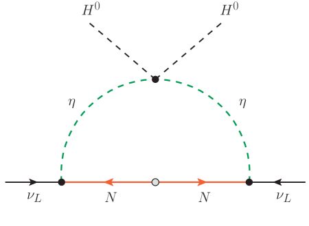
Figure 2: Neutrino mass generation in our model.

The simultaneous presence of the $y$ and $\lambda_{5}$ couplings and the $M_{N}$ Majorana mass term (or the $\kappa$ coupling) leads to explicit lepton number violation. Neutrino masses vanish at tree-level due to the $\mathbb{Z}_{2}$ symmetry of the model, that forbids a neutrino Yukawa interaction with the SM Higgs doublet. However, neutrinos acquire non-zero Majorana masses at the 1-loop, as shown in Fig. 2. This mechanism is exactly the same as in the original Scotogenic model [36], although our scenario includes a variable number of $N$ and $\eta$ fields. The general expression for the light neutrinos Majorana mass matrix can be found in [37] where it is particularized for specific $(n_{N},n_{\eta})$ cases.

3 Interpretation of the 95 GeV excesses

In the following we will assume that the lightest $\mathbb{Z}_{2}$-even scalar in our model, $h_{1}$, has a mass of 95 GeV and is thus identified with the scalar resonance hinted by CMS, ATLAS and LEP precisely this energy scale. Therefore, $h_{2}$ is identified with the 125 GeV Higgs discovered at the LHC. In summary,

$$h_{1}\equiv h_{95}\,,\quad h_{2}\equiv h_{125}\,.$$ (25)

We should then study whether our model can accommodate the experimental hints at 95 GeV. In other words, we must determine the regions in the parameter space leading to a $h_{1}$ diphoton signal strength in agreement with Eq. (1) that also comply with the existing experimental constraints. We will also explore the possibility to simultaneously explain the other anomalies at 95 GeV, in the $b\bar{b}$ and ditau channels.

The signal strength for the diphoton channel is given in our model by

$$\mu_{\gamma\gamma}=\frac{\sigma(gg\to h_{1})}{\sigma_{\rm SM}(gg\to H)}\times\frac{{\rm BR}(h_{1}\to\gamma\gamma)}{{\rm BR}_{\rm SM}(H\to\gamma\gamma)}=\sin^{2}\alpha\,\frac{{\rm BR}(h_{1}\to\gamma\gamma)}{{\rm BR}_{\rm SM}(H\to\gamma\gamma)}\,,$$ (26)

where we normalize again to the SM values, the usual suppression by the $\alpha$ mixing angle has been taken into account and ${\rm BR}(h_{1}\to\gamma\gamma)$ is the $h_{1}\to\gamma\gamma$ branching ratio in our model. This is modified with respect to the predicted value for a Higgs-like state with a mass of 95 GeV due to the presence of the $\eta$ doublets. The decay width of a CP-even scalar to two photons has been studied in great detail [38, 39, 40]. With $n_{\eta}$ generations of $\eta$ doublets and assuming diagonal $g_{h_{i}\eta\eta}$ couplings, it is given by

$$\Gamma(h_{i}\to\gamma\gamma)=\frac{G_{F}\alpha^{2}m_{h_{i}}^{3}}{128\sqrt{2}\pi^{3}}\left|\sum_{f}N_{c}Q_{f}^{2}g_{h_{i}ff}\,A_{1/2}(\tau_{f})+g_{h_{i}WW}\,A_{1}(\tau_{W})+\sum_{a}\frac{v}{2m^{2}_{\eta_{a}}}g_{h_{i}\eta\eta}^{aa}\,A_{0}(\tau_{\eta})\right|^{2}\,,$$ (27)

where $\tau_{k}=m^{2}_{h_{i}}/4m^{2}_{k}$ and the $A_{i}(\tau)$ functions are defined in Appendix A. As we can see, the presence of the $\eta$ doublets not only modifies the diphoton decay of the mostly-singlet state, but it also affects to the diphoton decay of the SM-like Higgs. As discussed below in Sec. 4, this feature constrains the parameter space from the existing measurements of the 125 GeV Higgs.

For the $b\bar{b}$ excess in LEP we must consider the signal strength

$$\mu_{bb}=\frac{\sigma(e^{+}e^{-}\to Z\,h_{1})}{\sigma_{\rm SM}(e^{+}e^{-}\to Z\,H)}\times\frac{{\rm BR}(h_{1}\to b\bar{b})}{{\rm BR}_{\rm SM}(H\to b\bar{b})}=\sin^{2}\alpha\,\frac{\Gamma(h_{1}\to b\bar{b})/\Gamma^{\rm tot}}{\Gamma_{\rm SM}(H\to b\bar{b})/\Gamma^{\rm tot}_{\rm SM}}=\sin^{4}\alpha\,\frac{\Gamma^{\rm tot}_{\rm SM}}{\Gamma^{\rm tot}}\,.$$ (28)

In this case, the mixing angle not only suppresses the production cross section, but also the decay width of $h_{1}\to b\bar{b}$, which can only take place via singlet-doublet mixing.

As we can see from both signal strengths, the main features of this model to explain the signals are, on the one hand, the reduced couplings to fermions and vector bosons given by the mixing of the singlet state with the doublet, that introduce powers of $\sin\alpha$ in the observables of interest. This allows (i) to evade the existing limits from LEP and the LHC on light scalars with masses below 125 GeV decaying into SM states and, (ii) to easily accomodate the correct range of values to explain the $b\bar{b}$ excess at LEP. This occurs easily because a singlet of a mass of 95 GeV with a small admixture with the doublet will predominantly decay into a $b\bar{b}$ pair. On the other hand, the singlet couples directly to the $\eta$ doublets. This induces, via loops, the decay into a pair of photons. This feature allows to explain in a natural way the diphoton rate at CMS. We can see that the features for both excesses have different origins, the $b\bar{b}$ signal comes through the mixing with the doublet state while the diphoton signal is mainly driven by the singlet couplings. In order to accomodate both signals, the interplay between the singlet and doublet components of $h_{1}$ must be looked for.

Finally, the signal strength for $\tau^{+}\tau^{-}$ is exactly the same as that for $b\bar{b}$ in Eq. (28). In fact, our model predicts $\mu_{bb}=\mu_{\tau\tau}$. This obviously precludes our model from explaining the CMS ditau excess in the same region of parameter space that explains the LEP $b\bar{b}$ excess. In fact, as we will see below, the value of the mixing angle $\alpha$ required to explain the ditau excess is too large, already excluded by Higgs data. Thefore, the CMS ditau excess will be interpreted as an upper limit instead.

4 Constraints

The presence of a 95 GeV scalar that could lead to an explanation to the anomalies in the data is subject to different constraints.

First of all there are some theoretical constraints that affect the parameters of our model. Such constraints involve mainly the parameters of the scalar potential. First of all, we demand all the quartic couplings in the potential to be below $\sqrt{4\pi}$ in order to ensure perturbativity. Furthermore, we demand the potential to be bounded from below to ensure that we have a stable global minimum. This requirement is rather complicated in the presence of many scalar fields so we apply a copositivity requirement as described in the Appendix of Ref. [37]. Although being overconstraining, once the potential passes this requirement, it is guaranteed to be bounded from below.

Furthermore, several experimental searches are sensitive to the spectrum of our singlet extension of the Scotogenic model. In that sense, the most important searches are the ones provided by colliders. Since the Higgs sector gets modified with respect to the one of the SM, one must ensure that all our predictions are in agreement with the existing collider measurements. We remind the reader that we have adopted a setup characterized by a light scalar around 95 GeV and a SM-like Higgs boson at 125 GeV. In order to take into account the bounds on the 95 GeV scalar we make use of the public code HiggsBounds-v.6 [41, 42, 43, 44, 45, 46, 47], integrated now in the public code HiggsTools [48]. This code compares the potential signatures of such a scalar against BSM scalar searches performed at the LHC. A point in the parameter space of our model would be excluded if its signal rate for the most sensitive channel excedes the observed experimental limit at the 95% confidence level.

Moreover, as a 125 GeV SM-like Higgs boson has been observed at the LHC, we ask the second scalar state to be in agreement with the experimental measurements of its signal rates using the public code HiggsSignals-v.3 [49, 50, 51, 52] that is also part of HiggsTools [48]. This code constructs a $\chi^{2}$ function using the different data from the measured cross sections at the LHC involving the measured 125 GeV Higgs boson. For that purpose we provide the code with the rescaled effective couplings for the different sensitive channels in our model. Once the $\chi^{2}$ function is built for a point of the parameter space we compare it with the result of the fit for a $125.09$ GeV SM-like Higgs boson with HiggsSignals-v.3, $\chi^{2}_{\rm{SM},125}=152.49$, and impose that the difference between the calculated $\chi^{2}_{125}$ and $\chi^{2}_{\rm{SM},125}$ is less than $2\sigma$ away from the LHC measurements in order to consider a point as experimentally allowed. Since we perform a two-dimensional analysis of the parameter space, our consideration for a point to be allowed becomes $\Delta\chi^{2}_{125}=\chi^{2}_{125}-\chi^{2}_{\rm{SM},125}\leq 6.18$.

Another point to have into consideration is the fact that the presence of an $\rm SU(2)_{L}$ scalar doublet can induce sizeable contributions to the electroweak precision observables. In particular, the oblique parameters $S$, $T$ and $U$ are generally affected by the presence of these particles, but these strongly depend on the scalar masses [53, 54]. When the CP-even and CP-odd $\mathbb{Z}_{2}$-odd neutral states are mostly degenerate, or equivalently when the entries of the $\lambda_{5}$ matrix are small, the $T$ parameter imposes a restrictive bound over the difference in masses between the charged and neutral states, $\Delta m(\eta^{+},\eta^{0})=|m_{\eta^{+}}-m_{\eta^{0}}|\lesssim 140$ GeV [54]. Charged particles are also heavily constrained by different searches at colliders. However, these searches assume specific decay modes. In our case the decay of the charged $\eta^{\pm}$ scalar takes place via electroweak couplings as $\eta^{\pm}\to\eta^{0}W^{\pm}$. Since all decay chains must include the DM state, this eventually leads to missing transverse energy and leptons or jets in the final state. For that purpose we impose a conservative limit on the charged particles given by the LEP experiment of about $m_{\eta^{\pm}}\gtrsim 100$ GeV. We impose this bound even if a detailed analysis could show that the limits might be weaker in some specific configurations, due to the decay modes and mass differences. Such a detailed analysis is out of the scope of this paper, that just aims at showing that our model can accommodate the 95 GeV excesses. The LHC has also performed searches looking for charged particles that decay into a neutral one and different objects [55, 56]. Although the current limits on charged particles can reach high values of the mass, they are again strongly dependent on the mass splitting between the charged and neutral states, making the searches almost not sensitive for differences lower than $\Delta m(\eta^{+},\eta^{0})\lesssim 60$  GeV. Furthermore, there are searches that look for charged particles that decay into neutral states that are close in mass, producing soft objects as final state [57, 58]. These searches aim to cover the gap in mass values of the previous analyses for charged particles. Their sensitivity is maximized for mass differences of order $\Delta m(\eta^{+},\eta^{0})\sim$ 10 GeV, decreasing for increased values of $\Delta m(\eta^{+},\eta^{0})$, until it reaches $\Delta m(\eta^{+},\eta^{0})\sim$ 60 GeV, where the searches from Refs. [55, 56] are sensitive. For that reason, we take the masses of the $\eta$ doublet in such a way that fulfil both $S$, $T$ and $U$ parameters and the collider constraints. This requirement can be achieved naturally in this model according to Eq (20) since $\Delta m(\eta^{+},\eta^{0})$ is driven by the couplings $\lambda^{ab}_{4}$ and $\lambda^{ab}_{5}$. The first of these matrices has entries tipically smaller than 1, while the second one is usually very small due to its link with neutrino masses.

5 Numerical results

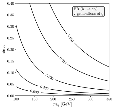
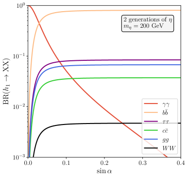
Figure 3: Branching ratios of the $h_{1}$ scalar into several final states for $n_{\eta}=2$, $\overline{\lambda}_{3}=0.55$, $\overline{\lambda}_{\eta S}\,v_{S}=500$ GeV and $\overline{\mu}_{\eta}=1500$ GeV. Left: contours of BR($h_{1}\to\gamma\gamma$) in the $m_{\eta}-\sin\alpha$ plane. Right: BR($h_{1}\to$ XX) as a function of $\sin\alpha$ for a fixed $m_{\eta}=200$ GeV.

We now show our numerical results. For the sake of simplicity, we will assume in the following that $\lambda_{3}$, $\mu_{\eta}$ and $\lambda_{\eta S}$ are proportional to the $n_{\eta}\times n_{\eta}$ identity matrix $\mathcal{I}_{n_{\eta}}$, that is, $X=\overline{X}\,\mathcal{I}_{n_{\eta}}$, with $X=\lambda_{3}$, $\mu_{\eta}$, $\lambda_{\eta S}$. Fig. 3 shows our results for the $h_{1}$ decay width and branching ratios into several final states. This figure has been made with the specific choice $n_{\eta}=2$, fixing also $\overline{\lambda}_{3}=0.55$, $\overline{\lambda}_{\eta S}\,v_{S}=500$ GeV and $\overline{\mu}_{\eta}=1500$ GeV. The left-hand side of this figure shows contours of BR($h_{1}\to\gamma\gamma$) in the $m_{\eta}-\sin\alpha$ plane. One can see that BR($h_{1}\to\gamma\gamma$) decreases with $m_{\eta}$, as expected, and gets enhanced for low values of $\sin\alpha$. In fact, the branching ratio into the diphoton final state can be of order $1$ for very low values of $\sin\alpha$. This behavior is also illustrated on the right-hand panel of the figure, which shows the dependence of the different BR($h_{1}\to$ XX) on $\sin\alpha$ for a fixed $m_{\eta}=200$ GeV. The enhancement is caused by the strong suppression of all the other channels, which have negligible branching ratios for low values of $\sin\alpha$. This is simply due to the fact that the $h_{1}\approx S$ decay into SM states can only take place via singlet-doublet mixing. It is important to notice that for values of $\sin\alpha\gtrsim 0.05$ the branching ratio to a $b\bar{b}$ pair becomes predominant favouring the LEP signal as was explained in Sec. 3.

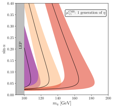
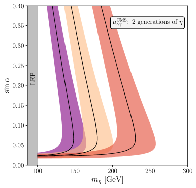
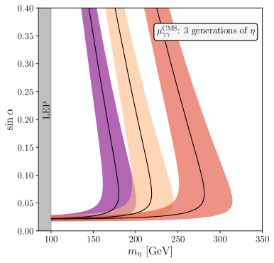
Figure 4: Regions of the $m_{\eta}-\sin\alpha$ plane that explain the CMS diphoton excess for fixed values of $\overline{\lambda}_{\eta S}\,v_{S}=500$ GeV and $\overline{\lambda}_{3}=0.6$. The colored regions accommodate $\mu^{\rm CMS}_{\gamma\gamma}$ at $1\,\sigma$, while the solid lines correspond to the CMS central value $\mu^{\rm CMS}_{\gamma\gamma}=0.33$. The different colors are associated to different values of $\overline{\mu}_{\eta}=$ 500 GeV (purple), 1000 GeV (yellow), 2000 GeV (red). The gray band on the left is (in principle) excluded by direct searches at LEP, although it would be allowed for sufficiently compressed spectra.

Fig. 4 displays different examples that prove that our model can easily fit the CMS diphoton excess. In order to obtain these solutions we have assumed the coupling of the $\eta$ scalars to the $h_{1}$ and $h_{2}$ scalars to be $\overline{\lambda}_{\eta S}\,v_{S}=500$ GeV and $\overline{\lambda}_{3}=0.6$, respectively, and we also fixed the value of $\overline{\mu}_{\eta}$ in the three figures to 500 GeV (purple regions), 1 TeV (yellow regions), and 2 TeV (red regions). Then, we found the $(m_{\eta},\sin\alpha)$ pairs that can reproduce $\mu_{\gamma\gamma}^{\rm CMS}$. Furthermore, we also vary the number of $\eta$ generations in the model and assume degenerate $\eta$ doublets. The upper left plot of Fig. 4 represents the solution for only one generation of $\eta$ doublets. We can see that the $m_{\eta}$ range in which our model explains the CMS diphoton excess depends on the values of $\mu_{\eta}$. For example, for the lowest value of the coupling, $\overline{\mu}_{\eta}=500$ GeV, the mass of the charged $\eta$ scalars must be around $m_{\eta}\sim 100$ GeV to compensate the low value of the parameter, whereas for larger values of the coupling the $\eta$ masses can reach $\sim 180$ GeV. In the upper right plot of Fig. 4 we can see the case of 2 generations of $\eta$ that have the same mass $m_{\eta_{1}}=m_{\eta_{2}}=m_{\eta}$. With two generations, the diphoton rate increases and, for this reason, the CMS diphoton excess is explained for greater values of the $\eta$ mass. Something similar happens in the case of 3 generations, shown in the lower pannel of Fig. 4. In this case, the $m_{\eta}$ value required to accommodate the CMS excess can be as high as 300 GeV when the $\mu_{\eta}$ couplings are of the order of 2 TeV.

It is important to note that an explanation for the CMS diphoton excess can be found for small values of $\sin\alpha$, in the $\sim 0.02$ ballpark. This may be surprising at first, since such low values of the singlet-doublet mixing angle strongly suppress the production of $h_{1}$ at the LHC. However, the existence of the low $\alpha$ region is due to the abovementioned increase in BR($h_{1}\to\gamma\gamma$), see Fig. 3, which compensates for the reduction in the production cross section. In fact, one can estimate a lower limit on $\sin\alpha$, below which $h_{1}$ cannot fit the CMS diphoton signal strength because the required branching ratio into $\gamma\gamma$ would be larger than 1. The production cross section for a SM Higgs that decays into a pair of photons at $\sqrt{s}=$ 13 TeV is approximately $\sigma_{H}\times\text{BR}(H\to\gamma\gamma)\sim 0.125\,{\rm pb}$ [7]. Then, assuming the hypothetical scenario with $\text{BR}(h_{1}\to\gamma\gamma)\to 1$ one finds the limit $\sin\alpha\gtrsim 0.0215$ for the central value of $\mu^{\rm CMS}_{\gamma\gamma}$ and the range $\sin\alpha\gtrsim[0.027-0.017]$ taking the $1\,\sigma$ region. This is precisely what determines the low $\alpha$ region observed in Fig. 4.

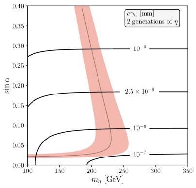
Figure 5: Contours of $\Gamma_{h_{1}}$ (in GeV) in the $m_{\eta}-\sin\alpha$ plane for a variant of the model with 2 generations of $\eta$ doublets. The colored region explains the CMS diphoton excess at $1\,\sigma$ with 2 generations of $\eta$, $\overline{\lambda}_{\eta S}v_{s}=500$ GeV, $\overline{\mu}_{\eta}=2000$ GeV and $\overline{\lambda}_{3}=0.6$.

Given that some regions of the $m_{\eta}-\sin\alpha$ plane considered in Fig. 4 have small $\sin\alpha$ values, one may wonder about the decay width of $h_{1}$. We note that $h_{1}$ must decay promptly for our explanation of the CMS diphoton excess to work. We explore this in Fig. 5, which shows contours of $c\tau_{h_{1}}$ in the $m_{\eta}-\sin\alpha$ plane for a variant of our model featuring 2 generations of $\eta$ doublets. We see that $h_{1}$ has a short decay length, well below that regarded as prompt, even for small $\alpha$ angles. Again, the reason is the enhancement of the diphoton decay channel.

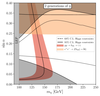
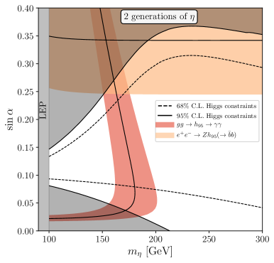
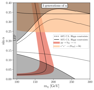
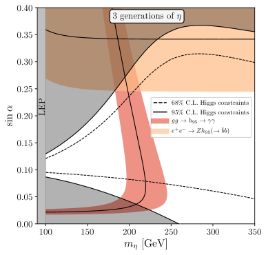
Figure 6: Regions of the $m_{\eta}-\sin\alpha$ plane that explain the CMS diphoton and LEP $b\bar{b}$ excesses. The region that explains the CMS diphoton excess at $1\,\sigma$ is shown in light red for $n_{\eta}=2$ (top panels) and $3$ (bottom panels). We have fixed $\overline{\lambda}_{S\eta}\,v_{S}$= 500 GeV and $\overline{\lambda}_{3}=0.6$, while the trilinear $\overline{\mu}_{\eta}$ takes the values 500 GeV (left panels) and 1000 GeV (right panels). The area that fits the LEP excess in $b\bar{b}$ is shown as light orange while we show as a dark gray shaded contour the area that is disfavoured at $95\%$ C.L. by Higgs constraints.

Let us now consider the LEP $b\bar{b}$ excess in combination with the previously discussed CMS diphoton excess. One can see in Fig. 6 the region of the $(m_{\eta},\sin\alpha)$ plane where both excesses can be explained. As discussed in Sec. 3, the charged $\eta$ scalars not only affect the $h_{1}$ diphoton rate, but also modify the one for $h_{2}$, already measured at the LHC. This implies limits from Higgs data, displayed in this figure by the dark gray area, which is excluded at $95\%$ C.L.. One should notice that the LEP excess can be explained in a region of parameter space that lies on a high value of $\sin\alpha$ and is mostly excluded by Higgs data. However, there is still a portion of the allowed parameter space where both excesses are explained. As expected, this portion involves lighter charged $\eta$ scalars when fewer generations are considered. With the specific values chosen in this figure for the $\overline{\lambda}_{S\eta}\,v_{S}$, $\overline{\lambda}_{3}$ and $\overline{\mu}_{\eta}$ parameters, the required $\eta$ masses range from $\sim 130$ GeV to $\sim 220$ GeV. Finally, we note that the dark gray area in Fig. 6 depends very strongly on the $\overline{\lambda}_{3}$ value. This can be easily understood by inspecting Eq. (23). For some values of $\overline{\lambda}_{3}$, the $g_{h_{2}\eta\eta}$ coupling becomes $\mathcal{O}(1)$ and excludes most of the parameter space due to Higgs data. However, one can choose specific values of $\overline{\lambda}_{3}$ that induce a cancellation in the $g_{h_{2}\eta\eta}$ coupling and make the constraints from Higgs data less stringent. Our choice $\overline{\lambda}_{3}=0.6$ is an example of this.

Alternatively, since the LEP $b\bar{b}$ excess is not very significant from a statistical point of view, one can interpret it as an upper limit on the $e^{+}e^{-}\to Z\,h_{95}\to Zb\bar{b}$ cross section. In this case, we conclude that the restrictions imposed by the LEP search in this channel are compatible with the areas where our model can explain the diphoton excess in CMS. The case of the CMS ditau excess is similar. The value of $\sin\alpha$ that would be required to explain this excess is quite large, above the current limit. The minimum value of the mixing angle in order to explain this signal would be $\sin\alpha_{\rm{min}}\sim 0.7$. However, as there is only one search by CMS at still low luminosity and there are no more searches, we consider this excess as still not significant. We can again interpret it as an upper bound on the $pp\to\,h_{95}\to\tau^{+}\tau^{-}$ cross section. In this case, we conclude again that the region of parameter space where the CMS diphoton excess is explained respects this bound.

6 Discussion

Once shown that our scenario can accommodate the 95 GeV anomalies, let us comment on some other aspects of the model that have been ignored in our previous discussion. This is the case of neutrino oscillation data. As already explained in Sec. 2.3, neutrinos acquire non-zero masses via loops involving the $\mathbb{Z}_{2}$-odd states $N_{n}$ and $\eta_{a}$. Therefore, the resulting neutrino mass matrix depends on their masses, as well as on the $\lambda_{5}$ quartics and the $y$ Yukawa couplings [37]. For specific values of $n_{N}$ and $n_{\eta}$, the $y$ Yukawa couplings can be readily written in terms of the parameters measured in oscillation experiments using a Casas-Ibarra parametrization [59] adapted to the Scotogenic model [60, 61, 62]. However, we note that the $y$ Yukawa couplings do not play any role in the 95 GeV collider phenomenology.

The Scotogenic variant discussed here also contains a DM candidate. In this family of models one usually has two options: fermion ($N_{1}$) or scalar ($\eta_{1}^{0}$) DM. However, in order to accommodate the 95 GeV anomalies we require relatively light $\eta$ doublets, with masses $m_{\eta}\lesssim 300$ GeV for $n_{\eta}\leq 3$.  This is too light to accommodate the DM relic density determined by the Planck collaboration [63]. In fact, the scalar DM scenario resembles the Inert Doublet Model [64], which is known to fully account for the observed relic density for DM masses in the $500-700$ GeV range [53, 65, 66, 67]. In contrast, $m_{\eta}\lesssim 300$ GeV leads to underabundant DM, hence requiring an additional DM component. We should also note that we consider more than one generation of $\eta$ doublets. This variation of the Scotogenic model deserves further investigation, since it may lead to novel possibilities in scenarios with scalar DM. Alternatively, we may consider scenarios with fermion DM. This candidate is known to be potentially problematic due to existing tension between the DM relic density (which requires large $y$ Yukawas) and contraints from lepton flavor violating observables (which require small $y$ Yukawas), see for instance [68]. Two interesting scenarios emerge:

• $m_{N_{1}}\ll m_{\eta_{1}^{0}}$. If the DM particle $N_{1}$ is much lighter than the $\eta$ states (for instance, $m_{N_{1}}\sim 100$ GeV and $m_{\eta_{1}}\sim 300$ GeV), the $y$ Yukawa parameters must be fine-tuned to suppress the contributions to $\mu-e$ flavor violating processes, such as $\mu\to e\gamma$, while being compatible with neutrino oscillation data. Although tuned, this scenario is possible. It would be characterized at the LHC by the pair production (due to the $\mathbb{Z}_{2}$ symmetry) of $\eta$ states which subsequently decay into the invisible $N_{1}$ and leptons: $\eta_{1}^{0}\to N_{1}\,\nu$ and $\eta_{1}^{\pm}\to N_{1}\,\ell^{\pm}$. This scenario is constrained by existing searches for sleptons, which would have a very similar phenomenology in both R-parity conserving and violating supersymmetry (see for instance [69, 70, 71, 72]). Furthermore, a light $N_{1}$ may also contribute to the invisible decay of $h_{1}$ (if $m_{N_{1}}\leq m_{h_{1}}/2$) and/or $h_{2}$ (if $m_{N_{1}}\leq m_{h_{2}}/2$). In fact, the $h_{1}\to N_{1}N_{1}$ invisible channel may easily dominate the $h_{1}$ decay width and preclude an explanation of the 95 GeV excess.

• $m_{N_{1}}\lesssim m_{\eta_{1}^{0}}$. If the $N_{1}$ singlet is almost degenerate with the lightest $\eta$ states, coannihilations become efficient and the DM relic density is more easily obtained. This enlarges the viable parameter space of the model and leads to novel signatures at the LHC. If the mass splitting $\Delta m=m_{\eta_{1}^{\pm}}-m_{N_{1}}$ is small enough, the decay $\eta_{1}^{\pm}\to N_{1}\,\ell^{\pm}$ may involve a long decay length, hence producing charged tracks at the detector.

Finally, in parameter points with $m_{N_{1}}\approx m_{h_{i}}/2$ the annihilation cross section in the early universe gets enhanced due to resonant effects. In such cases one can achieve the correct DM relic density without invoking large couplings. This is a generic feature that does not affect the previous discussion.

7 Summary and conclusion

We have shown that a theoretically well-motivated and economical model can accommodate the diphoton excess hinted by CMS and ATLAS at 95 GeV as well as the hint for a $b\bar{b}$ excess at similar energies by LEP. Our model is a minimal extension of the Scotogenic model and, besides addressing these collider anomalies, also provides a mechanism for the generation of neutrino masses and a testable dark matter candidate. We have allowed for variable numbers of generations of the Scotogenic states $N$ and $\eta$ and discussed our results for several choices of interest.

Two CP-even (and $\mathbb{Z}_{2}$-even) scalars: $h_{1}$ and $h_{2}$. The lightest of these states, $h_{1}$, is identified with $h_{95}$, the hypothetical scalar that is responsible for the $\gamma\gamma$ and $b\bar{b}$ excesses at 95 GeV, while $h_{2}$ is the Higgs-like state discovered by the CMS and ATLAS collaborations in 2012. Our numerical analysis shows that the excesses can be accommodated in our model in a large fraction of the parameter space. The viable region is characterized by sizable $\mu_{\eta}$ trilinear couplings and leads to $\eta$ scalars with masses below $\sim 300$ GeV ($\sim 180$ GeV) for $n_{\eta}=3$ (for $n_{\eta}=1$). As expected, a larger number of $\eta$ generations implies larger contributions to the $h_{1}$ diphoton coupling and enlarges the viable parameter space.

Our scenario has a rich phenomenology, both at colliders and at low-energy experiments. The nature of the dark matter candidate and the particle spectrum determines the phenomenology at colliders. Depending on the mass differences between the lightest $\mathbb{Z}_{2}$-odd fermion and $\mathbb{Z}_{2}$-odd scalar, one expects monolepton events including missing energy or charged tracks at the LHC detectors. In addition, the usual lepton flavor violating signatures, common to most low-energy neutrino mass models, are expected too. Therefore, our setup not only is well motivated from a theoretical point of view, but also has interesting phenomenological implications.

We conclude with a note of caution. Although the coincidence of several excesses, hinted by independent experiments at the same invariant mass, is highly intriguing, their relatively low statistical significance implies that more data is required to fully assess their relevance. We eagerly look forward to future updates on the 95 GeV excesses.

Appendix A Loop functions

The loop functions involved in the calculation of $\Gamma(h_{i}\to\gamma\gamma)$ are given by [38, 39, 40]

$$A_{0} =-[\tau-f(\tau)]/\tau^{2}\,,$$

$$A_{1/2} =2[\tau+(\tau-1)f(\tau)]/\tau^{2}\,,$$ (29)

$$A_{1} =-[2\tau^{2}+3\tau+3(2\tau-1)f(\tau)]/\tau^{2}\,,$$

where the function $f(\tau)$ is defined as

$$f(\tau)=\left\{\begin{array}[]{lc}\arcsin^{2}\sqrt{\tau};&\tau\leq 1\\ \\ -\frac{1}{4}\left[\log\frac{1+\sqrt{1-\tau^{-1}}}{1-\sqrt{1-\tau^{-1}}}-i\pi\right]^{2};&\tau>1\end{array}\right.$$ (33)

References

- [1] OPAL Collaboration, G. Abbiendi et al., “Decay mode independent searches for new scalar bosons with the OPAL detector at LEP,” Eur. Phys. J. C 27 (2003) 311–329, arXiv:hep-ex/0206022.
- [2] LEP Working Group for Higgs boson searches, ALEPH, DELPHI, L3, OPAL Collaboration, R. Barate et al., “Search for the standard model Higgs boson at LEP,” Phys. Lett. B 565 (2003) 61–75, arXiv:hep-ex/0306033.
- [3] ALEPH, DELPHI, L3, OPAL, LEP Working Group for Higgs Boson Searches Collaboration, S. Schael et al., “Search for neutral MSSM Higgs bosons at LEP,” Eur. Phys. J. C 47 (2006) 547–587, arXiv:hep-ex/0602042.
- [4] CDF, D0 Collaboration, “Updated Combination of CDF and D0 Searches for Standard Model Higgs Boson Production with up to 10.0 fb-1 of Data,” 7, 2012. arXiv:1207.0449 [hep-ex].
- [5] CMS Collaboration, “Search for new resonances in the diphoton final state in the mass range between 80 and 110 GeV in pp collisions at TeV,” tech. rep., CERN, Geneva, 2015. CMS-PAS-HIG-14-037.
- [6] CMS Collaboration, A. M. Sirunyan et al., “Search for a standard model-like Higgs boson in the mass range between 70 and 110 GeV in the diphoton final state in proton-proton collisions at 8 and 13 TeV,” Phys. Lett. B 793 (2019) 320–347, arXiv:1811.08459 [hep-ex].
- [7] CMS Collaboration, “Search for a standard model-like Higgs boson in the mass range between 70 and 110 in the diphoton final state in proton-proton collisions at ,” tech. rep., CERN, Geneva, 2023. CMS-PAS-HIG-20-002.
- [8] ATLAS Collaboration, “Search for resonances in the 65 to 110 GeV diphoton invariant mass range using 80 fb-1 of collisions collected at TeV with the ATLAS detector,” tech. rep., CERN, Geneva, 2018. ATLAS-CONF-2018-025.
- [9] CMS Collaboration, A. M. Sirunyan et al., “Search for additional neutral MSSM Higgs bosons in the final state in proton-proton collisions at 13 TeV,” JHEP 09 (2018) 007, arXiv:1803.06553 [hep-ex].
- [10] CMS Collaboration, “Searches for additional Higgs bosons and for vector leptoquarks in final states in proton-proton collisions at = 13 TeV,” arXiv:2208.02717 [hep-ex].
- [11] ATLAS Collaboration, “Search for boosted diphoton resonances in the 10 to 70 GeV mass range using 138 fb-1 of 13 TeV collisions with the ATLAS detector,” arXiv:2211.04172 [hep-ex].
- [12] S. Gascon-Shotkin, “Searches for additional higgs bosons at low mass,” in Talk at MoriondEW, CMS. 2023. indico.cern.ch.
- [13] C. Arcangeletti, “Measurement of higgs boson production and search for new resonances in final states with photons and z bosons with the atlas detector,” in CERN Seminar, ATLAS. 2023. CERN seminar.
- [14] A. Azatov, R. Contino, and J. Galloway, “Model-Independent Bounds on a Light Higgs,” JHEP 04 (2012) 127, arXiv:1202.3415 [hep-ph]. [Erratum: JHEP 04, 140 (2013)].
- [15] J. Cao, X. Guo, Y. He, P. Wu, and Y. Zhang, “Diphoton signal of the light Higgs boson in natural NMSSM,” Phys. Rev. D 95 no. 11, (2017) 116001, arXiv:1612.08522 [hep-ph].
- [16] ATLAS Collaboration, M. Aaboud et al., “Search for additional heavy neutral Higgs and gauge bosons in the ditau final state produced in 36 fb-1 of pp collisions at TeV with the ATLAS detector,” JHEP 01 (2018) 055, arXiv:1709.07242 [hep-ex].
- [17] P. J. Fox and N. Weiner, “Light Signals from a Lighter Higgs,” JHEP 08 (2018) 025, arXiv:1710.07649 [hep-ph].
- [18] F. Richard, “Search for a light radion at HL-LHC and ILC250,” arXiv:1712.06410 [hep-ex].
- [19] U. Haisch and A. Malinauskas, “Let there be light from a second light Higgs doublet,” JHEP 03 (2018) 135, arXiv:1712.06599 [hep-ph].
- [20] T. Biekötter, S. Heinemeyer, and C. Muñoz, “Precise prediction for the Higgs-boson masses in the SSM,” Eur. Phys. J. C 78 no. 6, (2018) 504, arXiv:1712.07475 [hep-ph].
- [21] F. Domingo, S. Heinemeyer, S. Paßehr, and G. Weiglein, “Decays of the neutral Higgs bosons into SM fermions and gauge bosons in the -violating NMSSM,” Eur. Phys. J. C 78 no. 11, (2018) 942, arXiv:1807.06322 [hep-ph].
- [22] D. Liu, J. Liu, C. E. M. Wagner, and X.-P. Wang, “A Light Higgs at the LHC and the B-Anomalies,” JHEP 06 (2018) 150, arXiv:1805.01476 [hep-ph].
- [23] J. M. Cline and T. Toma, “Pseudo-Goldstone dark matter confronts cosmic ray and collider anomalies,” Phys. Rev. D 100 no. 3, (2019) 035023, arXiv:1906.02175 [hep-ph].
- [24] T. Biekötter, M. Chakraborti, and S. Heinemeyer, “A 96 GeV Higgs boson in the N2HDM,” Eur. Phys. J. C 80 no. 1, (2020) 2, arXiv:1903.11661 [hep-ph].
- [25] J. A. Aguilar-Saavedra and F. R. Joaquim, “Multiphoton signals of a (96 GeV?) stealth boson,” Eur. Phys. J. C 80 no. 5, (2020) 403, arXiv:2002.07697 [hep-ph].
- [26] S. Heinemeyer and T. Stefaniak, “A Higgs Boson at 96 GeV?!” PoS CHARGED2018 (2019) 016, arXiv:1812.05864 [hep-ph].
- [27] S. Heinemeyer, “A Higgs boson below 125 GeV?!” Int. J. Mod. Phys. A 33 no. 31, (2018) 1844006.
- [28] T. Biekötter and M. O. Olea-Romacho, “Reconciling Higgs physics and pseudo-Nambu-Goldstone dark matter in the S2HDM using a genetic algorithm,” JHEP 10 (2021) 215, arXiv:2108.10864 [hep-ph].
- [29] T. Biekötter, A. Grohsjean, S. Heinemeyer, C. Schwanenberger, and G. Weiglein, “Possible indications for new Higgs bosons in the reach of the LHC: N2HDM and NMSSM interpretations,” Eur. Phys. J. C 82 no. 2, (2022) 178, arXiv:2109.01128 [hep-ph].
- [30] S. Heinemeyer, C. Li, F. Lika, G. Moortgat-Pick, and S. Paasch, “Phenomenology of a 96 GeV Higgs boson in the 2HDM with an additional singlet,” Phys. Rev. D 106 no. 7, (2022) 075003, arXiv:2112.11958 [hep-ph].
- [31] T. Biekötter, S. Heinemeyer, and G. Weiglein, “Mounting evidence for a 95 GeV Higgs boson,” JHEP 08 (2022) 201, arXiv:2203.13180 [hep-ph].
- [32] T. Biekötter, S. Heinemeyer, and G. Weiglein, “Excesses in the low-mass Higgs-boson search and the -boson mass measurement,” arXiv:2204.05975 [hep-ph].
- [33] T. Biekötter, S. Heinemeyer, and G. Weiglein, “The CMS di-photon excess at 95 GeV in view of the LHC Run 2 results,” arXiv:2303.12018 [hep-ph].
- [34] C. Bonilla, A. E. Cárcamo Hernández, S. Kovalenko, H. Lee, R. Pasechnik, and I. Schmidt, “Fermion mass hierarchy in an extended left-right symmetric model,” arXiv:2305.11967 [hep-ph].
- [35] D. Azevedo, T. Biekötter, and P. M. Ferreira, “2HDM interpretations of the CMS diphoton excess at 95 GeV,” arXiv:2305.19716 [hep-ph].
- [36] E. Ma, “Verifiable radiative seesaw mechanism of neutrino mass and dark matter,” Phys. Rev. D 73 (2006) 077301, arXiv:hep-ph/0601225.
- [37] P. Escribano, M. Reig, and A. Vicente, “Generalizing the Scotogenic model,” JHEP 07 (2020) 097, arXiv:2004.05172 [hep-ph].
- [38] A. Djouadi, “The Anatomy of electro-weak symmetry breaking. I: The Higgs boson in the standard model,” Phys. Rept. 457 (2008) 1–216, arXiv:hep-ph/0503172.
- [39] A. Djouadi, “The Anatomy of electro-weak symmetry breaking. II. The Higgs bosons in the minimal supersymmetric model,” Phys. Rept. 459 (2008) 1–241, arXiv:hep-ph/0503173.
- [40] F. Staub et al., “Precision tools and models to narrow in on the 750 GeV diphoton resonance,” Eur. Phys. J. C 76 no. 9, (2016) 516, arXiv:1602.05581 [hep-ph].
- [41] P. Bechtle, O. Brein, S. Heinemeyer, G. Weiglein, and K. E. Williams, “HiggsBounds: Confronting Arbitrary Higgs Sectors with Exclusion Bounds from LEP and the Tevatron,” Comput. Phys. Commun. 181 (2010) 138–167, arXiv:0811.4169 [hep-ph].
- [42] P. Bechtle, O. Brein, S. Heinemeyer, G. Weiglein, and K. E. Williams, “HiggsBounds 2.0.0: Confronting Neutral and Charged Higgs Sector Predictions with Exclusion Bounds from LEP and the Tevatron,” Comput. Phys. Commun. 182 (2011) 2605–2631, arXiv:1102.1898 [hep-ph].
- [43] P. Bechtle, O. Brein, S. Heinemeyer, O. Stal, T. Stefaniak, G. Weiglein, and K. Williams, “Recent Developments in HiggsBounds and a Preview of HiggsSignals,” PoS CHARGED2012 (2012) 024, arXiv:1301.2345 [hep-ph].
- [44] P. Bechtle, O. Brein, S. Heinemeyer, O. Stål, T. Stefaniak, G. Weiglein, and K. E. Williams, “: Improved Tests of Extended Higgs Sectors against Exclusion Bounds from LEP, the Tevatron and the LHC,” Eur. Phys. J. C 74 no. 3, (2014) 2693, arXiv:1311.0055 [hep-ph].
- [45] P. Bechtle, S. Heinemeyer, O. Stal, T. Stefaniak, and G. Weiglein, “Applying Exclusion Likelihoods from LHC Searches to Extended Higgs Sectors,” Eur. Phys. J. C 75 no. 9, (2015) 421, arXiv:1507.06706 [hep-ph].
- [46] P. Bechtle, D. Dercks, S. Heinemeyer, T. Klingl, T. Stefaniak, G. Weiglein, and J. Wittbrodt, “HiggsBounds-5: Testing Higgs Sectors in the LHC 13 TeV Era,” Eur. Phys. J. C 80 no. 12, (2020) 1211, arXiv:2006.06007 [hep-ph].
- [47] H. Bahl, V. M. Lozano, T. Stefaniak, and J. Wittbrodt, “Testing exotic scalars with HiggsBounds,” Eur. Phys. J. C 82 no. 7, (2022) 584, arXiv:2109.10366 [hep-ph].
- [48] H. Bahl, T. Biekötter, S. Heinemeyer, C. Li, S. Paasch, G. Weiglein, and J. Wittbrodt, “HiggsTools: BSM scalar phenomenology with new versions of HiggsBounds and HiggsSignals,” arXiv:2210.09332 [hep-ph].
- [49] P. Bechtle, S. Heinemeyer, O. Stål, T. Stefaniak, and G. Weiglein, “: Confronting arbitrary Higgs sectors with measurements at the Tevatron and the LHC,” Eur. Phys. J. C 74 no. 2, (2014) 2711, arXiv:1305.1933 [hep-ph].
- [50] O. Stål and T. Stefaniak, “Constraining extended Higgs sectors with HiggsSignals,” PoS EPS-HEP2013 (2013) 314, arXiv:1310.4039 [hep-ph].
- [51] P. Bechtle, S. Heinemeyer, O. Stål, T. Stefaniak, and G. Weiglein, “Probing the Standard Model with Higgs signal rates from the Tevatron, the LHC and a future ILC,” JHEP 11 (2014) 039, arXiv:1403.1582 [hep-ph].
- [52] P. Bechtle, S. Heinemeyer, T. Klingl, T. Stefaniak, G. Weiglein, and J. Wittbrodt, “HiggsSignals-2: Probing new physics with precision Higgs measurements in the LHC 13 TeV era,” Eur. Phys. J. C 81 no. 2, (2021) 145, arXiv:2012.09197 [hep-ph].
- [53] R. Barbieri, L. J. Hall, and V. S. Rychkov, “Improved naturalness with a heavy Higgs: An Alternative road to LHC physics,” Phys. Rev. D 74 (2006) 015007, arXiv:hep-ph/0603188.
- [54] A. Abada and T. Toma, “Electric dipole moments in the minimal scotogenic model,” JHEP 04 (2018) 030, arXiv:1802.00007 [hep-ph]. [Erratum: JHEP 04, 060 (2021)].
- [55] ATLAS Collaboration, “Search for direct pair production of sleptons and charginos decaying to two leptons and neutralinos with mass splittings near the -boson mass in TeV collisions with the ATLAS detector,” arXiv:2209.13935 [hep-ex].
- [56] CMS Collaboration, “Combined search for electroweak production of winos, binos, higgsinos, and sleptons in proton-proton collisions at 13 TeV,” tech. rep., CERN, Geneva, 2023. CMS-PAS-SUS-21-008.
- [57] ATLAS Collaboration, G. Aad et al., “Searches for electroweak production of supersymmetric particles with compressed mass spectra in 13 TeV collisions with the ATLAS detector,” Phys. Rev. D 101 no. 5, (2020) 052005, arXiv:1911.12606 [hep-ex].
- [58] CMS Collaboration, A. Tumasyan et al., “Search for supersymmetry in final states with two or three soft leptons and missing transverse momentum in proton-proton collisions at = 13 TeV,” JHEP 04 (2022) 091, arXiv:2111.06296 [hep-ex].
- [59] J. A. Casas and A. Ibarra, “Oscillating neutrinos and ,” Nucl. Phys. B 618 (2001) 171–204, arXiv:hep-ph/0103065.
- [60] T. Toma and A. Vicente, “Lepton Flavor Violation in the Scotogenic Model,” JHEP 01 (2014) 160, arXiv:1312.2840 [hep-ph].
- [61] I. Cordero-Carrión, M. Hirsch, and A. Vicente, “Master Majorana neutrino mass parametrization,” Phys. Rev. D 99 no. 7, (2019) 075019, arXiv:1812.03896 [hep-ph].
- [62] I. Cordero-Carrión, M. Hirsch, and A. Vicente, “General parametrization of Majorana neutrino mass models,” Phys. Rev. D 101 no. 7, (2020) 075032, arXiv:1912.08858 [hep-ph].
- [63] Planck Collaboration, N. Aghanim et al., “Planck 2018 results. VI. Cosmological parameters,” Astron. Astrophys. 641 (2020) A6, arXiv:1807.06209 [astro-ph.CO]. [Erratum: Astron.Astrophys. 652, C4 (2021)].
- [64] N. G. Deshpande and E. Ma, “Pattern of Symmetry Breaking with Two Higgs Doublets,” Phys. Rev. D 18 (1978) 2574.
- [65] L. Lopez Honorez, E. Nezri, J. F. Oliver, and M. H. G. Tytgat, “The Inert Doublet Model: An Archetype for Dark Matter,” JCAP 02 (2007) 028, arXiv:hep-ph/0612275.
- [66] L. Lopez Honorez and C. E. Yaguna, “The inert doublet model of dark matter revisited,” JHEP 09 (2010) 046, arXiv:1003.3125 [hep-ph].
- [67] M. A. Díaz, B. Koch, and S. Urrutia-Quiroga, “Constraints to Dark Matter from Inert Higgs Doublet Model,” Adv. High Energy Phys. 2016 (2016) 8278375, arXiv:1511.04429 [hep-ph].
- [68] A. Vicente and C. E. Yaguna, “Probing the scotogenic model with lepton flavor violating processes,” JHEP 02 (2015) 144, arXiv:1412.2545 [hep-ph].
- [69] D. Dercks, H. Dreiner, M. E. Krauss, T. Opferkuch, and A. Reinert, “R-Parity Violation at the LHC,” Eur. Phys. J. C 77 no. 12, (2017) 856, arXiv:1706.09418 [hep-ph].
- [70] H. K. Dreiner and V. M. Lozano, “R-Parity Violation and Direct Stau Pair Production at the LHC,” arXiv:2001.05000 [hep-ph].
- [71] E. Arganda, V. Martin-Lozano, A. D. Medina, and N. Mileo, “Potential discovery of staus through heavy Higgs boson decays at the LHC,” JHEP 09 (2018) 056, arXiv:1804.10698 [hep-ph].
- [72] E. Arganda, V. Martín-Lozano, A. D. Medina, and N. I. Mileo, “Discovery and Exclusion Prospects for Staus Produced by Heavy Higgs Boson Decays at the LHC,” Adv. High Energy Phys. 2022 (2022) 2569290, arXiv:2102.02290 [hep-ph].