Young Stellar Object Candidates in IC 417

Abstract

IC 417 is in the Galactic Plane, and likely part of the Aur OB2 association; it is $\sim$2 kpc away. Stock 8 is one of the densest cluster constituents; off of it to the East, there is a ‘Nebulous Stream’ (NS) that is dramatic in the infrared (IR). We have assembled a list of literature-identified young stellar objects (YSOs), new candidate YSOs from the NS, and new candidate YSOs from IR excesses. We vetted this list via inspection of the images, spectral energy distributions (SEDs), and color-color/color-magnitude diagrams. We placed the 710 surviving YSOs and candidate YSOs in ranked bins, nearly two-thirds of which have more than 20 points defining their SEDs. The lowest-ranked bins include stars that are confused, or likely carbon stars. There are 503 in the higher-ranked bins; half are SED Class III, and $\sim$40% are SED Class II. Our results agree with the literature in that we find that the NS and Stock 8 are at about the same distance as each other (and as the rest of the YSOs), and that the NS is the youngest region, with Stock 8 a little older. We do not find any evidence for an age spread within the NS, consistent with the idea that the star formation trigger came from the north. We do not find that the other literature-identified clusters here are as young as either the NS or Stock 8; at best they are older than Stock 8, and they may not all be legitimate clusters.

Version from

1 Introduction

IC 417 (also LBN 173.46-00.16 and SH 2-234) is a young cluster in the Galactic Plane, essentially in the direction of the Galactic anti-center ($l$=173.38°, $b=-$00.20°), and $\sim$2 kpc away. It has been thought to be part of the Aur OB2 association, though evidence is mixed (see, e.g., Marco & Negueruela 2016 and references therein).

IC 417 has gained some notoriety in astrophotography circles; when combined with NGC 1931 (to its southeast; not shown or considered here), it makes for a dramatic image, and is sometimes called “the Spider and the Fly.” There is a relatively dense cluster, called Stock 8 (Stock 1956), apparent in optical images, which appears to be nestled in a bubble of nebulosity particularly obviously in the infrared (IR); there is nebulosity extending from it off to the East in a region called the “Nebulous Stream” (Jose et al. 2008; hereafter J08), which we abbreviate “NS.” In the mid-infrared, it is particularly impressive; see Figure 1, where there are clusters of red objects apparently embedded in the nebulosity. It is not entirely clear what the sequence of star formation is in this region, for example, how (or even whether) the star formation has been triggered (see, e.g., J08; Camargo et al. 2012; Dewangan et al. 2018). Towards that end, it is useful to identify the cluster members.

Young stellar objects (YSOs) can be identified from infrared (IR) excess from a circumstellar disk; ultraviolet (UV) or even blue excess from accretion; H$\alpha$ excess from accretion and/or coronal emission; variability at nearly any wavelength; and/or from clustering on the sky. All of these methods have been used to identify YSO candidates in this region, but relatively few studies have focused narrowly just on IC 417 and the region immediately surrounding it. Since IC 417 is in the Galactic Plane, it has been serendipitously observed by many surveys, but few articles have pulled together data from a variety of optical and IR instruments and focused on the stellar population as we do here. We now summarize what work has been done to date in this region.

The distance to IC 417 has fluctuated near $\sim$2 kpc. Mayer & Macak (1971) estimated 2.97 kpc; Fich & Blitz (1984) deduced a kinematic distance of 2.3 $\pm$0.7 kpc. Malysheva (1990) estimated 1.897 kpc, the closest distance estimate available. Mel’Nik & Efremov (1995) derived 2.68 kpc. J08 obtained 2.05$\pm$0.1 kpc, with the most detailed analysis to that point, based on optical and infrared data. Camargo et al. (2012) obtained 2.7 kpc, and placed it in the near side of the Perseus arm, with stellar ages $<$10 Myr. Marco & Negueruela (2016; hereafter MN16) estimated that the stars were 4-6 Myr and at a distance of 2.80${}^{+0.27}_{-0.24}$ kpc. Finally, Dewangan et al. (2018) estimate 2.8 kpc. Several authors (including J08; Camargo et al. 2012; Dewangan et al. 2018) have attempted to assemble a story of star formation across the region, with most concluding that there is some sequential and/or triggered star formation here, but the details of this have been difficult to pin down due to varying distance estimates for subsets of this region (including the larger population of structures thought to be part of Aur OB2), and the likelihood that particularly in and around IC 417, the age uncertainty is likely comparable to any age gradient (Camargo et al. 2012). Most of the stars we consider in this paper are thought to be at about the same distance. We have adopted a distance estimate of $\sim$2 kpc, and accept as likely members anything between 1 and 3 kpc, but acknowledge that there is still uncertainty in this distance. (Also see App. A.)

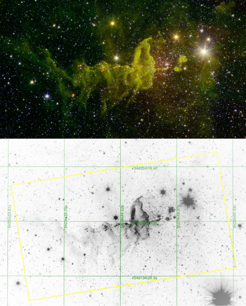
Figure 1: Top: three-color image of the heart of IC 417. Red=4.5 $\mu$m (from Spitzer/IRAC), green=3.6 $\mu$m (from Spitzer/IRAC), and blue=1.3 $\mu$m ($J$ band, from 2MASS). This image is a few degrees counter-clockwise of North-up, and it is about 0.5$\arcdeg$ across. Stock 8 is the cluster at the center-right, creating a ‘bowl’ in the green nebulosity. Clusters of red objects can be seen in the ‘nebulous stream’ in the center-left of this figure. (Image credit: NASA/JPL-Caltech, sig16-008.) Bottom: IRAC-2 (4.5 $\mu$m) image from GLIMPSE360 in reverse greyscale, north-up, showing sexigesimal coordinates (green) and the footprint of the media image (yellow). Also see next Figure.

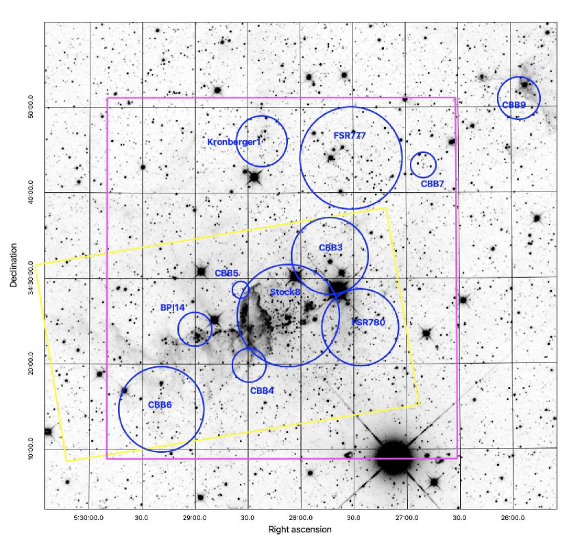
Figure 2: WISE-2 (4.5 $\mu$m; from unWISE) reverse greyscale image of our region. This image is $\sim$1$\arcdeg$ on a side, centered on 5:28:00 34:30:00 (J2000). The clusters from Figure 19 in C12 are included as indicated; see the text for more information. The clusters are listed in Table 1. The yellow polygon indicating the footprint from Fig. 1 is also shown for reference. The field we have focused upon is the magenta box, running from $\alpha,\delta$=05:26:31.5,+34:08:50.6 (the lower right corner of the magenta box) to 05:29:50,+34:51:05 (the upper left corner of the magenta box). (All coordinates are J2000).

Table 1: Literature Clusters in or near IC 417 (also see Fig. 2)

Name	Center (J2000)	Approx. Radius ($\arcsec$)	Notes
CBB 9	05:25:55 +34:50:54	150	Camargo et al. (2012); outside of the region considered in the rest of the paper
CBB 7	05:26:50 +34:43:10	90	Camargo et al. (2012)
FSR 777	05:27:31 +34:44:01	360	Froebrich et al. (2007); also Alicante 11 (MN16)
FSR 780	05:27:26 +34:24:12	270	Froebrich et al. (2007)
CBB 3	05:27:43.3 +34:32:36	270	Camargo et al. (2012)
Stock 8	05:28:07 +34:25:38	360	Stock (1956)
Kronberger 1	05:28:22 +34:46:01	180	Kronberger et al. (2006); also Alicante 12 (MN16)
CBB 4	05:28:29.3 +34:19:50	120	Camargo et al. (2012)
CBB 5	05:28:33.9 +34:28:37	60	Camargo et al. (2012)
BPI 14	05:29:00 +34:24:00	120	Borissova et al. (2003); also CC 14 (Ivanov et al. 2005); within the NS
CBB 6	05:29:19 +34:14:41.4	300	Camargo et al. (2012)

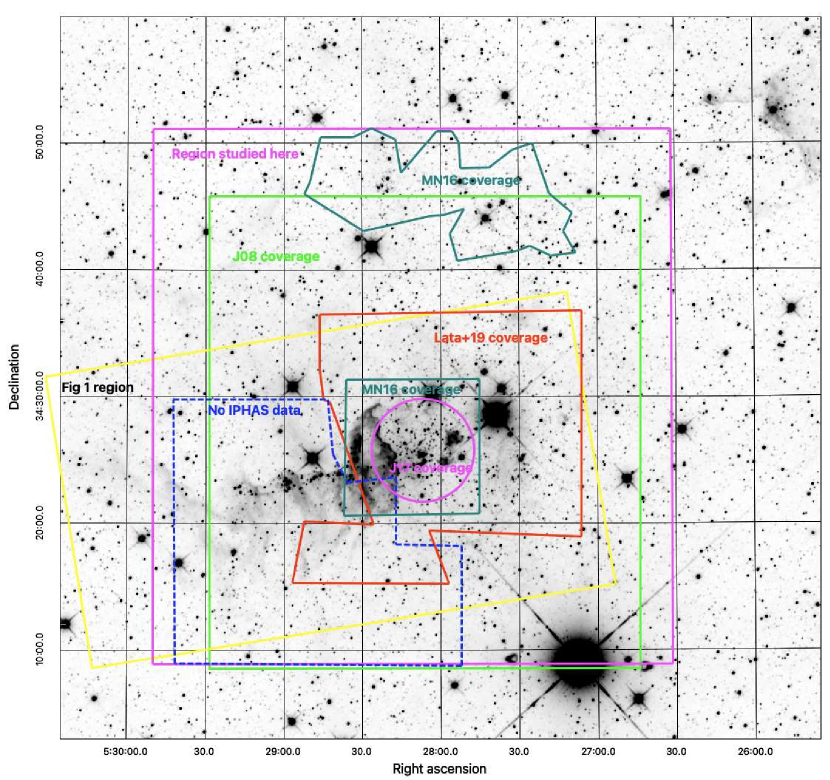
Figure 3: WISE-2 (4.5 $\mu$m) reverse greyscale image (as in Fig. 2) of our region, with yellow polygon (coverage of press image from Fig. 1) and large magenta square (our region of study) included for reference. The dark blue irregular polygon with dashed lines is the region that is NOT covered by IPHAS; note that it includes most of the NS. Green is J08 coverage; small teal square plus the irregular teal polygon to north is MN16; magenta circle is Jose et al. (2017); complex red polygon is Lata et al. (2019); UKIDSS coverage extends down to declination$\sim$34.25$\arcdeg$, which is about the lower edge of the red Lata et al. (2019) polygon. Many studies have focused on Stock 8 (see also Fig. 2); most of our work here is on the larger area, with a particular focus on the NS (see next Figure).

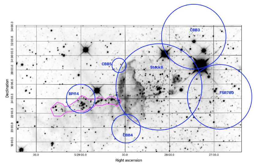
Figure 4: WISE-2 (4.5 $\mu$m) reverse greyscale image (from unWISE) of our region, zoomed in on the Nebulous Stream (NS). The blue clusters are as in Fig. 2, and only include the clusters entirely or mostly within this image. The magenta polygon is empirically derived here to include the regions of nebulosity and obviously red stars in Fig. 1.

The earliest work explicitly on the stars in this region dates from the 1970s-1980s and largely consists of identification of the brightest stars (Georgelin & Georgelin et S. Roux 1973; Vetesnik 1978; Efremov & Sitnik 1988; Chargeishsvili 1988). Malysheva (1990) also identified the brightest stars, and concluded the stars here were $\sim$12 Myr old. The brightest stars here are largely O and B stars, but include OP Aur, a carbon star. Additionally, Kohoutek & Wehmeyer (1999) noted some H$\alpha$-bright stars here.

The next significant advance in this region was with the release of the Two Micron All-Sky Survey (2MASS; Skrutskie et al. 2006). In the process of identifying clusters in various regions of the Galactic Plane, several authors used 2MASS-derived star count data to identify clusters in the IC 417 region. All the literature clusters in the IC 417 region are identified in Figure 2 and Table 1. Bica et al. (2003) called out the entire region, listing it as identical to IC 417. Borissova et al. (2003) identified BPI 14 (see Fig. 2 and Table 1). Ivanov et al. (2005) also called attention to BPI 14, labeling it CC 14. Kronberger et al. (2006) contributed the cluster marked Kronberger 1 in Fig. 2. Froebrich et al. (2007) identified FSR 777 and 780. Camargo et al. (2012) identified the clusters tagged “CBB” in Fig. 2 (and Table 1), in addition to confirming clusters from the literature, and providing the regional map on which our Fig. 2 is primarily based (see their Fig. 19). They find that all of these clusters are under 10 Myr old, all associated with each other, and most likely in the Perseus arm. An independent analysis by MN16 identified some of the same clusters from Camargo et al. (2012), to which they added additional deep Strömgren optical and new $JHK_{s}$ photometry, and some classification spectra (see Fig. 3 and Table 1). They confirmed clusters FSR 777 (which they call Alicante 11) and Kronberger 1 (which they call Alicante 12). They identify an O8 star (HD 35633) as the source of the ionizing photons carving out the ‘shell’ or ‘bowl’ around Stock 8 (Figs. 1 or 2), and an SB2 with integrated type O8 (BD+34$\arcdeg$1058) as the ionizing source to the north of the NS. They also reassessed the age and distance of the clusters in this region, finding 4-6 Myr and $\sim$2.80${}^{+0.27}_{-0.24}$ kpc, respectively. They suspect that it is in the Perseus arm, though possibly on the near side of it, noting that the location of the arm is not well-defined in this region. Interestingly, they find that the NS is not directly associated with Stock 8.

J08 was the first extensive survey of IC 417 itself (as opposed to as an additional cluster in a set of many). They included 2MASS data and deep optical ($UBVI_{c}$) imaging, and were primarily focused on the cluster Stock 8, which appears to sit within the “bowl” of nebulosity in Figs. 1 or 2. They identified near-infrared (NIR) excess and H$\alpha$ excess sources as candidate YSOs. They derived a distance of 2.05$\pm$0.1 kpc, and ages of 1-5 Myr. J08 is the first paper to identify the sinuous structure that is so obvious in the IRAC bands in Fig. 1. They found it in the NIR and dubbed it the “Nebulous Stream.” J08 conclude that the young clusters in the NS are at the same distance as Stock 8, but not yet affected by the star formation activity in Stock 8; instead, their formation was likely triggered by an O8 star to the North. The most prominent sub-cluster of the NS was identified as BPI 14 = CC 14 (Fig. 2 & Table 1).

Jose et al. (2017; hereafter J17) returned to Stock 8, analyzing the initial mass function of Stock 8 with deep optical, near-IR, and mid-IR data. They identified a “large, irregular cavity” at 350 $\mu$m and at 12 $\mu$m; IC 417 is at the southern edge of this cavity. They posit that the early-type stars identified in MN16 are creating this cavity, and that they have triggered star formation here, though not necessarily in Stock 8. They find that the NS is likely to be younger than Stock 8.

Dewangan et al. (2018) had an extensive discussion of the filamentary structures in IC 417 (which they call S234) as well as other clusters nearby in projected distance (which may or may not be part of Aur OB2). While largely focused on far-IR ($\geq$70 $\mu$m) and radio wavelengths and the distribution of gas/dust, a section of the paper includes figures with “selected YSOs,” however, no data table of the YSOs was provided. These authors are attempting to deduce the sequence of star formation in this region, and it is complicated at least in part because of the variety of estimated distances to the substructures of the complex. They also analyze the NS; they break the NS into two pieces. In Fig. 1, their “ns1” is the portion we consider to be the entirety of the NS, with the four subclusters of apparently red objects and the ‘sinuous’ texture of the nebulosity, parallel to the image orientation; their “ns2” is the far less prominent (more diaphanous) structure at about a 45$\arcdeg$ angle on the left. Dewangan et al. (2018) find far more interesting behavior in ns1; ns2 does not appear to be forming stars, whereas ns1 is forming, by their estimate, $\sim$80 YSOs (substantially fewer than we estimate here).

Lata et al. (2019) presented a variability analysis of stars in Stock 8, finding more than 100 short-period variables. They attribute many of the periodic signals they find to pulsation; they determine the age of their pre-main-sequence periodic variables to be $\lesssim$5 Myr. No analysis of the non-periodic variables is included in that paper. We chose to be more expansive and investigated all 130 periodic variables as possible YSO candidates, as opposed to just those identified as YSO candidates in Lata et al. (2019).

Pandey et al. (2020) explored star formation on a large scale in the larger Auriga region, of which IC 417 was just a part. They identified YSOs based on IR excess, finding two large bubble structures in the nebulosity and the YSO distribution; IC 417 is on the southern edge of one of their bubbles. They find far fewer YSOs North of IC 417 (within the bubble) than in or around it.

If the stars in the IC 417 region (including Stock 8, the NS, and the clusters discovered by star counts) are really $\sim$10 Myr old or as young as $\sim$3 Myr as some have claimed, at least $\gtrsim$10% of the member stars here should still have substantial circumstellar dust disks (e.g., Mamajek 2009). Exploring the disk fraction on the whole and as a function of location in this region may be able to provide constraints on the age (or age spread) of the clusters here. It is therefore worth looking for new YSO candidates based on IR excess. The stars in the NS are visibly red in Fig. 1. Given that there are numerous optical data sets available in this region, we should be able to determine if these stars are red primarily due to interstellar extinction or due to circumstellar dust. It is also worth exploring the clusters within the NS; four are evident by eye.

In this work, we collect the YSO candidates identified in the literature in this region, add objects apparently coincident with the NS, and add to that list new objects selected based on WISE+2MASS IR colors. We then investigate the optical+IR properties of this unified list of YSO candidates. We focus on a region from $\alpha,\delta$=05:26:31.5,+34:08:50.6 to 05:29:50,+34:51:05 (see Fig. 2; these coordinates are the lower right and the upper left corners of the magenta box in Fig. 2) because it covers most of the clusters identified here. We explore, where possible, the properties of the literature-identified clusters.

In Section 2, we present all the archival data we used, and how we merged the catalogs. Section 3 describes the assembly of the list of YSO candidates from the literature, by position in the NS, and via selection based on IR excess using 2MASS+WISE. Section 4 goes into detail of how we vetted the YSO candidates, using image inspection, SED inspection, color-magnitude and color-color diagram inspection, and our procedure for final ranking of the YSO candidates. In Section 5, we describe many properties of the entire ensemble of YSO candidates, and Section 6 delves into more detail about Stock 8 and the NS. Section 7 considers the OB and carbon stars in this region, and Section 8 explores the clusters found via 2MASS star counts. Section 9 summarizes our main results.

The Appendix has a variety of supporting information including more information on the distance to IC 417 (App. A), more on how we matched sources across catalogs (App. B), background information on how and where to find young stars in various color-color and color-magnitude diagrams (App. C), and then detailed examples of how we ranked a dozen sources out of our final YSO candidate list (App. D).

=1mm Band Wavelengths Resolution Limiting mag Origin Catalog YSO Candidate Color/symbol Notes ($\mu$m) ($\arcsec$) (mag) Fraction Fraction in SEDs $UBVI_{c}$ 0.36, 0.44, 0.55, 0.79 $\sim$3 17, 20, 19, 17 J08 15% 52% black + Published entire catalog, not just cluster members. Partial coverage, green box in Fig. 3. $uvby\beta$ 0.34, 0.41, 0.47, 0.55, 0.66 $\sim$0.7 17, 16, 15, 15, 2.8 MN16 0.5% 10% purple + Primarily bright stars. Partial coverage, cyan polygons in Fig. 3. $grizy$ 0.481, 0.617, 0.752, 0.866, 0.926 $\sim$0.6 22, 22, 20, 19.5, 19 Pan-STARRS 60% 84% cyan $\Diamond$ Covers whole region. $VI_{c}$ 0.44, 0.79 $\sim$0.7 21, 19 J17 3% 29% black + Partial coverage, magenta circle in Fig. 3. $r^{\prime},i^{\prime}$, H$\alpha$ 0.624, 0.774, 0.656 $\lesssim$0.9 18.7, 17.7, 15.3 IPHAS 32% 44% yellow $\Diamond$ Complex coverage, region that is NOT covered is the dark blue polygon in Fig. 3. $G_{BP},G_{p},G_{RP}$ 0.511, 0.622, 0.777 $\sim$0.4 20, 20, 19 Gaia DR2, DR3 45% 67% green $\Box$ Covers whole region; 26% have parallaxes from DR2 and 41% from DR3; 32% have distances from Bailer-Jones et al. (2018), and 41% from Bailer-Jones et al. (2021). $JHK_{s}$ 1.248, 1.631, 2.201 $\sim$1 16.5, 16, 15.5 UKIDSS 48% 85% red $\Diamond$ Covers most of the region, down to $\sim$34.25. $JHK_{s}$ 1.235, 1.662, 2.159 $\sim$1.6 16.7, 15.8, 15.4 2MASS 24% 71% black $\Diamond$ Covers whole region. $JHK_{s}$ 1.248, 1.631, 2.201 $\sim$2 16, 15.5, 15 MN16 1% 17% purple + Partial coverage, cyan polygons in Fig. 3. IRAC-1,2 3.6, 4.5 $\sim$1.6 15.2, 15.2 GLIMPSE 54% 91% black $\bigcirc$ highest spatial resolution and sensitivity available at these bands. Covers whole region. If source visible in image but not in GLIMPSE catalog, photometry taken from J17; yellow circles) or done anew here. WISE-1,2,3,4 3.4, 4.6, 12, 22 $\sim$6-12 14.6, 14.9, 12.3, 8.9 WISE 73% 58 % black $\star$ AllWISE release, plus CatWISE (blue $\Box$) and unWISE (green +). Covers whole region. MSX B1,B2, A, C, D, E 4.29, 4.35, 7.76, 11.99, 14.55, 20.68 $\sim$9-15 … MSX catalog $<$0.08% 1.4% cyan $\Box$ Too few points to assess limiting mag here ($<$40 sources). Covers whole region. AKARI IRC, FIS 9, 18; 65, 90, 140, 160 $\sim$2 … AKARI IRC, FIS $<$0.05% 1% yellow $\times$ Too few points to assess limiting mag here ($<$25 sources). Covers whole region. PACS 70,160 70, 160 5.6, 10.7 … PACS PSC $<$0.05% 0.7% green $\Box$ Too few points to assess limiting mag here ($<$25 sources). Covers whole region.

Table 2: Archival Data in IC 417

2 Data

2.1 Overview

In order to look for candidate YSOs in the IC 417 region, we first assembled data from a wide variety of places, summarized in Table 2, and discussed in this section. Because IC 417 is in the Galactic Plane, it has been serendipitously observed by several different surveys. Several data sets are available over our entire region (from $\alpha,\delta$=05:26:31.5,+34:08:50.6 to 05:29:50,+34:51:05; see Fig. 2), and some data are available only over a portion of the field (see Fig. 3). We kept track of the sources identified in the literature as YSOs or YSO candidates where relevant. In practice, we started with 2MASS to establish a reliable coordinate system and then found matches by position with sources from both shorter and longer wavelengths (see Sec. 2.5). Sources that were optical-only were not often retained unless they were listed in the literature as possible or confirmed YSOs.

All of these data were combined (bandmerged) initially by looking for matches by position, typically within 1$\arcsec$. Most of these catalogs have very good positions, so a larger radius is not required, except where specified below. After merging the catalogs, there are $\sim$46,000 objects, with data included from 0.34 to 160 $\mu$m. We used these catalogs to create spectral energy distributions (SEDs); see Sec. 4.2. By checking the SEDs, we can identify sources that are incorrectly bandmerged, because in those cases, the SEDs have obvious discontinuities. Those sources were given special attention and manually matched to the correct source as needed.

2.2 Optical

2.2.1 Pan-STARRS

Data from the Panoramic Survey Telescope and Rapid Response System (Pan-STARRS) DR1 (Chambers et al. 2016) were pulled from the Mikulski Archive for Space Telescopes (MAST) for this region. This survey covers this region in five bands ($grizy$) with a spatial resolution of $\sim$0.6$\arcsec$. In this region, this survey reaches $\sim$20th mag in most bands; see Table 2. We have Pan-STARRS counterparts for $\sim$60% of the sources in our master catalog of this region.

2.2.2 Gaia

Gaia DR2 (Gaia Collaboration 2018ab), EDR3 (Gaia Collaboration et al. 2021a,b), and DR3 (Gaia Collaboration 2022ab) data were obtained for this region via the Infrared Science Archive (IRSA; https://irsa.ipac.caltech.edu). The bands for this are $G,G_{BP},$ and $G_{RP}$; data go to $\sim$20th mag here. The effective wavelengths are slightly different between the two data releases. Gaia DR2 wavelengths for $G_{BP},G_{p},G_{RP}$ are 0.532, 0.673, & 0.797 $\mu$m, respectively, and E/DR3 wavelengths are 0.511, 0.622, & 0.777 $\mu$m. We have Gaia DR2 parallaxes for 26% of the master catalog, and 41% from DR3. Since some of the measured parallaxes are negative, we used distances from Bailer-Jones et al.; $\sim$32% have distances from Bailer-Jones et al. (2018), and $\sim$41% from Bailer-Jones et al. (2021). (Also see Appendix A on distances.) Data were collected and merged (by position) from DR2, EDR3, and DR3 because work for this project extended over enough years that data from all releases were relevant, and encompassed slightly different stars. In practice, the photometry and distances were matched by position and bookkept separately for each delivery, for each source.

2.2.3 IPHAS

The INT Photometric H$\alpha$ Survey (IPHAS; Barentsen et al. 2014) covered the Galactic plane in the Northern hemisphere, including the IC 417 region, in $r^{\prime},i^{\prime}$, and H$\alpha$. The spatial resolution of this survey is $\sim 1.1\arcsec$, and it goes to $\sim$17-19 mags in this region in the broadband filters. These data as served by VizieR (at least as of the time when we downloaded the catalog) are missing in a relatively large polygon in the SE of our field, over most of the NS (Fig. 3). According to J. Drew (2015, priv. comm.), this region was not observed on a photometric night and thus the photometry was not released as part of DR2. J. Drew kindly directly provided this lower-quality photometry in 2015, but for the stars that were detected in IPHAS, there are considerable other optical data available now, and there is a relatively large systematic offset (vividly apparent in the SEDs) between this lower-quality IPHAS data and the rest of the data we have amassed. Therefore, we did not use these lower-quality IPHAS data. There are good IPHAS counterparts for $\sim$32% of the sources in our catalog. Seventeen H$\alpha$-bright stars as identified in Witham et al. (2008) from this region were tagged as YSO candidates in our database.

2.2.4 J08

J08 published their entire catalog of $UBVI_{c}$ measurements, not just those for their candidate cluster members. This allows us to use their data for investigation of objects other than their candidate cluster members. Their spatial resolution is about $\sim$1.5$\arcsec$; their data cover only the central region (see Fig. 3). They include relatively faint objects; histograms of the measured magnitudes peak at $\sim$17-20 mag. In order to match correctly these optical measurements to the established catalog, sources were first matched by position to 2MASS, which revealed several duplicate sources and systematic offsets of reported positions of typically 0.5$\arcsec$, but with a long tail to larger separations that was strongly dependent on position on the sky. Individual sources were matched by hand (using tools and procedures developed in, e.g., Rebull 2015; see Appendix B) across surveys and across the field. In the end, 15% of our catalog had data from J08. Candidate cluster members from J08 were identified as candidate YSOs in our database.

2.2.5 MN16

MN16 published Strömgren photometry, as well as spectroscopy (specifically spectral types) in the central portion of the region and just north of it (see Fig. 3). Their scientific goals dictated that they focus on the O and B stars, so most of their objects are bright. Their resolution was $\sim 1\arcsec$, and we have counterparts from MN16 for just $\sim$6% of the final catalog. We incorporated all the reported photometry and spectral types from this work into our database. Stars that were O and B stars were identified as YSOs because stars that are that massive are at most a few million years old, and stars in the direction of and at the distance of IC 417 that are a few million years old are YSOs.

2.2.6 Spectral Types from the Literature

Spectral types from the literature (Georgelin & Georgelin et S. Roux 1973; Vetesnik 1978; Malysheva 1990; Efremov & Sitnik 1988; Chargeishsvili 1988) were included and all of the O and B stars were identified as YSOs in our database, matching by name rather than position.

2.2.7 J17

J17 returned to Stock 8 (alone; see Fig. 3), analysing the IMF of Stock 8 with deep optical data, which we included here. J. Jose kindly provided (priv. comm., 2018) the entire catalog, not just the YSOs. As for J08, these catalogs required a bit of manipulation to consolidate internal duplicates and adjust the astrometry to match 2MASS or Spitzer coordinates (see Appendix B). Just 3% of our catalog has a counterpart from J17.

2.2.8 Pandey et al. (2020)

Pandey et al. (2020) obtained observations in $VI$ over a very large region in Auriga; these optical observations were largely superseded by the optical data we already had amassed, so we retained solely the identification of YSO candidates from Pandey et al. (2020).

2.3 Near Infrared

2.3.1 2MASS

In 2MASS (Skrutskie et al. 2003, 2006), $JHK_{s}$ data in this region go to $\sim$15-17 mags, with a spatial resolution of $\sim$1.5$\arcsec$. The infrared data more easily penetrate the interstellar medium and can reveal stars not easily detected in the optical bands here. As described above, 2MASS provided the initial base catalog to which all other catalogs were merged (see Sec. 2.5 for more on the merging process). However, only $\sim$24% of our final, multi-wavelength merged catalog has a 2MASS match. The detections from the 2MASS catalog were only retained if the data quality flags were not D, E, F, or X. Upper limits were retained as such.

2.3.2 UKIDSS

The UKIRT Infrared Deep Sky Survey (UKIDSS) Galactic Plane Survey (Lucas et al. 2008) covered this region in $JHK_{s}$ to slightly fainter magnitudes than in 2MASS. At 0.8$\arcsec$, UKIDSS has higher spatial resolution than 2MASS. UKIDSS data are available over most of our field; its coverage includes the northern 90% of our field, to declination $\sim$34.25$\arcdeg$. About half our sources have UKIDSS counterparts.

2.3.3 MN16

MN16 published new $JHK_{s}$ photometry in the central portion of the region and just north of it, focusing on bright objects. The sensitivity of their $JHK_{s}$ data is comparable to, if not a little shallower than, the $JHK_{s}$ data from other sources. Their resolution was $\sim 1\arcsec$.

2.3.4 J17

J17, working in Stock 8 (alone) included near-IR data we have already included here (UKIDSS, 2MASS).

2.4 Mid- and Far-Infrared

2.4.1 WISE

The Widefield Infrared Survey Explorer (WISE; Wright et al. 2010a), like 2MASS, is an all-sky survey, so the IC 417 region was entirely included. The survey was conducted in four bands, 3.4, 4.6, 12, and 22 $\mu$m. We primarily used the AllWISE release (Wright et al. 2010b), which sums up all available data prior to 2011 February. The catalog reaches much fainter objects in the 3.4 and 4.6 $\mu$m than in 12 and 22 $\mu$m. However, the spatial resolution is relatively low, $\sim$6.1, 6.4, 6.5, and 12$\arcsec$ for the four channels, respectively. In this crowded region, the WISE sources often encompass more than one source seen at the shorter bands. However, because the Spitzer data (see below) do not go past 4.5 $\mu$m here, WISE is the best available choice for IR data between 5 and 25 $\mu$m. The detections from the AllWISE catalog were retained if the data quality flags were A, B, or C; if the data quality flag was Z, then the data were provisionally retained with a very large error bar, 30% larger than what appears in the catalog. Upper limits were retained as such.

The AllWISE catalog includes data prior to 2011 Feb, but far more data have been obtained from 2013 to date in WISE channels 1 and 2 (3.4 and 4.6 $\mu$m). CatWISE (Marocco et al. 2021, Eisenhardt et al. 2020, CatWISE team 2020) and unWISE (Lang 2014; Meisner et al. 2017a,b; Schlafly et al. 2019, Meisner et al. 2019) are both efforts to include these more recent data; both use images created by unWISE but obtain independent photometry. We included catalogs from both CatWISE and unWISE in our database; both cover the whole region. There is WISE photometry from at least one origin (AllWISE, CatWISE, unWISE) for 73% of the catalog.

Additionally, we had one more WISE data reduction. When we started this project, co-author Koenig had recently published papers with a new approach to identifying YSOs from WISE colors (Koenig & Leisawitz 2014 and Koenig et al. 2012). Koenig et al. (2012) describes an approach for doing photometry on WISE images, PhotVis. We had the output of PhotVis (and the YSO color selection) run on the AllWISE data. We only used the PhotVis photometry if there was not already photometry for that source at that band from AllWISE.

2.4.2 Spitzer

The Spitzer Space Telescope (Werner et al. 2004) program called Galactic Legacy Infrared Mid-Plane Survey Extraordinare (GLIMPSE; Churchwell et al. 2009) included the Galactic plane. The original GLIMPSE survey did not include IC 417, but the 2-band post-cryogen continuation of GLIMPSE late in the Spitzer mission called GLIMPSE360 did include this region (GLIMPSE team 2014; Meade et al. 2014), such that only the two shortest IRAC channels were used (3.6 and 4.5 $\mu$m). Nonetheless, the Spitzer data are more sensitive and are much higher spatial resolution ($\sim 1.2\arcsec$) than the WISE data, so they are very useful in this crowded region. GLIMPSE360 data are used in Fig. 1. For the catalogs, we used the ‘more complete, less reliable’ catalog (the GLIMPSE360 Archive); since we inspected each YSO candidate by hand (Sec. 4), it is more important that we get measurements of objects to as faint as possible, knowing that we can reject the less reliable detections on a case-by-case basis.

If the source could be seen in the IRAC images, but there was no corresponding row in the GLIMPSE360 catalog because it was just too faint, we performed standard aperture photometry on the GLIMPSE360 mosaics, as needed. (We used aperture 3 px, annulus 3-7 px, and aperture corrections 1.124 and 1.127, for IRAC-1 and -2, respectively; IRAC Instrument and Instrument Support Teams 2021.) J17 also used mid-IR (Spitzer/IRAC) imaging data from GLIMPSE360, doing their own photometry, but just in Stock 8. If no other photometry was available, we used the J17 IRAC photometry.

2.4.3 Winston et al. (2020)

Winston et al. (2020) used GLIMPSE360 data from Spitzer/IRAC combined with WISE and 2MASS data to select YSO candidates along the Galactic Plane (e.g., not just in this region). Since we already have the Spitzer, WISE, and 2MASS data in our database, we simply tagged their identified YSO candidates in our database.

2.4.4 AKARI

We also included AKARI (Murakami et al. 2007, AKARI team 2010a) IRC data at 9 and 18 $\mu$m for stars in this region. AKARI was an all-sky Japanese mission, but was not as sensitive as Spitzer, so only a handful of stars in our region have AKARI IRC counterparts (see Table 2). AKARI data required a 3$\arcsec$ matching radius to find counterparts.

2.4.5 Other Long Wavelength Data

There are long wavelength imaging data in this region, including AKARI FIS (50-180 $\mu$m; AKARI team 2010b), MSX (8-21 $\mu$m; Egan et al. 2003), and Herschel (Pilbratt et al. 2010) PACS (70-160 $\mu$m; Poglitsch et al. 2010; Marton et al. 2017) and SPIRE (250-500 $\mu$m; Griffin et al. 2010). Many of these datasets have been used in the literature (e.g., J17, Pandey et al. 2020, Dewangan et al. 2018). However, the long-wavelength data for point sources are prohibitively complicated for us to use because of the relatively low spatial resolution, relatively high source surface density, and relatively bright nebulosity. We matched our sources to most of these catalogs (all except SPIRE), usually with large matching radii (AKARI:3$\arcsec$; MSX:10$\arcsec$; Herschel:2$\arcsec$), but only retained the match if the SED made physical sense, if the given measurements were consistent (e.g., WISE, AKARI, and MSX all agreed), and/or if the source was not obviously confused. Correctly apportioning fractional long-wavelength flux among nebulosity and individual constituent point sources is beyond the scope of the present work. There were very few point sources that had counterparts in these long-wavelength catalogs.

2.5 Merging Catalogs

In order to merge catalogs, we started first with the largest near-IR catalogs because we knew that they would establish a high-reliability coordinate system to which we could link the rest of the sources, and that we were likely going to be primarily interested in those sources detected in the near-IR. Especially since we were unlikely to be interested in very many sources that were detected only in the optical, we retained (in contrast) relatively few sources that were detected only in the optical. Typically, we used 1$\arcsec$ as the matching radius. All three of the first catalogs (2MASS, GLIMPSE, WISE) should have high-quality astrometry all on the same coordinate system, and, when merged, provide a good anchor for merging the rest of the sources.

We merged catalogs in the following order: (1) 2MASS, retaining all detections; (2) GLIMPSE360 Archive (more complete but less reliable catalog), retaining all detections; (3) AllWISE, retaining all detections; (4) CatWISE, retaining all detections; (5) unWISE, retaining all detections; (6) WISE data from PhotVis and X. Koenig, retaining all detections; (7) PanSTARRS, retaining all detections whether or not there was an IR counterpart; (8) UKIDSS, dropping sources that have no counterpart in the catalog to this point; (9) IPHAS, dropping sources that have no counterpart in the catalog to this point; (10) Gaia DR2 & DR3 and associated distances from Bailer-Jones et al. (2018, 2021), dropping sources that have no counterpart in the catalog to this point; (11) Herschel/PACS, dropping sources that have no counterpart in the catalog to this point; (12) AKARI IRC, dropping sources that have no counterpart in the catalog to this point; (13) MSX, dropping sources that have no counterpart in the catalog to this point; (14) J08 data, pre-matched to 2MASS as described above, including ancillary information; (15) J17, including ancillary information, all of which have matches in the assembled catalog to this point; (16) spectral types and YSO identifications from references not already included were then matched by target position.

What this process means in detail is the following. We started with 2MASS, then looked for matches between Spitzer/GLIMPSE360 and 2MASS. Targets that had matches in GLIMPSE360 had their GLIMPSE360 fluxes matched to their 2MASS entries, and then the GLIMPSE360-only sources were added to the master catalog as new sources (“retaining all detections”), using their GLIMPSE360 positions and fluxes. Because the coordinate system is the same between 2MASS and Spitzer, this is not a significant source of error. Then, we looked for matches between the merged 2MASS+GLIMPSE360 master catalog and AllWISE. When a match is found, the AllWISE fluxes are matched to the master catalog entries. After the matching, the AllWISE-only sources are added to the master catalog as new sources using the WISE positions and fluxes (“retaining all detections”). The coordinate system is the same among 2MASS/Spitzer and WISE. The process is repeated in the order as specified above, for each of the items 1-6; these are infrared catalogs, all on the same coordinate system. Item 7 is the first optical catalog to be merged, PanSTARRS. For this optical catalog, the same process was imposed – look for matches between PanSTARRS and the master catalog, copy the PanSTARRS measurements over to the counterpart’s entry, and finish by including the PanSTARRS-only sources into the master catalog with their PanSTARRS positions and brightnesses. However, for catalogs after this point, we discovered empirically that the errors imposed by concatenating new sources on different coordinate systems added more “noise than signal” – e.g., the chances were much higher of adding false sources or sources that were offset enough from their ‘true’ position such that finding their counterpart by doing blind position matching to subsequent catalogs was substantially harder. Because our scientific interest is largely focused on the IR-bright sources, we did not retain sources for which there was no match in the master catalog after item 7 (“dropping sources that have no counterpart in the catalog to this point”). The exception to this is any source that was identified independently as an ‘interesting’ source in the literature. Those were explicitly included in the master catalog.

After item 16, there are $\sim$46,000 objects in the merged catalog, including wavelengths from 0.34 to 160 $\mu$m, with up to 58 measurements at up to 47 distinct wavelengths, though few objects have detections across all bands even just 0.34 to 22 $\mu$m, much less out to 160 $\mu$m.

In order to get a best possible measurement in the near-IR $JHK_{s}$ bands, we took first measurements from 2MASS, then those from UKIDSS, then from MN16. We used (and tabulated) the best possible $JHK_{s}$ detections for calculations as described below; values from 2MASS, UKIDSS, and MN16 are also tabulated separately in our catalog.

As discussed in Sec. 4.2 below, when we were checking each source’s images and SED, if there were unphysical discontinuities, we returned to the merging process, unlinked incorrect matches, and made correct matches where possible. In some cases, it was not obvious which data set was wrong, and in those cases, we left them all tied to the source; those will be obvious to the reader when inspecting the SEDs, but they include those with rank ‘1r’ or ‘4*’ (see Sec. 4.4).

3 Identifying YSO candidates

3.1 Overview

We assembled our list of YSOs and YSO candidates primarily in three ways: (1) literature lists of YSOs/candidates; (2) selection by position in the NS; (3) selection by IR excess using 2MASS+WISE. This section describes each of these approaches.

Table 3 collects all the total numbers (and fractions) of stars in the final sample (omitting the sources ultimately rejected in Sec. 4). Table 4 has all of the YSOs that survived the analysis described in this paper, and has also been delivered to IRSA (along with individual SEDs for each object). Figure 5 shows where the stars are on the sky, with the clusters from Fig. 2 for reference.

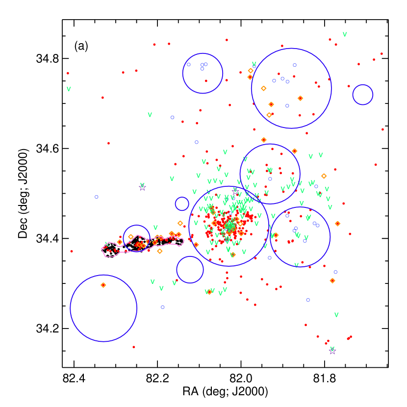
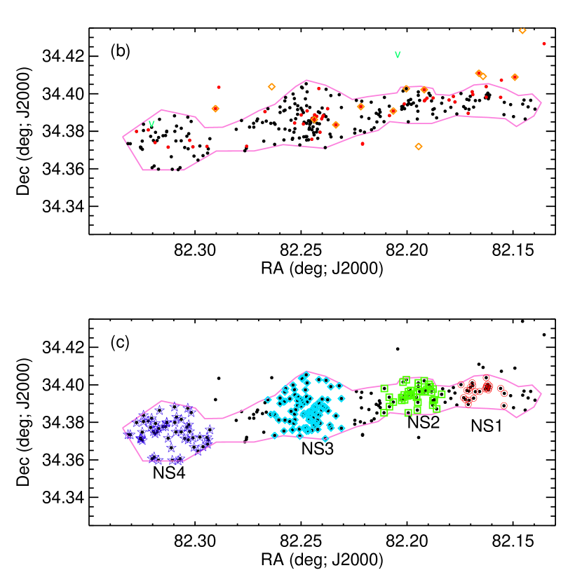
Figure 5: (a): Location of the YSO candidates on the sky, with the clusters from Table 1 and Fig. 2. Red filled circle: stars identified in the literature or here via WISE as having an IR excess; blue open circle: stars identified in the literature as an O or B star; green v: stars identified in the literature as variable; orange open diamond: stars identified in the literature as H$\alpha$-bright; purple open stars: carbon stars from the literature; filled black dots: stars identified here as part of the NS. (b): zoom-in on the NS, with same symbols as the first plot, with the boundaries of the NS as the magenta polygon. (c): zoom-in on the NS, with magenta polygon, but this time different subclusters defined as indicated, numbered in order of increasing RA. Black dots are just stars in the catalog; additional red circle=subcluster 1, green square=subcluster 2, cyan diamonds=subcluster 3; purple star=subcluster 4. Subcluster 3 has substantial overlap with the BPI14 literature cluster. Our YSO candidate list is biased towards stars in Stock 8 and NS because of the way we constructed the list – many of the literature YSOs are in Stock 8 because that was the focus of those studies. We defined the boundaries of the NS, so it is readily apparent in the first plot. The right plot defines possible subclusters within the NS for use later in the paper; note that some stars in the NS are not assigned to a subcluster.

Table 3: Total Number YSO Candidates In or Near IC 417

Type	Number	YSO Sample Fraction	Notes
		(out of 710)
Literature H$\alpha$ excess	40	6%
Literature OB stars	32	5%
Literature carbon stars	3	0.4%
J17 (IR excess)	159	23%
Pandey et al. (2020) (IR excess)	53	7%
Winston et al. (2020) (IR excess)	206	29%	several more rejected as not point sources
Any IR-selected literature	323	45%
Lata et al. (2019) (variables)	130	19%	includes all variables, not just YSO candidates
ASAS-SN variables	11	2%	includes all variables, not just YSO candidates
Any variability-selected literature	139	20%
Any literature	491	69%
Selected via position in the NS	258	36%
New YSO candidates selected via position in the NS	213	30%
New YSO candidates selected via WISE IR excess	5	0.7%	several more rejected as not point sources
Total YSOs or candidates in final set	710	100%
Final rank 5	186	26%
Final rank 4	95	13%
Final rank 4*	9	1%	everything seems ok (often even distance) but SED is odd
Final rank 3	213	30%
Final rank 2	89	12%
Final rank 1	32	5%
Final rank 1d	38	5%	distance is inconsistent with IC 417
Final rank 1f	39	5%	too few points in SED
Final rank 1r	8	1%	have to be rejected (carbon stars; source confusion)
Final rank 5/4/4*	290	41%
Final rank 5/4/4*/3	503	71%
SED Class I	71	10%
SED Class flat	56	8%
SED Class II	278	39%
SED Class III	320	45%
Final rank 5/4/4*/3 and SED Class I	19	3%	4% of final rank 3/4*/4/5
Final rank 5/4/4*/3 SED Class flat	32	5%	6% of final rank 3/4*/4/5
Final rank 5/4/4*/3 SED Class II	199	29%	39% of final rank 3/4*/4/5
Final rank 5/4/4*/3 SED Class III	253	36%	50% of final rank 3/4*/4/5

3.2 Literature-Identified Young Stars

We started our search for YSO candidates by compiling a list of YSOs and YSO candidates from the literature. We kept track of these literature-identified sources during the merging process (Sec. 2.5 above).

There are O and B stars identified here in the last century; Mayer & Macak (1971) and Savage et al. (1985) identify a total of 14 between them. MN16 identified 33 O and B stars (19 of which are new) in this region, all but one of which are taken to be members. Many of the MN16 OB stars were also in Chargeishsvili (1988). Since O and B stars must be young, we have included these in our list of literature-identified young stars. They are well-distributed over the field (Fig. 5).

J08 identified 25 H$\alpha$-bright stars in the heart of this region. However, they do not report quantitative measures of H$\alpha$. Witham et al. (2008) identified stars bright in H$\alpha$ across the sky, and we do have quantitative measures of H$\alpha$ for those. Stars bright in H$\alpha$ could be old, chromospherically active stars, but they could also be young, accreting stars. We have a total of 40 stars bright in H$\alpha$ in our list of literature-identified young stars or candidates. They are also well-distributed over the field (Fig. 5).

J08, J17, Winston et al. (2020), and Pandey et al. (2020) all identify YSO candidates in their work, largely from IR selection; we included these 323 YSOs selected by any of these authors in our set of literature YSOs. IR selection yields the most YSO candidates in our set; see Table 3 and Fig. 5. These YSO candidates are packed most tightly in Stock 8 and the NS, but are found across the entire field.

Because young stars are often variable (see, e.g., Joy 1945; Herbig 1952), variability is another method for identifying YSOs. Lata et al. (2019) monitored stars in the optical largely in and near Stock 8, and relied upon supporting data from J08 and J17; we simply retained their derived periods for all of their targets (all of their Table 3), tagging them all as possible YSOs. Jayasinghe et al. (2018) reported variables selected from ASAS-SN optical monitoring observations, which we also retained as YSO candidates; there are 11 in our region. A few of these ASAS-SN variables appear in the literature as carbon stars (see Sec. 7). There are a total of 139 stars identified as variable in our list, biased heavily towards Stock 8; see Fig. 5.

There are nearly 500 unique stars that we identified from the literature as possible or confirmed YSOs; see Table 3. (Since we have amassed data at up to 47 distinct wavelengths, we should be able to make a better assessment of the YSO status of many if not most of these targets than the literature to this point.)

Because the literature is biased towards Stock 8, the set of YSOs/candidates pulled from the literature is also biased towards Stock 8, and that is the main reason why Stock 8 is immediately obvious in Fig. 5. The other clusters are much less obvious in Fig. 5, but that may be a result both of what literature has studied until now, and how we assembled our list of literature YSOs/candidates. We did not attempt to identify new cluster members based on position in the sky for the literature-identified clusters in Table 1; the articles identifying clusters often use statistical arguments, as opposed to a list of cluster members, to define the cluster. The evidence for youth is much less clear in these clusters on their own (see discussion in Sec. 8), so that is why we did not identify them by position a priori as YSO candidates. We did, however, keep track of these possible cluster members based on position in the sky, given the positions and radii in Table 1; see Table 4 below.

3.3 YSO Candidates in the NS

The NS is identified in J08; the largest cluster within it had been previously identified (BPI 14; Table 1 & Fig. 2). The NS extended emission and some of the point sources have been discussed in additional papers (e.g., Dewangan et al. 2018; MN16; J08). However, most of the point source constituents have yet to be explored in detail in the literature at any band. There are four ‘ripples’ in the NS, each of which appears to contain clusters of red objects in Fig. 1; these clusters are most obvious in the Spitzer data, both because of the high spatial resolution, and the transparency of the dust at these wavelengths. One of our primary goals of this paper is to explore these red sources, and so we identify YSO candidates based on projected position in the sky within the NS. Recall that our catalog (Sec. 2.5) is based primarily on IR sources, so it is already biased towards sources detected at 2MASS, IRAC, and/or WISE bands.

In the regions of highest source surface density like the NS (or Stock 8), WISE simply cannot distinguish the sources, so the 2MASS+WISE color selection (Sec. 3.4) alone cannot identify all the YSO candidates in the NS (or in Stock 8); this is one clear reason for identifying YSOs in the NS using an entirely different approach.

We drew a complex polygon (see Fig. 4) enclosing the nebulosity and visibly red stars in Fig. 1 in the NS. The 258 point sources enclosed by this polygon were taken as candidates based on position in the NS. Note that this also encompasses both literature YSOs and YSO candidates identified from the IR in the next section (see Fig. 2). Because we defined NS membership by position on the sky, the NS is very obvious by eye in Fig. 5.

We only have IRAC-1 and -2 from Spitzer, so using the available Spitzer bands to look for IR excesses will not identify IR excesses that start at wavelengths longer than 5 $\mu$m. Thus, new candidate YSOs in the NS are often identified based on IRAC-1 and -2 colors, but assessed including optical properties.

Based on the distribution of the point sources and the nebulosity, we further broke the NS into four sub-clusters by eye, numbered in direction of increasing RA; see Figure 5. Note that some NS sources are not assigned to a sub-cluster. The sub-cluster assignments are included in our catalog (Table 4).

3.4 YSO Candidates with an IR excess in 2MASS+WISE

We also identified new candidate YSOs in IC 417 by looking for IR excess sources using WISE and 2MASS data. These IR excess sources were identified by using a series of color cuts in various 2MASS/WISE color-magnitude and color-color diagrams following Koenig & Leisawitz (2014).

As discussed in Koenig & Leisawitz (2014), their approach makes use of the combined 2MASS+WISE catalog; they describe the approach both in terms of the AllWISE catalog but also Koenig’s own processing approach using his routine PhotVis (Koenig et al. 2012). PhotVis run on the WISE data in this region resulted in a list of $>$100 YSO candidates identified from his color-selection approach, using either AllWISE or the PhotVis data reduction. The PhotVis approach can be tuned to be ‘more complete, less reliable’; as for the analogous GLIMPSE360 data above, it was more important to get measures of every source than it was to avoid false sources because of our vetting process (Sec. 4). Most of the YSO candidates so identified are likely to be true YSO candidates, but a fraction is likely to be image artifacts, or affected enough by image artifacts that they are not trustworthy YSO candidates.

Koenig et al. (2015) showed via spectroscopic follow-up that $\sim$80% of YSO candidates selected via this method near $\lambda$ and $\sigma$ Ori are likely true YSOs. While follow-up spectroscopy in IC 417 is beyond the scope of the present work, we here further vet the WISE-selected IR excess sources using additional photometric data (Sec. 4).

Note that, while IRAC’s shortest two bands are similar to WISE’s shortest two bands, the bandpasses are not identical. Even though the IRAC bands are higher spatial resolution, Koenig’s approach has been tuned to work specifically with the WISE bands, so we do not expect to swap in the two shortest IRAC bands for the two shortest WISE bands and have the selection process still select YSOs as well as Koenig has shown. We do, however, make use of the IRAC data (as well as all the other optical data) in the analysis of the objects.

When we initiated this work, this was the first method we used for finding YSOs. At the time, we had more than 100 new YSO candidates that we identified via this 2MASS+WISE approach. In the meantime, more studies have come out using IR excesses to find YSOs (J17, Pandey et al. 2020, Winston et al. 2020), so most of our IR-excess-identified then-new sources have become IR-excess-identified literature sources. We independently identified many of them as YSO candidates; they are noted as such in Table 4.

We did not not search for YSOs based on long wavelength detections (Sec. 2.4) because the spatial resolution was just too low and the source surface density just too high to make this a fruitful exercise. We retained source matches where the match was obvious, but not where source confusion rendered this impossible.

3.5 YSO Candidate List

To this point, we have 726 YSO candidates, 68% of which were from the literature. Of the 230 new candidates, 93% are from position in the NS, and just 7% are from the WISE IR selection. Many sources are identified via more than one approach. Now, we are ready to vet these candidates for reliability.

Table 4: Contents of Table: Final YSO Candidates in IC 417

Column	Contents
Identifications (where and why)
cat num	position-based catalog number
why here	why this star is in our list, e.g., why this target was considered as a possible YSO. Possible values include: Carbon star=identified in the literature as a carbon star (means it will show up as having an IR excess, but is not young); OB star = identified in the literature as an OB star (means it is young); Witham+08 Ha bright=identified in Witham et al. (2008) as H$\alpha$-bright; Jose+08 Ha excess=identified in Jose et al. (2008) as H$\alpha$ excess star; Jose+17 YSO=identified in Jose et al. (2017) as a YSO; ASAS-SN variable=identified in Jayasinghe et al. (2018) as variable; Lata+19 variable=identified in Lata et al. (2019) as variable; Pandey+20 YSO=identified in Pandey et al. (2020) as a YSO; Winston+20 YSO=identified in Winston et al. (2020) as a YSO WISE IR excess=identified here (independently) as a YSO based on WISE IR excess; Inside NS polygon=identified here as being inside the polygon drawn on the sky encompassing the NS.
other name	any other common name as retrieved from Simbad
J08 name	name from J08
J17 name	name from J17
J08 Ha star	true (=1) if J08 identified it as an H$\alpha$ excess star
J08 OB star	true (=1) if J08 identified it as an OB star
J17 class	value copied from J17 for YSO class
MN16 name	name from MN16
Winston+20 YSO flag	true (=1) if Winston et al. (2020) identified it as a YSO
Pandey+20 YSO flag	true (=1) if Pandey et al. (2020) identified it as a YSO
Lata+19 name	name from Lata et al. (2019)
Lata+19 YSO flag	true (=1) if Lata et al. (2019) identified it as a YSO
Lata+19 period	period in days from Lata et al. (2019)
Sp Ty	spectral type from the literature
Sp Ty src	origin of spectral type
2MASS name	identifier from 2MASS catalog
UKIDSS name	identifier from UKIDSS catalog
AllWISE name	identifier from AllWISE catalog
CatWISE name	identifier from CatWISE catalog
unWISE name	identifier from unWISE catalog
PanSTARRS name	identifier from PanSTARRS catalog
IPHAS name	identifier from IPHAS catalog
Gaia2 name	identifier from Gaia DR2 catalog
Gaia3 name	identifier from Gaia DR3 catalog
PACS names	identifier from PACS 70 and/or 160 micron catalogs
AKARI name	identifier from AKARI catalogs
MSX name	identifier from MSX catalog
Results of our analysis
Nominal cluster	Based on position on the sky (see Table 1), is this star in the right place to be part of a cluster?
NS	true (=1) if it is within the NS polygon (see Figure 4)
NS subcluster	equal to 1, 2, 3, or 4 if it is in the right place on the sky to be part of the NS subclusters 1, 2, 3, or 4 (see Fig 5); note some NS stars are not part of a subcluster
WISE IRx	true (=1) if it has a WISE IR excess
Final rank	Final qualitative confidence bin (see Sec. 4.4), equal to 5, 4, 4*, 3, 2, 1, 1f, 1d, 1r
Final rank order	Final qualitative ordering; we placed “like with like” such that, if the stars are sorted by this order, the stars will not only be sorted by final rank but also within each confidence bin, sorted by confidence and similar stars will be placed near each other in the list; more likely stars will be higher in the list.
slope 2-24 um	Slope fit to the SED to all available detections between 2 and 24 microns
SED Class	SED Class (I, flat, II, or III), based on SED slope
IRx any band	true (=1) if there is a reliable IR excess at any band
AV_JHK	Reddening estimate derived from $JHK_{s}$ diagram (Sec. 4.3)
Chi(i1-i2)	$\chi$ calculated for [I1]$-$[I2] (Sec. 4.3)
Chi(r-Ha)	$\chi$ calculated for $r-H\alpha$ (Sec. 4.3)
large IRX flag	true (=1) if there is a large IR excess
JHKX flag	true (=1) if there is an IR excess likely to affect $JHK_{s}$
HAX flag	true (=1) if there is a likely H$\alpha$ excess
BlueX flag	true (=1) if there is a likely $g$-band (“blue”) excess
num points SED	number points in the SED (note not necessarily same as number distinct wavelengths)
Photometric or flux measurements
Umag	$U$ magnitude (Vega mag; all errors taken to be 0.1 mag)
Bmag	$B$ magnitude (Vega mag; all errors taken to be 0.1 mag)
Vmag	$V$ magnitude (Vega mag; all errors taken to be 0.1 mag)
Icmag	$I_{c}$ magnitude (Vega mag; all errors taken to be 0.1 mag)
pangmag	PanSTARRS $g$ magnitude (AB mag)
pangmerr	PanSTARRS $g$ magnitude error (AB mag)
panrmag	PanSTARRS $r$ magnitude (AB mag)
panrmerr	PanSTARRS $r$ magnitude error (AB mag)
panimag	PanSTARRS $i$ magnitude (AB mag)
panimerr	PanSTARRS $i$ magnitude error (AB mag)
panzmag	PanSTARRS $z$ magnitude (AB mag)
panzmerr	PanSTARRS $z$ magnitude error (AB mag)
panymag	PanSTARRS $y$ magnitude (AB mag)
panymerr	PanSTARRS $y$ magnitude error (AB mag)
iphasrmag	IPHAS $r$ magnitude (Vega mag)
iphasrmerr	IPHAS $r$ magnitue error (Vega mag)
iphasimag	IPHAS $i$ magnitude (Vega mag)
iphasimerr	IPHAS $i$ magnitue error (Vega mag)
iphashamag	IPHAS H$\alpha$ magnitude (Vega mag)
iphashamerr	IPHAS H$\alpha$ magnitude error (Vega mag)
gaia2gmag	Gaia DR2 $G$ magnitude (Vega mag)
gaia2gmerr	Gaia DR2 $G$ magnitude error (Vega mag)
gaia2bpmag	Gaia DR2 $G_{RP}$ magnitude (Vega mag)
gaia2bpmerr	Gaia DR2 $G_{RP}$ magnitude error (Vega mag)
gaia2rpmag	Gaia DR2 $G_{BP}$ magnitude (Vega mag)
gaia2rpmerr	Gaia DR2 $G_{BP}$ magnitude error (Vega mag)
gaia2plx	Gaia DR2 parallax (mas)
gaia2bjdist	Gaia DR2 distance from Bailer-Jones et al. (2018), in pc
gaia2bjdistup	Gaia DR2 distance from Bailer-Jones et al. (2018), upper limit, in pc
gaia2bjdistdwn	Gaia DR2 distance from Bailer-Jones et al. (2018), lower limit, in pc
gaia3gmag	Gaia DR3 $G$ magnitude (Vega mag)
gaia3gmerr	Gaia DR3 $G$ magnitude error (Vega mag)
gaia3bpmag	Gaia DR3 $G_{RP}$ magnitude (Vega mag)
gaia3bpmerr	Gaia DR3 $G_{RP}$ magnitude error (Vega mag)
gaia3rpmag	Gaia DR3 $G_{BP}$ magnitude (Vega mag)
gaia3rpmerr	Gaia DR3 $G_{BP}$ magnitude error (Vega mag)
gaia3plx	Gaia DR3 parallax (mas)
gaia3dist	Gaia DR3 distance (pc)
gaia3bjdist	Gaia EDR3 distance from Bailer-Jones et al. (2021), in pc
gaia3bjdistup	Gaia EDR3 distance from Bailer-Jones et al. (2021), upper limit, in pc
gaia3bjdistdwn	Gaia EDR3 distance from Bailer-Jones et al. (2021), lower limit, in pc
gaia3ruwe	Gaia DR3 RUWE
jose08umag	J08 $U$ magnitude (Vega mag; all errors taken to be 0.1 mag)
jose08bmag	J08 $B$ magnitude (Vega mag; all errors taken to be 0.1 mag)
jose08vmag	J08 $V$ magnitude (Vega mag; all errors taken to be 0.1 mag)
jose08icmag	J08 $I_{c}$ magnitude (Vega mag; all errors taken to be 0.1 mag)
jose17vmag	J17 $V$ magnitude (Vega mag)
jose17vmerr	J17 $V$ magnitude error (Vega mag)
jose17imag	J17 $I$ magnitude (Vega mag)
jose17imerr	J17 $I$ magnitude error (Vega mag)
marcosumag	MN16 $u$ magnitude (Stromgren $u$ mag)
marcosumerr	MN16 $u$ magnitude error (Stromgren $u$ mag)
marcosvmag	MN16 $v$ magnitude (Stromgren $v$ mag)
marcosvmerr	MN16 $v$ magnitude error (Stromgren $v$ mag)
marcosbmag	MN16 $b$ magnitude (Stromgren $b$ mag)
marcosbmerr	MN16 $b$ magnitude error (Stromgren $b$ mag)
marcosymag	MN16 $y$ magnitude (Stromgren $y$ mag)
marcosymerr	MN16 $y$ magnitude error (Stromgren $y$ mag)
marcosbeta	MN16 $\beta$ (Stromgren $\beta$)
lataumag	Lata et al. (2019) $U$ magnitude (Vega mag; all errors taken to be 0.1 mag)
latabmag	Lata et al. (2019) $B$ magnitude (Vega mag; all errors taken to be 0.1 mag)
latavmag	Lata et al. (2019) $V$ magnitude (Vega mag; all errors taken to be 0.1 mag)
lataimag	Lata et al. (2019) $I$ magnitude (Vega mag; all errors taken to be 0.1 mag)
bestjmag	best $J$ magnitude available (Vega mag)
bestjmerr	best $J$ magnitude error available (Vega mag)
besthmag	best $H$ magnitude available (Vega mag)
besthmerr	best $H$ magnitude error available (Vega mag)
bestkmag	best $K_{s}$ magnitude available (Vega mag)
bestkmerr	best $K_{s}$ magnitude error available (Vega mag)
tmjmag	2MASS $J$ magnitude (Vega mag)
tmjmerr	2MASS $J$ magnitude error (Vega mag)
tmhmag	2MASS $H$ magnitude (Vega mag)
tmhmerr	2MASS $H$ magnitude error (Vega mag)
tmkmag	2MASS $K_{s}$ magnitude (Vega mag)
tmkmerr	2MASS $K_{s}$ magnitude error (Vega mag)
ukidssjmag	UKIDSS $J$ magnitude (Vega mag)
ukidssjmerr	UKIDSS $J$ magnitude error (Vega mag)
ukidsshmag	UKIDSS $H$ magnitude (Vega mag)
ukidsshmerr	UKIDSS $H$ magnitude error (Vega mag)
ukidsskmag	UKIDSS $K_{s}$ magnitude (Vega mag)
ukidsskmerr	UKIDSS $K_{s}$ magnitude error (Vega mag)
jose17jmag	J17 $J$ magnitude (Vega mag)
jose17jmerr	J17 $J$ magnitude error (Vega mag)
jose17hmag	J17 $H$ magnitude (Vega mag)
jose17hmerr	J17 $H$ magnitude error (Vega mag)
jose17kmag	J17 $K$ magnitude (Vega mag)
jose17kmerr	J17 $K$ magnitude error (Vega mag)
marcojmag	MN16 $J$ magnitude (Vega mag)
marcojmerr	MN16 $J$ magnitude error (Vega mag)
marcohmag	MN16 $H$ magnitude (Vega mag)
marcohmerr	MN16 $H$ magnitude error (Vega mag)
marcokmag	MN16 $K$ magnitude (Vega mag)
marcokmerr	MN16 $K$ magnitude error (Vega mag)
latajmag	Lata et al. (2019) $J$ magnitude (Vega mag; all errors taken to be 0.1 mag)
latahmag	Lata et al. (2019) $H$ magnitude (Vega mag; all errors taken to be 0.1 mag)
latakmag	Lata et al. (2019) $K$ magnitude (Vega mag; all errors taken to be 0.1 mag)
irac1mag	best IRAC-1 magnitude (Vega mag)
irac1merr	best IRAC-1 magnitude error (Vega mag)
irac2mag	best IRAC-2 magnitude (Vega mag)
irac2merr	best IRAC-2 magnitude error (Vega mag)
glirac1mag	GLIMPSE360 IRAC-1 magnitude (Vega mag)
glirac1merr	GLIMPSE360 IRAC-1 magnitude error (Vega mag)
glirac2mag	GLIMPSE360 IRAC-2 magnitude (Vega mag)
glirac2merr	GLIMPSE360 IRAC-2 magnitude error (Vega mag)
jose17irac1mag	J17 IRAC-1 magnitude (Vega mag)
jose17irac1merr	J17 IRAC-1 magnitude error (Vega mag)
jose17irac2mag	J17 IRAC-2 magnitude (Vega mag)
jose17irac2merr	J17 IRAC-2 magnitude error (Vega mag)
wise1flim	limit flag for WISE-1, in the sense of flux; that is $<$ means that the measure given is an upper limit in flux, but a lower limit in magnitudes – the true brightness of the source is fainter than the number given in the next column
wise1mag	WISE-1 magnitude (Vega mag)
wise1merr	WISE-1 magnitude error (Vega mag)
wise2flim	limit flag for WISE-2 (same sense as that for WISE-1)
wise2mag	WISE-2 magnitude (Vega mag)
wise2merr	WISE-2 magnitude error (Vega mag)
wise3flim	limit flag for WISE-3 (same sense as as that for WISE-1)
wise3mag	WISE-3 magnitude (Vega mag)
wise3merr	WISE-3 magnitude error (Vega mag)
wise4flim	limit flag for WISE-4 (same sense as as that for WISE-1)
wise4mag	WISE-4 magnitude (Vega mag)
wise4merr	WISE-4 magnitude error (Vega mag)
catwise1flim	CatWISE limit flag for WISE-1 (same sense as as that for WISE-1)
catwise1mag	CatWISE WISE-1 magnitude (Vega mag)
catwise1merr	CatWISE WISE-1 magnitude error (Vega mag)
catwise2mag	CatWISE WISE-2 magnitude (Vega mag)
catwise2merr	CatWISE WISE-2 magnitude error (Vega mag)
unwise1mag	unWISE WISE-1 magnitude (Vega mag)
unwise1merr	unWISE WISE-1 magnitude error (Vega mag)
unwise2mag	unWISE WISE-2 magnitude (Vega mag)
unwise2merr	unWISE WISE-2 magnitude error (Vega mag)
pacs70flux	PACS-70 flux in Jy
pacs70ferr	PACS-70 flux error in Jy
pacs160flux	PACS-160 flux in Jy
pacs160ferr	PACS-160 flux error in Jy
akari9flux	AKARI 9 $\mu$m flux in Jy
akari9ferr	AKARI 9 $\mu$m flux error in Jy
akari18flux	AKARI 18 $\mu$m flux in Jy
akari18ferr	AKARI 18 $\mu$m flux error in Jy
msxaflux	MSX A flux in Jy
msxaferr	MSX A flux error in Jy
msxb1flux	MSX B1 flux in Jy
msxb1ferr	MSX B1 flux error in Jy
msxb2flux	MSX B2 flux in Jy
msxb2ferr	MSX B2 flux error in Jy
msxcflux	MSX C flux in Jy
msxcferr	MSX C flux error in Jy
msxdflux	MSX D flux in Jy
msxdferr	MSX D flux error in Jy
msxeflux	MSX E flux in Jy
msxeferr	MSX E flux error in Jy

4 Vetting of YSO Candidates

Since the data span a wide range of spatial resolutions ($\lesssim 1\arcsec$ to 12$\arcsec$; see Table 2), survey depths, and survey reliability, individual inspection of each candidate YSO is important, especially since we made decisions about which catalogs to include knowing that we would be checking each source. Toward that end, we vetted each of these sources manually in at least three different ways: image inspection, SED inspection, and location in color-color and color-magnitude diagrams. To first order, we wanted to explore whether there was a legitimate point source at each star’s location, with multi-wavelength photometry; secondarily, we used the collected information about each star to place the YSO candidate into qualitative confidence bins, ranked 1-5. We now discuss each of these steps in turn. Table 3 summarizes the numbers of sources surviving this vetting, and Table 4 has all of the YSOs that survived the vetting process and their final quality ranking estimate. Sample SEDs are provided in the figures here, but a full set of SEDs has been delivered to IRSA.

4.1 Image Inspection

Optical imaging has been shown (see, e.g., Rebull et al. 2010) to be important in assessing whether or not a YSO candidate is an isolated point source (and therefore likely a star), or actually $>$1 source, or a background galaxy. Because WISE has relatively low spatial resolution, and because star formation has the same colors whether it is in our Galaxy or a nearby galaxy, a point source in WISE can be revealed to be a nearby star-forming galaxy when viewed in high-spatial-resolution optical images. Moreover, especially in regions of high, and highly-structured, background emission like star-forming regions, the WISE pipeline sometimes struggles with channels 3 and 4 (12 and 22 $\mu$m). Checking the images is the best way to determine if the source is really there, and really a point source.

The IRSA tool Finder Chart provides easy access to the same patch of sky in several different optical and IR surveys, including the Digitized Sky Survey (DSS), which is a digitization of the photographic sky survey plates from Palomar (the Palomar Observatory Sky Survey, POSS) and UK Schmidt telescopes, 2MASS, Spitzer (just cryo-era data currently, from the Spitzer Enhanced Imaging Products, Capak 2013) and WISE (just AllWISE currently). This tool provides an easy way to check, for any given point source, the point source quality and verify that the matching of the source across wavelengths has been done correctly. Since the Spitzer images of IC 417 were taken after Spitzer’s cryogen had run out, our Spitzer data are not available in Finder Chart. However, these data, along with unWISE images, are available via IRSA Viewer. These tools also overlay catalogs on the images so that it is easier to assess if the sources are blended. We used both Finder Chart and IRSA Viewer to inspect the available images for each target. We also considered the SED (see next section, Sec. 4.2) during this inspection process. Figure 6 is an example of a YSO candidate which looks good in the images and has a nice, YSO-like SED.

In this fashion, we rejected 16 sources from the candidate YSO list, largely based on false WISE detections, which fall into two categories. PhotVis in particular is known to find false sources within diffraction spikes around some of the brightest stars. There were also sources that nominally have reliable detections in all four WISE bands but no other counterpart at any other wavelength. That in itself is suspicious; given the depth and diversity of catalogs included here (and the distance of IC 417), a counterpart from at least one other survey is expected. When the WISE images are inspected in these cases, especially in conjunction with the SED shape (below, Sec. 4.2), it becomes clear that the source is really a nebular knot, not a point source. Several sources from Winston et al. (2020) were rejected on that basis. Figure 7 is an example of such a rejected source; note the SED shape as well.

There are several cases where the WISE pipeline identified high signal-to-noise ratio (SNR) sources in the 12 and 22 $\mu$m images, but individual inspection of the images suggests that the SNR was overestimated, and the detections should instead have been limits. In those cases, we were guided by the morphology in the images themselves, in addition to the SED. Figure 8 is an example of this sort of source.

Where source confusion was clearly very important, we also checked the optical images of our targets by pulling corresponding images from the IPHAS or PanSTARRS archives.

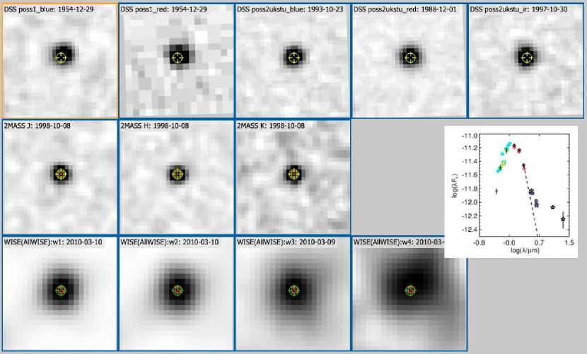
Figure 6: Reverse greyscale images of J052704.46+342559.0, obtained via FinderChart, in DSS (top row), 2MASS (middle row) and WISE (bottom row); images are 30$\arcsec$ across. The target position is given by the crosshairs; the additional colored symbols on top of that position are positions of corresponding catalog entries (the 2MASS and WISE catalog counterparts are exactly on top of this source). The inset is an SED using all the available data with symbols as defined in Table 2. Error bars are vertical black lines, most obvious here in WISE-4. Dashed line is the expected flux density from photosphere assuming $K_{\rm s}$ is on the photosphere. This source was identified by IPHAS as bright in H$\alpha$ and by Winston et al. (2020) as having an IR excess. This is a well-behaved point source, clearly and cleanly detected in the images, with a nice, YSO-like SED showing a clear IR excess; we accept this source as a high-quality YSO candidate.

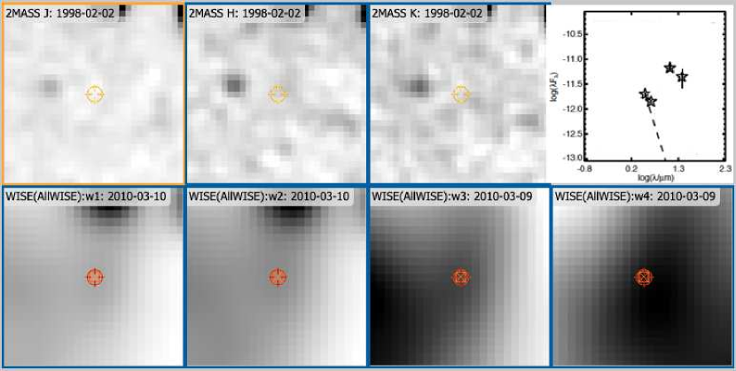
Figure 7: Reverse greyscale images of J052828.16+342411.7, obtained via FinderChart, in 2MASS (top row) and WISE (bottom row); images are 30$\arcsec$ across. The target position is given by the crosshairs. The top right is an SED using the existing photometric measurements for this source, four WISE bands (black stars); the dashed line is the expected photosphere if WISE-1 is on the photosphere. This source appears in the AllWISE point source catalog (red squares in the WISE images) as a high-quality detection; it also appears as a YSO candidate in Winston et al. (2020). However, as can be seen, there is no counterpart at 2MASS (or any other) bands, and the emission at 22 $\mu$m is significantly offset from the target position. The SED is inconsistent with that of a YSO. We dropped this source as likely to be a nebular knot, not a YSO.

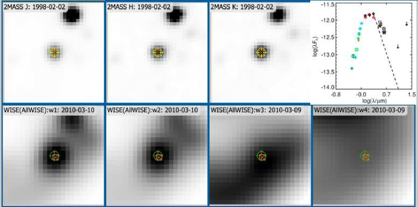
Figure 8: Reverse greyscale images of J052724.69+342049.1, obtained via FinderChart, in 2MASS (top row) and WISE (bottom row); images are 30$\arcsec$ across. The target position is given by the crosshairs, with an additional symbol for the corresponding catalog source. The top right is an SED with symbols as defined in Table 2. WISE-3 and 4 are both plotted here as limits. Dashed line is the expected flux density from photosphere assuming $K_{\rm s}$ is on the photosphere. This source appears in the AllWISE point source catalog with high-quality detections in all four WISE bands, but inspection of the image calls WISE-3 and -4 into question. The SED suggests that WISE-3 could be a detection and still be consistent with the rest of the SED; WISE-4 isn’t physically reasonable. We turned both the WISE-3 and WISE-4 detections into limits based on this image assessment. We retained this source as a YSO candidate; it was in the list of literature YSOs because it appears in Winston et al. (2020).

4.2 SED Inspection

After merging the available data (Sec. 2), we created SEDs for all the sources, combining all available data. The units of these plots (used in figures here, such as in Figs 6-8) are cgs units for the $\lambda F_{\lambda}$ axis, erg sec^-1 cm^-2, and the wavelength axis is in microns. Symbols used for the various data sets are listed in Table 2. Sample SEDs are provided here, but a full set of SEDs has been delivered to IRSA along with the data from this paper.

We have photometry ranging from 0.34 to 160 $\mu$m, but no stars have complete coverage over that whole range. The Koenig color selection requires at least the first three bands of WISE and 2MASS $H$ and $K_{\rm s}$, so all of the sources so selected must, by definition, have at least 5 points delineating their SEDs between 1 and 12 $\mu$m. For the worst-characterized sources (all in the regions of highest source surface density where source confusion is rampant, e.g., the heart of Stock 8 or in the NS), we may have only one or two points from Spitzer, or multiple detections but all at one or two bands (WISE-1 and -2 from AllWISE, CatWISE, & unWISE). Figure 9 has the distribution of points per SED. Nearly two-thirds of the sources have more than 20 points defining the SED, so for most sources, we have enough photometry to characterize the object fairly well. Just $\sim$10% have 5 or fewer points defining the SED. Later in the process (Sec. 4.4), objects that have fewer points in their SED are ranked as less confident YSO candidates. Most of the least-well-populated SEDs are in the NS, which is unsurprising given that we defined the NS by all objects encompassed by the polygon in Fig. 5, a region of high reddening and high source surface density (see more discussion below). Most of the best-populated SEDs are in Stock 8, which is the best-studied portion of this region (e.g., J17, Lata et al. 2019).

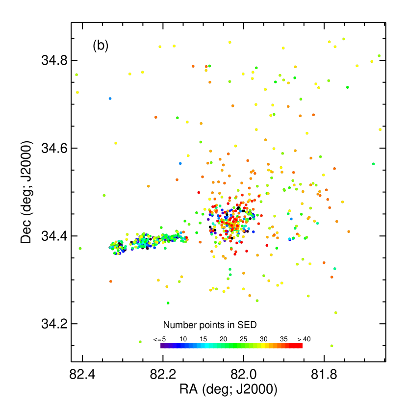
Figure 9: (a): Histogram of number of points in the SED created from the catalog merging. Nearly two-thirds of the sources have more than 20 points defining the SED, and just $\sim$10% have 5 or fewer points defining the SED. For most sources, we have enough photometry to characterize the object fairly well. (b): Distribution of points on the sky, where the color corresponds to number of points in the SED, where black=5 or fewer points per SED and red=35 or more points per SED (color scale shown in plot). Most of the best-populated SEDs are in the best-studied portion of this region, Stock 8. Most of the least-well-populated SEDs are in the NS, where SEDs can be only two IRAC points. (Compare to Figs. 2 & 5; see Sec. 6.1 for zoom-in on just the NS.) Given how many points we have in most of the SEDs here, we should be able to make some well-founded assessments of the status of most of these candidate YSOs.

We reviewed all the SEDs in conjunction with the image inspection (Sec. 4.1). We found sources likely to be nebular knots (Fig. 7). We identified cases where the position-based source matching across bands had clearly failed (Sec. 2.5), betrayed by an unphysically discontinuous SED; in those cases, we returned to image inspection and catalog merging, and checked to make sure the bandmerging across catalogs had been done correctly, finding and resolving any errors where possible. Some of the O and B stars are very bright, and unphysical SED shapes were a result not necessarily of source mismatch so much as saturation; in those cases, the counterpart at that saturated band was removed from the catalog. Some sources had [12] or [22] values that were unphysically discontinuous with the rest of the SED; we returned to the images and checked the AllSky (rather than AllWISE) catalogs to decide what measured flux value was most appropriate to use. In some cases where a point source was not apparent in the [12] or [22] images, we converted the values reported as detections in the AllWISE catalog for WISE-3 and/or WISE-4 into upper limits (see Fig. 8).

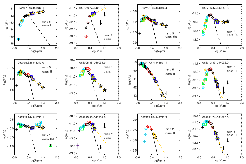
Figure 10: Twelve example SEDs, with plot symbols as defined in Table 2. The $y$-axis is the log of the spectral energy density in cgs units, e.g., ergs s^-1 cm^-2; the $x$-axis is the log of the wavelength in microns. The black dashed line is a Rayleigh-Jeans line extended from $K_{s}$, assuming that $K_{s}$ is on the photosphere of the star. The yellow dashed line is a fit to all available detections between 2 and 25 $\mu$m. The sources are, from top to bottom, left to right, are: J052807.89+341842.1, final rank 5, SED Class I; J052858.77+342232.5, final rank 4, SED Class I; J052718.35+344033.4, final rank 5, SED Class flat; J052736.37+344940.6, final rank 4, SED Class flat; J052705.83+343312.0, final rank 5, SED Class II; J052708.88+345031.5, final rank 5, SED Class II; J052717.77+342601.1, final rank 5, SED Class III; J052743.82+344028.0, final rank 4, SED Class III; J052919.14+341747.1, final rank 4*, SED Class flat; J052825.85+342309.6, final rank 4*, SED Class II; J052807.15+342732.3, final rank 2, SED Class II; and J052811.74+341625.0, final rank 3, SED Class III. See the text (and Appendix D) for more discussion.

Figure 10 provides twelve example SEDs, representing a range of YSOs. The reasons for their final rankings are discussed in more detail in Appendix D.

Despite some sources appearing point-like in the images, their SEDs do not look like textbook YSOs in that they could be more like quasars or nearby star-forming galaxies or even giants, but could also be consistent with highly variable YSOs. Follow-up spectroscopy will be required to determine the nature of these sources. We retained them as somewhat lower-confidence YSO candidates, largely on the basis of a Gaia distance that is in the right regime to be part of IC 417.

Following Wilking et al. (2001) and, e.g., Rebull (2015), we define the near- to mid-IR (2 to 25 $\mu$m) slope of the SED, $\alpha=d\log\lambda F_{\lambda}/d\log\lambda$, where $\alpha>0.3$ for a Class I, 0.3 to $-$0.3 for a flat-spectrum source, $-$0.3 to $-$1.6 for a Class II, and $<-$1.6 for a Class III. For each object, we performed a simple least squares linear fit to all available photometry (just detections, not including limits) as observed between 2 and 25 $\mu$m, inclusive. These classes are included in Table 4.

4.3 Color-Magnitude and Color-Color Diagrams

Koenig’s color selection cuts only use 2MASS and WISE, and selection of sources by position in the NS will only weakly constrain the YSO nature of the candidates. But we have considerable ancillary data (Sec. 2). We can therefore further cull sources by making color-color and color magnitude diagrams and investigating whether each source appears in positions consistent with a YSO status. This approach follows, e.g., Guieu et al. (2010) or Rebull et al. (2011).

Our process included identifying each star separately in several different color-color and color-magnitude diagrams; because we have so much available photometry, we have a lot of diagrams to choose from. The diagrams we used primarily included $J-H$ vs. $H-K_{s}$, [I1] vs. [I1]$-$[I2], [W3]$-$[W4] vs. [W1]$-$[W2], Pan-STARRS $z$ vs. $r-i$, Pan-STARRS $g-r$ vs. $i-z$, IPHAS $r-H\alpha$ vs. $r-i$, and Gaia DR3 $G$ vs. $G_{BP}-G_{RP}$ observed and absolute. Figure 11 shows four sample color-color and color-magnitude diagrams out of the several we used. In each case, points from the ensemble catalog are shown in addition to the YSO candidates. Reddening vectors as shown are calculated following the reddening law from Indebetouw et al. (2008) and Mathis (1990). The expected zero-age main sequence (ZAMS) in the near-IR is taken from Pecaut & Mamajek (2013), and the T Tauri locus as shown is from Meyer et al. (1997). The model isochrones in the PanSTARRS plot are 6 Myr and 9 Myr isochrones from PARSEC models (Bressan et al. 2012), shifted to 2 kpc. The IPHAS ZAMS is from Drew et al. (2005).

If a given object was an outlier in any diagram, we returned to its SED and even its images to determine if the data causing the outlying location was erroneous. For objects that appear as outliers, such as the apparently too blue sources in the IRAC color-magnitude diagram, checking the SEDs show that indeed there is something “off” for one or both IRAC channels for that object given the rest of its SED, but it is not severe enough, given the image and SED as a whole, to merit unhooking the star from the IRAC counterpart. Therefore, too blue in IRAC doesn’t exclude a source if the rest of the information we have about it suggests it is still a YSO candidate, but it may lessen the confidence we have that it is young and a member. We were able to notice patterns, such as the well-known feature that a faint measure in the Gaia blue band is often ‘off’ given the rest of the SED, so a Gaia $G$ vs. $G_{BP}-G_{RP}$ color-magnitude diagram presents many apparent faint outliers, whereas $G$ vs. $G-G_{RP}$ for those outliers may be fine. The faintest stars in PanSTARRS often have considerable scatter (unsurprisingly), which is readily apparent in both the SEDs and the color-magnitude diagrams. Sources that are outliers in more than one plot received more scrutiny and were demoted depending on the source’s properties.

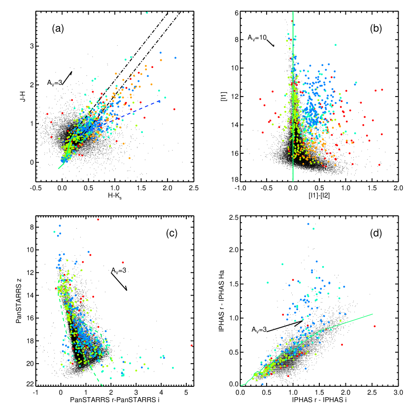
Figure 11: Sample color-color and color-magnitude diagrams used to assess further the quality of the YSO candidates. In each plot, small black dots are the ensemble catalog, and larger dots are the YSO candidates. Diagrams like this were used to assess the confidence we had that the YSO candidates were actually YSOs. Anticipating discussion in Sec. 4.4, the colors of the large dots follow the final YSO rankings. Targets ranked 5 (highest) are blue, 4 are cyan, 3 are green, 2 are orange, and 1 (lowest) are red; the bluer the symbol, the more reliable a YSO candidate it is. Many of the outliers are lower-ranked YSO candidates. The highest-ranked YSOs include both early-type stars and stars without too much $JHK_{s}$ reddening or a possible $JHK_{s}$ excess (a; upper left), stars with an IRAC excess (b; upper right), stars clustered near the 6 Myr model isochrone (c; lower left), and stars with an H$\alpha$ excess (d; lower right). Reddening vectors (following the reddening law from Indebetouw et al. 2008 and Mathis 1990) are as shown. Green solid lines are the expected (empirical) ZAMS relationship. In the $JHK_{s}$ plot, the ZAMS is taken from Pecaut & Mamajek (2013), the dashed blue line is the Meyer et al. (1997) T Tauri locus, and the dash-dot lines are reddening vectors extending roughly from the green ZAMS relation to give an indication of which of these stars could be reddened MS stars. The green dashed lines in the PanSTARRS plot are 6 Myr and 9 Myr isochrones from PARSEC models (Bressan et al. 2012). The IPHAS ZAMS is from Drew et al. (2005); the IPHAS data appear quantized due to the precision with which the magnitudes are reported in H$\alpha$.

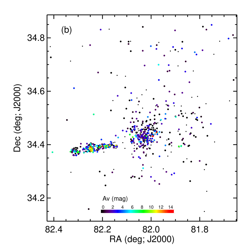
Figure 12: (a) Histogram of $A_{v}$ estimates, derived from $JHK_{s}$ as discussed in the text. The histogram peaks at $\sim$100 stars with $A_{v}\sim$0 (offscale here). The distribution falls off with $A_{v}$, with a max($A_{v}$) of $\sim$17 mag. (b) distribution of sources on the sky, with color corresponding to $A_{v}$ (redder point is more $A_{v}$). Small dots: sources for which we could not derive an $A_{v}$ estimate; larger circles are sources for which we could derive an estimate, and the redder the symbol, the higher the $A_{v}$ estimate. Most of the stars have little reddening. Most of the high-$A_{v}$ sources are in the NS, but the two with the highest estimate are in Stock 8 (compare to Figs. 2 & 5; see Sec. 6.1 for zoom-in on just the NS).

Because we are leveraging the position of each source in various color-color and color magnitude diagrams, reddening could be a significant factor in the placement of the star in said diagrams, particularly those using shorter wavelengths. To account for, estimate, and limit the influence of reddening, we wished to make plots where each star in question had been dereddened. In cases where we had $JHK_{s}$ for the target (93% of the YSO candidates), we were able to use the same dereddening approach as in Rebull et al. (2022; 2020) where we create a $J-H/H-K_{s}$ diagram and slide the observed $JHK_{s}$ back along a reddening vector (Indebetouw et al. 2005) to expected colors from Pecaut & Mamajek (2013) or the T Tauri locus (Meyer et al. 1997). This process results in merely an estimate of the reddening, but this is an efficient way to get an estimate. It fails outright for about a third of the targets, because, even given the best available $JHK_{s}$, there is no way to deredden and still end up in a reasonable location (see outliers in Fig. 11). As seen in Fig. 12, about 100 ($\sim$15%) of the stars end up with an estimate of $A_{v}\sim$0, and the distribution falls off steeply with $A_{v}$. There are more high-$A_{v}$ sources in the NS than any other place, but the largest estimates ($\sim$17 mag!) are for two very reddened (and embedded) stars in Stock 8.

For each target with an $A_{v}$ estimate, we plotted the color-color and color-magnitude diagrams with the observed and dereddened position indicated. In this fashion, we tried to distinguish (in optical diagrams) between reddened background giants and red YSOs, and included this consideration in the final ranking of the YSO candidates.

Additionally, for two diagrams, we explicitly calculated the significance of the excess, following, e.g., Mizusawa et al. (2012). For the IRAC data (e.g., Fig. 11), we calculated $\chi_{{\rm IRAC}}$, where

$$\chi_{{\rm IRAC}}=\frac{([I1]-[I2])_{\rm observed}-[I1]-[I2])_{\rm expected}}{\sqrt{\sigma_{[I1]}^{2}+\sigma_{[I2]}^{2}}}$$ (1)

For the mass ranges we are likely to detect in IC 417 (earlier than mid-M), $([I1]-[I2])_{\rm expected}$ is 0. We took there to be a significant excess in the IRAC bands when $\chi_{{\rm IRAC}}>$3; an IRAC excess suggests a dusty disk, making it more likely that a star is young. Similarly, for the IPHAS color-color diagram,

$$\chi_{{\rm IPHAS}}=\frac{(r-H\alpha)_{\rm observed}-(r-H\alpha)_{\rm expected}}{\sqrt{\sigma_{r}^{2}+\sigma_{H\alpha}^{2}}}$$ (2)

The expected $(r-H\alpha)$ is taken from the IPHAS ZAMS and is calculated assuming that $r-i$ is not subject to reddening, a poor assumption in general. However, the reddening vector is largely parallel to the ZAMS (see Fig. 11), so even large errors in reddening are unlikely to create a false H$\alpha$ excess. Here, again, we took there to be a significant H$\alpha$ excess when $\chi_{{\rm IPHAS}}>$3. An H$\alpha$ excess can arise from accretion in young stars, or from stellar activity. Stellar activity is generally higher in young stars (which are, on average, rotating faster than main sequence stars), so an H$\alpha$ excess can be indicative of youth. Because an H$\alpha$ excess need not uniquely identify youth, the influence of any H$\alpha$ excess on the final ranking of the star was less than the influence of any IRAC excess. Rarely, some stars appeared to have a $g$-band excess. The $\chi_{{\rm IRAC}}$ and $\chi_{{\rm IPHAS}}$ values, as well as an indication of whether or not stars had an IR excess, an H$\alpha$ excess, or a blue ($g$-band) excess, are all included in Table 4.

For those stars with measured Gaia DR3 parallaxes and distances from Bailer-Jones et al. (2021), we also looked to see if the star was between 1 and 3 kpc away (or had a distance that was within 1$\sigma$ of 1-3 kpc away), which is the expected range of distances we took to be associated with IC 417 (also see Appendix A on distances). We investigated whether or not proper motions would be helpful in selecting members of IC 417 (or for any of the clusters described in Sec. 1); there is nothing obviously helpful to be found among the proper motions, likely as a result of the significant distance.

4.4 Final Rankings

For each one of the sources that survived the vetting, we assessed whether or not the star, given all the information we had amassed, was consistent with being a YSO candidate. Each reviewer ranked the targets and then results were combined for a final net grade. We placed each in one of basically five bins, where 1 is less likely to be a YSO and 5 is more likely to be a YSO. We had to create additional major subdivisions in a few specific cases, discussed below. Within each of these ranks, we grouped apparently similar kinds of objects together, and then ordered them within each rank roughly by confidence, such that lower ordering within the rank was less confident. For example, in the lowest ranks, all of the YSOs that have only 2 IRAC points in their SED are grouped together, followed by those that have 2 IRAC and 1 2MASS point, then 2 IRAC, 1 2MASS, and 1 other point, and so on; in the higher ranks, stars with H$\alpha$ excesses as well as IR excesses can be found together, the OB stars can be found together, etc. The SEDs in the IRSA delivery are provided in this rank order so that paging through the SEDs is easy, and apparently similar objects can be found near each other in the list.

The rank 1 stars, based on the information we currently have, are least likely to be true YSOs at the distance of IC 417. There are several major subcategories within the rank 1 bin, which we now describe.

The “1r” (r for reject) stars are least likely to be young, consisting of stars that have to be rejected due to irreconcilable source confusion or because they are confirmed or likely carbon stars. There are three known carbon stars here, and we believe we have identified a fourth – see Sec. 7.

The next major category within the rank 1 bin is “1d” (d for distance), which means that the SED is well-defined, with many points, and it seems fine but has no obvious indications of youth, and moreover the Gaia DR3 distance is unambiguously too far or too close. With no good reason to retain it as young (besides the criterion/a that placed it in our YSO candidate list initially), we therefore put the star in the rank 1d bin.

The “1f” (f for few) means that the SED really has too few unique wavelengths to reliably assess it (typically $\lesssim$8-10 points). The 1f stars will need much more information before we can determine whether or not they are young and at the distance of IC 417. These stars could be young members of IC 417; we just don’t know yet.

The rest of the rank 1 stars are, in general, relatively unremarkable, relatively sparse SEDs (particularly by comparison to the rank 2-5 stars), with few indicators of youth or available distances. Rank 2 stars typically have more points in their SEDs than rank 1 stars, but still not a lot of indications of youth or available distances.

Ranks 3, 4, and 5 are where the most likely YSO members of IC 417 can be found. Typically, all of these stars have many points defining their SEDs. (Rank 3, 4, or 5 stars have on average $\sim$24 points in their SED, to be compared with $\sim$7 for rank 1 or 2.) In general, all the stars of rank 3 are sort of mid-grade in that there is no compelling reason to drop them (they are in places consistent with youth in all the relevant diagrams), but also no strong reason to keep them either, such as an excess of any sort, or even necessarily significant reddening. (Rank 3 stars have mean $A_{V}$$\sim$1 mag, and rank 4 or 5 stars have mean $A_{V}$$\sim$3-4 mag; see Fig. 11.) All the rank 4s and 5s have an excess of some sort – most commonly a significant IR excess, but H$\alpha$, and/or blue excesses can also be found (see Fig. 11). If there is a DR3 distance estimate for the rank 5s, it is in the right range, $\sim$1-3 kpc, to be a member of IC 417, at least within 1$\sigma$. If there are obvious and/or multiple signs of youth but the distance is not quite right, then the star is set as a rank 4. The subcategory “4*” is reserved for those that seem to have the right distance, and within a given survey, the colors seem ok (e.g., within PanSTARRS, the CMD placement is ok), but the complete, net SED shape is unusual or confusing, not necessarily suggestive of a YSO, and so follow-up spectroscopy is particularly needed to check on the status of these targets.

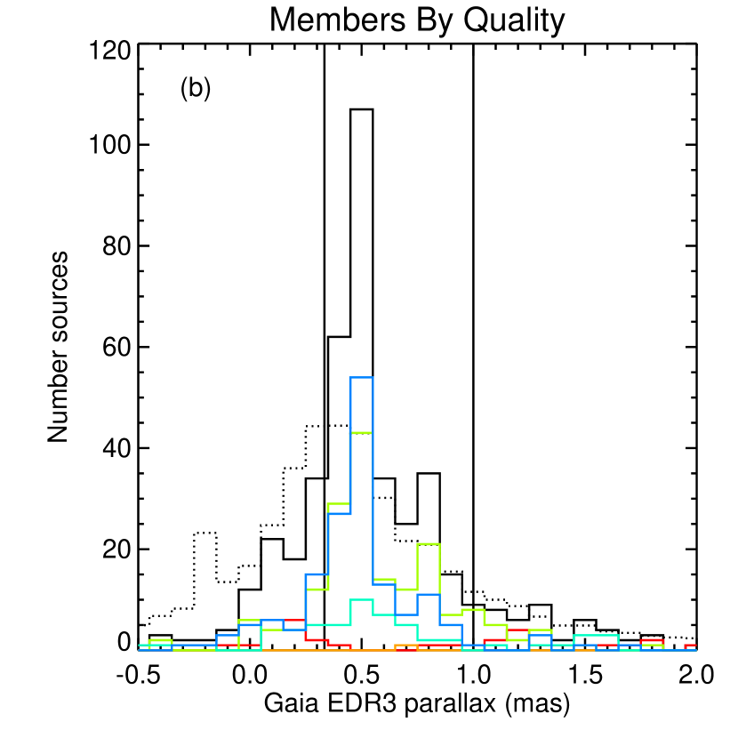
Figure 13: Histograms of Gaia DR3 parallaxes. (a): Solid line is all YSO candidates; dotted line is the rest of the catalog, scaled to have the same sample size as the YSO candidate sample. The solid vertical lines are at 1 and 3 kpc, e.g., the range of distances we took to be consistent with IC 417. The numbers on the right and left of the plot indicate how many objects in the member sample fall beyond the ranges of the plot (e.g., there are 13 stars with DR3 parallaxes $<-1$). The member sample is more tightly biased towards objects between 1 and 3 kpc; the rest of the catalog is slightly farther away, on average, consistent with it being largely the rest of the Perseus arm population. (b): zoom in on a smaller range of parallax, with the YSO rank plotted separately, color-coded as in earlier figures (5=blue or highest quality, 4=cyan, 3=green, 2=orange, 1=red or lowest rank). The bulk of the YSO candidates that are at the correct distance are largely rank 3, 4, or 5; the YSO candidates that are too close or too far away are largely rank 1 or 2.

Figure 13 shows a histogram of the parallaxes for the entire YSO sample, in context with a scaled histogram of parallaxes to everything in the catalog ($\sim$19,000). It also shows the breakdown of the parallaxes for each ranked sample of YSO candidates.

There is a strong peak among the YSO candidates at $\sim$2 kpc, which is approximately the expected distance of IC 417. We took 1-3 kpc as the range of distances we accepted as consistent with IC 417, and that range is indicated on the plot. The entire catalog is on average slightly farther away than IC 417, consistent with IC 417 being on the near side of the Perseus arm, as suggested by MN16. However, the peak of the background distribution is within the 1-3 kpc range we accepted as more likely to be members. This suggests that more work will be needed to identify objects securely as being part of IC 417. (Also see Appendix A on distances.)

The sources that are outside the 1-3 kpc range are more often lower-ranked YSO candidate quality, as a result of our selection approach. We accepted some YSO candidates as higher quality if the error bars on distance (as provided in Bailer-Jones et al. 2021) brought the star within range, and the SED/colors/excesses were consistent with youth, so some high-quality YSO candidates populate the bins outside the 1 and 3 kpc limits.

The rankings (the coarse rank and the ordering within each rank) are included in Table 4. The colors of the points in Fig. 11 reflect these 1-5 YSO rankings. For the remainder of the paper, the “entire YSO candidate sample” means the 710 that have made it this far. The highest-quality YSO sample is made up of the 503 stars that are ranked 5, 4, 4*, or 3.

5 The YSO Candidates

Figure 11 above shows several color-color and color-magnitude diagrams (also see Appendix C) with the points colored corresponding to final rankings. The $JHK_{s}$ and IRAC diagrams are the best-populated diagrams of all those that we constructed, because nearly all the sources (92%) have $JHK_{s}$ as well as both IRAC-1 and -2. The higher-ranked YSO candidates include the early-type stars, which can be seen distinctly in at least three of the four diagrams. Stars bright in IRAC with large IRAC excesses, as well as those with large H$\alpha$ excesses, tend to be highly ranked YSO candidates. Stars hugging the 6 Myr model isochrone also tend to be highly ranked YSO candidates. Stars that are likely FGK stars with little reddening, clustered around the ZAMS relation in the $JHK_{s}$ diagram, are typically rank 3, and they are also those stars that have no IRAC or H$\alpha$ excess, and appear roughly where expected, between the isochrones in the optical CMD. As described above, many of these rank 3 stars have nothing very obvious to reject or recommend them as YSO candidates, other than the property that placed them in the YSO candidate list initially. Many of the outliers in all the plots are lower-ranked YSO candidates. Many of the stars that appear to be likely giants in the optical CMD are rejected, as are many of the very red and faint stars in the IRAC CMD.

Figure 14 includes the same four color-color and color-magnitude diagrams as considered above, but now, among the rank 3-5 YSO candidates, highlighting those that have an H$\alpha$ excess, or a clear IR excess at any band. Most of the stars with an H$\alpha$ excess also have an IR excess, but as far as we can tell (given that our H$\alpha$ data does not cover our entire region), relatively few of the stars with an IR excess also have an H$\alpha$ excess, though we very well may be limited by data availability. On the whole, though, these points largely fall where we expect them to fall. Many IR excess sources are reddened in the $JHK_{s}$ diagram, with many having large enough IR excesses to influence the NIR. Most of these sources have significant IRAC excesses. Most cluster near the 6 Myr isochrone. Recall that our H$\alpha$ calculation (Sec. 4.3) made assumptions, but this diagram shows that our selection of H$\alpha$ excess stars is reasonably robust and hopefully indicative of youth.

We note that limiting this plot to the highest quality YSOs still includes several objects faint in PanSTARRS, resulting in large scatter. Looking at the SEDs for these stars, it is clear that PanSTARRS $r$ or $i$ is different than expected given the rest of the SED. Different optical color-magnitude diagrams show these stars in a more physically reasonable location. Additionally, some of the brightest stars highlighted in this diagram are suggestive of giants, and may in fact be older than YSOs; they persist here in rank 3 or 4 because they appear to have an IR excess, and we think they are more likely to be YSOs than giants based on the ensemble of data accumulated.

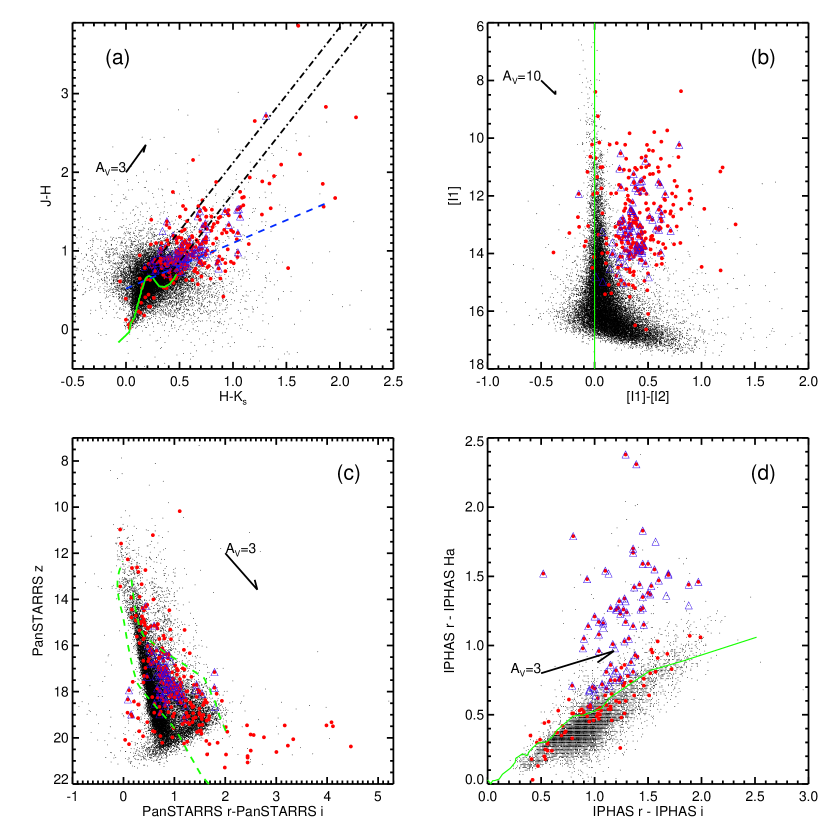
Figure 14: Color-color and color-magnitude diagrams as in prior figures; black dots are the entire catalog and colored symbols are limited to YSO candidates with rank 3-5. The stars highlighted with red dots are those with IR excess at any band (SED Class $<$ III plus Class IIIs that seem to have an excess at long wavelengths). Additional blue triangles are those with H$\alpha$ excess. Most YSO candidates with H$\alpha$ excess also have an IR excess, but relatively few of the IR excess stars have an H$\alpha$ excess. The stars with IR and/or H$\alpha$ excesses largely fall where expected in these diagrams – where YSOs are found (also see App. C).

Stars with very high accretion rates will not only have ultraviolet (UV) excesses, but may also produce a blue excess. Because we have $g$ from PanSTARRS, we explored whether selection of stars with an apparent blue excess would work for identifying YSO candidates. However, it does not work well in this sample for several reasons – there is a lot of scatter, especially at the short wavelengths where the stars are faint; there is a lot of uncertainty introduced by reddening; and these stars may not, on the whole, be young enough to have accretion rates sufficiently high as to make many large $g$-band excesses. We noted where $g$-band excesses happened to occur and used that information to bolster evidence for youth, but did not select new objects based on $g$-band excesses.

Figure 15 shows the distribution on the sky of the YSOs/candidates, color-coded by final rank. As noted earlier, (see Fig. 2 and 5), Stock 8 and the NS are both immediately obvious, because of the way our target list was constructed. High and low ranking YSO candidates are found throughout the region. The many low-ranking candidates in the NS and Stock 8 arise because these regions have such a high surface density of sources, and the NS has such high reddening, that many of the resultant SEDs are poorly sampled, and as a result are low ranking. This is a larger problem in the NS than Stock 8. Fig. 15 also plots the highest-quality candidates on the sky with colors corresponding to SED class. Most of the sources with very large IR excesses are also in the NS or Stock 8, though some are found throughout the field. (Of the 19 Class I sources that are rank 3-5, 11 are in the NS, and 4 are in Stock 8; of the 32 Flat Class sources that are rank 3-5, 10 are in the NS, and 8 are in Stock 8.) The majority of the sources in general, however, are Class III or II (see Table 3).

We note, however, that our sample is likely incomplete. Our Class III sample is least likely to be complete, given the generally IR-centric methods we (and those in the literature) have used to assemble our YSO candidate list. Our sample of YSO candidates not in Stock 8 or the NS is also probably less likely to be complete, because the wider field area has not been subject to as careful detailed scrutiny as Stock 8 or the NS.

Pandey et al. (2020) find fewer YSOs within one of the large bubbles that they identify, where IC 417 is on the southern edge of a bubble. Given that, we might expect to find fewer YSOs/candidates north of IC 417 than south of it. We do not see anything obvious consistent with that, but we may not be sampling a large enough area to adequately test this.

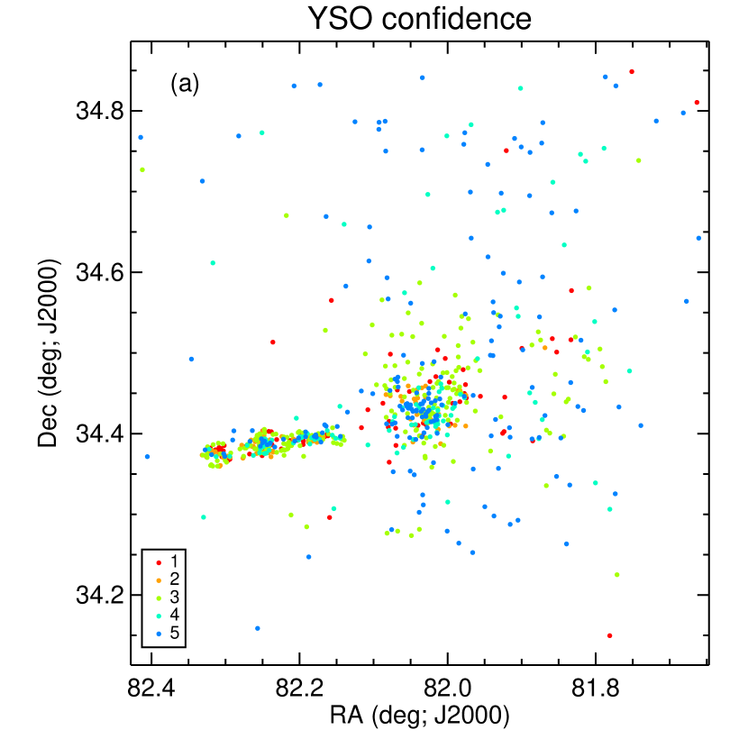
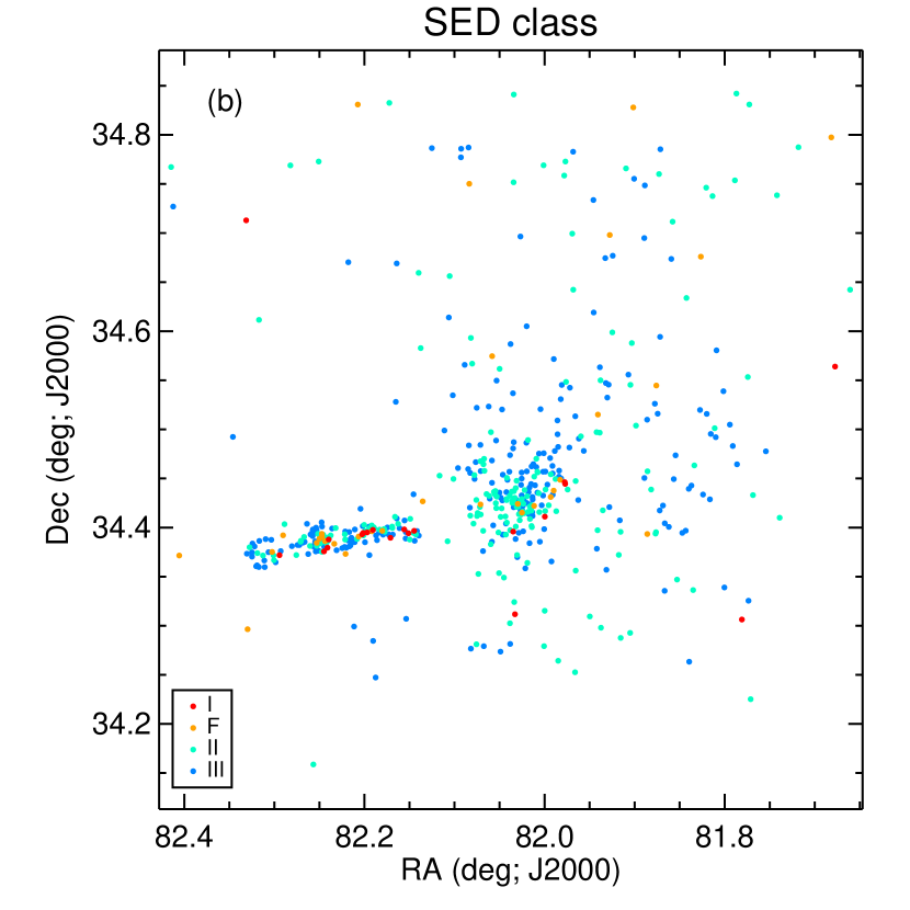
Figure 15: Distribution on the sky of YSO candidates. (In both cases, see Sec. 6.1 for zoom-in on just the NS.) (a): The YSO quality is color-coded as in earlier figures (5=blue or highest quality, 4=cyan, 3=green, 2=orange, 1=red or lowest quality). The clustering in Stock 8 and the NS is obvious by eye; this is a result of how we constructed our candidate list. Many of the lowest-ranked YSOs are in the highest surface density areas (NS and Stock 8) because they have the fewest points in their SEDs. (b): Just the rank 3/4/5s, and the SED slope is color coded (Class I=red, flat=orange, II=cyan, III=blue). Most of the embedded things are in the NS or Stock 8, but there are some scattered throughout the field. Most of the objects, however, are less embedded.

6 The Obvious Clusters

6.1 Stock 8 and the NS

In Figs. 1 and 2, Stock 8 and the NS are immediately obvious, Stock 8 because the cluster stands out against the background and the NS because of its nebulosity and red (or reddened) stars. In the distribution of YSO candidates (e.g., Fig. 5), Stock 8 and the NS are immediately apparent just because of how we picked the YSO candidates. In this section, we explore what, if anything, we can understand about the NS as a whole, comparing to Stock 8 (and to some extent the rest of the field).

J17 place Stock 8 at 3 Myr old, and the NS as younger still. Given the inventory of YSO candidates we have amassed, can we constrain these ages? One way we can do this is to assess disk fractions as a proxy for relative age. We can consider those that have a clear IR excess at any band – this includes objects with SED Class I, flat, or II, plus those of Class III whose SED has an unambiguous excess (either much smaller excesses than IIs, or emerging at longer wavelengths than can significantly influence the SED slope between 2 and 25 $\mu$m). The resultant overall disk fraction in the NS is $\sim$51%, in Stock 8 is $\sim$56%, and outside of either of those clusters is $\sim$56%. Assuming Poisson statistics, those numbers are identical, and it seems possible that all the stars here may indeed be on average about the same age. However, as noted above, it is likely, given our IR-centric methods of finding YSOs, that our Class III sample is incomplete, and perhaps we should work only with stars that have IR excesses. Considering the ratio of (Class I+Flat)/(Class I+Flat+Class II), the NS is 34$\pm$8%, Stock 8 is 12$\pm$4%, and the rest of the field is 21$\pm$6%. By this metric, then, the NS is the youngest, and Stock 8 is the oldest.

Figure 16 compares the NS to Stock 8 in color-color and color-magnitude diagrams. There are twice as many low-ranking YSO candidates in the NS as in Stock 8, but the distributions even without the low-ranking YSO candidates are distinctly different. There are 71 YSO candidates of rank 5 in Stock 8 (and 39 of 4/4*, and 93 of rank 3 for a total of 203) and just 24 YSO candidates of rank 5 (and 33 of 4/4*, and 79 of rank 3, for a total of 136) in the NS. There is more reddening and IR-excess-influenced NIR seen in the $JHK_{s}$ diagrams in the NS compared to Stock 8. Also based on the $JHK_{s}$ diagram, Stock 8 has more higher mass stars, but the uncertainties in reddening, particularly in the NS, may be limiting the number of higher-mass stars we can identify there based solely on photometry. There are more stars with larger IRAC excesses in the NS. The Stock 8 IRAC colors for the highest rank YSO candidates hover near [I1]$-$[I2]$\sim$0.5, whereas the highest rank YSO candidates in the NS are dispersed out to $\sim$1.5, though admittedly there are fewer of them. The optical color-magnitude diagram is the most uncertain in the NS because of the $A_{V}$ uncertainties, but there is less scatter in the Stock 8 distribution, which is constrained more tightly between the 6 and 9 Myr isochrones. The distance distribution is also markedly different perhaps due in part to reddening (there are about twice as many stars available in Stock 8 with Gaia distances than in the NS) – the histogram of distances to the few stars with distances in the NS is rather flat, and the distribution for Stock 8 is sharply peaked at $\sim$2 kpc. If the bin size is broadened for the less-well-populated NS, then there is a broad peak in the NS centered on 2 kpc.

It seems reasonably likely from our analysis here that the NS is younger than Stock 8, and both are at about the same distance. This agrees with some literature – J08 suggested that the NS is at about the same distance as Stock 8 (MN16 disagrees), and J17 found that the NS is likely younger than Stock 8.

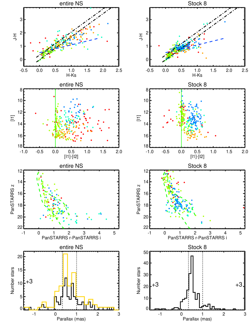
Figure 16: $JHK_{s}$ color-color diagrams (top row), the IRAC color-magnitude diagram (second row), and the PanSTARRS color-magnitude diagram (third row), and a histogram of parallaxes (fourth row) for the entire NS (left column), and Stock 8 (right column). Colors in the top three rows correspond to YSO ranks (as in Fig. 11 or Fig. 18), so bluer is better. Note that the limits of the $JHK_{s}$ plot are the same as earlier in the paper, but the limits are adjusted for the other two diagrams. The yellow line in the lower left histogram is with a broader bin size, because there are double the number of stars in Stock 8 (200) compared to the NS (92). The vertical dotted lines correspond to 1 and 3 kpc, the range of distances we took to be consistent with IC 417. The numbers at the left and right sides of the plot indicate how many outliers there are (e.g., there are 3 stars with parallax $<-1.5$ mas and 3 stars with parallax $>$3 mas in Stock 8). The NS is likely younger than Stock 8, and they are likely at the same distance.

6.2 Within the NS

The NS is one of the most striking things in Fig. 1, and the clumping of the red (or reddened) stars within it is immediately obvious. In Figure 5, we broke the NS distribution into those four sub-clusters just based on a by-eye assessment. NS 3 (defined there) is coincident with BPI 14, though the nominal definition of BPI 14 is larger than our NS 3. NS 3 is the best-populated sub-cluster in the NS, consistent with BPI 14 being obvious enough that it has been already identified as a cluster.

If there are differences across the NS, it would shed light on the star formation process happening here. The spacing of the clusters on the sky is one of the things that draws the eye. Measuring the cluster spacing by eye in a variety of ways and comparing the mean RA and dec for the stars defined for each cluster yields spacing of NS1 to NS2 of $\sim 90-100\arcsec$, NS2 to NS3 of $\sim 130-150\arcsec$, and NS3 to NS4 of $\sim 200\arcsec$. At 2 kpc, and assuming an isothermal sound speed of 0.3 km s^-1 (sound speed for dense hydrogen gas at 20 K), the sound crossing time for each clump is on the order of $\sim$200-400 Myr. If this is triggered star formation, and if the trigger is coming from Stock 8, we should be able to see a gradient across the chain, correlated with distance from Stock 8; if the trigger is coming instead from the north, as suggested by J08, then no age gradient will likely be apparent. Either way, however, there is no immediately obvious explanation for the semi-regular clumping of the clusters within the NS.

Because the sources in the NS are so close together, in all the plots above of the stars on the sky, it is hard to see what is happening in the NS. Figure 17 shows a zoom-in on the NS for several parameters discussed above for the entire sample. As a result of how we selected stars in the NS, many have very few points in their SED; some of the worst-sampled SEDs of the entire sample are in the NS. For those that have $JHK_{s}$, we can derive an $A_{V}$, from which we know that some of the most highly reddened sources in the sample are in the NS, specifically NS 2 and NS 3. There are objects with SED slopes suggesting very embedded sources throughout the NS, with the most embedded ones in NS 3. Distances are relatively rare in the NS, a result of the high $A_{V}$ and frequently embedded sources. Because there are so many poorly sampled SEDs, a direct result is that there are many low-ranking YSO candidates in the NS.

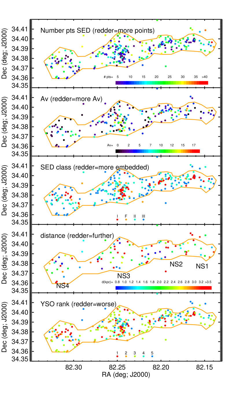
Figure 17: Zoom-in on the NS for several properties discussed earlier for the sample as a whole – number of points in the SED, amount of reddening ($A_{V}$) estimated from the $JHK_{s}$ diagram, SED Class (I/flat/II/III), distance from Gaia DR3 as derived by Bailer-Jones et al. (2021) (with additional annotations of the subclusters), and our final YSO confidence rank (1-5). Color scales are as indicated in each panel. Points are only plotted if there is a corresponding value – there are fewest points in the fourth panel because there are fewer distances known than anything else here. Because the YSO candidates in the NS were identified by position on the sky, many objects in the NS have very few points in their SED, which results in many low-ranked SEDs. There can be a lot of reddening (obvious in Fig. 1), which results in many sparsely populated SEDs, but also steep SEDs and few distances. NS3 has the most stars, the most $A_{V}$, and the most embedded sources.

Low-ranking YSOs can be found both too close and too far away (because the distance is incorporated into the source assessment) – for those $\sim$90 objects in the NS that do have DR3 distances, $\sim$40% have a distance from Bailer-Jones et al. (2021) that is $<$1000 or $>$3000 pc, e.g., nominally too close or too far away. However, the distance to IC 417 is not well known, and there are uncertainties on the stellar distances. Taking the errors provided by Bailer-Jones et al., just 15% of the NS objects with distances are unambiguously too close or too far away – for example, their distance is $>$3 kpc and their lower limit on distance is also $>$3 kpc.

Figure 18 shows the $JHK_{s}$ color-color diagram, the IRAC color-magnitude diagram, and the PanSTARRS color-magnitude diagram for various parts of the NS. Note that these are three of the same diagrams shown earlier and are using the same notation as Fig. 11, but the axes in the IRAC and PanSTARRS are optimized for this sample. There are no obvious differences across these clusters in these diagrams, having tried various tests including a 2D Kolmogorov-Smirnov (KS) test, including for subsets of the data (e.g., just ranks 3/4/4*/5 for each box in Fig. 18). It is likely that either they are all about the same age (and mass, and reddening, and IR excess) distribution, or the uncertainties in age are comparable to the age spread, or that small number statistics are masking any differences.

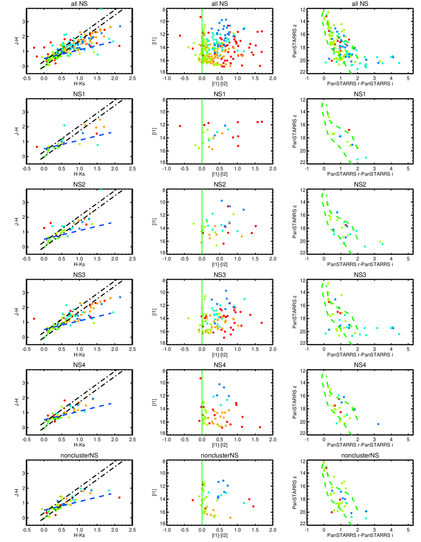
Figure 18: $JHK_{s}$ color-color diagrams (left column), the IRAC color-magnitude diagram (center column), and the PanSTARRS color-magnitude diagram (right column) for various parts of the NS: the entire NS (first row), just NS1 (second row), just NS2 (third row), just NS3 (fourth row), just NS4 (fifth row), and those NS stars not assigned to a subcluster (sixth row). Colors correspond to YSO ranks (as in Fig. 11), so bluer is better. Note that the limits of the $JHK_{s}$ plot are the same as earlier in the paper, but the limits are adjusted for the other two diagrams. There are no obvious differences among the clusters, other than NS 3 being the best-populated.

The overall disk fraction is a function of how one defines the disk fraction. In terms of all YSOs, IR excesses at any band, the overall disk fraction in the NS is 64$\pm$6% (assuming Poisson statistics). However, we can take only the high quality YSOs (3/4/4*/5) and any IR excess and get 51$\pm$8%. Further, taking only the high quality YSOs (3/4/4*/5) and only large IR excesses (SED Classes I and flat), the overall fraction is 16$\pm$4%. Looking across the NS, among each of the 4 clusters and the non-cluster NS stars, and assuming Poisson statistics, in each case, comparable disk fractions are obtained. So there is no discernible difference across the NS when considering disk fraction. Again, all evidence seems to suggest that they are all about the same age.

We conclude that it is indeed most likely that any star formation trigger is coming from the north, not from Stock 8, as suggested by J08.

As noted above, Dewangan et al. (2018) concluded that most of the star formation was happening in what they termed ns1, and none in ns2. We did not select any stars from the region consistent with their ns2, because there were not any clumps of red stars in Fig. 1, and we agree that their ns2 is far more “boring” than their ns1 (our NS). Dewangan et al. estimate that there are $\sim$80 YSOs forming here. We started with $\sim$260 YSO candidates in the NS; in the end, we have 24 that are rank 5, 33 that are rank 4 or 4*, 79 that are rank 3, 56 that are rank 2, and 65 that are any kind of rank 1. Taking all the rank 3/4/4*/5 YSO candidates, that is 136, which is about 70% more than Dewangan et al. estimated. Additional work will be required to estimate a total mass in YSOs.

J08 find that the NS is likely excited by an O8 star from the north, and that the ionization front from Stock 8 has not yet reached the NS. They also find that the stars in what we have called NS3 are likely younger than Stock 8. Our findings are consistent with this. MN16 further identify BD+34$\arcdeg$1058 as the ionizing source for the NS; this is one of the stars featured in the next section.

7 Specific Stars of Interest

There are 32 known OB stars in this region and three known carbon stars. As part of our analysis here, we believe we have identified one new carbon star. The OB stars are young and the carbon stars are old, but all are bright.

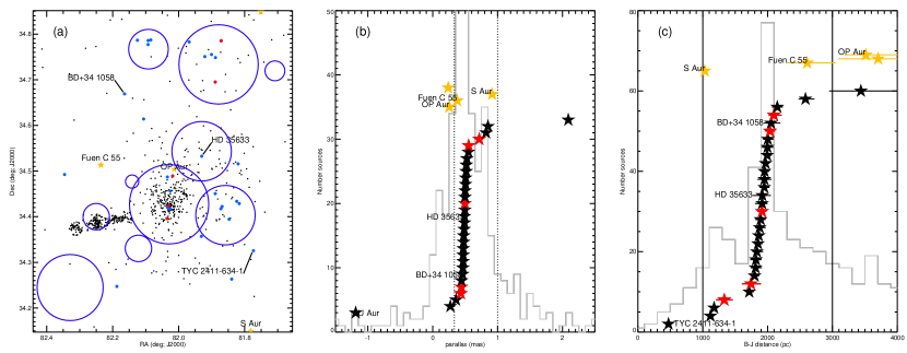
Figure 19: (a): Plot on the sky of the YSO candidates (small black dots), with the cluster circles from Fig. 5 (blue circles; unlabeled here just for clarity). The OB stars are highlighted (larger blue dots); those OB stars with apparent IR excesses are larger red dots. In all plots, three OB stars are highlighted. HD 35633 is thought to be the powering source for the nebulosity around Stock 8 (MN16). BD+34$\arcdeg$1058 is thought to be the driving source for the NS (MN16). TYC 2411-634-1 is too close to be a member of IC 417. The four carbon stars are also indicated by the yellow stars in both plots; known carbon stars have their names indicated, and the unlabeled gold point is the newly identified carbon star. (b) and (c): Histograms of parallaxes and distances to the final set of YSOs in grey, with the locations of the OB and carbon stars highlighted at arbitrary $y$-axis positions as 5-pointed stars (with the uncertainties from Bailer-Jones et al. 2021 indicated by horizontal lines). Red symbols are stars with disks. The carbon stars are indicated in yellow. Certain stars are called out. One has a parallax so negative as to not appear in panel b (J052729.32+342502.6=[JPO2008] IC 417 3); and that one, plus one more (J052752.39+344658.1=IU Aur), have distances too far to appear in panel c. The OB stars are distributed across the sky and in distance, but may preferentially appear in the clusters. They are certainly clustered at the distance of IC 417 (1-3 kpc). The carbon stars are not young and are unlikely to be members of IC 417.

Figure 19 shows the location of the OB and C stars on the sky. Figure 19 also includes the parallaxes and distances to the stars, which are available for all the OB and C stars. A few of the published parallaxes are negative, which is why we have also plotted the distances from Bailer-Jones et al. (2021). Several things are of note in this figure.

Most of the OB stars are (in projection) within the literature clusters from Fig. 5; just 8 of them are not within the clusters. There are some clusters without known OB stars, however; there are no OB stars known in the NS. HD 35633 is called out in the Figure because it is thought to be the powering source for the nebulosity around Stock 8 (MN16); similarly, BD+34$\arcdeg$1058 is thought to be the driving source for the NS (MN16).

Most of the O and B stars are at the correct distance to be members of IC 417. The two stars that MN16 proposes as powering the NS and Stock 8 are both within 2-3 kpc.

One nominal OB star, J052740.98+344502.5=TYC 2411-634-1, at $\sim$470 pc, is too close to be a member of IC 417. Ness et al. (2016) identifies it as a red giant, which is quite inconsistent with the B8V type listed for it in MN16. The object’s optical colors could be consistent with a giant, but given the distance, it is not very far above a 6 Myr isochrone, and does not seem to be subject to very much reddening. It is unclear what is going on with this source.

Two other OB stars (J052729.32+342502.6=[JPO2008] IC 417 3, and J052752.39+344658.1=IU Aur), appear to have distances in excess of 6 kpc, too far to be members of IC 417.

Neither one of the stars powering the NS or Stock 8’s nebulosity appears to have an IR excess, but there are 5 other OB stars that appear to have IR excesses, three of which are in Stock 8, and two of which are in FSR 777, and all of which are at the right distance to be part of IC 417. Because the long wavelength surveys we have are relatively poor resolution, if there is a nearby (in projection) cooler star to the OB star in question, or surrounding nebulosity, it can manifest as a long-wavelength IR excess in the SED. A lower-mass binary companion could also result in a small IR excess.

We collect a few notes on specific OB IR excess sources here. The sources J052729.13+344707.2 (LS V +34 17) and J052733.43+344141.6 (LS V +34 20) are both in FSR 777. The available spectral types in the literature are B2V (MN16) or B2III (Chargeishsvili 1988), and B1.5V (MN16) or B0III (Chargeishsvili 1988), respectively. They both appear to only have an excess at 22 $\mu$m. There are nearby red sources, but in both cases, the possible polluting source is far enough away that WISE can resolve the target. The remaining sources are all within Stock 8, where the source surface density is high, but the images seem clean enough that we retained these sources. Source J052804.41+342921.0 (LS V +34 27) is relatively isolated and has a clear IR excess at 12 and 22 $\mu$m; it is a B2IV (MN16). Source J052807.13+342526.8 (BD+34 1054) is an O9.7IV (MN16) or B0V (Chargeishsvili 1988), and it has an IR excess measured by both WISE and MSX. The SED suggests, however, that the detections at 7.7 $\mu$m and longer might be contaminated by nebular emission. The images indicate that the photometry is relatively uncontaminated. Finally, source J052808.37+342345.2 (BD+34 1056) is a B0.5V (MN16) or a B0I (Chargeishsvili 1988). It has an IR excess measured by both WISE and AKARI. Like the previous source, the SED might be contaminated by nebulosity, but the images look good. Further assessment of the origin and reliability of the IR excess in these sources will require additional data, beyond the scope of this work.

The carbon stars are not young, but have an unambiguous IR excess in their SEDs – their SEDs are well-populated and have an IR excess at multiple bands from multiple instruments. There are three known carbon stars here – J052707.44+340858.6=S Aur, Nassau & Blanco (1954), a C-N5+ according to Barnbaum et al. (1996); J052803.23+343013.8=OP Aur, a C0-C1e according to Kohoutek & Wehmeyer (1997); and J052856.65+343048.1=Fuen C 55, a C D according to Fuenmayor (1981). We identified one new likely carbon star here, J052700.29+345055.0. It was brought to our attention initially because it was identified as variable in ASAS-SN. S Aur is too bright to have data from the Zwicky Transient Facility (ZTF; Bellm et al. 2019), but the other three have $i$ and $r$ light curves suggestive of carbon stars. (Detailed discussion of the ZTF light curves of the entire IC 417 sample is beyond the scope of the present paper.) Looking at the SED, placement in CMDs and color-color diagrams, and even its variability properties (in ASAS-SN and ZTF), we strongly suspect that it is also a carbon star; follow-up spectroscopy is warranted. (This new candidate carbon star is in the 1r bin with the other known carbon stars.) OP Aur is apparently in projection within Stock 8; Fuen C 55 is close to it in declination but not within a cluster. S Aur is barely in the field under consideration in this work, on the south side. The star we believe to be a newly identified carbon star (J052700.29+345055.0) is also barely in the field, but this time on the north side. Two of the C stars have Bailer-Jones et al. distances between 1-3 kpc; the other two are a bit further away.

Because the carbon stars are nearing the ends of their lives, they are not expected, necessarily, to be clustered with any ostensibly young star clusters that may (or may not) be making up the constituents of IC 417. However, the OB stars are young, and cannot have moved far from their formation site, and thus are expected to be clustered. Several clusters (beyond Stock 8 and the NS) are identified in the literature here (Fig. 2), and most of the OB stars appear, in projection at least, to be coincident with these clusters (Fig. 19). In the next section, we consider whether or not we can distinguish these clusters from the rest of our sample.

8 The 2MASS Clusters

Table 5: Some Information on the Literature Clusters from our Catalog

Name	# YSO candidates (all)	# YSO candidates (3/4/4*/5)	# srcs in catalog	srcs/sq.asec
CBB 7	0	0	189	0.0074
FSR 777	22	21	3891	0.0096
FSR 780	35	31	2061	0.0090
CBB 3	34	31	1602	0.0070
Kronberger 1	6	6	1210	0.0119
CBB 4	0	0	258	0.0057
CBB 5	0	0	57	0.0050
CBB 6	1	1	2464	0.0087
Stock 8	279	208	4220	0.0104
BPI 14	125	66	275	0.0061

Much of the early analysis done in the IC 417 region used 2MASS star counts to identify several clusters (see Sec. 1 and Fig. 2). If they are really $\lesssim$10 Myr, as claimed, then there should be plenty of young stars in them waiting to be found. However, in Fig. 15, which does not have the cluster circles overlaid, one would be hard-pressed to identify the locations of the clusters besides Stock 8 and the NS (which includes BPI 14), hereafter referred to as ‘the 2MASS clusters’; they do not obviously stand out against the background when just the YSO candidates are plotted on the sky. However, it is true (Fig. 19) that most of the OB stars are coincident with the 2MASS clusters.

The literature did not publish detailed lists of candidate members of these 2MASS clusters; the analyses were based on statistics and star counts, and the clusters were defined via a circle’s position and radius on the sky, and so this is what we have done as well. This approach does not result in enough YSOs or candidate YSOs per cluster from our final list to do much analysis; Table 5 collects information about the clusters as they appear in our catalog, including the numbers of stars from our YSO candidate catalog. Aside from Stock 8 and BPI 14 (in the NS), there just are not very many stars in most of the 2MASS clusters. That could be because the clusters are of different sizes on the sky, or a result of our selection process. Our selection process is IR-biased, in that a reasonable fraction of our YSO candidates were identified via IR excesses, and our catalog is biased towards IR catalogs. However, the process for identifying these clusters in the first place is based on 2MASS star counts, so is also IR-biased. If we cannot find obvious evidence for the clusters in our YSO catalog, it is worth looking in our larger catalog. Table 5 notes the total numbers of sources (likely overwhelmingly stars) in our catalog in each cluster, even though it is incomplete and/or biased; since the clusters are different sizes on the sky, the number of sources (in projection) per square arcsecond is also noted. Among the 2MASS clusters, FSR 777 has the most sources, but Kronberger 1 has the highest surface density of sources, comparable to Stock 8.

We tested several different parameters and parameter combinations, including $K_{\rm s}$ histograms, distance histograms, color-color and color-magnitude diagrams such as those earlier in this paper. (Gaia proper motions here may shed additional light eventually, but are not any material help at this time.) For the most part, these diagrams reveal what we already know – Stock 8 and BPI 14 are different than the rest of the clusters, with BPI 14 being most obviously apparently younger. Even without clean membership lists, it is clear that these clusters are not the same age as Stock 8 and BPI 14.

Another approach we can take is to compare circles of the same size as these clusters placed randomly in the field, and compare color-color and color-magnitude diagrams to see if the diagrams from the purported clusters are different than those randomly placed. For each of the 2MASS clusters, we randomly dropped between 200 and 300 pseudo-cluster circles of the same size elsewhere in the field, making sure not to overlap with the NS or Stock 8. We compared $J$ vs. $H-K_{\rm s}$, $z$ vs. $r-i$ (from PanSTARRS), and [i1] vs. [i1]$-$[i2] for stars in each pseudo-cluster with the true cluster using a 2-dimensional 2-sided Kolmogorov-Smirnov (KS2d2s) test, and looked at the distribution of probabilities that resulted. We also did this for Stock 8 and BPI 14 as a ‘control’ of sorts; both of those clusters were obviously different than the field for every test we implemented. For CBB 4, CBB 5, CBB 6, and CBB 7, the results of our tests suggested these clusters were indistinguishable from the field. For Kronberger 1, it was less obvious that the results were different than the field, so we experimented with smaller cluster radii, since an overdensity of point sources can be seen in this area in the IRAC and WISE images. These experiments did not result in more clarity. CBB 3 seemed to be different than the field in PanSTARRS $z$ vs. $r-i$ but perhaps not in the two IR CMDs. FSR 777 and FSR 780 were both significantly different than the randomly placed field circles. More work is needed to assess whether or not these clusters are real and, if so, extract their members from the background.

We conclude that the additional clusters identified here from 2MASS star counts are evidently not $\lesssim$10 Myr; they are not the same age as Stock 8 and the NS or BPI 14. The 2MASS clusters, as far as we can tell, are older than Stock 8, if they are real. They may or may not be legitimate clusters; FSR 777 and FSR 780 seem to stand the best chance of being legitimate clusters, in that they seem significantly different than randomly selected fields in the vicinity.

9 Summary

IC 417 is in the Galactic plane, about 2 kpc away, with at least portions of it thought to be young, $\lesssim$10 Myr. We started by assembling YSO candidates from the literature, consisting of O and B stars, H$\alpha$-bright stars, IR excess stars, and variable stars. We defined a polygon on the sky encompassing the nebulosity and red point sources seen in Fig. 1, and identified all of the sources in the catalog within that polygon as potential new YSO candidates in the Nebulous Stream (NS). We identified new YSO candidates using IR excesses identified using WISE+2MASS data. We then vetted each of these YSO candidates by inspecting images where possible, constructing and inspecting SEDs, and constructing and inspecting various color-color and color-magnitude diagrams. There are 710 YSOs or YSO candidates that made it through this process, nearly two-thirds of which have more than 20 points defining their SEDs. We placed those 710 YSOs or candidates into ranked bins, from which 503 were in the higher (more confident) rank 3-5 bins. Of those 503, half are SED Class III, and $\sim$40% are SED Class II. The lowest ranking bins (1 and 2) include stars less likely to be YSOs; some of the stars in bin 1 include stars that are irreconcilably subject to source confusion or likely carbon stars.

We rediscover three literature carbon stars (S Aur, OP Aur, Fuen C 55), and identify one new candidate carbon star (J052700.29+345055.0). These objects are retained in the YSO candidate list in the lowest ranked bin, subgroup 1r (“r” for reject).

Follow-up spectroscopy will be necessary to confirm or refute the young-star status of the YSO candidates (and the new carbon star candidate) presented here. The variability properties of these stars may also help constrain their young-star status.

Because of the way in which we constructed our YSO candidate list, two clusters are very obvious in the YSO candidate distribution. Stock 8, which is well-studied in the literature, is well-represented in the YSO catalog. We identified all stars within the NS as candidate YSOs, so that region is also immediately apparent in the YSO catalog. (BPI 14, a literature-identified cluster, is the most densely populated part of the NS.) Our results agree with some of the literature (J08, J17) in that we find that the NS and Stock 8 (and the rest of the YSO candidates for which we have distances) are at about the same distance, $\sim$2 kpc, and the NS is the youngest region, with Stock 8 a little older. We do not find any evidence for an age spread within the NS, consistent with the idea that the trigger for the star formation event came from the north (J08), but our information may be limited by reddening and small-number statistics. We do not find that the other literature-identified 2MASS clusters here are as young as either the NS or Stock 8; at best they are older than Stock 8. They may not all even be legitimate clusters. There are some literature-identified OB stars that are coincident with some of those literature-identified clusters, however.

Spitzer, 2MASS, IRSA, WISE, Simbad, Vizier

Appendix A On the Distance to IC 417

As discussed above, there have been a variety of distances determined to IC 417: 2.97 kpc (Mayer & Macak 1971); 2.3 $\pm$0.7 kpc (Fich & Blitz 1984); 1.897 kpc (Malysheva 1990); 2.68 kpc (Mel’Nik & Efremov 1995); 2.05$\pm$0.1 kpc (J08); 2.7 kpc (Camargo et al. 2012); 2.80${}^{+0.27}_{-0.24}$ kpc (MN16); and 2.8 kpc (Dewangan et al. 2018). We adopted a distance of $\sim$2 kpc, and accepted as likely members anything between 1 and 3 kpc. We did not set out to determine a distance to IC 417, and moreover, we did not impose a tight constraint on the distances for each candidate YSO; if the 1$\sigma$ errors on the distance brought the star within 1-3 kpc, we allowed the star to remain a candidate YSO. In this Appendix, we briefly summarize why we made this decision.

There are many different available distance estimates based on Gaia data, and evaluating the details of all of them is beyond the scope of this paper. As noted above, some parallaxes in DR2 and DR3 are negative, leading us at least initially to turn to Bailer-Jones et al. (2018, 2021) for distance estimates. In Bailer-Jones et al. (2021), two distances are provided, geometric and photogeometric. In DR3 itself, a distance is provided from the General Stellar Parameterizer from Photometry (“GSP-Phot”; Andrae et al. 2022). All of these methods have limitations, particularly when the fractional uncertainty in the parallax is large, and they may not do well much past 2 kpc in general.

Figure 20 shows the distribution of all of the available distances for all of the (presumed) stars in our catalog. Given these raw distributions, it is clear that we are operating near the outer range of where these distances are largely available, let alone where they may be valid. Most of the available distances peak within 2-3 kpc; the DR3 Bailer-Jones geometric distances peak just past 3 kpc, but according to Bailer-Jones et al. (2021), these may not be the best distances to use for our situation, where the fractional uncertainties in parallax may be large. The DR3 GSP-Phot distances are apparently the most inappropriate for us to use, as they are most biased towards $<$1 kpc, even when dropping all the parallaxes with the largest uncertainties.

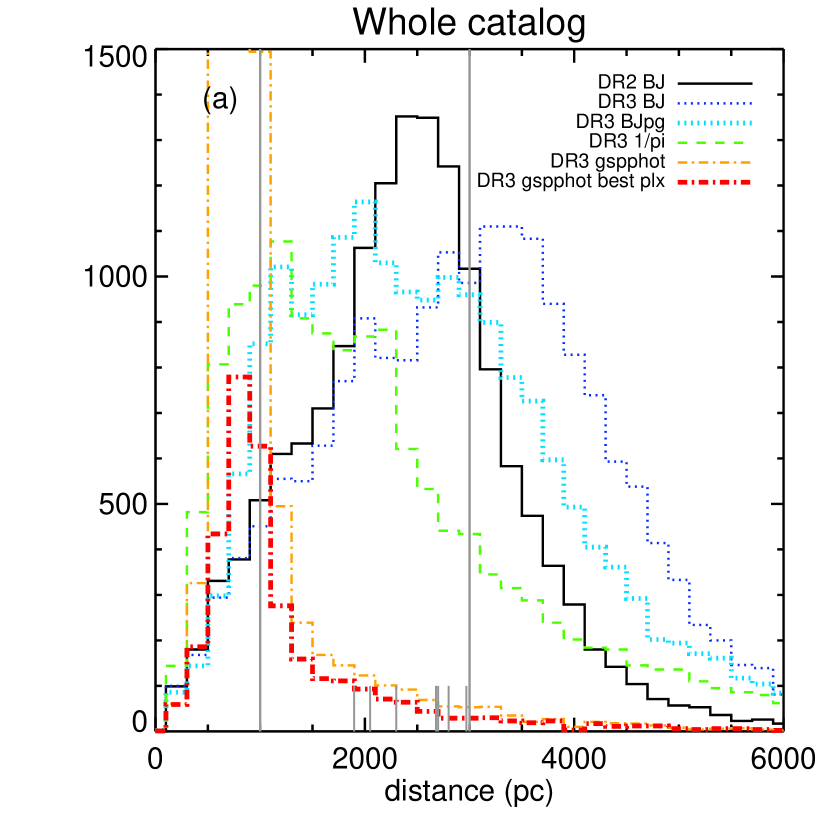
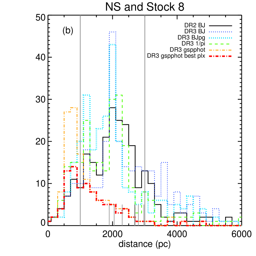
Figure 20: Histograms of distances from the (a) entire catalog in this region, and (b) just the NS and Stock 8. Legend in the upper right, e.g.: solid black line (DR2 BJ) = DR2 Bailer-Jones et al. (2018) distances; dotted thin dark blue line (DR3 BJ) = DR3 Bailer-Jones et al. (2021) geometric distances; dotted thick turquoise line (DR3 BJpg) = DR3 Bailer-Jones et al. (2021) photogeometric distances; dashed thin green line (DR3 1/pi) = distance from inverted parallax from DR3; dash-dot thin orange line (DR3 gspphot) = distance from GSP-Phot from DR3 (note that the peak is up well beyond the top of the plot, at 2345); dash-dot thick red line (DR3 gsppphot best plx) = distance from GSP-Phot from DR3 but only for those stars where the error in parallax/parallax $<$0.2 (e.g., those where Andrae et al. 2022 say the distances are likely valid). The grey vertical lines going from the top to the bottom of the plot are at 1 and 3 kpc, e.g., the range of distances we accepted as members of IC 417. The short, thick grey lines at the bottom are the literature distances given for IC 417 summarized in the text. Given these bulk distributions on the left, it is clear that we are operating near the outer range of where these distances are available, let alone where they may be valid. The distributions on the right show that the distances of stars in the NS and Stock 8 are peaked at 2 kpc, which is the main reason that we took stars with a distance of 2 kpc, with a range of 1-3 kpc, as members of IC 417.

Stock 8 and the NS are the best-populated clusters in IC 417. Figure 20 also has a histogram of just the distances to stars in those clusters. Ignoring the DR3 GSP-Phot distances, now all of the remaining distance distributions peak at 2 kpc. This is the main reason that we took stars with a distance of 2 kpc, with a range of 1-3 kpc, as members of IC 417.

Note that the literature distance values are primarily slightly farther than 2 kpc. A more secure (and less circular) distance determination will require work beyond the scope of this paper, including spectroscopy. Later Gaia data releases may also shed light on this subject.

Appendix B On Source Matching and Correcting Coordinates

Sec. 2.2 mentions that we had to correct the coordinates provided in J08 and J17 to match those in 2MASS before we could sensibly and accurately match them to the rest of the catalog. A few more details on this process are provided here. In Rebull (2015), a similar goal was to reconcile coordinates of YSOs from NGC 1333 over 20 years of literature. Here in IC 417, there is less of a time baseline, but similar fundamental issues of errors in the warp and weft of the world coordinate system (WCS) as applied to observations of small regions, resulting in distortions of the derived coordinates for any given source. We took the experience gained from Rebull (2015) and other similar work and applied it here.

The IRSA Firefly-based tools (called IRSA Viewer, Finder Chart, and the Catalog Search Tool, among others) provide interactive ways to overlay catalogs on images, and easy access to 2MASS images and catalogs, where those coordinates are robustly tied to J2000 (Skrutskie et al. 2006), and to Spitzer data and catalogs (both 2MASS and Spitzer are registered to the same coordinate system; IRAC Instrument and Instrument Support Teams 2021). The IRSA Firefly-based tools provide ways to click on sources and have the images zoom to center the source in question, the catalogs highlight the source in question, and the plots highlight the source in question. They can make plots, e.g., of position on the sky or attempt to make matches by position and plot offsets in position.

By overlaying catalogs from any given literature (such as, but not limited to, J08 or J17) on 2MASS images and trying to match these source catalogs to the 2MASS catalogs, one can easily identify pattern offsets. For example, it becomes obvious that in one portion of the sky, all the sources from a given literature catalog are offset from the sources in the 2MASS image by 0.73$\arcsec$ with a position angle of 30$\arcdeg$, but in another portion of the same catalog, the sources are offset from those in 2MASS by 1.58$\arcsec$ with a position angle of 102$\arcdeg$, or that in this strip of sky which must be an overlap region between two tiles in the observations that generated the catalog, there are two copies of every source in the catalog where one of each pair is offset by 1.3$\arcsec$ in the same direction from the other of each pair.

For the present work, specifically for J08 and J17, we did automatic position matching between those catalogs and 2MASS where possible, but in both cases, we discovered large, systematic, location-dependent offsets and frequent duplicates within the catalogs. We took care of these matches by hand using IRSA tools to overlay catalogs, identify sources, solve duplicate issues, and make matches between catalogs where necessary. If a match could not be found with 2MASS, it was checked against Spitzer in case the counterpart was too faint for 2MASS but appeared in Spitzer. The fact that the resultant SEDs make sense (e.g., that the J08 and/or J17 points are consistent with the rest of the points in the SED) is assurance that we have made the match correctly.

Appendix C Background Information on YSOs

This section provides an explicit discussion of each of the color-color and color-magnitude diagrams that we most frequently used, including a demonstration of where young stars and background objects are expected to be found. Since this kind of material was developed as part of the NITARP learning process for the high school teachers and students involved in this project, we have included a summary of this here in the hopes that other learners can benefit.

C.1 Definitions

A magnitude is really a flux ratio, defined as:

$$M_{1}-M_{2}=2.5\log\frac{F_{2}}{F_{1}}$$ (C1)

The magnitude system is traditionally defined to be referenced to Vega; that is, Vega is defined to be zero magnitude, and magnitudes of everything implicitly reference that flux:

$$M=2.5\log\frac{F_{\rm Vega}}{F}$$ (C2)

We note for completeness that calibration in the IR is complicated because Vega has an IR excess, and this references Vega’s photospheric flux (see, e.g., Cohen et al. 2003). Colors are the differences of two magnitudes measured in two filters of the same object, which is another representation of the ratio of the fluxes through those two filters. Magnitudes depend on distances; colors do not. Reddening due to dust grains integrated along the line of sight between the detector and the target affect shorter wavelengths more than longer wavelengths. This is typically denoted as $A_{V}$, and expressed (or perhaps parameterized is a better word) in units of magnitudes of extinction in the $V$ band, but can be calculated for any wavelength according to reddening laws, e.g., Indebetouw et al. (2008) and Mathis (1990) as we did here.

Following Wilking et al. (2001) and, e.g., Rebull (2015), we define the near- to mid-IR (2 to 25 $\mu$m) slope of the SED, $\alpha=d\log\lambda F_{\lambda}/d\log\lambda$, where $\alpha>0.3$ for a Class I, 0.3 to $-$0.3 for a flat-spectrum source, $-$0.3 to $-$1.6 for a Class II, and $<-$1.6 for a Class III. These classes are empirically defined based on the SED overall shape, and deliberately do not capture any substructure in the SED between 2 and 25 $\mu$m. These classes are often assumed to be roughly mappable to age, where Class I is the youngest and Class III is the oldest. However, projection effects may be important in that, for example, an edge-on Class II may look like a Class I; also see Evans et al. (2009) and references therein.

As is noted in Evans et al. (2009), nomenclature can be confusing. In our work, we use the term YSO to refer to all stages of star formation, from Class I (or even Class 0, not that we have any here in this work) through a star’s early life on the ZAMS after H ignition.

C.2 Finding YSOs

YSOs are different from older main sequence stars in many subtle and not-so-subtle ways, and many different methods can be used to identify YSOs from out of the set of foreground/background objects. Note that our definition of YSOs is broad enough to encompass the very youngest, still-embedded phases through those ZAMS stars that have begun burning hydrogen but are still young, as they are newly on the main sequence and still manifest characteristics of youth. Note that typically, several indicators of youth are necessary, including follow-up spectroscopy, before it is accepted that a star is a genuine YSO, but even having follow-up spectroscopy may not be sufficient in some cases.

X-rays and outflows. YSOs can be very active and have strong, bright flares in X-rays. In the present paper, we did not use X-ray emission because we do not have sensitive enough X-ray data here, but one literature example of this is, e.g., Alcala et al. (1996). Very young stars can have outflows; we did not look for outflows here because our stars are not young enough to still have outflows, but see, e.g., Ogura et al. (2002) or Walawender et al. (2006) for examples of using outflows to identify young stars.

UV excess and H$\alpha$ emission. YSOs can be actively accreting and thus bright in emission lines, and have an UV excess. Just one example of using UV excess to look for YSOs is Rebull et al. (2000); a paper that uses H$\alpha$ to look for YSOs is Ogura et al. (2002). In the present paper, we did not have UV data, but for stars with a high enough accretion rate, the UV excess can spill over into the blue bands, which is why we looked for $g$-band excesses. In the present paper, we also looked for stars bright in H$\alpha$ emission specifically to look for accretors. Stars that are young enough to still be rotating quickly can be very active and thus be bright in H$\alpha$ from activity, not accretion. Stars that are old but anomalously active can contaminate a sample of YSOs selected solely based on H$\alpha$, but those levels of H$\alpha$ are generally far lower than that from accretion and can be judiciously eliminated with careful H$\alpha$ limits (see, e.g., Slesnick et al. 2008); spectroscopy is particularly needed in these borderline cases.

Variability. YSOs are variable – indeed, variability was one of the original defining characteristics of young stars (Joy 1945, Herbig 1952). Two examples of investigations using variability to identify YSOs include Carpenter et al. (2000) and Rebull et al. (2014). In the present paper, we have not used variability ourselves to identify YSOs, but we have taken from the literature variables that others have identified and investigated them as potential candidate YSOs. Future work we have planned include delving into the ZTF light curves for our YSO candidates. Stars that have convective outer zones (e.g., mid-F and later) have starspots and therefore will be variable, but older stars are generally variable at much lower levels than young stars, even those without disks (see, e.g., Fischer et al. 2022 or Rebull et al. 2018). Stars that still have circumstellar disks often have stochastic variability (see, e.g., Cody et al. 2022, Fischer et al. 2022). Contaminants in a sample of YSOs selected based on large-amplitude variability could include background giants.

IR excess. YSOs can have circumstellar disks and therefore can have IR excesses. Many people have used IR excesses, particularly from Spitzer (e.g., Gutermuth et al.  2008,2009) or WISE (e.g., Koenig & Leisawitz 2014), to find YSO candidates. These techniques use cuts in multiple color-color and color-magnitude diagrams to select likely YSO candidates out of the general population. Contaminants for a YSO candidate sample selected in this way include primarily background asymptotic giant branch (AGB) stars and active galactic nuclei (AGN). Having optical data helps tremendously in weeding out these contaminants, both in terms of direct imaging at higher spatial resolution and fleshing out the short-wavelength side of the SED (see, e.g., Rebull et al. 2010). We have used IR excesses here in the present paper to identify YSO candidates.

Location on the sky. YSOs are often found in regions of high extinction or associated with nebulosity. When used in conjunction with other data, making an initial selection of YSO candidates based on position on the sky is a common approach (see, e.g., Kiss et al. 2006, Ogura et al. 2002, Padgett et al. 2004, Rebull et al. 2007, among many others). In the present paper, we have used position on the sky to make an initial guess at stars belonging to the NS, and we have used substantial additional analysis to continue to refine that list.

When one has a wealth of data, it becomes powerful to combine as many of these methods as possible, such as Kuhn et al. (2021), who used IR excess, location, and variability, or Getman et al. (2017), who combined IR excess, location, and X-ray detections. It is also important to note that having many photometric bands, three-dimensional space motions from Gaia, high-resolution spectroscopic data, even multi-wavelength monitoring, can still result in confusing and contradictory information about any given star, and judgement calls still need to be made in order to move forward. Even for stars in the Taurus Molecular Cloud, only 140 parsecs away and studied for more than 100 years, there is room for debate (see discussion in Luhman 2023). IC 417, discussed here, is at $\sim$2 kpc and far less well studied. All of this is a primary driver behind our publishing our entire list of YSO candidates, so that subsequent investigators can make their own judgement calls about what is a YSO candidate.

C.3 Exploring locations in color-color and color-magnitude diagrams

Many people have used color-color and color-magnitude diagrams in the optical and infrared (and ultraviolet) to identify and characterize YSOs. One efficient way of identifying the expected locations of YSOs in various parameter spaces is to compare to a catalog of confirmed YSOs, and/or a catalog of things not likely to be YSOs. In the context of the figures in this section, we compare the catalog from this paper both to a catalog of known YSOs and likely background. We used Taurus members from Luhman (2023; Table 2 from that paper) as the known YSO sample, and matched those sources by position to all the same catalogs as we used here. Only four stars from this Taurus catalog were observed by IPHAS, but essentially all of the stars have counterparts in all of the other surveys. Specifically because so few Taurus members were observed by IPHAS, we sought a comparable background sample, so we looked nearby on the sky and assembled a catalog of objects from a half degree cone centered on a nearby position (05:33:29.60, +33:02:11.3 J2000) that was selected essentially randomly with the only real constraint being that it be nearby but have no IR nebulosity. Because this position is relatively close on the sky, it has all the same data available and comparable stellar surface densities from the Galactic Plane in this direction.

Figures 21-28 show all eight of the color-color and color magnitude diagrams typically used for our source inspection in IC 417, to wit, $J-H$ vs. $H-K_{s}$, [I1] vs. [I1]$-$[I2], [W3]$-$[W4] vs. [W1]$-$[W2], Pan-STARRS $z$ vs. $r-i$, Pan-STARRS $g-r$ vs. $i-z$, IPHAS $r-H\alpha$ vs. $r-i$, and Gaia DR3 $G$ vs. $G_{BP}-G_{RP}$ observed and absolute. We note for completeness two items. (1) Individual stars in IC 417 may have required additional exploration, e.g., if PanSTARRS $z$ was missing or obviously inconsistent with the rest of the SED, we may have made, e.g., a PanSTARRS $r$ vs. $r-i$ diagram in addition to the $z$ vs. $r-i$ diagram seen in Fig. 24. (2) Because there were three Gaia releases over the course of our work (DR2, EDR3, & DR3), we made multiple versions of the Gaia CMDs, plus histograms of Gaia parallaxes and distances, corresponding to each release. The data shown here are from DR3.

In Figures 21-28, for comparison, the Taurus sample of known YSOs is shown, along with the randomly selected adjacent patch of sky near IC 417. The stars from IC 417 are shown as they are earlier in the paper, with the targets ranked 5 (highest) as blue, 4 as cyan, 3 as green, 2 as orange, and 1 (lowest) as red; the bluer the symbol, the more reliable a YSO candidate it is.

In each case, the higher-quality YSO candidates from IC 417 (rank 5,4,3) are more like the Taurus sample than the background random patch of sky, with the higher quality YSO candidates bearing a stronger resemblance to the Taurus sample than the lower quality candidates. The degree to which this is the case is a function of the specific color space. We now discuss the distributions in each Figure, for Figures 21-28.

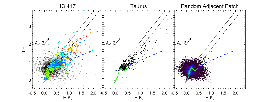
Figure 21: $JHK_{s}$ color-color diagrams. Left: the IC 417 sample, as in Figure 11 above. Small black dots are the ensemble catalog, and larger dots are the YSO candidates. Targets ranked 5 (highest) are blue, 4 are cyan, 3 are green, 2 are orange, and 1 (lowest) are red; the bluer the symbol, the more reliable a YSO candidate it is. Center: Taurus sample of confirmed YSOs. Right: randomly selected adjacent patch of sky near IC 417 – e.g., there are unlikely to be YSOs here. In this panel, colors correspond to point density with black/purple being the lowest number of points and orange/red being the highest (the highest density bins are in this case hidden under the green ZAMS line). For all three plots, reddening vectors (following the reddening law from Indebetouw et al. 2008 and Mathis 1990) are as shown. Green solid lines are the expected (empirical) ZAMS relationship. The ZAMS is taken from Pecaut & Mamajek (2013), the dashed blue line is the Meyer et al. (1997) T Tauri locus, and the dash-dot lines are reddening vectors extending roughly from the green ZAMS relation to give an indication of which of these stars could be reddened MS stars. Young stars should be clustered near the T Tauri locus and up and to the right, and the Taurus sample is found there. The IC 417 YSO candidate sample is clearly more like the Taurus sample than the targets found in the adjacent patch of sky.

$J-H$ vs. $H-K_{s}$, Fig. 21. In the $JHK_{s}$ diagram, the distribution of Taurus YSOs suggests they are nearly all low-mass (few are located in positions close to the high-mass end of the ZAMS as shown), some having large enough IR excesses so as to affect the $JHK_{s}$ colors (some near the T Tauri locus), and many subject to high $A_{V}$ (smeared up and to the right of the ZAMS and the T Tauri locus). The Taurus stars are located where YSOs are expected to be found in this diagram. The random patch of sky has a significant blob of stars clumped at the ZAMS, very few (in terms of fraction or absolute number) stars apparently reddened, and very few (in terms of fraction or absolute number) stars near the T Tauri locus. In contrast, the IC 417 sample has many high-quality YSO candidates clustered around the ZAMS, both the high- and low-mass ends, some near the T Tauri locus, and many subject to high $A_{V}$. The most outlying points in this diagram tend to be the low-ranking YSO candidates. It is not surprising that IC 417 has more high-mass stars than Taurus; Taurus is known to have few high-mass stars. The higher-quality YSO candidates bear a far stronger resemblance to the Taurus sample than the random sky sample.

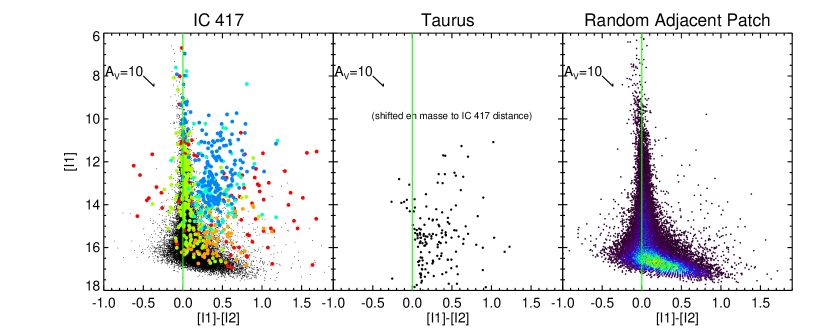
Figure 22: IRAC color-magnitude diagrams, with notation as in Figure 21. Left: the IC 417 sample. Small black dots are the ensemble catalog, and larger dots are the YSO candidates, where the bluer the symbol color, the more reliable a YSO candidate it is. Center: Taurus sample of confirmed YSOs, shifted to be at 2 kpc, the distance of IC 417. Right: randomly selected adjacent patch of sky near IC 417 – e.g., there are unlikely to be YSOs here. In this panel, colors correspond to point density with black/purple being the lowest number of points and orange/red being the highest. For all three plots, reddening vectors (following the reddening law from Indebetouw et al. 2008 and Mathis 1990) are as shown. The green solid line is the expected color for main sequence stars. Young stars should generally be found significantly to the right of the green line, and the Taurus sample is found there. The IC 417 YSO candidate sample is clearly more like the Taurus sample than the background stars found in the adjacent patch of sky.

[I1] vs. [I1]$-$[I2], Fig. 22. The IRAC color-magnitude diagram is the best here in terms of both containing most of the target stars and being least sensitive to reddening. The Taurus sample in the Figure has been shifted out to 2 kpc for more direct comparison to IC 417, where it becomes clear, again, that Taurus has few high mass stars. Many – but not all – of the Taurus stars have significant IR excesses in this diagram; that is, they are significantly to the right of the green line. Not all of the Taurus stars have excesses in this diagram because some have IR excesses that start at wavelengths longer than 4.5 $\mu$m, and some do not have IR excesses. The Taurus stars are located where YSOs are expected to be found in this diagram. Relatively few of the stars in the random patch of sky are significantly to the right of the green line. IC 417’s highest quality YSO candidates for the most part have IR excesses; that is, they are largely significantly to the right of the green line. Some of the lower quality YSO candidates have smaller excesses in this diagram. Many of the lowest quality YSO candidates are extreme outliers in this diagram, some in the unphysical location far to the left of the green line. The higher-quality YSO candidates bear a far stronger resemblance to the Taurus sample than the random sky sample.

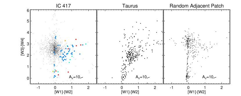
Figure 23: WISE color-color diagrams. Left: the IC 417 sample, with notation as in Figure 21. Small black dots are the ensemble catalog, and larger dots are the YSO candidates, where the bluer the symbol color, the more reliable a YSO candidate it is. Center: Taurus sample of confirmed YSOs. Right: randomly selected adjacent patch of sky near IC 417 – e.g., there are unlikely to be YSOs here. For all three plots, reddening vectors (following the reddening law from Indebetouw et al. 2008 and Mathis 1990) are as shown. Main sequence stars should have zero color in this plot. Young stars should be red, up and to the right in this plot, and the Taurus sample is found there. The IC 417 YSO candidate sample is clearly more like the Taurus sample than the background stars found in the adjacent patch of sky.

[W3]$-$[W4] vs. [W1]$-$[W2], Fig. 23. Like the IRAC color-magnitude diagram, this WISE color-color diagram is not very sensitive to the effects of reddening, but a low fraction of our stars have detections at all four WISE bands, in no small part because IC 417 is at $\sim$2 kpc. Since Taurus is only $\sim$140 pc away, most of the Taurus stars have detections at all four WISE bands. The Taurus WISE plot is well-populated. The stars without circumstellar disks have colors near zero; the stars with large IR excesses (and therefore likely circumstellar disks) are distributed up and to the right from that (0,0) locus. The Taurus stars are located where YSOs are expected to be found in this diagram. The targets in the random patch of sky include a locus of dust-free stars at (0,0), and then a clump near (0,3) that are likely background galaxies seen through the outer galaxy. The distribution of targets to the right, with both [W1]$-$[W2] and [W3]$-$[W4] greater than $\sim$0.5 or 1 mags, plausibly have colors consistent with YSOs, as can be seen in comparison to the Taurus plot. However, the overall distribution of Taurus YSOs looks far different than the overall distribution from the random patch of sky. IC 417’s highest quality YSO candidates are primarily in the right part of the diagram to be consistent with the concentration of Taurus YSOs near ($\sim$1, $\sim$2). Some have smaller excesses in [W1]$-$[W2] and/or [W3]$-$[W4] than most YSOs. The background stars in IC 417 look like the background stars in the random patch of sky, except that they are not quite as red in [W3]$-$[W4]. Several of the lowest quality YSO candidates are extreme outliers in this diagram. The higher-quality YSO candidates bear a stronger resemblance to the Taurus sample than to the background or the random sky sample.

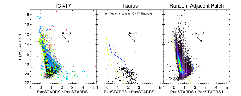
Figure 24: PanSTARRS $z$ vs. $r-i$ color-magnitude diagrams, with notation as in Figure 21. Left: the IC 417 sample. Small black dots are the ensemble catalog, and larger dots are the YSO candidates, where the bluer the symbol color, the more reliable a YSO candidate it is. Center: Taurus sample of confirmed YSOs, shifted to be at 2 kpc, the distance of IC 417. Right: randomly selected adjacent patch of sky near IC 417 – e.g., there are unlikely to be YSOs here. In this panel, colors correspond to point density with black/purple being the lowest number of points and orange/red being the highest. For all three plots, reddening vectors (following the reddening law from Indebetouw et al. 2008 and Mathis 1990) are as shown. The blue and yellow dashed lines are 6 Myr and 9 Myr isochrones from PARSEC models (Bressan et al. 2012), respectively. Young stars should be clustered around the isochrone corresponding to their age, but there is a fundamental degenerate uncertainty between age and distance, further complicated by reddening. The distance to Taurus is well known, but the distance to IC 417 is much less well known. The IC 417 YSO candidates hug the isochrones and are largely found between the two isochrones, as the Taurus stars are.

Pan-STARRS $z$ vs. $r-i$, Fig. 24. This is the first optical diagram considered here, and the reddening is now a bigger concern than in the IR diagrams above. The Taurus sample is again shifted out to 2 kpc for a fairer comparison to IC 417. Most of the Taurus stars hug the 6 Myr isochrone, which is where YSOs are expected to be in this diagram, at least for YSOs of about that age. It is apparent that there are no high-mass stars in Taurus, and that there is considerable scatter in the data, since so many Taurus YSOs appear below the 9 Myr isochrone in this plot. This is likely due not only to observational uncertainties but also reddening corrections (or lack thereof). The random patch of sky looks much different than the Taurus YSO sample. The locus where there are the most stars is closest to the 9 Myr isochrone, but is not terribly well-aligned with it. There are two ‘prongs’ near $z\sim 14$; the bluer one is from main sequence stars, and the redder one comes from reddened background giants, smeared by reddening down to their current observed location. There is a fundamental degeneracy in the uncertainties here – there is likely an age spread in the star formation regions, and probably a range of distances as well. If we don’t know the distance well to any young cluster, we can only poorly constrain the age of said young cluster, because both age and distance slide the isochrones up and down in this diagram, and reddening only worsens these uncertainties. Taurus is close, and well-studied; IC 417 is far and not well-studied. The IC 417 highest quality YSO candidates hug the 6 Myr isochrone; the lower quality YSO candidates are dispersed more broadly between the 6 and 9 Myr isochrones, as are the Taurus stars. The YSO candidates that are most likely to be giants are the ones near the reddening vector annotation, and those are most often the lowest-ranking YSO candidates. The higher-quality YSO candidates bear a stronger resemblance to the Taurus sample than to the random sky sample.

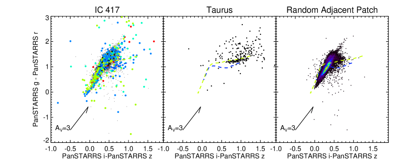
Figure 25: PanSTARRS $griz$ color-color diagrams, with notation as in Figure 21. Left: the IC 417 sample. Small black dots are the ensemble catalog, and larger dots are the YSO candidates, where the bluer the symbol color, the more reliable a YSO candidate it is. Center: Taurus sample of confirmed YSOs. Right: randomly selected adjacent patch of sky near IC 417 – e.g., there are unlikely to be YSOs here. In this panel, colors correspond to point density with black/purple being the lowest number of points and orange/red being the highest. For all three plots, reddening vectors (following the reddening law from Indebetouw et al. 2008 and Mathis 1990) are as shown. The blue and yellow dashed lines are 6 Myr and 9 Myr isochrones from PARSEC models (Bressan et al. 2012), respectively. Young stars should be near the isochrones, but the reddening complicates things here, as reddening pushes things up and to the right in this plot. Stars with large blue excesses from accretion will be found below the isochrones. Some Taurus stars are found there, as are some IC 417 stars. As noted in the text, this was not as effective a way to find YSOs as we’d hoped.

Pan-STARRS $g-r$ vs. $i-z$, Fig. 25. This optical color-color diagram incorporates the shortest wavelengths to which we have access, and as a result, it is most sensitive to reddening and has the most scatter of all the diagrams we used. Stars with a significant blue excess (like YSOs with significant blue excess due to accretion) should appear in the lower half of this diagram. What makes this hard is that reddening acts to push the stars up, out of the regime of obvious blue excess, and star forming regions have considerable, often patchy, dust creating reddening. The Taurus sample shows this clearly; there are a few stars clearly below the blue isochrone, but there are lot more scattered up and to the right as a result of reddening. The random patch of sky has stars largely around the isochrones, with some smearing up and to the right due to reddening. There are fractionally fewer stars smeared up and to the right than in the Taurus sample, because fractionally fewer stars are subject to substantial reddening in the random patch of sky. There are a few stars that appear to have a blue excess in the random patch of sky, and these plausibly could be active stars. The IC 417 YSO candidate sample in this parameter space is not as dramatically similar to Taurus and different from the random patch of sky than it was in the earlier figures, but there are still some important characteristics to note. Some YSO candidates are in the region of blue excesses, and some are in the region of highly reddened stars. Most, however, are consistent with where the ensemble of background stars are found. As noted in the main body of the paper, this color-color diagram is not as effective here as others for identifying YSO candidates.

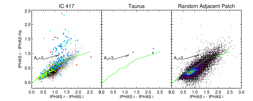
Figure 26: IPHAS $riH\alpha$ color-color diagrams, with notation as in Figure 21. Left: the IC 417 sample. Small black dots are the ensemble catalog, and larger dots are the YSO candidates, where the bluer the symbol color, the more reliable a YSO candidate it is. Center: Taurus sample of confirmed YSOs (only 4 stars were observed by IPHAS). Right: randomly selected adjacent patch of sky near IC 417 – e.g., there are unlikely to be YSOs here. In this panel, colors correspond to point density with black/purple being the lowest number of points and orange/red being the highest. For all three plots, reddening vectors (following the reddening law from Indebetouw et al. 2008 and Mathis 1990) are as shown. The IPHAS ZAMS is shown in green and is from Drew et al. (2005). The IPHAS data appear quantized due to the precision with which the magnitudes are reported in H$\alpha$. Young stars that are bright in H$\alpha$ will be above the ZAMS. Many more IC 417 stars are found there than stars from the random patch of sky.

IPHAS $r-H\alpha$ vs. $r-i$, Fig. 26. This optical diagram is the hardest to compare across samples because we do not have these data for Taurus. Stars that are bright in H$\alpha$ due to accretion, e.g., YSOs, will appear in the upper half of this diagram, above the ZAMS shown. The targets from the random patch of sky have fractionally very few stars in the top half of this diagram; the overwhelming majority of the stars are clustered near the ZAMS and smeared from there along the reddening vector. The IC 417 high-quality YSO candidate sample has many stars very bright in $r-H\alpha$ (in the top half of the diagram, e.g., where YSOs are expected to be). There are also many YSO candidates consistent with ZAMS colors. The higher-quality YSO candidates include many clearly significantly different from the random sky sample.

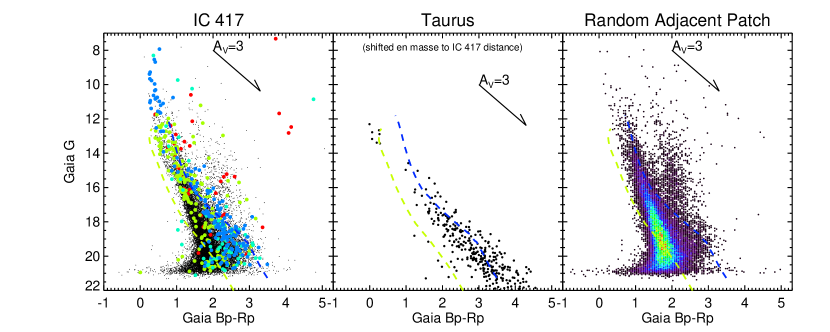
Figure 27: Gaia $G$ vs. $G_{BP}-G_{RP}$ color-magnitude diagrams, with notation as in Figure 21. Left: the IC 417 sample. Small black dots are the ensemble catalog, and larger dots are the YSO candidates, where the bluer the symbol color, the more reliable a YSO candidate it is. Center: Taurus sample of confirmed YSOs, shifted en masse to be at 2 kpc, the distance of IC 417. Right: randomly selected adjacent patch of sky near IC 417 – e.g., there are unlikely to be YSOs here. In this panel, colors correspond to point density with black/purple being the lowest number of points and orange/red being the highest. For all three plots, reddening vectors (following the reddening law from Indebetouw et al. 2008 and Mathis 1990) are as shown. The blue and yellow dashed lines are 6 Myr and 9 Myr isochrones from PARSEC models (Bressan et al. 2012), respectively. Young stars should be clustered around the isochrone corresponding to their age, but there is a fundamental degenerate uncertainty between age and distance, further complicated by reddening. The distance to Taurus is well known, but the distance to IC 417 is much less well known. The IC 417 YSO candidates hug the isochrones and are largely found between the two isochrones. The Taurus stars do a better job of clustering around the 6 Myr isochrone.

Observed Gaia DR3 $G$ vs. $G_{BP}-G_{RP}$, Fig. 27. This optical color-magnitude diagram is similar to the Pan-STARRS $z$ vs. $r-i$ diagram above, but has less scatter overall. The Taurus sample is again shifted out to 2 kpc for a fairer comparison to IC 417. Most of the Taurus stars hug the 6 Myr isochrone, which is where YSOs are expected to be in this diagram, at least for YSOs of about that age. Note that there are stars scattered down between and below the isochrones, likely due to reddening. The random patch of sky has the two ‘prongs’ (as in Fig. 24), and the highest density of points is most consistent with the oldest isochrone but is not well-matched to it. The IC 417 YSO candidate sample is clustered around the 6 Myr isochrone, including some high mass stars. The stars that are most likely giants (e.g., those appearing near the reddening vector annotation) are lowest ranking YSO candidates. The higher-quality YSO candidates bear a stronger resemblance to the Taurus sample than to the random sky sample.

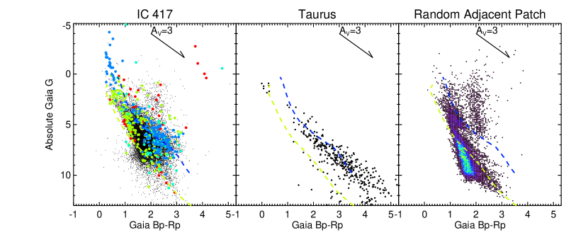
Figure 28: Gaia absolute $G$ vs. $G_{BP}-G_{RP}$ color-magnitude diagrams, with notation as in Figure 21. Left: the IC 417 sample, as in Figure 11 above. Small black dots are the ensemble catalog, and larger dots are the YSO candidates, where the bluer the symbol color, the more reliable a YSO candidate it is. Center: Taurus sample of confirmed YSOs. Right: randomly selected adjacent patch of sky near IC 417 – e.g., there are unlikely to be YSOs here. In this panel, colors correspond to point density with black/purple being the lowest number of points and orange/red being the highest. For all three plots, reddening vectors (following the reddening law from Indebetouw et al. 2008 and Mathis 1990) are as shown. The blue and yellow dashed lines are 6 Myr and 9 Myr isochrones from PARSEC models (Bressan et al. 2012), respectively. Young stars should be clustered around the isochrone corresponding to their age, but there is a fundamental degenerate uncertainty between age and distance, further complicated by reddening. The distance to Taurus is well known, but the distance to IC 417 is much less well known. The IC 417 YSO candidates hug the isochrones and are largely found between the two isochrones. The Taurus stars do a better job of clustering around the 6 Myr isochrone. The random patch of sky has no similar clustering.

Absolute Gaia DR3 $G$ vs. $G_{BP}-G_{RP}$, Fig. 28. This absolute color-magnitude diagram is another version of the prior optical color-magnitude diagram, but now with everything shifted to 10 pc. As before, the Taurus sample is well-clustered around the 6 Myr isochrone, but with some stars scattered down between and below the isochrones. The random patch of sky still has two ‘prongs’ (the one due to giants is now more distinct from that due to MS stars, making the effects of reddening far more obvious), and its densest portion is kind of close to the 9 Myr isochrone. The IC 417 YSO candidates cluster around the 6 Myr isochrone, with some scatter down between and below the isochrones. The stars that are most likely to be giants are the least confident YSO candidates. The higher-quality YSO candidates bear a stronger resemblance to the Taurus sample than to the random sky sample.

Appendix D Brief Examples of Source Ranking

Figure 10 shared twelve example SEDs; we now briefly discuss each of them in turn with an explanation of their final rank. The color-color and color-magnitude diagrams from the prior section (App C) are included here in two pairs of figures where the twelve stars are highlighted. Figs. 29 and 30 have: 1-J052807.89+341842.1; 2-J052858.77+342232.5; 3-J052718.35+344033.4; 4-J052736.37+344940.6; 5-J052705.83+343312.0; and 6-J052708.88+345031.5. Figs. 31 and 32 have: 7-J052717.77+342601.1; 8-J052743.82+344028.0; 9-J052919.14+341747.1; 10-J052825.85+342309.6; 11-J052807.15+342732.3; and 12-J052811.74+341625.0.

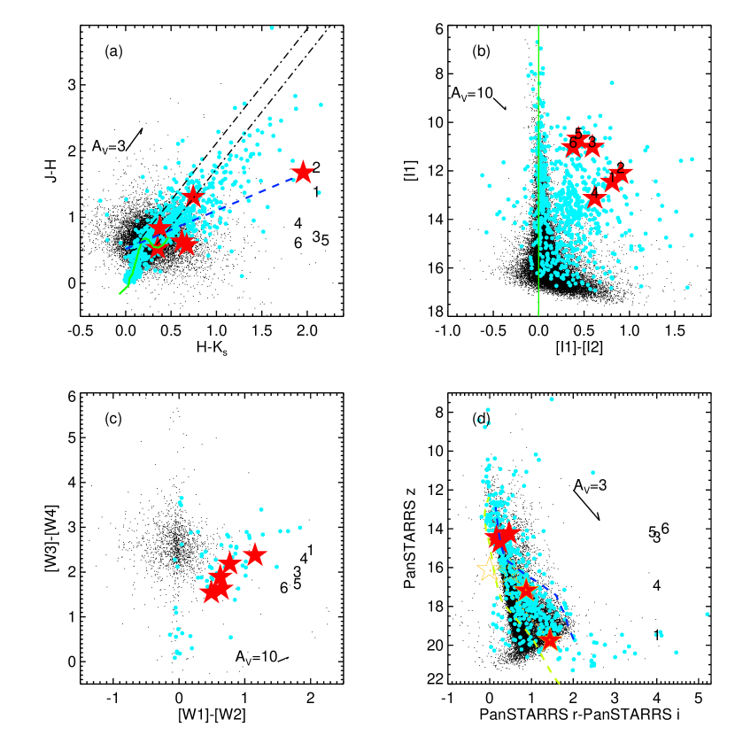
Figure 29: Color-color and color-magnitude diagrams for the first six sources in §D (red stars). Black numbers in each panel correspond to the source numbers here in the text; in panel b the numbers are on the corresponding symbols, but in panels a, c, and d, they are offset to the right hand side for clarity, but are aligned in roughly the same orientation as the symbols. Black points are the entire IC 417 catalog, cyan points are the YSO candidates. As in earlier similar plots, green lines (where they appear) are ZAMS, blue/yellow dashed lines (where they appear) are PARSEC isochrones, and reddening vectors are computed as described in the text. The individual reddening, where possible, was estimated from the star’s placement in the $JHK_{s}$ (first panel) and applied in the optical color-magnitude diagram (last panel); the offset orange hollow star is where the star would appear if dereddened according to the assumed reddening law and $JHK_{s}$-derived magnitude.

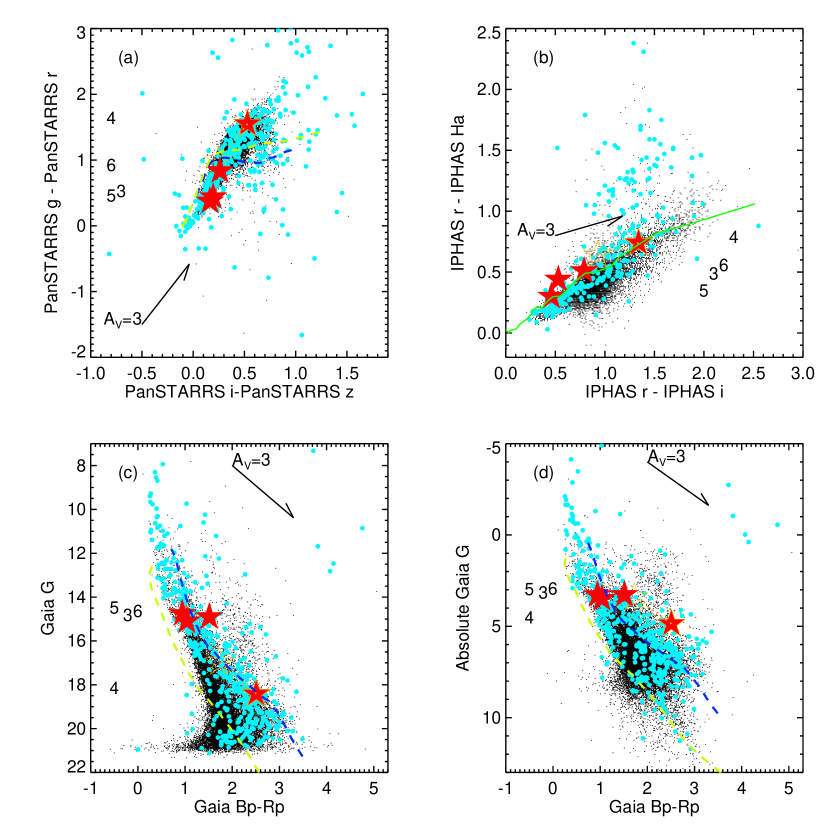
Figure 30: Color-color and color-magnitude diagrams for the first six sources in §D (red stars). Notation is as in previous figure.

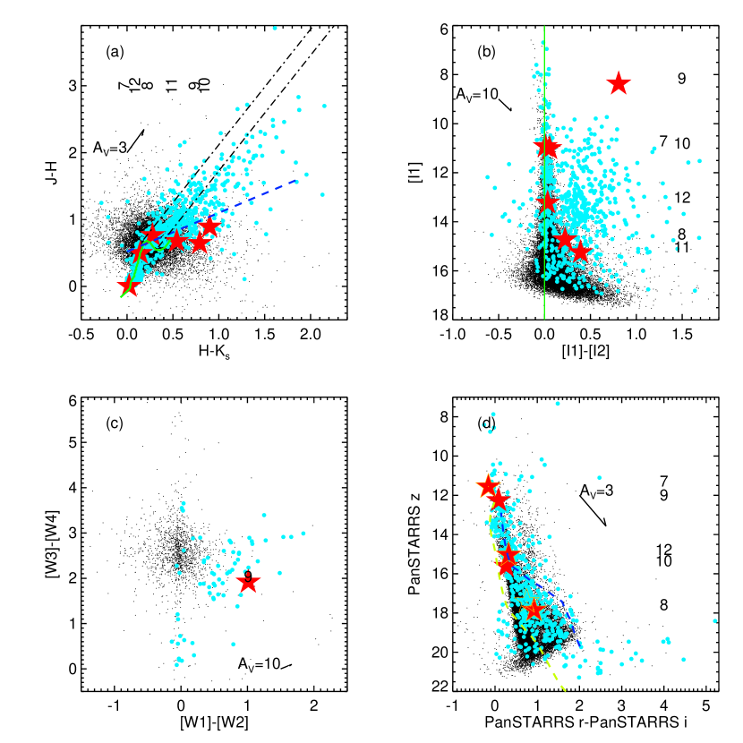
Figure 31: Color-color and color-magnitude diagrams for the second six sources in §D (red stars). Notation is as in previous figure, except the source numbers in panel a are along the top rather than along the side.

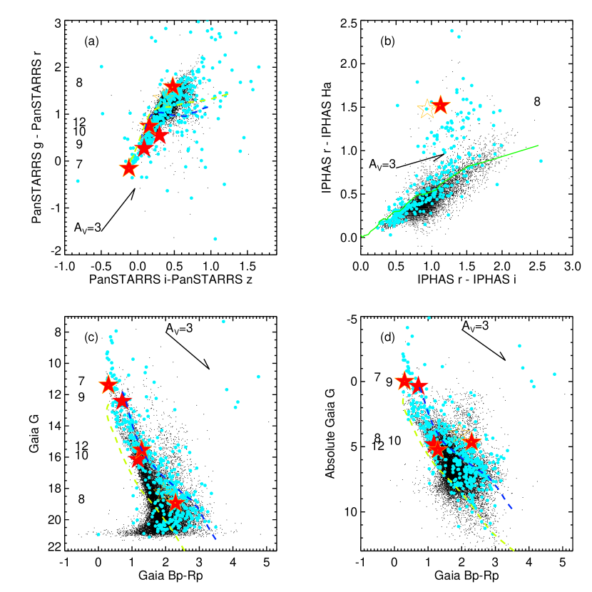
Figure 32: Color-color and color-magnitude diagrams for the second six sources in §D (red stars). Notation is as in previous figure.

Source J052807.89+341842.1 has a final rank 5 and is SED Class I. (It is star 1 in Fig. 29 and is too faint to appear in Fig. 30.) It was selected as a YSO by Pandey et al. (2020) and Winston et al. (2020), and independently by us based on WISE IR excess. Its SED shows an unambiguous, large IR excess. The reddening as calculated from $JHK_{s}$ suggests $A_{V}$ of nearly 7 magnitudes, but the $JHK_{s}$ diagram indicates that the circumstellar disk is not strongly affecting the near-IR. It appears in the right place to be a YSO (e.g., large IR excesses) in panels b and c of Fig. 29; it is very faint in panel d, consistent with $A_{V}$$\sim$7 mag. It is highly likely that this is a legitimate YSO.

Source J052858.77+342232.5 has a final rank 4 and, like the prior source, is SED Class I. (It is star 2 in Fig. 29 and, also like the prior source, is too faint to appear in Fig. 30.) It is within the NS polygon (in projection on the sky). It was selected by Winston et al. (2020) as a YSO, and independently by us based on WISE IR excess. Like the prior source, it has an unambiguous, large IR excess in the SED. However, this source has fewer points delineating its SED, which is the primary reason it has a lower final ranking, 4, than the previous source. It appears in Fig. 29, panel a, as being in the right place to have its $JHK_{s}$ affected by IR excess due to a circumstellar disk. It appears in the right place to be a YSO (e.g., large IR excesses) in panels b and c. It is too faint to appear in panel d.

Source J052718.35+344033.4 is another final rank 5, but this is an SED Class flat. (It is star 3 in Figs. 29 and  30.) It was selected by Winston et al. (2020) as a YSO, and independently by us based on WISE IR excess; it has an unambiguous IR excess. Looking at the SED, it seems like this source might have an H$\alpha$ excess, but the size of the error bars suggests that this is not a significant excess (e.g., $\chi_{\rm{IPHAS}}<3$). In Fig. 29, panel a, it appears within the ‘pack’ of stars clumped near the ZAMS. In panel b, it has an excess, but it doesn’t have enough WISE data to appear in panel c. In panel d, it is consistent with the 6 Myr isochrone. In all four of the panels in Fig. 30, it is consistent with the ‘pack’ of stars near the ZAMS. In panel b, upon close inspection, it is indeed slightly above the ZAMS, but given the errors, it’s not significantly above the ZAMS. The Gaia parallax and distance is exactly right for IC 417.

Source J052736.37+344940.6 is another SED flat Class, but this is a final rank 4. (It is star 4 in Figs. 29 and 30.) It was selected by Winston et al. (2020) as a YSO. It has a clear IR excess in the SED. In Fig. 29, panel a, it appears within the ‘pack’ of stars clumped near the ZAMS, but its position suggests some reddening ($A_{V}$$\sim$1.8 mag); panels b and c show that it is in the right place to be a YSO. Panel d also has it in the right place to be a $\sim$6 Myr old YSO; the reddening correction moves it slightly closer to the 6 Myr isochrone. It has enough PanSTARRS data to have it appear in Fig. 30, panel a, but the reddening pushes it significantly up and to the right. It is on the ZAMS in panel b, and on the 6 Myr isochrone in panel c. Panel d, however, which is the absolute Gaia CMD, has this star a little high. The Gaia data suggest it may be a little too far – Bailer-Jones et al. (2021) have a distance of 5148 pc, Gaia DR3 has 14,750 pc, but a parallax whose error bars comfortably overlap with the expected parallax range for IC 417. Based on the large IR excess, it is probably young, but based on the distance, we have placed it as a 4, not a 5.

Source J052705.83+343312.0 is final rank 5, SED Class II. (It is star 5 in Figs. 29 and 30.) It is in our list because it was selected by Winston et al. (2020) as a YSO, and independently by us based on WISE IR excess; it clearly has an IR excess in its SED. In Fig. 29, panel a, for its $J-H$, it is fairly blue in $H-K_{s}$, so as to render it impossible to estimate reddening using our approach, since no amount of reddening will move this back to the ZAMS. Fig. 29, panels b and c show that it is in the right place to be a YSO. Panel d suggests that it is on the 6 Myr isochrone, and suggests that perhaps it is a higher mass star than many of the other stars in the entire sample. Fig. 30, panels a and b also places this star in a relatively high-mass location. This is another one where the SED and even its placement in panel b seems like it may also have an H$\alpha$ excess, but the size of the error bars suggests that this is not a significant excess. Fig. 30 panels c and d are the Gaia CMDs; in both, this star is in between the two isochrones. It is at the right distance to be in IC 417. Given all of this, we ranked it as a 5. Interestingly, Gaia DR3 reports that this is an eclipsing binary, but the Zwicky Transient Facility (ZTF; Bellm et al. 2019) light curve for it reveals that it is not a binary, but rather much more likely to be a dipper (e.g., Cody et al. 2014 and references therein) – these stars have large downward excursions likely due to eclipses by dust in the inner disk. We will explore the ZTF light curves more for these target stars in a future paper.

Source J052708.88+345031.5 is another final rank 5, SED Class II. (It is star 6 in Figs. 29 and 30.) It was selected as a YSO by Pandey et al. (2020) and Winston et al. (2020), and independently by us based on WISE IR excess. It has substantial IR excess, but not significant H$\alpha$ excess. It is essentially on the ZAMS in Fig. 29, panel a, and in the regions with IR excesses in panels b and c. In panel d, it is a little above the 6 Myr isochrone. In Fig. 30, panel a, it is in the ‘pack’ of stars near the isochrones; it is marginally above the ZAMS in panel b (consistent with not being significantly above the ZAMS). In both panels c and d, it is a little above the 6 Myr isochrone, as for the prior figure. It is at the right distance to be in IC 417.

Source J052717.77+342601.1 is also known as LS V +34 13; it is a final rank 5, SED Class III. (It is star 7 in Figs. 31 and 32.) It is identified as a B2IV by MN16. Gaia DR3 says that it is a white dwarf, but the SED supports it being likely an O or B star. It is therefore likely young. There is not much reddening towards this star; Fig. 31, panel a shows it at the right place to be an unreddened early-type star. Panel b suggests that it does not have an IR excess in IRAC bands, and it doesn’t have all four WISE bands, so it cannot appear in panel c. Fig. 31 panel d and Fig. 32 panel a both again place it consistent with being a high-mass young star. It does not have enough IPHAS data to appear in panel b. Panels c and d both have it high in the diagram, beyond the end of the isochrones. It is at the right distance to be in IC 417.

Source J052743.82+344028.0 is a final rank 4, SED Class III. (It is star 8 in Figs. 31 and 32.) It was identified by Witham et al. (2008) as an H$\alpha$-bright star, and that is obvious even in the SED. It does not appear to have much of an IR excess; if it does have an IR excess, it is small, and determining the size of such an excess would require a spectral type. There is not much reddening towards this star; Fig. 31, panel a, shows it very close to the ZAMS, and the inferred reddening is $A_{V}$$\sim$0.8 mag. In panel b, this star is within the broad ‘pack’ of stars at the faint end of the distribution where the errors get larger. It doesn’t appear in panel c. It is faint in panel d, and appears between the isochrones. In Fig. 32, panel a, it is clearly reddened to be above the isochrones. In panel b, it is obviously and unambiguously bright in H$\alpha$. In panels c and d, it is faint and between the isochrones. The Gaia DR2 Bailer-Jones distance is ok (2192 pc), the DR3 Bailer Jones distance is slightly too far (7249 pc), and the Gaia DR3 distance is ok (3085 pc). Because of this ambiguity, and since the sole indicator of youth, per se, is the H$\alpha$ excess, which could also just be an indicator of elevated stellar activity, we have ranked this star a 4 rather than a 5.

Source J052919.14+341747.1 is one of the most peculiar oddballs with final rank 4*. It is SED Class flat, and star 9 in Figs. 31 and 32.) It was identified in J08 as having H$\alpha$ excess and was flagged in Winston et al. (2020) and Pandey et al. (2020) as a YSO, as did we in our initial WISE IR excess search. Its SED is unlike most YSO SEDs; it has MSX, AKARI, and PACS counterparts that all appear to be consistent. In Fig. 31, panel a it seems to be so blue in $H-K_{s}$ given its $J-H$ that guessing a reddening value is not easy. It is very bright in panel b, with a large IR excess; it also is the only one of this set to appear in panel c. It is on the isochrone and consistent with a high-mass star in Fig. 31, panel d as well as Fig. 32, panel a. It does not have IPHAS data so it does not appear in panel b. In panels c and d, it is on the isochrone consistent with a 6 Myr star. It has a Gaia DR3 distance completely consistent with IC 417. A spectrum is needed to understand this object.

Source J052825.85+342309.6 is another oddball with final rank 4*; it is SED Class II (and star 10 in Figs. 31 and 32). It was identified in J08 as having H$\alpha$ excess and in Winston et al. (2020) as a YSO. Its SED is unlike most YSO SEDs; it is too broad. In Fig. 31, panel a, it appears to be in the T Tauri locus. In panel b, it appears to not have much of an IR excess at IRAC bands, and does not have enough data to appear in panel c. It is between the isochrones in panel d. In Fig. 32 it is consistent with possibly having a small blue excess. It does not have enough data to appear in panel b. In panel c, it is between the isochrones, but in panel d, it is a little above the 6 yr isochrone. Nonetheless, it has a Gaia DR3 distance completely consistent with IC 417. A spectrum is needed to understand this object.

Source J052807.15+342732.3 is final rank 2, SED Class II. (It is star 11 in Fig. 31 and does not have enough data for Fig. 32.) It is on our list of candidate YSOs because it was identified as such in J17. In Fig. 31, panel a, it is either on the reddest portion of the ZAMS or the bluest portion of the T Tauri locus. It is faint, but has an IR excess in panel b; it does not appear in panel c or d. It is low-ranked primarily because it has so few points in its SED compared to others on our list, though it does seem to have an IR excess.

Finally, J052811.74+341625.0 is final rank 3, SED Class III. (It is star 12 in Figs. 31 and 32.) It is identified as a variable in Lata et al. (2019), but that variability is the only indication of youth. Fig. 31, panel a has it on the ZAMS with very little reddening. Panel b shows no IR excess; it does not appear in panel c. It is on the 6 Myr isochrone in panel d. In Fig. 32, it is on the isochrones in panel a. It does not appear in panel b. In panel c, it is on the 6 Myr isochrone; in panel d, it is between the isochrones. Gaia DR3 says that it is at the right distance to be in IC 417, so it is a rank 3.

A complete set of SEDs has been delivered to IRSA, along with the complete data table (Table 4), which includes ranks, flags, and photometry.

References

- AKARI team (2010a) AKARI team, 2010a, AKARI/FIS All-Sky Survey Bright Source Catalogue, IRSA, doi:10.26131/IRSA180
- AKARI team (2010b) AKARI team, 2010b, AKARI/IRC Point Source Catalogue, IRSA, doi:10.26131/IRSA181
- Alcala et al. (1996) Alcala, J. M., Terranegra, L., Wichmann, R., et al. 1996, A&AS, 119, 7
- Andrae et al. (2022) Andrae, R., Fouesneau, M., Sordo, R., et al. 2022, arXiv:2206.06138
- Bailer-Jones et al. (2018) Bailer-Jones, C. A. L., Rybizki, J., Fouesneau, M., et al. 2018, AJ, 156, 58. doi:10.3847/1538-3881/aacb21
- Bailer-Jones et al. (2021) Bailer-Jones, C. A. L., Rybizki, J., Fouesneau, M., et al. 2021, AJ, 161, 147. doi:10.3847/1538-3881/abd806
- Barentsen et al. (2014) Barentsen, G., Farnhill, H. J., Drew, J. E., et al. 2014, MNRAS, 444, 3230. doi:10.1093/mnras/stu1651
- Barnbaum et al. (1996) Barnbaum, C., Stone, R. P. S., & Keenan, P. C. 1996, ApJS, 105, 419. doi:10.1086/192323
- Bellm et al. (2019) Bellm, E. C., Kulkarni, S. R., Graham, M. J., et al. 2019, PASP, 131, 018002. doi:10.1088/1538-3873/aaecbe
- Bica et al. (2003) Bica, E., Dutra, C. M., Soares, J., et al. 2003, A&A, 404, 223. doi:10.1051/0004-6361:20030486
- Borissova et al. (2003) Borissova, J., Pessev, P., Ivanov, V. D., et al. 2003, A&A, 411, 83. doi:10.1051/0004-6361:20034009
- Bressan et al. (2012) Bressan, A., Marigo, P., Girardi, L., et al. 2012, MNRAS, 427, 127. doi:10.1111/j.1365-2966.2012.21948.x
- Camargo et al. (2012) Camargo, D., Bonatto, C., & Bica, E. 2012, MNRAS, 423, 1940. doi:10.1111/j.1365-2966.2012.21018.x
- Capak et al. (2013) Capak, P., 2013, Spitzer Enhanced Imaging Products (SEIP) Source List, IRSA, doi:10.26131/IRSA3
- Carpenter et al. (2001) Carpenter, J. M., Hillenbrand, L. A., & Skrutskie, M. F. 2001, AJ, 121, 3160. doi:10.1086/321086
- CatWISE team (2020) CatWISE team, 2020, CatWISE Preliminary Catalog, IPAC, doi: 10.26131/IRSA126
- Cohen et al. (2003) Cohen, M., Megeath, S. T., Hammersley, P. L., et al. 2003, AJ, 125, 2645. doi:10.1086/374362
- Chambers et al. (2016) Chambers, K., Magnier, E., Metcalf, N., et al., 2016, arXiv:1612.05560
- Chargeishvili (1988) Chargeishvili, K. B. 1988, Abastumanskaia Astrofizicheskaia Observatoriia Byulleten, 65, 18
- Chen et al. (2022) Chen, T. X., Schmitz, M., Mazzarella, J. M., et al. 2022, ApJS, 260, 5. doi:10.3847/1538-4365/ac6268
- Churchwell et al. (2009) Churchwell, E., Babler, B. L., Meade, M. R., et al. 2009, PASP, 121, 213. doi:10.1086/597811
- Cody et al. (2014) Cody, A. M., Stauffer, J., Baglin, A., et al. 2014, AJ, 147, 82. doi:10.1088/0004-6256/147/4/82
- Cody et al. (2022) Cody, A. M., Hillenbrand, L. A., & Rebull, L. M. 2022, AJ, 163, 212. doi:10.3847/1538-3881/ac5b73
- Dewangan et al. (2018) Dewangan, L. K., Baug, T., Ojha, D. K., et al. 2018, ApJ, 864, 54. doi:10.3847/1538-4357/aad4b1
- Drew et al. (2005) Drew, J. E., Greimel, R., Irwin, M. J., et al. 2005, MNRAS, 362, 753. doi:10.1111/j.1365-2966.2005.09330.x
- Efremov & Sitnik (1988) Efremov, Y., & Sitnik, T., 1988, SvAL, 14, 347
- Egan et al. (2003) Egan, T., et al., 2003, Air Force Research Laboratory Technical Report AFRL-VS-TR-2003-1589
- Eisenhardt et al. (2020) Eisenhardt, P. R. M., Marocco, F., Fowler, J. W., et al. 2020, ApJS, 247, 69. doi:10.3847/1538-4365/ab7f2a
- Evans et al. (2009) Evans, N., Calvet, N., Cieza, L., et al. 2009, arXiv:0901.1691. doi:10.48550/arXiv.0901.1691
- Fich & Blitz (1984) Fich, M. & Blitz, L. 1984, ApJ, 279, 125. doi:10.1086/161872
- Fischer et al. (2022) Fischer, W. J., Hillenbrand, L. A., Herczeg, G. J., et al. 2022, arXiv:2203.11257. doi:10.48550/arXiv.2203.11257
- Fuenmayor (1981) Fuenmayor, F. J. 1981, Rev. Mexicana Astron. Astrofis., 6, 83
- Froebrich et al. (2007) Froebrich, D., Scholz, A., & Raftery, C. L. 2007, MNRAS, 374, 399. doi:10.1111/j.1365-2966.2006.11148.x
- Gaia Collaboration et al. (2018a) Gaia Collaboration, Brown, A. G. A., Vallenari, A., et al. 2018a, A&A, 616, A1. doi:10.1051/0004-6361/201833051
- Gaia Collaboration et al. (2018b) Gaia Collaboration, Brown, A. G. A., Vallenari, A., et al. 2018b, Gaia Source Catalog DR2. doi:10.26131/IRSA12
- Gaia Collaboration et al. (2021a) Gaia Collaboration, Brown, A. G. A., Vallenari, A., et al. 2021, A&A, 649, A1. doi:10.1051/0004-6361/202039657
- Gaia Collaboration et al. (2021b) Gaia Collaboration, Brown, A. G. A., Vallenari, A., et al. 2021b, Gaia Source Catalog EDR3. doi:10.26131/IRSA541
- Gaia Collaboration et al. (2022a) Gaia Collaboration, Vallenari, A., Brown, A. G. A., et al. 2022, arXiv:2208.00211
- Georgelin et al. (1973) Georgelin, Y. M., Georgelin, Y. P., & Roux, S. 1973, A&A, 25, 337
- Getman et al. (2017) Getman, K. V., Broos, P. S., Kuhn, M. A., et al. 2017, ApJS, 229, 28. doi:10.3847/1538-4365/229/2/28
- Glimpse Team (2014) GLIMPSE Team, 2014, GLIMPSE 360 Catalog, IPAC, doi:10.26131/IRSA205
- Griffin et al. (2010) Griffin, M. J., Abergel, A., Abreu, A., et al. 2010, A&A, 518, L3. doi:10.1051/0004-6361/201014519
- Guieu et al. (2010) Guieu, S., Rebull, L. M., Stauffer, J. R., et al. 2010, ApJ, 720, 46. doi:10.1088/0004-637X/720/1/46
- Gutermuth et al. (2008) Gutermuth, R. A., Bourke, T. L., Allen, L. E., et al. 2008, ApJ, 673, L151. doi:10.1086/528710
- Gutermuth et al. (2009) Gutermuth, R. A., Megeath, S. T., Myers, P. C., et al. 2009, ApJS, 184, 18. doi:10.1088/0067-0049/184/1/18
- Herbig (1952) Herbig, G. H. 1952, JRASC, 46, 222
- Indebetouw et al. (2008) Indebetouw, R., Whitney, B. A., Kawamura, A., et al. 2008, AJ, 136, 1442. doi:10.1088/0004-6256/136/4/1442
- IRAC Instrument (2018) IRAC Instrument and Instrument Support Teams, 2021, IRAC Instrument Handbook (Pasadena, CA: Caltech/IPAC), doi:10.26131/IRSA486
- Ivanov et al. (2005) Ivanov, V. D., Borissova, J., Bresolin, F., et al. 2005, A&A, 435, 107. doi:10.1051/0004-6361:20042337
- Jayasinghe et al. (2018) Jayasinghe, T., Kochanek, C. S., Stanek, K. Z., et al. 2018, MNRAS, 477, 3145. doi:10.1093/mnras/sty838
- Joy (1945) Joy, A. H. 1945, ApJ, 102, 168. doi:10.1086/144749
- Jose et al. (2008) Jose, J., Pandey, A. K., Ojha, D. K., et al. 2008, MNRAS, 384, 1675. doi:10.1111/j.1365-2966.2007.12825.x (J08)
- Jose et al. (2017) Jose, J., Herczeg, G. J., Samal, M. R., et al. 2017, ApJ, 836, 98. doi:10.3847/1538-4357/836/1/98 (J17)
- Kiss et al. (2006) Kiss, Z. T., Tóth, L. V., Krause, O., et al. 2006, A&A, 453, 923. doi:10.1051/0004-6361:20053235
- Koenig & Leisawitz (2014) Koenig, X. P. & Leisawitz, D. T. 2014, ApJ, 791, 131. doi:10.1088/0004-637X/791/2/131
- Koenig et al. (2012) Koenig, X. P., Leisawitz, D. T., Benford, D. J., et al. 2012, ApJ, 744, 130. doi:10.1088/0004-637X/744/2/130
- Koenig et al. (2015) Koenig, X., Hillenbrand, L. A., Padgett, D. L., et al. 2015, AJ, 150, 100. doi:10.1088/0004-6256/150/4/100
- Kohoutek & Wehmeyer (1999) Kohoutek, L. & Wehmeyer, R. 1999, A&AS, 134, 255. doi:10.1051/aas:1999101
- Kronberger et al. (2006) Kronberger, M., Teutsch, P., Alessi, B., et al. 2006, A&A, 447, 921. doi:10.1051/0004-6361:20054057
- Kuhn et al. (2021) Kuhn, M. A., de Souza, R. S., Krone-Martins, A., et al. 2021, ApJS, 254, 33. doi:10.3847/1538-4365/abe465
- Lang (2014) Lang, D. 2014, AJ, 147, 108. doi:10.1088/0004-6256/147/5/108
- Lata et al. (2019) Lata, S., Pandey, A. K., Kesh Yadav, R., et al. 2019, AJ, 158, 68. doi:10.3847/1538-3881/ab298c
- Lucas et al. (2008) Lucas, P. W., Hoare, M. G., Longmore, A., et al. 2008, MNRAS, 391, 136. doi:10.1111/j.1365-2966.2008.13924.x
- Luhman (2023) Luhman, K. L. 2023, AJ, 165, 37. doi:10.3847/1538-3881/ac9da3
- Malysheva (1990) Malysheva, L. K. 1990, Soviet Ast., 34, 122
- Mamajek (2009) Mamajek, E. E. 2009, Exoplanets and Disks: Their Formation and Diversity, 1158, 3. doi:10.1063/1.3215910
- Marco & Negueruela (2016) Marco, A. & Negueruela, I. 2016, MNRAS, 459, 880. doi:10.1093/mnras/stw640
- Marocco et al. (2021) Marocco, F., Eisenhardt, P. R. M., Fowler, J. W., et al. 2021, ApJS, 253, 8. doi:10.3847/1538-4365/abd805
-
Marton et al. (2017)
Marton, G., Calzoletti L., Perez Garcia, A., Kiss, C., Paladini, R., et al., 2017, Explanatory Supplement,
http://irsa.ipac.caltech.edu/data/Herschel/PPSC/docs/HPPSC_Explanatory_Supplement.pdf - Mathis (1990) Mathis, J. S. 1990, ARA&A, 28, 37. doi:10.1146/annurev.aa.28.090190.000345
- Mayer & Macák (1971) Mayer, P. & Macák, P. 1971, Bulletin of the Astronomical Institutes of Czechoslovakia, 22, 46
-
Meade et al. (2014)
Meade, M., Whitney, B., Babler, B., Benjamin, R., Churchwell, E., Indebetouw, R., Robitaille, T., Cohen, M., 2014, GLIMPSE360 Data Description,
https://irsa.ipac.caltech.edu/data/SPITZER/GLIMPSE/doc/glimpse360_dataprod_v1.5.pdf - Meyer et al. (1997) Meyer, M. R., Calvet, N., & Hillenbrand, L. A. 1997, AJ, 114, 288. doi:10.1086/118474
- Meisner et al. (2017a) Meisner, A. M., Lang, D., & Schlegel, D. J. 2017a, AJ, 153, 38. doi:10.3847/1538-3881/153/1/38
- Meisner et al. (2017b) Meisner, A. M., Lang, D., & Schlegel, D. J. 2017b, AJ, 154, 161. doi:10.3847/1538-3881/aa894e
- Mel’Nik & Efremov (1995) Mel’Nik, A. M. & Efremov, Y. N. 1995, Astronomy Letters, 21, 10
- Mizusawa et al. (2012) Mizusawa, T. F., Rebull, L. M., Stauffer, J. R., et al. 2012, AJ, 144, 135. doi:10.1088/0004-6256/144/5/135
- Molinari et al. (2010) Molinari, S., Swinyard, B., Bally, J., et al. 2010, PASP, 122, 314. doi:10.1086/651314
- Murakami et al. (2007) Murakami, H., Baba, H., Barthel, P., et al. 2007, PASJ, 59, S369. doi:10.1093/pasj/59.sp2.S369,
- Nassau & Blanco (1954) Nassau, J. J. & Blanco, V. M. 1954, ApJ, 120, 129. doi:10.1086/145888
- Ness et al. (2016) Ness, M., Hogg, D. W., Rix, H.-W., et al. 2016, ApJ, 823, 114. doi:10.3847/0004-637X/823/2/114
- Ogura et al. (2002) Ogura, K., Sugitani, K., & Pickles, A. 2002, AJ, 123, 2597. doi:10.1086/339976
- Padgett et al. (2004) Padgett, D. L., Rebull, L. M., Noriega-Crespo, A., et al. 2004, ApJS, 154, 433. doi:10.1086/423132
- Pandey et al. (2020) Pandey, A. K., Sharma, S., Kobayashi, N., et al. 2020, MNRAS, 492, 2446. doi:10.1093/mnras/stz3596
- Pecaut & Mamajek (2013) Pecaut, M. J. & Mamajek, E. E. 2013, ApJS, 208, 9. doi:10.1088/0067-0049/208/1/9
- Pilbratt et al. (2010) Pilbratt, G. L., Riedinger, J. R., Passvogel, T., et al. 2010, A&A, 518, L1. doi:10.1051/0004-6361/201014759
- Poglitsch et al. (2010) Poglitsch, A., Waelkens, C., Geis, N., et al. 2010, A&A, 518, L2. doi:10.1051/0004-6361/201014535
- Rebull et al. (2000) Rebull, L. M., Hillenbrand, L. A., Strom, S. E., et al. 2000, AJ, 119, 3026. doi:10.1086/301393
- Rebull et al. (2007) Rebull, L. M., Stapelfeldt, K. R., Evans, N. J., et al. 2007, ApJS, 171, 447. doi:10.1086/517607
- Rebull et al. (2010) Rebull, L. M., Padgett, D. L., McCabe, C.-E., et al. 2010, ApJS, 186, 259. doi:10.1088/0067-0049/186/2/259
- Rebull et al. (2011) Rebull, L. M., Johnson, C. H., Hoette, V., et al. 2011, AJ, 142, 25. doi:10.1088/0004-6256/142/1/25
- Rebull et al. (2014) Rebull, L. M., Cody, A. M., Covey, K. R., et al. 2014, AJ, 148, 92. doi:10.1088/0004-6256/148/5/92
- Rebull et al. (2018) Rebull, L. M., Stauffer, J. R., Cody, A. M., et al. 2018, AJ, 155, 196. doi:10.3847/1538-3881/aab605
- Rebull et al. (2020) Rebull, L. M., Stauffer, J. R., Cody, A. M., et al. 2020, AJ, 159, 273. doi:10.3847/1538-3881/ab893c
- Rebull et al. (2022) Rebull, L. M., Stauffer, J. R., Hillenbrand, L. A., et al. 2022, AJ, 164, 80. doi:10.3847/1538-3881/ac75f1
- Rebull (2015) Rebull, L. M. 2015, AJ, 150, 17. doi:10.1088/0004-6256/150/1/17
- Savage et al. (1985) Savage, B. D., Massa, D., Meade, M., et al. 1985, ApJS, 59, 397. doi:10.1086/191078
- Schlafly et al. (2019) Schlafly, E. F., Meisner, A. M., & Green, G. M. 2019, ApJS, 240, 30. doi:10.3847/1538-4365/aafbea
- Skrutskie et al. (2006) Skrutskie, M. F., Cutri, R. M., Stiening, R., et al. 2006, AJ, 131, 1163. doi:10.1086/498708
- Skrutskie et al. (2003) Skrutskie, M. F., Cutri, R. M., Stiening, R., et al. 2003, 2MASS All-Sky Point Source Catalog, IPAC, doi:10.26131/IRSA2
- Slesnick et al. (2008) Slesnick, C. L., Hillenbrand, L. A., & Carpenter, J. M. 2008, ApJ, 688, 377. doi:10.1086/592265
- Stock (1956) Stock, J. 1956, ApJ, 123, 258. doi:10.1086/146158
- Vetesnik (1979) Vetesnik, M. 1979, Bulletin of the Astronomical Institutes of Czechoslovakia, 30, 1
- Walawender et al. (2006) Walawender, J., Bally, J., Kirk, H., et al. 2006, AJ, 132, 467. doi:10.1086/504638
- Werner et al. (2004) Werner, M. W., Roellig, T. L., Low, F. J., et al. 2004, ApJS, 154, 1. doi:10.1086/422992
- Wilking et al. (2001) Wilking, B. A., Bontemps, S., Schuler, R. E., et al. 2001, ApJ, 551, 357. doi:10.1086/320067
- Winston et al. (2020) Winston, E., Hora, J. L., & Tolls, V. 2020, AJ, 160, 68. doi:10.3847/1538-3881/ab99c8
- Witham et al. (2008) Witham, A. R., Knigge, C., Drew, J. E., et al. 2008, MNRAS, 384, 1277. doi:10.1111/j.1365-2966.2007.12774.x
- Wright et al. (2010) Wright, E. L., Eisenhardt, P. R. M., Mainzer, A. K., et al. 2010, AJ, 140, 1868. doi:10.1088/0004-6256/140/6/1868
- Wright et al. (2010) Wright, E. L., Eisenhardt, P. R. M., Mainzer, A. K., et al. 2010, AllWISE Source Catalog, doi:10.26131/IRSA1