Experimental Performance of Blind Position Estimation Using Deep Learning

Abstract

Accurate indoor positioning for wireless communication systems represents an important step towards enhanced reliability and security, which are crucial aspects for realizing Industry 4.0. In this context, this paper presents an investigation on the real-world indoor positioning performance that can be obtained using a deep learning (DL)-based technique. For obtaining experimental data, we collect power measurements associated with reference positions using a wireless sensor network in an indoor scenario. The DL-based positioning scheme is modeled as a supervised learning problem, where the function that describes the relation between measured signal power values and their corresponding transmitter coordinates is approximated. We compare the DL approach to two different schemes with varying degrees of online computational complexity. Namely, maximum likelihood estimation and proximity. Furthermore, we provide a performance comparison of DL positioning trained with data generated exclusively based on a statistical path loss model and tested with experimental data.

I Introduction

The growing interest for accurate indoor positioning techniques can be attributed to the increasing number of envisioned use cases for future wireless networks. As an example, enhanced emergency calls will have to provide accurate positioning services indoors for aiding rescue teams [1]. Similarly, proactive and privacy preserving localization of intentional or accidental interfering transmitters is a requirement for guaranteeing reliability and security in private wireless networks [2]. Both scenarios will benefit from positioning schemes that are able to operate with accuracy in the order of 1-5 meters in harsh propagation conditions, and with minimal prior knowledge of the transmission protocol and propagation characteristics. Therefore, indoor positioning/localization enabled by DL is expected to play a key role in future wireless networks [3, 4]. However, DL requires access to large amounts of labeled data to achieve the required performance, and this can hinder its widespread adoption.

Among the possible location-dependent signal parameters, received signal strength (RSS) and angle of arrival (AoA) allow blind localization, i.e., without previous knowledge of the transmitting protocol. For the latter case, an antenna array is required for measuring the AoA at each sensing unit (SU). However, this translates to higher implementation costs when compared to the hardware needed for RSS measurement. Moreover, the algorithms that offer high precision AoA estimation often present complexity levels that hinder real-time implementation [5]. Thus, it can be argued that RSS is the most convenient source of information for blind positioning.

In [6] we propose a blind transmitter localization framework using a deep neural network (DNN), and investigate its performance when compared to classical and state-of-the-art approaches. In this paper, we apply the approach presented in [6] to analyze the performance of DL-based positioning when real-world RSS measurements [7] are available, and to understand the achievable real-time performance by employing such technique. Furthermore, due to the significant cost associated with measurement campaigns, the localization performance is also investigated assuming synthetic data generation. The data are obtained through well accepted mathematical models that describe the relationship between the transmitters’ physical location and the corresponding RSS, i.e., statistical path loss models. This approach leverages theoretical knowledge to reduce, or completely eliminate, the need for real-world measurements.

Our contributions can be summarized as follows:

1. We validate by means of real-world measurements the DL localization approach presented in [6].

2. We analyze the performance of our DL localization scheme when the training data are synthetically generated with a PLM. This provides insights into the localization performance that can be achieved when no measured data are available, and only theoretical knowledge on propagation is used.

3. Our DL scheme is compared with other solutions of different computational complexity, namely, maximum likelihood estimator (MLE) and Proximity. The observed performance suggests that DL can provide accurate positioning using RSS as a source of position information in indoor scenarios.

The remainder of the paper is organized as follows: Section II presents the measurement setup used for data collection. Section III presents the log-normal PLM used for fitting the measured data and generating synthetic training data. Section IV describes the localization algorithms. Section V analyses the performance of the localization schemes. Finally, the paper is concluded in Section VI.

II Measurement Setup and RSS Calculation

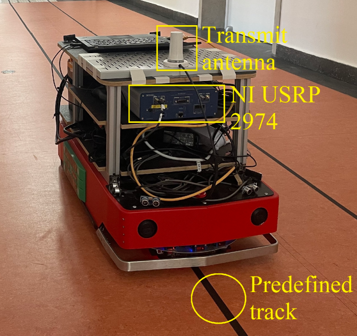
(a) Probing transmitter on the AGV.

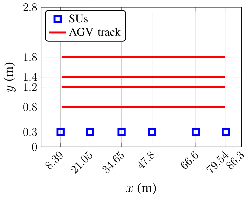
(b) Illustration of the measurement area.

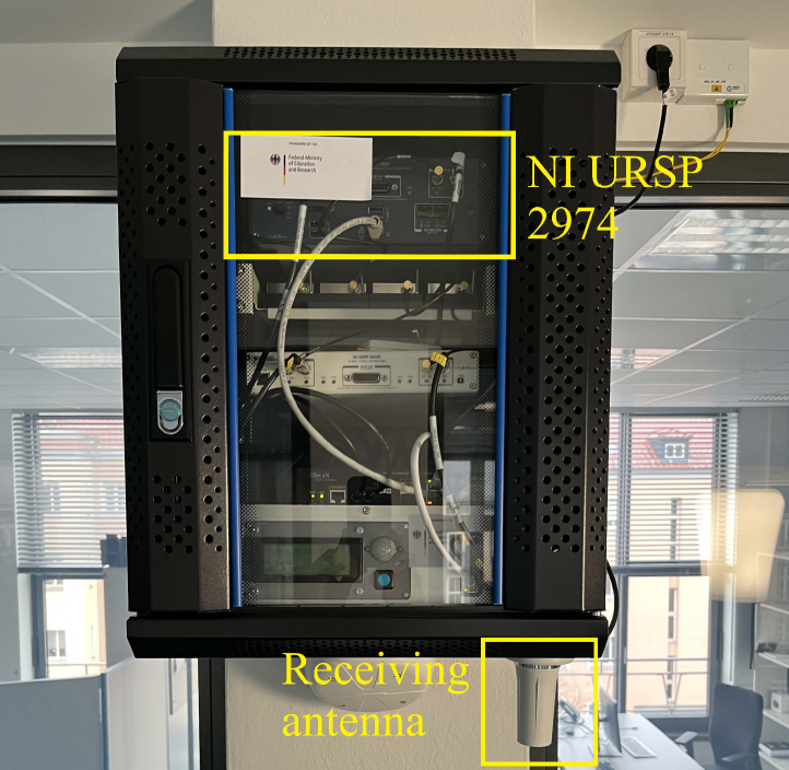
(c) One of the 6 sensing units.

Figure 1: Components employed in the measurement campaign.

The measurements are conducted using the hardware resources from the indoor Online Wireless Lab (OWL) testbed located at the Technische Universität Dresden (TUD), Dresden, Germany [8]. The indoor OWL has 6 access points mounted on the walls of an office corridor with antennas at a height of 2.5 m. These access points are configured as the SUs. A probing transmitter is carried by an automated guided vehicle (AGV) that follows a predefined track with the constant speed of 0.6 m/s. The transmit antenna is 0.5 m above the ground. Fig. 1 shows the components used in the measurement campaign with an illustration of the area where the measurements are conducted along the predefined track followed by the AGV, and the coordinates of the SUs are also shown. Both probing transmitter and SUs are implemented using the Universal Software Radio Peripheral (USRP), which is a software-defined radio (SDR) platform by National Instruments. The center frequency of operation of the radios is 3.75 GHz. The measurement environment is an indoor office hallway of size 86.3 m $\times$ 2.8 m. We define one measurement round as the AGV moves from the initial measurement point with $x_{\mathrm{init}}=9$ m until $x_{\mathrm{end}}=79.32$ m and back. The $y$ coordinates of the transmit antenna vary from 0.8, 1.2, 1.4 and 1.8 m as we place it on the right or left edges of the carrying platform on the AGV for different rounds. This is illustrated in Fig. 1(b).

The probing transmitter continuously sends a constant envelop chirp signal with 512 samples occupying a bandwidth of 100 MHz. The transmit power is set to 13 dBm. All SUs collect 5000 IQ samples at the rate of 100 Msample/s, such that one measurement period lasts 50 $\mu$s, and it is repeated every 200 ms. Consequently, the measurements are spaced apart by 12 cm. Since the AGV runs with a constant speed of 0.6 m/s, during one measurement period it moves 30 $\mu$m. Therefore, we can treat it as static within one measurement period.

In total, 4 measurement rounds have been performed during different times of the day, resulting in 4696 pairs of reference positions and the corresponding received IQ-samples. From the total pairs, 75% (3522 pairs) are reserved for training the DL model, and the remaining 25% (1174 pairs) are used as testing data. Before the split, the data are shuffled to ensure statistical reliability.

At each SU, the received IQ samples are used for calculating the RSS as follows,

$$P_{j}=10\log_{10}\left(\frac{1}{N_{y}}\sum_{n=0}^{N_{y}-1}|y[n]|^{2}\right)+30,$$ (1)

where $P_{j}$ (dBm) is the measured RSS at the $j$-th SU, and $y[n]$ represents the received signal with $N_{y}=5000$ samples.

III Path Loss and Shadowing Modeling

To generate the synthetic training data, the single slope log-normal PLM [9] has been employed. Under this model, the RSS measurement obtained at the $j$-th SU is given by

$$P_{j}=P_{0}-10\beta\log_{10}\left(\frac{d\left(\mathbf{u},\mathbf{v}_{j}\right)}{d_{0}}\right)+n_{j},$$ (2)

where $P_{0}$ (dBm) is the received power at a reference distance $d_{0}$, which includes the transmit power, and the transmit and receive antenna gains, $\beta$ is the environment dependent path loss exponent, $n_{j}$ represents the shadowing noise, $\mathbf{u}\triangleq\left[u_{x},u_{y},u_{z}\right]^{\mathrm{T}}$ and $\mathbf{v}_{j}\triangleq\left[v_{j_{x}},v_{j_{y}},v_{j_{z}}\right]^{\mathrm{T}}$ contain the transmitter and $j$-th SU coordinates in three dimensional space, respectively, and $d\left(\mathbf{u},\mathbf{v}_{j}\right)$ represents the Euclidean distance, defined as

$$\small{d\left(\mathbf{u},\mathbf{v}_{j}\right)=\sqrt{(u_{x}-v_{x_{j}})^{2}+(u_{y}-v_{y_{j}})^{2}+(u_{z}-v_{z_{j}})^{2}}.}$$ (3)

The shadowing noise experienced at the SUs is modeled by a zero-mean Gaussian random vector $\mathbf{n}$ with spatially dependent covariance matrix $\mathbf{C}\in\mathbb{R}^{N_{s}\times N_{s}}$. This accounts for the effects of signal blockage by objects in the environment and multi-path propagation. Therefore, the correlation between shadowing noise depends on the distance between SUs. Assuming an exponential correlation model [10], the covariance matrix of $\mathbf{n}$ is described as

$$\left[\mathbf{C}\right]_{a,b}=\sigma_{\mathrm{dB}}^{2}\exp\left(-\frac{d\left(\mathbf{v}_{a},\mathbf{v}_{b}\right)}{d_{\mathrm{cor}}}\right),$$ (4)

where $d_{\mathrm{cor}}$ represents the decorrelation distance, which is assumed to be 1 meter [11], and $\sigma_{\mathrm{dB}}^{2}$ the shadowing noise variance in dB.

The model described by (2) can be modified to include an extra attenuation term dependent on the number of walls or floors between transmitter and receiver. We opt to not include this term, since our experiments were carried out in a corridor without hard partitions.

IV RSS based localization techniques

Let us consider that within the area of interest, $N_{s}$ SUs are placed in fixed locations. The SUs measure RSS values and send them to a central unit (CU), where the transmitter coordinates are estimated.

IV-A Deep learning framework for blind localization

Given the data set with known transmitter positions and associated RSS measurements at fixed SUs obtained from our measurement campaign, the localization problem is modeled as a supervised learning problem. The architecture of the DNN-based transmitter localization scheme employed in this paper has been proposed in our previous work [6]. This model uses the RSS measurement vector in dB scale for numerical stability. The training process consists of an iterative minimization of a predefined loss function between the estimated and known training examples. The mean squared error (MSE) is employed as loss function, since it yields the MLE when the data are Gaussian [12]. Therefore, the learned weights of the DNN represent an approximation of the MLE, but with significantly lower online implementation complexity. However, the offline training of the network weights is an additional step, which requires computational resources. Nevertheless, the resulting DNN model accounts for hardware and environmental particularities of each area once training is completed. Hence, the resulting model yields an estimator that is particularly suited to perform well within the area of interest. In particular, it is important to note that the estimators obtained via data driven approaches are naturally immune to system modeling simplifications and misconceptions, since they are obtained from data sets based on real-world measurements. Moreover, to investigate the reliability of our numerical simulations, the performance of the DNN model is also presented when the training and testing data are obtained by (2).

The hyper-parameters of the selected architecture are presented in Table I.

TABLE I: DNN hyperparameters

Hyperarameter	Value
Number of hidden layers	3
Number of hidden units per layer	128
Number of training examples	3522
Validation split	80% training, 20% validation
Mini batch size	40
Regularization parameter	0.01
Activation function of hidden units	exponential linear unit (ELU)
Epochs	2000
Early stop patience	100
Optimizer	Adaptive moments (Adam) [13]
Learning rate	10-4
Loss function	MSE (6)
Weight initialization	Xavier [14]

For locating the transmitters, the last layer is linear, and outputs the estimated transmitter coordinates, which are given by

$$\mathbf{\hat{u}}_{\mathrm{DNN}}=\mathbf{W}_{L}^{\mathrm{T}}\mathbf{a}_{L-1}+\mathbf{b}_{L},$$ (5)

where $\mathbf{\hat{u}}_{\mathrm{DNN}}\triangleq\left[\hat{u}_{x},\hat{u}_{y},\hat{u}_{z}\right]^{\mathrm{T}}$. The MSE is used as loss function between the estimated and true transmitter coordinates with a regularization parameter, and it can be written as

$$\mathcal{L}_{\mathrm{MSE}}=\frac{1}{m}\sum_{k=1}^{m}\mathrm{MSE}^{(k)}\left(\mathbf{\hat{u}},\mathbf{u}\right)+\frac{\lambda}{2m}\sum_{w\in\mathbb{W}}w^{2},$$ (6)

where $m$ is the total number of training examples in one training batch, $\lambda$ is the regularization parameter and $\mathbb{W}$ represents the set that contains all weights and biases from the network, and

$$\mathrm{MSE}\left(\mathbf{\hat{u}},\mathbf{u}\right)=\frac{1}{2}\sum_{i=1}^{2}\left(\left[\mathbf{\hat{u}}\right]_{i}-\left[\mathbf{u}\right]_{i}\right)^{2}.$$ (7)

The activation of the $l$-th hidden layer is given by

$$\mathbf{a}_{l}=\mathrm{ELU}\left(\mathbf{W}_{l}^{\mathrm{T}}\mathbf{a}_{l-1}+\mathbf{b}_{l}\right),$$ (8)

where $\mathbf{W}_{l}\in\mathbb{R}^{N_{u}^{(l-1)}\times N_{u}^{(l)}}$ and $\mathbf{b}_{l}\in\mathbb{R}^{N_{u}^{(l)}\times 1}$ contain the weights and biases associated with the edges connecting the ($l-1$)-th to the $l$-th layer, respectively, $N_{u}^{(l)}$ represents the number of units in the $l$-th layer, and $\mathrm{ELU}\left(x\right)$ is the exponential linear unit [15].

IV-B Maximum likelihood estimation

The MLE is derived assuming (2) as the system model. Moreover, it is assumed that a single transmitter is present in the area of interest, the measurement vector is available at the CU, and without loss of generality, the reference distance is one meter. Hence, the MLE for the transmitter coordinates is obtained as

$$\boldsymbol{\hat{\theta}}_{\mathrm{ML}}=\underset{\boldsymbol{\theta}_{\mathrm{ML}}\in\mathbb{S}}{\arg\min}\big{(}\mathbf{m}-\mathbf{f}\left(\boldsymbol{\theta}_{\mathrm{ML}}\right)\big{)}^{\mathrm{T}}\mathbf{C}^{-1}\big{(}\mathbf{m}-\mathbf{f}\left(\boldsymbol{\theta}_{\mathrm{ML}}\right)\big{)},$$ (9)

where $\boldsymbol{\theta}_{\mathrm{ML}}\triangleq\left[\mathbf{u},\;P_{0},\;\beta\right]^{\mathrm{T}}$ represents the unknown parameter vector, $\mathbb{S}$ the set of possible values each parameter can take, and the $j$-th entry of $\mathbf{f}\left(\boldsymbol{\theta}_{\mathrm{ML}}\right)$ is given by

$$\left[\mathbf{f}\left(\boldsymbol{\theta}_{\mathrm{ML}}\right)\right]_{j}=P_{0}-10\beta\log_{10}\left(d\left(\mathbf{u},\mathbf{v}_{j}\right)\right).$$ (10)

It is important to notice that the MLE does not have a closed-form solution. Therefore, it is implemented as a grid search over $\mathbb{S}$. Complexity can be reduced by assuming knowledge of $\beta$ and $P_{0}$.

IV-C Proximity

Proximity is the simplest localization scheme considered in this paper. It estimates the transmitter position as equal to the coordinates of the SU that measures the highest RSS. Due to its simple definition, its performance is used as a benchmark for comparison with the more sophisticated schemes.

V Results

V-A Estimation of PLM parameters

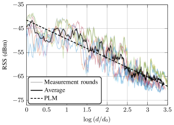
Figure 2: RSS measurements and PLM parameterized by $\hat{\beta}=1.82$.

The data obtained from the measurement rounds contains a total of $L$ RSS measurements at distinct coordinates, which are used for estimating the PLM parameters assuming (2) as model. For this estimation task, least squares (LS) estimation is employed [16].

Ignoring the noise term, (2) can be rewritten in a matrix form as

$$\mathbf{y}=\mathbf{X}\boldsymbol{\theta},$$ (11)

where $\boldsymbol{\theta}=\left[P_{0},\,\beta\right]^{\mathrm{T}}$, $\mathbf{y}=\left[P(\mathbf{d}/d_{0})\right]^{\mathrm{T}}\in\mathbb{R}^{L\times 1}$ contains the RSS measurements in dBm, $\mathbf{X}=\left[\mathbf{1},\,-10\log_{10}(\mathbf{d}/d_{0})\right]\in\mathbb{R}^{L\times 2}$, where $\mathbf{1}$ is an $L$-long all ones vector, and $\mathbf{d}$ contains the $L$ distinct measurement distances. Hence, the parameter vector is obtained as

$$\boldsymbol{\hat{\theta}}=(\mathbf{X}^{\mathrm{T}}\mathbf{X})^{-1}\mathbf{X}^{\mathrm{T}}\mathbf{y},$$ (12)

and the shadowing noise variance is given by

$$\hat{\sigma}^{2}_{\mathrm{dB}}=\frac{1}{L-1}(\mathbf{y}-\mathbf{X}\boldsymbol{\hat{\theta}})^{\mathrm{T}}(\mathbf{y}-\mathbf{X}\boldsymbol{\hat{\theta}}).$$ (13)

Fig. 2 presents the measured RSS at the SU located at (8.39, 0.3) for all 4 rounds. The corresponding averaged RSS and the fitted PLM curves are also shown. The estimated PLM parameters are $\hat{\beta}=1.82$ and $\hat{\sigma}^{2}_{\mathrm{dB}}=11.83$, which agrees with similar measurement campaigns [9, 17, 18].

V-B Localization accuracy

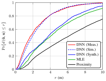
Figure 3: CDF of localization error. Solid lines are obtained from measured data saved exclusively for testing, and the dashed blue line employs synthetic data for testing.

TABLE II: Localization performance statistics

Estimator	Mean LE	SD	Max. LE	Min. LE
DNN (Meas.)	2.3986 m	2.0616 m	11.6976 m	0.0225 m
DNN (Sim.)	2.5153 m	2.0986 m	14.2105 m	0.0151 m
DNN (Synth.)	4.3096 m	3.0279 m	16.7508 m	0.0730 m
MLE	4.8009 m	3.4373 m	17.7379 m	0.3734 m
Proximity	7.0752 m	5.0404 m	37.5100 m	0.5000 m
Localization error (LE), standard deviation (SD)

For assessing the localization performance, we present the cumulative distribution function (CDF) of the localization error, and Table II shows other statistics from the obtained results. The localization error is calculated using (3). Fig. 3 shows the CDF of the localization error for the presented schemes. Solid lines are obtained from measured data saved exclusively for testing consisting of 1174 examples. The dashed line corresponds to the DNN performance when synthetic data is used for training and testing, with the same amount of examples as obtained during the measurement campaign. As we can observe, the performance of DNN (Meas.) and DNN (Sim.) are in agreement. This result suggests that training and analyzing the performance of the DL approach solely with simulated data gives meaningful insight about the expected performance in a real-world scenario. Thus, corroborating the results presented in [6].

Fig. 3 also shows a performance gap between the DNN model obtained from measurements, DNN (Meas.), and the model obtained from synthetic data, DNN (Synth.), when both are tested with measurement data. Several reasons can be attributed to this gap. For instance, the propagation parameters can vary depending on the transmitter position, and this phenomenon is not captured by the PLM employed for synthetic data generation. This non-homogeneity of the indoor propagation channel with respect to different locations has been noted in literature [19]. Moreover, it has been shown that each SU can add a random offset to the RSS measurement due to hardware characteristics [20]. Therefore, it becomes evident that (2) does not capture all effects that characterize the relation between the transmitter position and measured RSS. Another reason is the assumption of an ideal omnidirectional antenna by the PLM, which is often not accurate in practice, since antennas present some level of directivity. These phenomena are captured by the DNN model when trained with measured data, which leads to the improved localization performance when compared with the model trained with synthetic data. The MLE presents similar performance to DNN (Synth.), since both have been designed under the same PLM, and DNNs can be understood as an approximation of MLE [12]. The slight superior performance of DNN (Synth.) over the MLE can be attributed to the quantization error associated with the grid search implementation of the MLE. Moreover, MLE and DNN (Synth.) outperform the Proximity scheme, suggesting that if more accurate propagation models, such as ray tracing, are used for training data generation, the performance of DNN (Synth.) could approach DNN (Meas.).

VI Conclusion

In this paper, we have shown that DL based positioning using data from wireless sensor networks has the potential to be a key technique for providing accurate and reliable position information for improving services in future wireless communications systems. Our experimental investigation suggests that analysing the positioning performance of DL schemes using synthetic data obtained from PLMs gives meaningful predictions of the achievable performance observed in real environments. Furthermore, the potential and downsides of employing synthetic data for training DL models has been discussed. The results suggest that simple PLMs, such as the single slope log-normal, can only provide limited performance, and generating training data through more accurate PLMs is required for reducing the dependency of DL on site-specific measurements.

References

- [1] Federal Communications Commission (FCC), “Wireless E911 location accuracy requirements,” Available at: https://www.federalregister.gov/documents/2020/01/16/2019-28483/wireless-e911-location-accuracy-requirements. Accessed: November 2021.
- [2] H. Viswanathan and P. E. Mogensen, “Communications in the 6G era,” IEEE Access, vol. 8, pp. 57063–57074, 2020.
- [3] C. De Lima, D. Belot, R. Berkvens, A. Bourdoux, D. Dardari, M. Guillaud, M. Isomursu, E.-S. Lohan, Y. Miao, A. N. Barreto, M. R. K. Aziz, J. Saloranta, T. Sanguanpuak, H. Sarieddeen, G. Seco-Granados, J. Suutala, T. Svensson, M. Valkama, B. Van Liempd, and H. Wymeersch, “Convergent communication, sensing and localization in 6g systems: An overview of technologies, opportunities and challenges,” IEEE Access, vol. 9, pp. 26902–26925, 2021.
- [4] O. Kanhere and T. S. Rappaport, “Position location for futuristic cellular communications: 5g and beyond,” IEEE Communications Magazine, vol. 59, no. 1, pp. 70–75, 2021.
- [5] S. A. (Reza) Zekavat, An Introduction to Direction-of-Arrival Estimation Techniques, ch. 9, pp. 303–341. John Wiley & Sons, Ltd, 2018.
- [6] I. B. F. de Almeida, M. Chafii, A. Nimr, and G. Fettweis, “Blind transmitter localization in wireless sensor networks: A deep learning approach,” in 2021 IEEE 32nd Annual International Symposium on Personal, Indoor and Mobile Radio Communications (PIMRC), pp. 1241–1247, 2021.
- [7] I. Bizon, Z. Li, and F. Burmeister, “Indoor received power measurements associated with reference transmitter location using wireless sensor network,” IEEE Dataport, doi: https://dx.doi.org/10.21227/c8ct-gs89, 2022.
- [8] M. Danneberg, R. Bomfin, S. Ehsanfar, A. Nimr, Z. Lin, M. Chafii, and G. Fettweis, “Online wireless lab testbed,” in 2019 IEEE Wireless Communications and Networking Conference Workshop (WCNCW), pp. 1–5, 2019.
- [9] T. Rappaport, Wireless communications: Principles and practice. Prentice Hall communications engineering and emerging technologies series, Prentice Hall, 2nd ed., 2002.
- [10] S. S. Szyszkowicz, H. Yanikomeroglu, and J. S. Thompson, “On the feasibility of wireless shadowing correlation models,” IEEE Transactions on Vehicular Technology, vol. 59, no. 9, pp. 4222–4236, 2010.
- [11] J. Salo, L. Vuokko, H. M. El-Sallabi, and P. Vainikainen, “An additive model as a physical basis for shadow fading,” IEEE Transactions on Vehicular Technology, vol. 56, no. 1, pp. 13–26, 2007.
- [12] I. Goodfellow, Y. Bengio, and A. Courville, Deep Learning. MIT Press, 2016.
- [13] D. P. Kingma and J. Ba, “Adam: A method for stochastic optimization,” arXiv preprint arXiv:1412.6980, 2014.
- [14] X. Glorot and Y. Bengio, “Understanding the difficulty of training deep feedforward neural networks,” in Proceedings of the thirteenth international conference on artificial intelligence and statistics, pp. 249–256, 2010.
- [15] D.-A. Clevert, T. Unterthiner, and S. Hochreiter, “Fast and accurate deep network learning by exponential linear units (elus),” arXiv preprint arXiv:1511.07289, 2015.
- [16] C. Gustafson, T. Abbas, D. Bolin, and F. Tufvesson, “Statistical modeling and estimation of censored pathloss data,” IEEE Wireless Communications Letters, vol. 4, no. 5, pp. 569–572, 2015.
- [17] G. Zanca, F. Zorzi, A. Zanella, and M. Zorzi, “Experimental comparison of rssi-based localization algorithms for indoor wireless sensor networks,” in Proceedings of the Workshop on Real-World Wireless Sensor Networks, REALWSN ’08, (New York, NY, USA), Association for Computing Machinery, 2008.
- [18] J. Miranda, R. Abrishambaf, T. Gomes, P. Gonçalves, J. Cabral, A. Tavares, and J. Monteiro, “Path loss exponent analysis in wireless sensor networks: Experimental evaluation,” in 2013 11th IEEE International Conference on Industrial Informatics (INDIN), pp. 54–58, 2013.
- [19] H. Hashemi, “The indoor radio propagation channel,” Proceedings of the IEEE, vol. 81, no. 7, pp. 943–968, 1993.
- [20] A. Zanella, “Best practice in rss measurements and ranging,” IEEE Communications Surveys Tutorials, vol. 18, no. 4, pp. 2662–2686, 2016.