Blind Transmitter Localization Using Deep Learning: A Scalability Study

Abstract

This work presents an investigation on the scalability of a deep leaning (DL)-based blind transmitter positioning system for addressing the multi transmitter localization (MLT) problem. The proposed approach is able to estimate relative coordinates of non-cooperative active transmitters based solely on received signal strength measurements collected by a wireless sensor network. A performance comparison with two other solutions of the MLT problem are presented for demonstrating the benefits with respect to scalability of the DL approach. Our investigation aims at highlighting the potential of DL to be a key technique that is able to provide a low complexity, accurate and reliable transmitter positioning service for improving future wireless communications systems.

I Introduction

In this paper a deep learning (DL)-based framework that addresses the problem of estimating the relative position of multiple active transmitters within an area of interest using received signal strength (RSS) measurements collected by a wireless sensor network (WSN) as sole position information source is presented. We focus on simultaneous blind transmitter localization, which refers to a functionality that can be implemented at the network side for enabling simultaneous localization of multiple transmitters without prior assumption on the transmission protocol, or propagation characteristics of the environment. Therefore, this approach can be implemented independently of specific wireless standards, and covers a range of different applications, such as localizing interfering nodes within a private wireless network.

Differently from the single transmitter case, where the WSN collects RSS measurements coming from a single source, the RSS obtained at each sensing unit (SU) when multiple transmitters are active is a sum of the transmitted power from different sources. Under this scenario, and assuming the often used log-normal path loss model (PLM) given by (1), the RSS at each SU has the distribution of a sum of log-normals. This random variable does not have a closed-form density function [1]. Hence, model-driven approaches rely on approximations of this distribution for deriving position estimators, e.g., [2]. Moreover, hardware dependent nonlinearities that affect the RSS measurement are not captured by (1). An analysis of hardware related influences on RSS measurement has been presented by A. Zannela in [3] together with guidelines for dealing with the shortcomings stemming from these nonlinearities and propagation effects. As the number of available SUs largely influences the accuracy of the positioning algorithms, it is reasonable to assume that inexpensive SUs with limited hardware capabilities are preferred for implementing a dense WSN. Consequently, the solutions of the multi transmitter localization (MTL) problem that present high localization accuracy also present a high degree of implementation complexity due to the lack of tractable mathematical models. This motivates the adoption of DL as an approach for addressing this problem, since underling hardware-induced nonlinear patterns can be identified from the data collected by the SUs. Similar works on RF-based transmitter identification have shown promising results [4, 5].

More recent and closely related works on DL-based MTL often seek to represent position related information, i.e., RSS, channel state information (CSI), time of arrival (ToA) or angle of arrival (AoA), in formats that resemble the structure of images, so aiming at taking advantage of the well-developed convolutional neural network (CNN) architectures employed in object recognition tasks [6, 7, 8]. In contrast, we argue that a simpler, and consequently less computationally expensive, deep neural network (DNN) architecture already suffices to achieve good generalization performance for the MTL task. In previous works, we proposed a DNN architecture using solely fully connected nodes, and investigated its performance when compared to classical and state-of-the-art approaches [9]. In [10], we employed the proposed scheme to analyze its localization performance when real-world RSS measurements [11] are available, and to understand the achievable real-time performance by employing such technique. The research carried out in previous works now motivates the investigation on the scalability of the DL approach for localization of multiple simultaneous active transmitters.

The proposed approach is divided into two stages. Firstly, the number of active transmitters is estimated using a classification DNN model, and secondly the corresponding transmitters’ coordinates are estimated by a regression DNN model trained for a specific number of active transmitters. Both tasks rely solely on RSS measurements collected by a WSN as input information. The proposed architecture employed for positioning is also used for estimating the number of active transmitters present in the area of interest.

In this work, the proposed approach is compared against two other approaches with different degrees of computational complexity. Namely, (i) radio environment map localization (REML) [12], where an interpolated RSS map of arbitrary pixel resolution is constructed with the measurements collected by the WSN. In the case of a single active transmitter, the position of the active transmitters is then estimated as the pixel coordinate that contains the highest RSS value, whereas for MTL, high power regions are first identified, and the corresponding transmitters’ coordinates are estimated as the center of such regions; (ii) particle simulation (PS), where the localization problem is modeled analogously to a physical particle simulation [13].

The remainder of the paper is organized as follows: Section II presents the mathematical model that characterizes the propagation phenomena. Section III describes the localization algorithms. Section IV presents an analysis of the performance achieved by the localization schemes. Finally, the paper is concluded in Section V.

II System Model

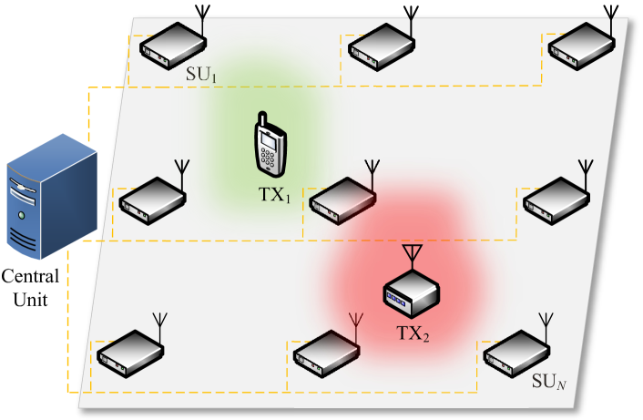
Figure 1: Illustration of a wireless network hosting the DL-based localization service. The RSS measurements are collected by the SUs, which are spatially distributed in grid, and sent to the CU, where the number and the relative coordinates of the active transmitters are estimated using a selection DNN models.

As illustrated in Fig. 1, let us consider that within the area of interest, $N_{s}$ SUs are placed in fixed locations and connected to a CU forming a WSN. The SUs collect RSS measurements in a frequency band for sufficient time to average out small scale fading effects, and send them to a CU, where the number of active transmitters and their corresponding coordinates are estimated.

Let $\mathbf{p}=\left[P_{1},\,\cdots,\,P_{N_{s}}\right]^{\mathrm{T}}$ represent the measurement vector, which contains the RSS values measured by $N_{s}$ SUs, where $P_{j}=10\log_{10}\left(p_{j}\right)$ dBW, and the $j$-th SU measurement in linear scale can be expressed as

$$p_{j}=\sum_{i=1}^{N_{t}}p_{0i}\left(\frac{d\left(\mathbf{u}_{i},\mathbf{v}_{j}\right)}{d_{0}}\right)^{-\beta}w_{ij},$$ (1)

where $N_{t}$ is the total number of active transmitters, $p_{0i}$ is the received power at a reference distance $d_{0}$ from the $i$-th transmitter, $\beta$ represents the path loss exponent, which depends on the environment. $\mathbf{u}_{i}\triangleq\left[u_{i_{x}},u_{i_{y}}\right]^{\mathrm{T}}$ contains the unknown coordinates of the $i$-th transmitter in two dimensions, however, extension to three dimensions is straightforward, $\mathbf{v}_{j}\triangleq\left[v_{j_{x}},v_{j_{y}}\right]^{\mathrm{T}}$ are the coordinates of the $j$-th SU, and $d\left(\mathbf{u}_{i},\mathbf{v}_{j}\right)$ denotes the Euclidean distance between the $i$-th transmitter and $j$-th SU. Lastly, $w_{ij}=10^{n_{ij}/10}$ accounts for the random power fluctuations due to multi-path propagation and random movement, i.e., shadowing noise, where $n_{ij}$ are the entries from a zero-mean Gaussian random vector $\mathbf{n}_{i}$ with covariance matrix $\mathbf{C}\in\mathbb{R}^{N_{s}\times N_{s}}$. The spatial correlation of the shadowing noise is modeled with an exponential decay. Therefore, the entries of $\mathbf{C}$ are a function of the distances among SUs and the decorrelation distance, which is assumed to be in the order of 1 meter for indoor propagation [14].

III Localization Approaches

III-A Deep Learning Based Localization

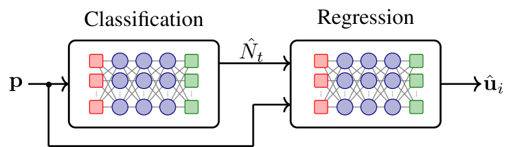
Figure 2: Diagram of the two stage DL-based localization scheme.

Our approach is divided into two steps, and it can be classified as non-cooperative as the transmitters can be simultaneously active. Firstly, the number of active transmitters is estimated. This task can be carried out by different techniques, such as energy detection and cyclostationary feature detection [15, 16, 17]. However, the proposed DNN architecture can also be trained for this classification task with a modification of its last layer, and loss function. Secondly, the estimation of the coordinates is carried out by the DNN architecture selected based on the outcome from the first step, i.e., a particular architecture is used depending on the number of active transmitters to be localized. Note that the only architecture modification needed is a different number of output units, e.g., for localizing two transmitters, the architecture requires four output units for two dimensional positioning, and six units for three dimensions. Both tasks can be modeled as supervised learning problems, given a data set with transmitters coordinates, or number of active transmitters, and associated RSS measurements. The approach is illustrated in Fig. 2.

The DNN architecture employed in this paper has been proposed in our previous work [9], where we draw inspiration from the well-investigated log-normal PLM that associates RSS to the transmitter-receiver separation distance as a starting point for selecting the architecture. This led to a fully connected DNN, where the number of hidden layers is chosen based on the number of nonlinear functions between the transmitter position and the corresponding RSS measurements. Observing (1), there is a two-fold nonlinear functional relation between the transmitters coordinates and RSS measurements. Moreover, taking into account the nonlinear effects induced by the hardware, an architecture with 3 hidden layers was selected. It is worth noting that, a single hidden layer architecture is capable of approximating any function given a sufficiently large number of hidden units [18]. However, successful practical examples of DL algorithms suggest that architectures with multiple hidden layers are able to approximate complex functions with significant less hidden units [19].

Differently from [9], the exponential linear unit (ELU) is chosen as activation function instead of the rectified linear unit (ReLU), since its output does not produces zero for negative inputs, and thus deactivating neurons. Furthermore, its gradient is continuous, and according to our most recent experiments ELU performs slightly better than ReLU w.r.t. localization accuracy. The hyper-parameters of the selected architecture are presented in Table I.

TABLE I: DNN hyperparameters.

Hyperarameter	Value
Number of hidden layers	3
Number of hidden units per layer	128
Validation split	80% training, 20% validation
Mini batch size	40
Regularization parameter (L2)	0.01
Activation function of hidden units	ELU
Optimizer	Adaptive moments (Adam)
Learning rate	10-4
Loss function	mean squared error (MSE)
Weight initialization	Xavier

For obtaining the transmitters’ coordinates, the last layer has a linear activation function, and its number of units depends upon the number of simultaneous active transmitters, i.e., twice the number of transmitters for two dimensional positioning.

An ambiguity problem arises depending on how the data set for training is organized. To illustrate this problem, let us assume the presence of two transmitters, the same measurement vector can be obtained when $\mathbf{u}=\left[u_{1_{x}},u_{1_{y}},u_{2_{x}},u_{2_{y}}\right]$ and when $\mathbf{u}=\left[u_{2_{x}},u_{2_{y}},u_{1_{x}},u_{1_{y}}\right]$. To avoid such problem in the data set creation, the transmitter coordinates are ordered such that transmitters with smaller indices have the smaller coordinate values for a given example. In other words, the known coordinates are arranged such that $u_{i_{x}},u_{i_{y}}<u_{(i+1)_{x}},u_{(i+1)_{y}}$. Note that this does not pose a constraint on the functionality of the proposed solution, since distinguishing individual transmitters’ indexes might not be of interest for practical applications, such as unauthorized transmitter localization.

The online computational complexity is represented by the number of real multiplications required by the DNN estimator, and it can be written w.r.t. the network architecture as

$$\mathcal{C}_{\mathrm{DNN}}=\sum_{l=1}^{L-1}\left(N_{u}^{(l-1)}+1\right)N_{u}^{(l)},$$ (2)

where $N_{u}^{(l)}$ represents the number of units in the $l$-th layer of the network, $L$ is the total number of layers including input and output layers.

III-B Radio Environment Map Localization (REML)

This localization approach divides the area of interest into discrete regions with resolution $R$ meters, and it uses an estimated REM for obtaining the transmitters coordinates [12]. The REM is acquired via ordinary Kriging interpolation, where the RSS predictions at arbitrary pixel points are estimated based on the second order statistics of the measured RSS [20]. The resulting REM contains the estimated RSS values for all pixels in the area using RSS measurements for the pixels that contain the SUs.

Let $P_{w}=A_{w}/R$ and $P_{h}=A_{h}/R$ represent the total number of pixels along the width and height of the area, where $A_{w}$ and $A_{h}$ are the width and height in meters, respectively. The total number of pixels within the area is $K=P_{w}\times P_{h}$ pixels. For avoiding RSS variation within one pixel, $R$ has to be greater than the decorrelation distance. The REM is then stored in a matrix $\mathbf{U}\in\mathbb{R}^{P_{w}\times P_{h}}$. Assuming a single transmitter, the pixel coordinates are estimated by selecting the element which contains the highest RSS value as

$$\mathbf{\hat{u}}_{\mathrm{pixel}}=\underset{i,j}{\arg\max}\left[\mathbf{U}\right]_{i,j},$$ (3)

where the continuous space coordinates are obtained by $\mathbf{\hat{u}}_{\mathrm{REML}}=\mathbf{\hat{u}}_{\mathrm{pixel}}/R$. For the case of multiple transmitters, histogram thresholding and image segmentation need to be applied to $\mathbf{U}$ for distinguishing regions with significant RSS. After this procedure, the transmitters pixel coordinates are estimated as the pixel with highest RSS within each region. It is worth noting that REML does not require previous knowledge on the transmit power or number of active transmitters, making it also practical for blind localization. The REML computational complexity is given by

$$\mathcal{C}_{\mathrm{REML}}=KN_{s}\log(N_{s}).$$ (4)

III-C Particle Simulation

This localization method is based on a particle simulation. Therefore, all SUs and active transmitters are assumed to be particles. The SUs are fixed and initialized at their corresponding known positions. In contrast, the transmitters are initialized close to the SUs with the strongest RSS measurements, and they can move freely during the algorithm iterations. Initially, the RSS will be calculated for each SU based on their current positions and the PLM. Since the initial transmitter positions differ from the true positions, and there are other influences such as shadowing, the calculated RSS will differ from the measured RSS at the SUs. These errors are interpreted as potentials that will imply some forces onto the particles. Hence, the SUs that have measured more than calculated become attractors, whereas the others will become repellers. The forces induce movement on the free particles, i.e., transmitters, such that they will iteratively move closer to the best position that matches the measured RSS. Note that in this scheme, the transmit power is assumed to be known in advance. More details may be found in [13].

The algorithm iterations stop, if one of the following conditions is met: (i) the number of iterations exceeds $N_{\mathrm{iter}}=500$, (ii) the total movement of the particles is smaller than 10^-3 meters, or (iii) the Euclidian norm of the vector of errors in receive powers is smaller than 10^-2 dB. The computational complexity is dominated by the PLM calculation for each pair of transmitter and SU that is required to obtain the forces that affect particles in each iteration. Hence, the computational complexity is given by the product

$$\mathcal{C}_{\mathrm{PS}}=N_{s}N_{t}N_{\mathrm{iter}}$$ (5)

IV Simulation Results Regarding Scalability

The performance shown in this section focuses on the scalability of the DL approach with respect to sensor density, and number of simultaneous active transmitters. As localization performance metric, we present the cumulative distribution function (CDF) of the localization error, where this error is defined as the Euclidean distance between the true position and the estimated one. For comparison we tested the data with the approaches in [13], and in [12]. For the sake of comparison with the more sophisticated techniques, the performance obtained with random guess (RG) is also presented as an upper bound for the positioning error. In this case, the transmitters’ coordinates are estimated by drawing realizations from a uniform distribution ranging between 0 and the area limits.

The data sets used are obtained following the model described by (1). The path loss exponent is fixed to $\beta=3.23$, which corresponds to an indoor space with relatively high signal attenuation [21]. A maximum of four simultaneous transmitters coexist in the area. This quantity is assumed to be known a priori for Fig. 4, and it is used for selecting the required DNN architecture for localization. Therefore, one DNN model is trained for each $N_{t}$. The coordinates of the transmitters at each example are generated through an uniform distribution between zero and the area limits. The shadowing noise variance of the training and test data sets is fixed and equal to 10 dB. Note that for training and testing, independent data sets were generated. All relevant simulation parameters are shown in Table II.

TABLE II: Simulation parameters.

Parameter	Value
Fixed transmit power	20 dBm
Antenna radiation pattern	Omnidirectional
Path loss exponent ($\beta$)	3.23
Shadowing noise variance	$\sigma^{2}_{\mathrm{dB}}=10$
Decorrelation distance	1 meter
Area size	20 $\times$ 20 m2
Number of SUs	16 (Figs. 3, 4, 5)
Sensor density	4 sensor/100 m2 (Figs. 3, 4, 5)
Number of active transmitters ($N_{t}$)	1, 2, 3 and 4
SU arrangement	Grid
Frequency of operation	2.4 GHz
REML pixel resolution	10 cm
PS maximum number of iterations	500
Number of training examples	3000 per active transmitter
Number of testing examples	3000 per active transmitter
Number of training epochs	1000

IV-A Multiple Active Transmitters

IV-A1 Classification Performance

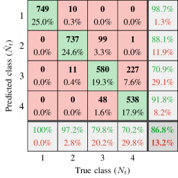
Figure 3: Confusion matrix.

Fig. 3 illustrates the classification performance of the DNN model assuming up to four simultaneously active transmitters. The rightmost column of the confusion matrix displays the precision of the model, whereas the row in the bottom presents the recall values, and the element at the bottom right displays the model’s overall accuracy. As the number of active transmitters increases, the classification performance decreases. Nevertheless, precision and recall values do not fall below 70% for the total of 3000 examples tested.

IV-A2 Localization Performance

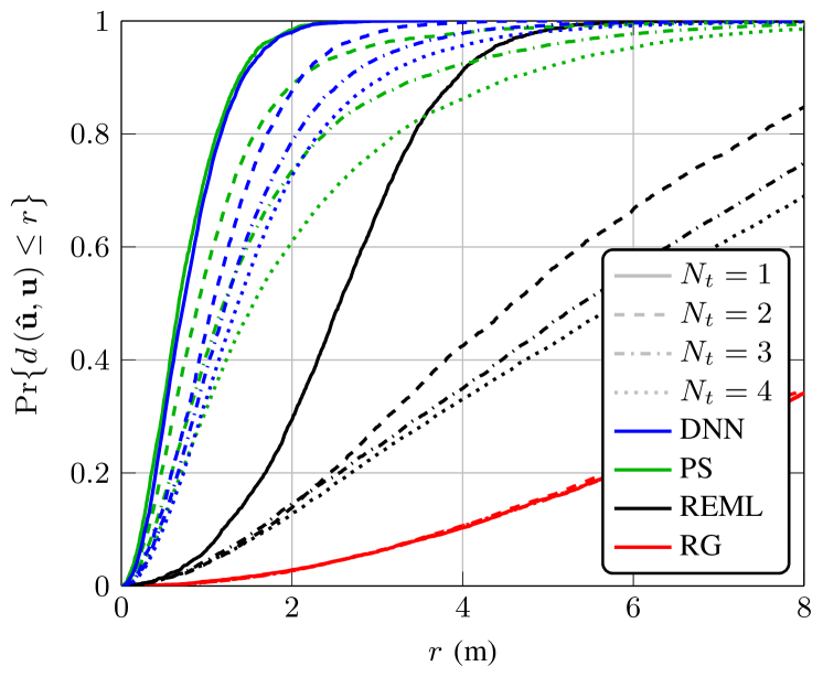
Figure 4: CDF of the positioning error with a varying number of simultaneously active transmitters for the DL, PS and REML algorithms.

Fig. 4 shows the localization performance of the algorithms assuming up to four simultaneous transmitters. The DL approach yields sub 4 meter accuracy for all data tested, with performance degradation as the number of active transmitters increases. In Fig. 4, one DNN model was obtained for each number of simultaneously active transmitters. The REML shows acceptable performance only for $N_{t}<2$. For $N_{t}\geq 2$, the likelihood that two transmitters are close enough such that the regions of high RSS levels cannot be distinguished is significant, and the localization accuracy reduces for this reason. The PS method shows similar performance when compared to DL for $N_{t}\leq 2$. However, PS presents slight localization performance degradation as the number of transmitters increases.

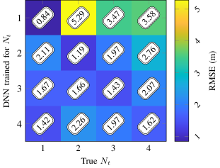
Figure 5: RMSE matrix of the estimated coordinates when $N_{t}$ is misclassified.

Fig. 5 illustrates the root mean squared error (RMSE) matrix of the estimated coordinates when $N_{t}$ is misclassified. The RMSE is obtained by using the closest coordinates when $N_{t}$ is misclassified. As it can be observed the largest positioning errors occur when there are more active transmitters than what was obtained in the classification stage, i.e, a model trained for a larger $N_{t}$ performs better than a model trained for smaller $N_{t}$ in a misclassification scenario. This result resonates with the idea that a DNN model can only perform well when it is exposed to data that it is similar to the data contained within the training set. Correspondingly, the model trained for $N_{t}=4$ performs better than the model trained for $N_{t}=1$ when $N_{t}$ is misclassified. Furthermore, a joint analysis of Figs. 3 and 5 shows that when misclassification errors are more likely, i.e., larger $N_{t}$, the average positioning error is less degraded.

IV-B Sensor Density

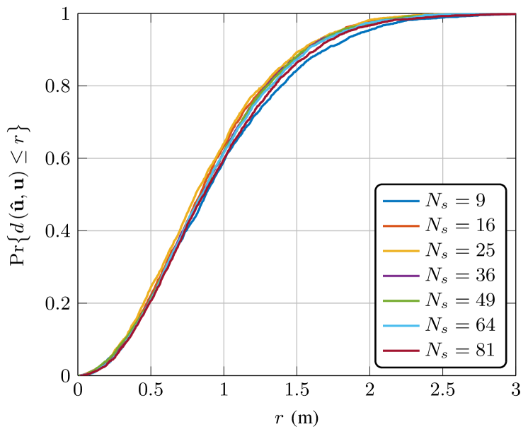
Figure 6: CDF of the positioning error assuming a constant sensor density of 4 sensor/100 m² and $N_{t}=1$ for the DL approach.

Fig. 6 shows the localization performance of the DL approach for the single transmitter case assuming a constant sensor density, i.e., as $N_{s}$ increases the area size increases proportionally in order to keep the ratio $(A_{w}\times A_{h})/N_{s}$ constant. As can be observed, the resulting localization performance remains also constant. This result indicates that the localization performance observed in a specific scenario, i.e., area size and $N_{s}$, can be extrapolated to a more general setting.

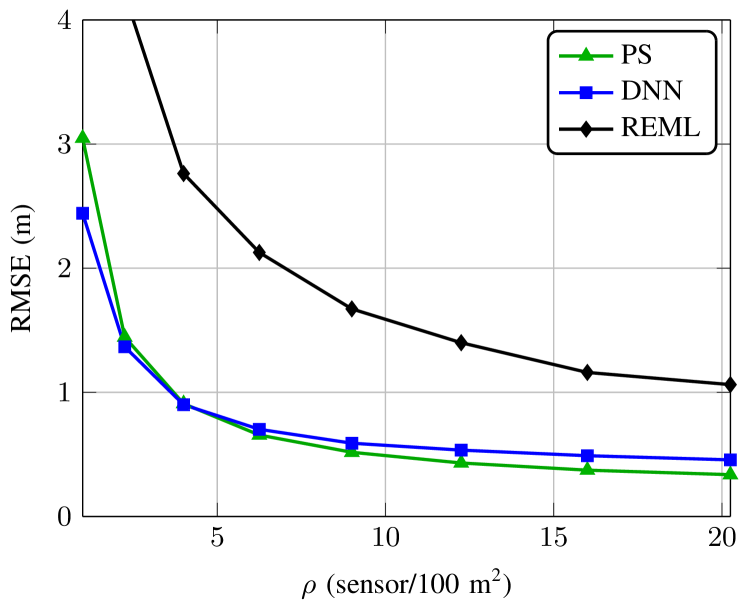
Figure 7: RMSE of the estimated coordinates versus SU density assuming a constant area of 20 by 20 m² and $N_{t}=1$ for the DL, PS and REML approaches.

Fig. 7 presents the localization accuracy averaged over several positions across the area as a function of the SU density in sensor/100 m². Unsurprisingly, lower SU density leads to lower localization accuracy for all localization algorithms. Moreover, in the lower SU density DNN performs slightly better than PS, this results can be attributed to the limited number of iterations used in the particle simulation. In the higher SU density regime, PS outperforms DNN also by a small margin, since PS requires the extra apriori information about the transmit power. Furthermore, for all algorithms the gain in accuracy is relatively low for $\rho>15$ sensor/100 m², which when compared to the cost increase in SUs installation, suggests that no significant improvement on localization performance can be obtained at the expense of increasing SU density.

V Conclusion

In this paper, the performance of a low complexity DL-based localization framework has been investigated for positioning multiple transmitters in indoor scenarios. The observed simulation results indicate that this approach is able to address the challenging MTL problem, and its localization performance scales well with an increasing number of active transmitters. Furthermore, it has been observed that evaluating the localization performance with respect to SU density in scaling environments with similar characteristics is sufficient to gather insights on the expected positioning accuracy. Nevertheless, the localization performance saturates after a certain SU density. This observation suggests that more input information rather than exclusively RSS measurements is required for achieving sub-meter localization accuracies.

References

- [1] S. C. Schwartz and Y. S. Yeh, “On the distribution function and moments of power sums with log-normal components,” Bell System Technical Journal, vol. 61, no. 7, pp. 1441–1462, 1982.
- [2] J. K. Nelson, M. R. Gupta, J. E. Almodovar, and W. H. Mortensen, “A quasi em method for estimating multiple transmitter locations,” IEEE Signal Processing Letters, vol. 16, no. 5, pp. 354–357, 2009.
- [3] A. Zanella, “Best practice in rss measurements and ranging,” IEEE Communications Surveys Tutorials, vol. 18, no. 4, pp. 2662–2686, 2016.
- [4] C. Morin, D. Duchemin, J.-M. S. Gorce, C. Goursaud, and L. Sampaio Cardoso, “Active user blind detection through deep learning,” in Crowncom 2020 - 15th EAI International Conference on Cognitive Radio Oriented Wireless Networks, (Rome, Italy), pp. 1–14, Nov. 2020.
- [5] O. Omotere, J. Fuller, L. Qian, and Z. Han, “Spectrum occupancy prediction in coexisting wireless systems using deep learning,” in 2018 IEEE 88th Vehicular Technology Conference (VTC-Fall), pp. 1–7, 2018.
- [6] A. Zubow, S. Bayhan, P. Gawłowicz, and F. Dressler, “Deeptxfinder: Multiple transmitter localization by deep learning in crowdsourced spectrum sensing,” in 2020 29th International Conference on Computer Communications and Networks (ICCCN), pp. 1–8, 2020.
- [7] C. Zhan, M. Ghaderibaneh, P. Sahu, and H. Gupta, “Deepmtl: Deep learning based multiple transmitter localization,” in 2021 IEEE 22nd International Symposium on a World of Wireless, Mobile and Multimedia Networks (WoWMoM), pp. 41–50, 2021.
- [8] F. Mitchell, A. Baset, N. Patwari, S. K. Kasera, and A. Bhaskara, “Deep learning-based localization in limited data regimes,” in Proceedings of the 2022 ACM Workshop on Wireless Security and Machine Learning, WiseML ’22, (New York, NY, USA), pp. 15–20, Association for Computing Machinery, 2022.
- [9] I. B. F. de Almeida, M. Chafii, A. Nimr, and G. Fettweis, “Blind transmitter localization in wireless sensor networks: A deep learning approach,” in 2021 IEEE 32nd Annual International Symposium on Personal, Indoor and Mobile Radio Communications (PIMRC), pp. 1241–1247, 2021.
- [10] I. Bizon, Z. Li, A. Nimr, M. Chafii, and G. P. Fettweis, “Experimental performance of blind position estimation using deep learning,” in 2022 IEEE Global Communications Conference: Selected Areas in Communications: Machine Learning for Communications (Globecom2022 SAC MLC), (Rio de Janeiro, Brazil), Dec. 2022.
- [11] I. Bizon, Z. Li, and F. Burmeister, “Indoor received power measurements associated with reference transmitter location using wireless sensor network,” IEEE Dataport, doi: https://dx.doi.org/10.21227/c8ct-gs89, 2022.
- [12] K. Kulkarni, N. Franchi, and G. Fettweis, “Real-time cooperative spectrum sensing: Reliable localization of unknown interferers in shared spectrum,” in SCC 2019; 12th International ITG Conference on Systems, Communications and Coding, pp. 1–6, 2019.
- [13] P. Schulz, N. Franchi, and G. Fettweis, “Rss-based localization of multiple unknown transmitters through particle simulation,” in 2021 1st IEEE International Online Symposium on Joint Communications & Sensing (JC&S), pp. 01–06, 2021.
- [14] J. Salo, L. Vuokko, H. M. El-Sallabi, and P. Vainikainen, “An additive model as a physical basis for shadow fading,” IEEE Transactions on Vehicular Technology, vol. 56, no. 1, pp. 13–26, 2007.
- [15] H. Li, X. Wang, and Y. Zou, “Exploiting transmitter I/Q imbalance for estimating the number of active users,” in 2013 IEEE Global Communications Conference (GLOBECOM), pp. 3318–3322, 2013.
- [16] M. Zheleva, R. Chandra, A. Chowdhery, A. Kapoor, and P. Garnett, “Txminer: Identifying transmitters in real-world spectrum measurements,” in 2015 IEEE International Symposium on Dynamic Spectrum Access Networks (DySPAN), pp. 94–105, 2015.
- [17] G. Ding, J. Yuan, J. Bao, and G. Yu, “LSTM-based active user number estimation and prediction for cellular systems,” IEEE Wireless Communications Letters, vol. 9, no. 8, pp. 1258–1262, 2020.
- [18] A. Kratsios, “The universal approximation property. characterization, construction, representation, and existence,” Annals of Mathematics and Artificial Intelligence, pp. 435–469, Jan 2021.
- [19] I. Goodfellow, Y. Bengio, and A. Courville, Deep Learning. MIT Press, 2016.
- [20] D. Mao, W. Shao, Z. Qian, H. Xue, X. Lu, and H. Wu, “Constructing accurate radio environment maps with kriging interpolation in cognitive radio networks,” in 2018 Cross Strait Quad-Regional Radio Science and Wireless Technology Conference (CSQRWC), pp. 1–3, 2018.
- [21] J. Miranda, R. Abrishambaf, T. Gomes, P. Gonçalves, J. Cabral, A. Tavares, and J. Monteiro, “Path loss exponent analysis in wireless sensor networks: Experimental evaluation,” in 2013 11th IEEE International Conference on Industrial Informatics (INDIN), pp. 54–58, 2013.