Relativistic phase space diffusion of compact object binaries
in stellar clusters and hierarchical triples

Abstract

The LIGO/Virgo detections of compact object mergers have posed a challenge for theories of binary evolution and coalescence. One promising avenue for producing mergers dynamically is through secular eccentricity oscillations driven by an external perturber, be it a tertiary companion (as in the Lidov-Kozai (LK) mechanism) or the tidal field of the stellar cluster in which the binary orbits. The simplest theoretical models of these oscillations use a ‘doubly-averaged’ (DA) approximation, averaging both over the binary’s internal Keplerian orbit and its ‘outer’ barycentric orbit relative to the perturber. However, DA theories do not account for fluctuations of the perturbing torque on the outer orbital timescale, which are known to increase a binary’s eccentricity beyond the maximum DA value, potentially accelerating mergers. Here we reconsider the impact of these short-timescale fluctuations in the test-particle quadrupolar limit for binaries perturbed by arbitrary spherical cluster potentials (including LK as a special case), in particular including 1pN general relativistic (GR) apsidal precession of the internal orbit. Focusing on the behavior of the binary orbital elements around peak eccentricity, we discover a new effect, relativistic phase space diffusion (RPSD), in which a binary can jump to a completely new dynamical trajectory on an outer orbital timescale, violating the approximate conservation of DA integrals of motion. RPSD arises from an interplay between secular behavior at extremely high eccentricity, short-timescale fluctuations, and rapid GR precession, and can change the subsequent secular evolution dramatically. This effect occurs even in hierarchical triples, but has not been uncovered until now.

1. Introduction

The compact object — black hole (BH) and/or neutron star (NS) — binary mergers discovered by the LIGO/Virgo collaboration in recent years (Abbott et al., 2021) have reinvigorated the detailed study of secular evolution of binaries in external tidal fields. The most famous scenario of this kind is a hierarchical triple, in which the compact object binary in question is orbited by a bound tertiary companion. In this case the tertiary companion can drive secular oscillations of the binary orbital elements — known as Lidov-Kozai (LK) oscillations (Lidov, 1962; Kozai, 1962) — on timescales much longer than either orbital period. Alternatively, very similar secular evolution arises if one considers a binary perturbed not by a tertiary point mass but by the global tidal field of the stellar cluster in which it resides (Hamilton & Rafikov, 2019b, c, a; Bub & Petrovich, 2020). In either scenario, the key idea is that secular tidal forcing can increase a binary’s eccentricity dramatically. Provided this forcing is strong enough to overcome 1pN general relativistic (GR) apsidal precession — which acts to decrease the maximum eccentricity (Wen, 2003; Hamilton & Rafikov, 2021) — the binary can thereby achieve a small pericenter distance, allowing it to radiate gravitational waves (GWs) efficiently and thus rapidly merge. Similar mechanisms have been invoked to explain the origin of other exotic objects, such as Type 1a supernovae (Katz & Dong, 2012), blue stragglers (Leigh et al., 2018), hot Jupiters (Fabrycky & Tremaine, 2007), and so on.

Regardless of the particular system under consideration, the same two key questions always arise: (i) under what circumstances can a binary reach extremely high eccentricity on an astrophysically relevant timescale? and (ii) how does the binary behave when it reaches such extreme eccentricities?

Question (i) is straightforward to answer using secular theories, the simplest of which involve truncating the perturbing potential at quadrupole order, taking the ‘test particle’ approximation and then ‘double-averaging’ (DA) — that is, averaging the dynamics over both the binary’s ‘inner’ Keplerian orbit and over its ’outer’ barycentric motion relative to the perturbing potential. In Hamilton & Rafikov (2019b, c, 2021) — hereafter Papers I, II and III respectively — we developed the most comprehensive such DA theory to date, capable of describing the secular evolution of any binary perturbed by any fixed axisymmetric potential (in the test particle, quadrupole limit), accounting for 1pN GR precession of the inner orbit. In this theory, which includes the LK scenario as a special case, the binary’s maximum eccentricity $e_{\mathrm{max}}$ can be calculated (semi-)analytically as a function of the initial conditions. As a result one can easily determine the region of parameter space that leads to extremely high $e_{\mathrm{max}}$. In the case of spherical cluster potentials (including the Keplerian LK case) which we will focus on exclusively throughout this paper, one always finds that $e_{\mathrm{max}}$ is limited by the initial relative inclination $i_{0}$ between the binary’s inner and outer orbital planes:

$$e_{\mathrm{max}}\leq e_{\mathrm{lim}}\equiv(1-\Theta)^{1/2},$$ (1)

where

$$\Theta\equiv(1-e_{0}^{2})\cos^{2}i_{0},$$ (2)

and $e_{0}$ is the initial eccentricity. Hence, a necessary (but not always sufficient) part of the answer to question (i) is that $\Theta\ll 1$.

However, DA theories often do not provide an accurate answer to question (ii). That is because DA theory ignores a component of the torque that fluctuates on the timescale of the outer orbit, and normally washes out to zero upon averaging over that timescale. This becomes problematic at extremely high eccentricity, when the relative changes in the binary’s (very small) angular momentum due to this fluctuating torque can become $\mathcal{O}{(1)}$. As a result, the DA theory can fail to capture the dynamics in detail. A more accurate (if more cumbersome) description is provided by the singly-averaged (SA) theory, in which one only averages over the binary’s inner Keplerian orbit, and hence captures fully the fluctuations in the orbital elements on the outer orbital timescale. In particular, these short-timescale fluctuations (sometimes called ‘SA fluctuations’) can increase a binary’s maximum eccentricity beyond $e_{\mathrm{max}}$ (Ivanov et al., 2005). Because of this they can be of great significance when predicting LK-driven merger rates of black hole (BH) or neutron star (NS) binaries, blue straggler formation rates, white dwarf collision rates, and so on (e.g. Katz & Dong 2012; Antonini & Perets 2012; Bode & Wegg 2014; Antonini et al. 2014; Antognini et al. 2014; Luo et al. 2016; Grishin et al. 2018; Lei et al. 2018; Lei 2019; Mangipudi et al. 2022).

Faced with this assessment, one might decide simply to abandon DA theory altogether and only work with the SA equations of motion (e.g. Bub & Petrovich 2020). Alternatively one might choose to forego all averaging, and instead to integrate the ‘N-body’ equations of motion directly (see e.g. the 3-body integration results of Antonini et al. 2014). There are three main objections to these approaches. First, numerical integration of the SA or direct N-body equations is prohibitively expensive if one wants to evolve millions of binary initial conditions, as done in e.g. Hamilton & Rafikov (2019a). Second, SA and N-body approaches necessarily demand more initial data, inflating the parameter space. Third, whatever one gains though brute-force computation, one also often sacrifices in terms of analytical and physical insight. Instead, our approach will be to understand the SA, at high eccentricity in an approximate analytical fashion, guided by the DA theory and by numerical integrations where appropriate. We will restrict ourselves to studying the test particle quadrupole limit, and we will include GR precession of the inner orbit but we will ignore GW emission (though see Hamilton & Rafikov 2022).

In particular, by examining in detail the numerical solutions to the SA equations of motion, we have encountered an important phenomenon which we call relativistic phase space diffusion (RPSD). This phenomenon must have been present in many authors’ direct numerical integrations of the LK problem, but seems not to have been discussed explicitly in the past. The only exception we know of is the recent study by Rasskazov & Rafikov (2023), who confirmed our results numerically, and who extended them by showing that RPSD is present and important even when GW emission is included.

Since RPSD is the key result of this paper, let us now motivate our study with an example of it.

1.1. Example of relativistic phase space diffusion

It is well known that when a binary is driven secularly to very high eccentricity, then even in the DA approximation, its orbital elements (i.e. its eccentricity, argument of pericenter, and longitude of ascending node) exhibit $\mathcal{O}(1)$ fractional changes on the timescale (see Paper III):

$$t_{\mathrm{min}}\sim j_{\mathrm{min}}t_{\mathrm{sec}},$$ (3)

where $j_{\mathrm{min}}\equiv(1-e_{\mathrm{max}}^{2})^{1/2}$ is the minimum dimensionless angular momentum, $e_{\mathrm{max}}$ is the maximum eccentricity, and $t_{\mathrm{sec}}$ is the secular timescale. Clearly, for very large eccentricities, $t_{\mathrm{min}}\ll t_{\mathrm{sec}}$. The central result of this paper is that in the SA approximation, if $t_{\mathrm{min}}$ is so short as to be comparable to or smaller than the outer orbital period $T_{\phi}$, and GR apsidal precession is included, then the binary can very quickly ‘jump’ to a new phase space orbit, such that the DA approximation would fail completely to track the next secular cycle. Said differently, RPSD drives abrupt shifts of the binary’s approximate DA integrals of motion, just like GW emission or stellar encounters could, but in their absence.

To illustrate the RPSD phenomenon, we present Figures 1 and 2. To create these Figures we considered a NS-NS binary with semimajor axis $a=50$ AU, orbiting in (and tidally perturbed by) a spherical Hernquist potential of mass $\mathcal{M}=10^{7}M_{\odot}$ and radial scale $b=1$ pc, which constitutes a simple model of a nuclear stellar cluster. The outer orbit’s azimuthal period is $T_{\phi}=0.064$ Myr. (The full set of initial conditions used here will be described in §3.1.1 after we have introduced our notation more fully). In each Figure, we integrate the (test-particle, quadrupole) SA equations of motion for roughly one secular period $t_{\mathrm{sec}}$. We ran this integration seven times, each time with identical initial conditions except that we give the binary’s outer orbit a different initial radial phase. We also integrated the DA equations of motion for the same initial conditions (in the DA case the outer orbital phase information is irrelevant, since we have averaged over the outer motion). The only difference between Figures 1 and 2 is that in Figure 2, we switched on the effect of 1pN GR apsidal precession. This is a weak effect which only becomes important at very high eccentricity (the dimensionless strength of GR here is $\epsilon_{\mathrm{GR}}\sim 10^{-3}$ — see §2.2.1). We repeat that we do not include GW emission in any of our calculations in this paper.

In both Figures we plot the SA eccentricity, $\log_{10}(1-e)$, for each run (different colored lines) at three stages of the evolution: (a) the very earliest stages near $t=0$, (b) around the eccentricity peak, and (c) the latest stages near $t=t_{\mathrm{sec}}$. The thick dashed blue line in each panel is the DA solution. In Figure 1, we see that although the different SA realizations track each other very closely (at least in log space) in panel (a), around the eccentricity peak in panel (b) they differ quite considerably. Some runs do not even reach the DA maximum eccentricity $\log_{10}(1-e_{\mathrm{max}})\approx-4.75$, while some runs achieve an extremely high eccentricity, $\log_{10}(1-e_{\mathrm{max}})\approx-5.65$. These SA fluctuations at high-$e$ can have a major effect on merger timescales, as is well known (Grishin et al., 2018; Mangipudi et al., 2022). Nevertheless, upon emerging from the eccentricity peak, the different runs converge together (see panel (c)), closely tracking the ‘underlying’ DA solution.

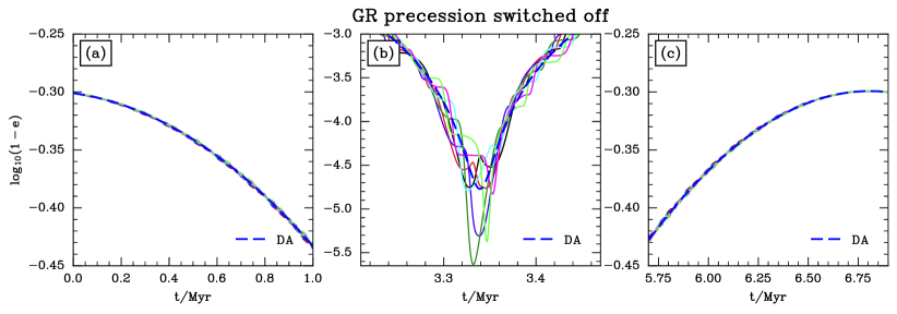
Figure 1.— Example of eccentricity evolution for a NS-NS binary orbiting a Hernquist potential with outer azimuthal period $T_{\phi}=0.064$ Myr, for seven different values of the outer orbit’s initial radial phase. Panels (a) and (c) show the beginning ($t\approx 0$) and end ($t\approx t_{\mathrm{sec}}$) of the calculation, respectively, while panel (b) focuses on the eccentricity peak around $t\approx t_{\mathrm{sec}}/2$. The DA solution (independent of radial phase) is shown with a blue dashed line.

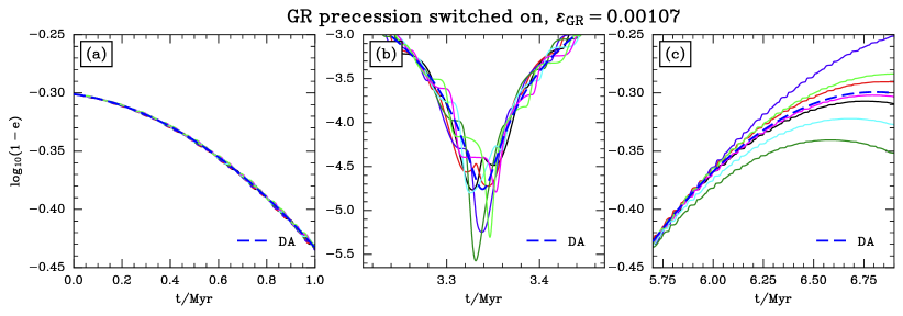
Figure 2.— As in Figure 1, except with 1pN GR apsidal precession switched on. The fact that the trajectories have diverged by $t\sim t_{\mathrm{sec}}$ is a manifestation of relativistic phase space diffusion (RPSD), which is the central result of this paper.

Now we compare this with Figure 2. The early evolution (compare Figures 1a and 2a) is essentially identical with and without GR, as expected away from high-$e$. Next, comparing Figures 1b and 2b, we see that the maximum eccentricity reached by a given binary is very slightly diminished by the inclusion of GR (the green line now reaches $1-e_{\mathrm{max}}\approx-5.6$ rather than $-5.65$), as we would expect given that the binary resides in the weak GR regime (Paper III), but otherwise the evolution is almost indistinguishable from the case without GR. However, by the time the DA eccentricity has returned to its minimum around $6.8$ Myr (panel (c)) most of the SA trajectories have diverged significantly both from the DA solution and from each other. They will subsequently follow entirely different secular evolutionary tracks, many of which will be badly approximated by the original DA solution.

As we will see in §4, over the course of many secular cycles this trajectory divergence results in a ‘diffusion’ of the value of the DA Hamiltonian, which is an approximate integral of motion around which each SA solution would normally fluctuate (as in Figure 1), and will be defined properly in §2. This diffusion behavior breaks down at sufficiently high eccentricity provided GR is switched on, so we call it RPSD. However, by using the term ‘diffusion’ we do not mean to suggest that the system’s integrals of motion follow any simple Brownian walk or that their evolution can be described by a diffusion equation. In fact, the ‘diffusion’ we have found does not seem to obey any simple statistical behavior, as we will see in §4.2.3.

We note here that Luo et al. (2016) also found that short-timescale fluctuations can cause the mean trajectory of a binary to drift gradually away from the DA prediction, even in the test-particle quadrupole LK problem, and derived a ‘corrected DA Hamiltonian’ to account for this deviation. However, this effect is distinct from RPSD, for several reasons: (i) it has nothing to do with GR precession; (ii) it does not require extremely high eccentricity behavior, and (iii) it occurs due to an accumulation of nonlinear quadrupolar perturbations, which are normally averaged out in the standard LK theory, over many secular periods (see Tremaine 2023; these nonlinear effects are too small to be discernible in Figure 1). On the contrary, RPSD only occurs when GR is included, and happens on a much shorter timescale, requiring just one (very high) eccentricity peak. We discuss this comparison further in §5.4.

1.2. Plan for the rest of this paper

The rest of this paper is structured as follows. In §2 we briefly recap some key results from Papers I-III and establish our notation. In §3 we provide several numerical examples that illustrate the phenomenology of short-timescale fluctuations when GR is not included, particularly with regard to high eccentricity behavior. We then proceed to explain the observed behavior quantitatively, and derive an approximate expression for the magnitude of angular momentum fluctuations at high $e$. In §4 we switch on GR precession and give several numerical examples of systems exhibiting RPSD. We then analyse this phenomenon more quantitatively and offer a physical explanation for it. In §5 we consider the astrophysical importance of RPSD, and discuss our results in the context of the existing LK literature. We summarise in §6.

2. Dynamical framework

In this section we recap the basic formalism for describing a binary perturbed by quadrupole-order tides, including 1pN GR precession. For more details see Papers I-III.

2.1. Inner and outer orbits

Consider a binary with component masses $m_{1}$ and $m_{2}$, inside some spherically symmetric host system (the ‘cluster’) whose potential is $\Phi(\mathbf{R})$. The binary’s barycentre $\mathbf{R}_{\mathrm{g}}(t)$ is assumed to move as a test particle in this potential: we call this the ‘outer orbit’. Meanwhile, the binary’s internal Keplerian orbital motion (the ‘inner’ orbit) is described by orbital elements: semi-major axis $a$, eccentricity $e$, inclination $i$, longitude of the ascending node $\Omega$, argument of pericenter $\omega$, and mean anomaly $M$, defined as in Paper I.

An alternative description of this inner orbit is provided by the Delaunay actions $\mathbf{I}=(L,J,J_{z})$, with $L=\sqrt{G(m_{1}+m_{2})a}$, $J=L\sqrt{1-e^{2}}$, and $J_{z}=J\cos i$, and their conjugate angles $\bm{\psi}=(M,\omega,\Omega)$. Sometimes we will find it useful to refer to the dimensionless versions of these variables:

$$j \equiv J/L=(1-e^{2})^{1/2},$$ (4)

$$j_{z} \equiv J_{z}/L=(1-e^{2})^{1/2}\cos i,$$ (5)

$$\Theta \equiv j_{z}^{2}=(1-e^{2})\cos^{2}i.$$ (6)

2.2. Dynamical equations

Let us ignore GR precession for now, so the only forces that the binary feels are the internal two-body Keplerian attraction and the tidal perturbation from the cluster. Let these forces be encoded in the Hamiltonian $H(\bm{\psi},\mathbf{I},t)$. Then the Delaunay variables evolve according to Hamilton’s equations of motion:

$$\frac{\mathrm{d}\bm{\psi}}{\mathrm{d}t}=\frac{\partial H}{\partial\mathbf{I}},\,\,\,\,\,\,\,\,\,\,\,\,\,\,\,\frac{\mathrm{d}\mathbf{I}}{\mathrm{d}t}=-\frac{\partial H}{\partial\bm{\psi}}.$$ (7)

After averaging over the binary’s inner orbit, $H=H_{0}+H_{\mathrm{1}}$ where $H_{0}(\mathbf{I})=-\mu^{2}/(2L^{2})$ (with $\mu\equiv G(m_{1}+m_{2})$) is just the Keplerian energy. The ‘singly-averaged’ (SA), test-particle quadrupole tidal Hamiltonian is then (Paper I):

$$H_{\mathrm{1,SA}}(\bm{\psi},\mathbf{I},t)=\frac{1}{2}\sum_{\alpha\beta}\Phi_{\alpha\beta}\langle r_{\alpha}r_{\beta}\rangle_{M}.$$ (8)

The averages $\langle r_{\alpha}r_{\beta}\rangle_{M}$ are given explicitly in terms of orbital elements, expressible through $(\bm{\psi},\mathbf{I})$, in Appendix A of Paper I. The singly-averaged Hamiltonian $H_{\mathrm{1,SA}}(\bm{\psi},\mathbf{I},t)$ ends up being a function of the variables $J,J_{z},\omega,\Omega$ and the time $t$ (through the dependence of $\Phi_{\alpha\beta}$ on $\mathbf{R}_{\mathrm{g}}(t)$).

The SA equations of motion follow by differentiating (8) according to (7) — these are given explicitly in Appendix A (equations (A1)-(A4)). In particular $L=\sqrt{\mu a}$ is conserved under SA dynamics, so the binary’s semimajor axis is constant.

If we further average the Hamiltonian (8) over the outer orbital motion $\mathbf{R}_{\mathrm{g}}(t)$ (i.e. over the orbital ellipse, annulus or torus — see Paper I), the resulting doubly-averaged (DA) perturbing tidal Hamiltonian is

$$H_{\mathrm{1,DA}}= \,\frac{1}{2}\sum_{\alpha\beta}\overline{\Phi}_{\alpha\beta}\langle r_{\alpha}r_{\beta}\rangle_{M}$$

$$= \,\frac{A}{8\mu^{2}}\times J^{-2}\Big{[}(J^{2}-3\Gamma J_{z}^{2})(5L^{2}-3J^{2})$$

$$-15\Gamma(J^{2}-J_{z}^{2})(L^{2}-J^{2})\cos 2\omega\Big{]}.$$ (9)

Here $A$ and $\Gamma$ are constants (see §6 of Paper I) that depend on the potential and outer orbit; $A$ measures the strength of the tidal potential and has units of (frequency)², whereas $\Gamma$ is dimensionless. In the Keplerian (LK) limit we find $\Gamma=1$ and $A=G\mathcal{M}/[2a_{\mathrm{g}}^{3}(1-e_{\mathrm{g}}^{2})^{3/2}]$, where $a_{\mathrm{g}}$ and $e_{\mathrm{g}}$ are respectively the semimajor axis and eccentricity of the outer orbit and $\mathcal{M}$ is the perturber mass. The value of $\Gamma$ affects the phase space morphology significantly, and as such it was central to the analysis we performed in Papers II-III. However, for reasons we outline in Appendix B, the value of $\Gamma$ is of little consequence for analyzing short-timescale fluctuations, and so we will mostly not mention it explicitly from now on.

Being time-independent, $H_{\mathrm{1,DA}}$ is a constant of motion in the DA approximation. Moreover, the DA Hamiltonian (9) does not depend on the longitude of ascending node $\Omega$, meaning that in the DA approximation, $J_{z}$ is also a constant of motion. The nontrivial DA equations of evolution of $\omega$, $J$ and $\Omega$ arising from (9) are given in equations (12)-(14) of Paper III.

2.2.1 1pN GR precession

Next we wish to we include the effects of 1pN GR apsidal precession on the binary’s inner orbit. Whether we use SA or DA theory, we can achieve this by adding to our Hamiltonian a term

$${H_{\mathrm{GR}}=-\frac{AL^{5}}{8\mu^{2}}\times\frac{\epsilon_{\mathrm{GR}}}{J}=-\frac{Aa^{2}}{8}\times\frac{\epsilon_{\mathrm{GR}}}{j},}$$ (10)

where the strength of the precession is measured by the dimensionless parameter (see Papers II & III)

$$\epsilon_{\mathrm{GR}} \equiv\frac{24G^{2}(m_{1}+m_{2})^{2}}{c^{2}Aa^{4}}$$ (11)

$$=0.258\times\left(\frac{A^{*}}{0.5}\right)^{-1}\left(\frac{\mathcal{M}}{10^{5}M_{\odot}}\right)^{-1}\left(\frac{b}{\mathrm{pc}}\right)^{3}$$

$$\times\left(\frac{m_{1}+m_{2}}{M_{\odot}}\right)^{2}\left(\frac{a}{20\,\mathrm{AU}}\right)^{-4}.$$ (12)

In the numerical estimate (12) we have assumed a spherical cluster of mass $\mathcal{M}$ and scale radius $b$, and $A^{*}\equiv A/(G\mathcal{M}/b^{3})$ — see Paper I. The inclusion of GR precession obviously affects the equation of motion for $\mathrm{d}\omega/\mathrm{d}t$ (whether we work in the SA or DA approximation) by adding an extra term $\partial H_{\mathrm{GR}}/\partial J=AL^{5}\epsilon_{\mathrm{GR}}/(8\mu^{2}J^{2})$, as we explored in detail in Paper III (see also Miller & Hamilton 2002; Fabrycky & Tremaine 2007; Bode & Wegg 2014). As we showed there, there are typically no large $e$ oscillations in the ‘strong GR’ regime, defined by $\epsilon_{\mathrm{GR}}\gtrsim\epsilon_{\mathrm{strong}}\equiv 3(1+5\Gamma)$.

2.2.2 Integrals of motion

We know from Paper III that in the DA approximation, i.e. under the dynamics prescribed by the total DA Hamiltonian $H_{\mathrm{DA}}\equiv H_{\mathrm{1,DA}}+H_{\mathrm{GR}}$, there are two independent integrals of motion. We could take these to be the value of the Hamiltonian $H_{\mathrm{DA}}$ and the $z$-component of angular momentum $J_{z}$, but for the purposes of this paper it will be most useful to take them to be $j_{z}\equiv J_{z}/L$ and $D$, defined as (see equation (19) of Paper III):

$$D \equiv e^{2}\left(1+\frac{10\Gamma}{1-5\Gamma}\sin^{2}i\sin^{2}\omega\right)-\frac{\epsilon_{\mathrm{GR}}}{3(1-5\Gamma)\sqrt{1-e^{2}}}.$$ (13)

In the SA approximation, i.e. under the dynamics prescribed by the total SA Hamiltonian $H_{\mathrm{SA}}\equiv H_{\mathrm{1,SA}}+H_{\mathrm{GR}}$, the quantities $j_{z}(t)$, $D(t)$ are not precise integrals of motion. Nevertheless, they can be usually be regarded as adiabatic invariants, i.e. quantities which fluctuate on the timescale of the outer orbital period but are approximately conserved upon averaging over this period, provided it is sufficiently short. In other words, under normal circumstances a binary’s $j_{z}$ and $D$ values simply fluctuate around the underlying DA solution corresponding to one of the level curves in the characteristic $(\omega,e)$ phase space — see Paper II. This allows one to consider short-timescale fluctuations as a perturbation on top of a dominant secular effect (Ivanov et al., 2005; Luo et al., 2016). On the other hand, in §4 we will see that for non-zero $\epsilon_{\mathrm{GR}}$ and very high eccentricities, this perturbative assumption can break down — for instance, the time-averaged value of $D$ can change dramatically and abruptly, reflective of a violation of the adiabatic invariance condition, and this is what gives rise to RPSD.

3. Short-timescale fluctuations and high eccentricity behavior

In this section we first provide a qualitative discussion of some numerical examples which demonstrate the phenomenology of short-timescale fluctuations (§3.1). Crucially, for simplicity and in order to cleanly separate certain physical effects, we do not include GR precession in any of these examples (GR precession will be added in §4). In §3.2 we provide a quantitative analysis of the behavior we have uncovered. Finally in §3.3 we derive an approximate expression for the magnitude of angular momentum fluctuations at highest DA eccentricity, which gives us the maximum achievable $e$.

3.1. Numerical examples

3.1.1 Fiducial example in the Hernquist potential, $i_{0}=90.3^{\circ}$

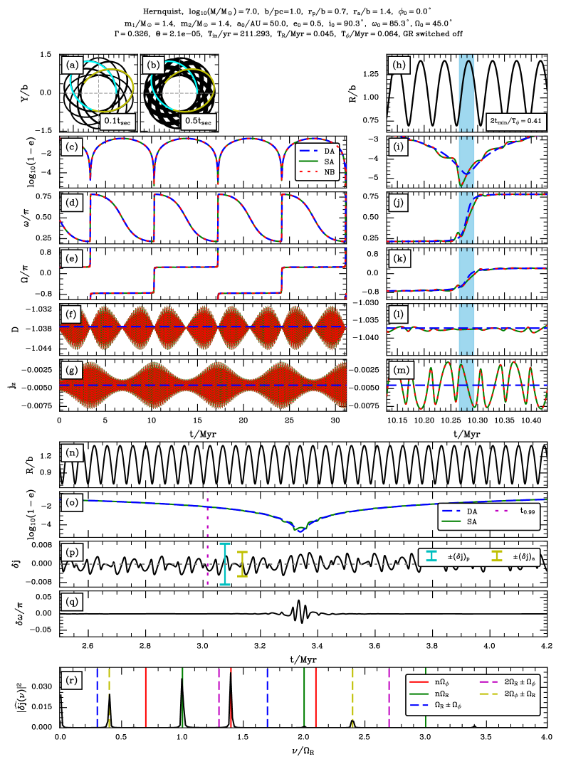
Figure 3.— Example of a binary that undergoes significant short-timescale fluctuations at very high eccentricity (the same one we used in Figure 1). The details of the plot are explained fully in §3.1. Note the initial inclination $i_{0}=90.3^{\circ}$. The DA secular period is $t_{\mathrm{sec}}\approx 6.9$ Myr.

In Figure 3 we give an example of a binary that undergoes significant short-timescale fluctuations at high eccentricity. This figure is very rich in information and exhibits several interesting features that we wish to explore throughout the paper. We will also see several other figures with this or similar structure. It is therefore worth describing the structure of Figure 3 in detail.

At the very top of the figure (top line of text) we provide the values of 6 input parameters ($\Phi,\,\mathcal{M},\,b,\,r_{\mathrm{p}},\,r_{\mathrm{a}},\,\phi_{0}$) that define the perturbing potential as well as the outer orbit’s initial conditions. In this case (which is the same setup as in Figure 1) we are considering a binary in a Hernquist potential $\Phi(r)=-G\mathcal{M}/(b+r)$, with total mass $\mathcal{M}=10^{7}M_{\odot}$ and scale radius $b=1\mathrm{pc}$. Since this potential is spherical, the shape of the outer orbit is determined by two numbers: its pericenter distance $r_{\mathrm{p}}=0.7b$, its apocenter $r_{\mathrm{a}}=1.4b$. Unless otherwise specified, in this paper we always initiate the outer orbit at $t=0$ from $(R,\phi)=(r_{\mathrm{p}},\phi_{0})$ with $\dot{\phi}>0$, where $\phi$ is the outer orbit’s azimuthal angle relative to the $X$ axis (see Paper I).

In the second line of text we list 7 input parameters $(m_{1},\,m_{2},\,a_{0},\,e_{0},\,i_{0},\,\omega_{0},\,\Omega_{0})$ that concern the binary’s inner orbit; the subscript ‘$0$’ denotes initial values. In this example we are considering a NS-NS binary ($m_{1}=m_{2}=1.4M_{\odot}$) with initial semimajor axis $a_{0}=50\mathrm{AU}$. Note also that the initial inclination $i_{0}$ is chosen close to $90^{\circ}$, which is necessary to achieve very large eccentricities starting from $e_{0}\ll 1$ (since this requires $\Theta\ll 1$).

In the third and final line of text at the top of the figure, we list 5 important quantities that follow from the choices of 13 input parameters above: $\Gamma,\Theta$, the inner orbital period $T_{\mathrm{in}}=2\pi\sqrt{\mu/a^{3}}$, the outer orbit’s radial period $T_{R}$, and its azimuthal period $T_{\phi}$. In this instance we have a $\Gamma$ value of $0.326$ and $\Theta=2.1\times 10^{-5}$, which allows $e_{\mathrm{max}}$ to become extremely high. Lastly, we emphasise that we have artificially switched off GR precession in this example. Thus we set $\epsilon_{\mathrm{GR}}=0$ in the equations of motion and in evaluating $D$, which is equivalent to taking the speed of light $c\to\infty$. This choice is also indicated in the third line of text. GR precession will be incorporated in §4, allowing for direct comparison with the results of this section.

Now we move on to the figure proper. In panels (a) and (b) we display the trajectory of the outer orbit through the $(X,Y)$ plane, integrated using GALPY (Bovy, 2015). In both panels we show the trajectory from $t=0$ to $t=T_{R}$ (cyan line), and from $t=T_{R}$ to $t=2T_{R}$ (yellow line). In black we show the entire trajectory traced up to time $t=0.1t_{\mathrm{sec}}$ (panel (a)) and $t=0.5t_{\mathrm{sec}}$ (panel (b)), where $t_{\mathrm{sec}}$ is the period of secular oscillations, computed using equation (33) of Paper II.

In total we integrated the outer orbit $\mathbf{R}_{\mathrm{g}}(t)$ until $t=4.5t_{\mathrm{sec}}$. We then fed the resulting $\Phi_{\mathrm{\alpha\beta}}(\mathbf{R}_{\mathrm{g}}(t))$ time series into the SA quadrupolar equations of motion (A1)-(A4) and integrated them numerically. In panels (c), (d) and (e) we compare the numerical integrations of the SA equations of motion for $e$, $\omega$, $\Omega$ (green curves) against the prediction of DA theory (blue dashed curves). We also show the results of direct orbit integration (red dotted curves), where we evolved the exact two-body equations of motion of the binary in the presence of the smooth time-dependent external field $\Phi(\mathbf{R}_{\mathrm{g}}(t))$ without any tidal approximation, using the N-body code REBOUND (Rein & Liu, 2012). In panel (c) we see that the binary reaches extremely high eccentricity, with the DA result $1-e_{\mathrm{DA}}$ reaching a minimum at $\approx 10^{-4.8}$. In this panel we already see that the maximum eccentricity reached in the SA approximation can be rather different from the DA value, and changes from one eccentricity peak to the next — near the second peak, around $10$ Myr, $1-e_{\mathrm{SA}}$ plunges to $\sim 10^{-5.4}$. On the other hand, the agreement between the SA and direct orbit integration integrations is excellent, which gives us confidence that the numerics is accurate and that the quadrupolar approximation is a good one (see also §§5.2-5.4). Another striking feature of panels (d) and (e) is the step-like jumps in $\omega$ and $\Omega$ that occur near maximum eccentricity in both SA and DA integrations. These are just what we expect from our investigation in Appendix C of Paper III.

In panels (f) and (g) we show the evolution of the quantities $D$ (equation (13)) and $j_{z}$ (equation (5)). In the DA approximation, $D$ and $j_{z}$ are integrals of motion — hence the blue dashed DA result is simply a straight horizontal line. We see that the SA result oscillates around the constant DA value in both cases, with an envelope that has period $t_{\mathrm{sec}}$ for $j_{z}$ and $t_{\mathrm{sec}}/2$ for $D$. In panel (f) there is in fact a small offset between $D_{\mathrm{DA}}$ and the mean value of $D_{\mathrm{SA}}$, which is due to an initial phase offset of the outer orbit (Luo et al. 2016; Grishin et al. 2018). We also notice a characteristic behavior which is that fluctuations in $D$ are minimised around the eccentricity peak, while fluctuations in $j_{z}$ are maximised there.

In the right hand column, in panels (i)-(m) we simply reproduce panels (c)-(g), except we zoom in on the sharp eccentricity peak at around $10.28\,\mathrm{Myr}$. At the top of this column we have panel (h), which shows the outer orbital radius $R(t)$ during this high-eccentricity episode. In addition, in each panel (h)-(m) we shade in light blue the region

$$t(j_{\mathrm{min}})-t_{\mathrm{min}}<t<t(j_{\mathrm{min}})+t_{\mathrm{min}}.$$ (14)

Here $t(j_{\mathrm{min}})$ is the time corresponding to the minimum of $j_{\mathrm{DA}}$ (i.e. peak DA eccentricity), namely when $j_{\mathrm{DA}}=j_{\mathrm{min}}$, and $t_{\mathrm{min}}$ is the time taken for $j_{\mathrm{DA}}$ to change from $j_{\mathrm{min}}$ to $\sqrt{2}j_{\mathrm{min}}$ — see §4.2 of Paper III. In panel (h) we also indicate the value of the ratio $2t_{\mathrm{min}}/T_{\phi}$, which will turn out to be very important when we switch on GR in §4. In this particular case we see that $2t_{\mathrm{min}}/T_{\phi}=0.41$, so that most of the interesting (very highest eccentricity) behavior happens on a timescale shorter than an outer azimuthal period.

From panels (i)-(m) we see that the SA integration (green lines) agrees very well with the direct orbit integration (red dashed lines) even at very high eccentricities, giving us confidence that the SA approximation is a good one here. However, the SA prediction differs markedly from the DA prediction at very high eccentricity. In particular, from panel (i) we see that $1-e_{\mathrm{DA}}$ becomes $\approx 10^{-4.6}$ at its minimum, while $1-e_{\mathrm{SA}}$ reaches a significantly smaller value still, $\approx 10^{-5.4}$. Panels (j) and (k) reveal that the large jumps in $\omega$ and $\Omega$ both happen on a timescale $\sim 2t_{\mathrm{min}}$. In panels (l) and (m) we show how the integrals of motion $j_{z}$ and $D$ fluctuate around the maximum eccentricity.

In panels (n)-(q) we again show the time series of $R$ and $1-e$ around the second eccentricity peak (although over a wider timespan), as well as the differences

$$\delta j(t)\equiv j_{\mathrm{SA}}(t)-j_{\mathrm{DA}}(t),\,\,\,\,\,\,\,\,\delta\omega(t)\equiv\omega_{\mathrm{SA}}(t)-\omega_{\mathrm{DA}}(t),$$ (15)

between the results of SA and DA integration. The vertical dotted magenta line in panels (o) and (p) corresponds to $t=t_{0.99}$, which is the time when $e_{\mathrm{DA}}$ first reaches $0.99$. From panel (p) we see that $\delta j$ fluctuates in a complex but near-periodic manner, with period $\sim 5T_{R}$. The fluctuations themselves are not perfectly centered around zero; before the eccentricity peak, the mean value of $\delta j$ is slightly negative, whereas afterwards it is slightly positive. The blue and cyan bars in panel (p) correspond to simple approximations to the amplitude of $\delta j$ at peak eccentricity — see §3.3. Meanwhile, from panel (q) we see that the fluctuation $\delta\omega$ is negligible until the very highest eccentricities are reached, where there is a sharp pulse before it decays to zero again. This pulse is approximately antisymmetric in time around $t=t(j_{\mathrm{min}})$. The pulse episode lasts for $\sim 2T_{R}$.

Finally, in panel (r) we show the power spectrum of $\delta j$ fluctuations, which is the square of the Fourier transform $\widehat{\delta j}(\nu)\equiv\int\mathrm{d}t\exp(i\nu t)\delta j(t)$. We calculated this Fourier transform numerically using the $\delta j(t)$ data from panel (p). We see that the signal is concentrated at frequencies $\nu=n_{1}\Omega_{R}+n_{2}\Omega_{\phi}$ for certain pairs of integers $n_{1}$, $n_{2}$, where $\Omega_{i}\equiv 2\pi/T_{i}$ is the outer orbital frequency. We discuss these power spectra briefly in §3.3 and §4.2.3.

3.1.2 Further examples

In Appendix C we give two more numerical examples, which display behavior mostly similar to that just described. They differ from Figure 3 in that in the first one (Figure 18), the initial inclination is changed to $i_{0}=93.3^{\circ}$, and in the second one (Figure 19), the Hernquist potential is replaced with a Plummer potential. They will also give rise to very different behavior when they are run with GR precession switched on, as we will see in §4. We will refer to these Figures throughout the rest of the paper.

3.2. Analysis of fluctuating behavior

We now wish to explain more quantitatively the behavior that we observed in §3.1. Precisely, we aim to understand the characteristic behaviors of $\delta j$ and $\delta\omega$ around the eccentricity peak and to understand the envelopes of $D$ and $j_{z}$ fluctuations over secular timescales. We will address the separate problem of determining the amplitude of fluctuations $\delta j$ around the peak eccentricity in §3.3. All this is necessary for understanding the nature of RPSD in Section 4.2.

3.2.1 Notation

To achieve these aims we must first introduce a clean, precise notation to describe fluctuations. Let us define the vector $\mathbf{w}\equiv[\omega,J,\Omega,J_{z}]$. Then the ‘SA solution’

$$\mathbf{w}_{\mathrm{SA}}(t)\equiv[\omega_{\mathrm{SA}}(t),J_{\mathrm{SA}}(t),\Omega_{\mathrm{SA}}(t),J_{z,\mathrm{SA}}(t)],$$ (16)

is found by self-consistently integrating the SA equations (A1)-(A4), which are the Hamilton equations resulting from $H_{\mathrm{SA}}(\omega_{\mathrm{SA}},J_{\mathrm{SA}},\Omega_{\mathrm{SA}},J_{z,\mathrm{SA}},t)\equiv H_{\mathrm{SA}}(\mathbf{w}_{\mathrm{SA}},t)$. Meanwhile the ‘DA solution’

$$\mathbf{w}_{\mathrm{DA}}(t)\equiv[\omega_{\mathrm{DA}}(t),J_{\mathrm{DA}}(t),\Omega_{\mathrm{DA}}(t),J_{z,\mathrm{DA}}],$$ (17)

is found by self-consistently integrating the DA equations of motion, which are the Hamilton equations for $H_{\mathrm{DA}}(\omega_{\mathrm{DA}},J_{\mathrm{DA}},J_{z,\mathrm{DA}})\equiv H_{\mathrm{DA}}(\mathbf{w}_{\mathrm{DA}})$. Consistent with equation (15) we formally define:

$$\delta\mathbf{w}(t)\equiv\mathbf{w}_{\mathrm{SA}}(t)-\mathbf{w}_{\mathrm{DA}}(t).$$ (18)

Next, we will also find it useful to define a ‘fluctuating Hamiltonian’:

$$\Delta H(\mathbf{w},t)\equiv H_{\mathrm{SA}}(\mathbf{w},t)-H_{\mathrm{DA}}(\mathbf{w}),$$ (19)

which is written out explicitly in Appendix D. Using $\Delta H$, we can define four new quantities

$$\Delta\mathbf{w}(\mathbf{w},t)\equiv[\Delta\omega(\mathbf{w},t),\Delta J(\mathbf{w},t),\Delta\Omega(\mathbf{w},t),\Delta J_{z}(\mathbf{w},t)],$$ (20)

as the solution to the equations of motion

$$\frac{\mathrm{d}\Delta\mathbf{w}(\mathbf{w},t)}{\mathrm{d}t} \equiv\left[\frac{\partial}{\partial J},-\frac{\partial}{\partial\omega},\frac{\partial}{\partial J_{z}},-\frac{\partial}{\partial\Omega}\right]\Delta H(\mathbf{w},t).$$ (21)

As an example, the partial derivative $\partial\Delta H/\partial\omega$ is given explicitly for spherical potentials in equation (D5).

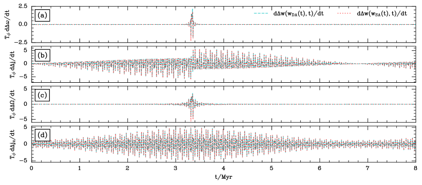
Figure 4.— Time series of $\mathrm{d}\Delta\mathbf{w}/\mathrm{d}t$ following the definition (21), for the first $8$ Myr of evolution from Figure 3 (the first peak in DA eccentricity occurs at $t\approx 3.34$Myr; the subsequent eccentricity minimum is at $t\approx 6.8$Myr). Cyan dashed lines and red dotted lines show $\mathrm{d}\Delta\mathbf{w}(\mathbf{w}_{\mathrm{SA}},t)/\mathrm{d}t$ and $\mathrm{d}\Delta\mathbf{w}(\mathbf{w}_{\mathrm{SA}},t)\mathrm{d}t$ respectively.

Note that equation (21) is defined for arbitrary arguments $\mathbf{w}$. In Figure 4 we plot the time series of $\mathrm{d}\Delta\mathbf{w}(\mathbf{w},t)/\mathrm{d}t$ for $\mathbf{w}=\mathbf{w}_{\mathrm{DA}}$ and $\mathbf{w}=\mathbf{w}_{\mathrm{SA}}$ using the data from the first $8$ Myr of evolution from Figure 3. Repeating the same exercise for other examples gives plots that look qualitatively the same as Figure 4.

Now we must bear in mind that in general,

$$\delta\mathbf{w}(t)\neq\Delta\mathbf{w}(\mathbf{w}_{\mathrm{SA}}(t),t)\neq\Delta\mathbf{w}(\mathbf{w}_{\mathrm{DA}}(t),t).$$ (22)

Nevertheless, for our purposes it is normally sufficient to approximate

$$\delta\mathbf{w}(t)\approx\Delta\mathbf{w}(\mathbf{w}_{\mathrm{SA}}(t),t)\approx\Delta\mathbf{w}(\mathbf{w}_{\mathrm{DA}}(t),t).$$ (23)

In Appendix E we explain why this is the case, and justify it with a numerical example.

3.2.2 Scaling of fluctuations at high eccentricity in spherical cluster potentials

Having established the approximation (23), we can use the equations of motion (21) to gain a better understanding of the behavior of fluctuating quantities $\delta\mathbf{w}$ in Figures 3 and 19. To do this we take derivatives of $\Delta H$ as given in (D4) (which is valid for spherical potentials only) and then take the high eccentricity limit $L^{2}\gg J^{2}\gtrsim J_{z}^{2}$. As a result we find the following scalings:

$$\frac{\mathrm{d}}{\mathrm{d}t}\delta j\propto J^{0},\,\,\,\,\,\,\,\,\frac{\mathrm{d}}{\mathrm{d}t}\delta j_{z}\propto J^{0},$$

$$\frac{\mathrm{d}}{\mathrm{d}t}\delta\omega\propto J^{-1},\,\,\,\,\,\,\,\,\frac{\mathrm{d}}{\mathrm{d}t}\delta\Omega\propto J^{-1}.$$ (24)

Thus, we expect the fluctuations $\delta j$, $\delta j_{z}$ to be independent of $j$ as $e\to 1$, i.e. as $j^{2},\,j_{z}^{2}\to 0$. In other words, as the binary approaches maximum eccentricity we do not expect any sharp peak in $\delta j(t)$ or $\delta j_{z}(t)$, but we do expect a spike in $\delta\omega(t)$ and $\delta\Omega(t)$. Such behavior is precisely what we found in panels (m), (p) and (q) of Figures 3 and 19, and is also exhibited clearly in Figure 21.

3.2.3 Envelope of fluctuations in $D$ and $j_{z}$

In the numerical examples above, fluctuations in $j_{z,\mathrm{SA}}$ consisted of rapid oscillations on the timescales $\sim T_{\phi},T_{R}$ (reflective of the torque fluctuating on the outer orbital timescale), modulated by an envelope with period $t_{\mathrm{sec}}$. Similarly, $D_{\mathrm{SA}}$ oscillated on the timescale $\sim T_{\phi}$, modulated by an envelope with period $t_{\mathrm{sec}}/2$. We now explain each of these envelope behaviors in turn.

First, we consider the envelope of $j_{z,\mathrm{SA}}$ fluctuations. It is clear from the numerical examples that the amplitude of this envelope is largest around the eccentricity peak (minimum $j$), and smallest around the eccentricity minimum (maximum $j$). This is easily explained by evaluating the torque formula $\mathrm{d}j_{z,\mathrm{SA}}/\mathrm{d}t$ using equations (21) and (D6), and examining the scaling with $j$ (which is well illustrated by the example in Figure 4d). The envelope of $j_{z}$ fluctuations simply reflects the amplitude of the fluctuating torque.

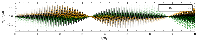
Figure 5.— Time series of $\mathrm{d}D/\mathrm{d}t$ (black solid line) for the first $8$ Myr of evolution from Figure 3, following equation (25). The green and orange dotted lines show contributions from $\dot{D}_{1}$ (equation (26)) and $\dot{D}_{2}$ (equation (27)) respectively. The amplitude of both terms is smallest at the extrema of $e_{\mathrm{DA}}$.

Second, we address the fluctuations in $D_{\mathrm{SA}}$. In this case the amplitude of the envelope exhibits minima at times corresponding to both $j_{\mathrm{DA}}=j_{\mathrm{max}}$ and $j_{\mathrm{DA}}=j_{\mathrm{min}}$, and maxima in-between. To see why, we differentiate (13) with $\epsilon_{\mathrm{GR}}$ set to zero:

$$\frac{\mathrm{d}D}{\mathrm{d}t}=\dot{D}_{1}+\dot{D}_{2}$$ (25)

where

$$\dot{D}_{1} = \frac{2\,D(\epsilon_{\mathrm{GR}}=0)}{e}\frac{\mathrm{d}e}{\mathrm{d}t}=-\frac{2j\,D(\epsilon_{\mathrm{GR}}=0)}{1-j^{2}}\frac{\mathrm{d}j}{\mathrm{d}t},$$ (26)

$$\dot{D}_{2} = \frac{10\Gamma e^{2}}{1-5\Gamma}\frac{\mathrm{d}}{\mathrm{d}t}\left(\sin^{2}i\sin^{2}\omega\right).$$ (27)

In Figure 5 we plot $\mathrm{d}D/\mathrm{d}t$ following equation (25), again over the first $8$ Myr of evolution from Figure 3. With green and orange dotted lines we overplot the contributions coming from $\dot{D}_{1}$ and $\dot{D}_{2}$ respectively. Like with $j_{z,\mathrm{SA}}$, the envelope of fluctuations in $D_{\mathrm{SA}}$ reflects the envelope of $\mathrm{d}D/\mathrm{d}t$. In particular, the amplitudes of both $\dot{D}_{1}$ and $\dot{D}_{2}$ are minimized at the eccentricity extrema, and maximized in-between. A much more detailed discussion of $\mathrm{d}D/\mathrm{d}t$ at high eccentricity is postponed to §4.2.1.

3.3. Characteristic amplitude of $\delta j$ fluctuations

Perhaps the most important consequence of short-timescale fluctuations is that they enhance the value of $e_{\mathrm{max}}$ when $e$ gets very large, which can lead to e.g. more rapid compact object binary mergers (Grishin et al., 2018). With this in mind, we wish to estimate $(\delta j)_{\mathrm{max}}$, which we define to be the absolute value of the maximum fluctuation $\delta j$ in the vicinity of maximum eccentricity. Unfortunately, a given binary does not have a single value of $(\delta j)_{\mathrm{max}}$, because the precise details of the fluctuating behavior differ from one secular eccentricity peak to the next. (We already saw something closely related to this in Figure 1b, where binaries which approached the same secular eccentricity peak with different outer orbital phases ended up exhibiting very different behavior around $e_{\mathrm{max}}$). In Appendix F, we show how to estimate the characteristic size of such fluctuations and then demonstrate numerically that our estimate is a reasonable one, culminating in equations (F3) and (F5).

The problem with equations (F3) and (F5) as they stand is that we do not know precisely which quarter-period in $\phi$ will provide the dominant fluctuation, because this would require knowledge of $R(t)$ and $\phi(t)$. Thus, we cannot evaluate (F5) directly for an arbitrary outer orbit — and even if we could, we would not expect the resulting $(\delta j)_{\mathrm{max}}$ to be exactly correct because of the non-stationarity of $\omega,j,\Omega$.

However, we can make a very rough estimate of the importance of these fluctuations if we note that $F$ is normally of the same order of magnitude as the azimuthal frequency of the outer orbit, $2\pi/T_{\phi}$. Then using $\cos i_{\mathrm{min}}\sim 1$ and the weak GR result $j_{\mathrm{min}}^{2}\sim\Theta\sim\cos^{2}i_{0}$, we get

$$\frac{(\delta j)_{\mathrm{max}}}{j_{\mathrm{min}}}\sim\frac{1}{|\cos i_{0}|}\frac{T_{\mathrm{in}}}{T_{\phi}}.$$ (28)

This equation is useful for estimating whether the effect of short-timescale fluctuations can drastically change $j$ at very high eccentricity. In particular, it tells us that SA effects are crucial for binaries with initial inclinations in the range

$$|\cos i_{0}|\lesssim\frac{T_{\mathrm{in}}}{T_{\phi}}.$$ (29)

We can also relate the estimate (28) to the ratio $t_{\mathrm{min}}/T_{\phi}$, which will be a very important parameter in our discussion of RPSD (see §4). We know from Paper II that $t_{\mathrm{sec}}\sim T_{\phi}^{2}/T_{\mathrm{in}}$. Then the time spent near highest eccentricity (equation (3)) is on the order of $t_{\mathrm{min}}\sim j_{\mathrm{min}}t_{\mathrm{sec}}\sim j_{\mathrm{min}}T_{\phi}^{2}/T_{\mathrm{in}}$. Using this to eliminate $T_{\mathrm{in}}$ from the right hand side of (28) gives

$$\frac{(\delta j)_{\mathrm{max}}}{j_{\mathrm{min}}}\sim\frac{T_{\phi}}{t_{\mathrm{min}}}.$$ (30)

Thus short-timescale fluctuations are important in precisely those regions of parameter space where $t_{\mathrm{min}}$ is comparable to or smaller than $T_{\phi}$.

4. The effect of GR precession

In the previous section we gained insight into how short-timescale fluctuations in the tidal torque affect high eccentricity behavior, but if our results are to be relevant for studying dynamical compact object merger channels, then it is vital that we also account for 1pN GR precession. As we will see in this section, including GR precession can change the picture significantly. To begin with, in §4.1 we rerun the numerical calculations from §3.1 except this time with GR precession switched on, and simply describe the altered phenomenology. In §4.1.5 we compare the GR and non-GR calculations in the special case of the LK problem. The main new result that arises in each of these subsections is RPSD, which stems from non-conservation of the approximate integral of motion $D$ in the SA approximation. In §4.2 we offer a physical explanation for this new phenomenon, explain the criteria for its existence, and attempt a rough statistical analysis.

4.1. Numerical examples with GR precession

4.1.1 Fiducial Hernquist example

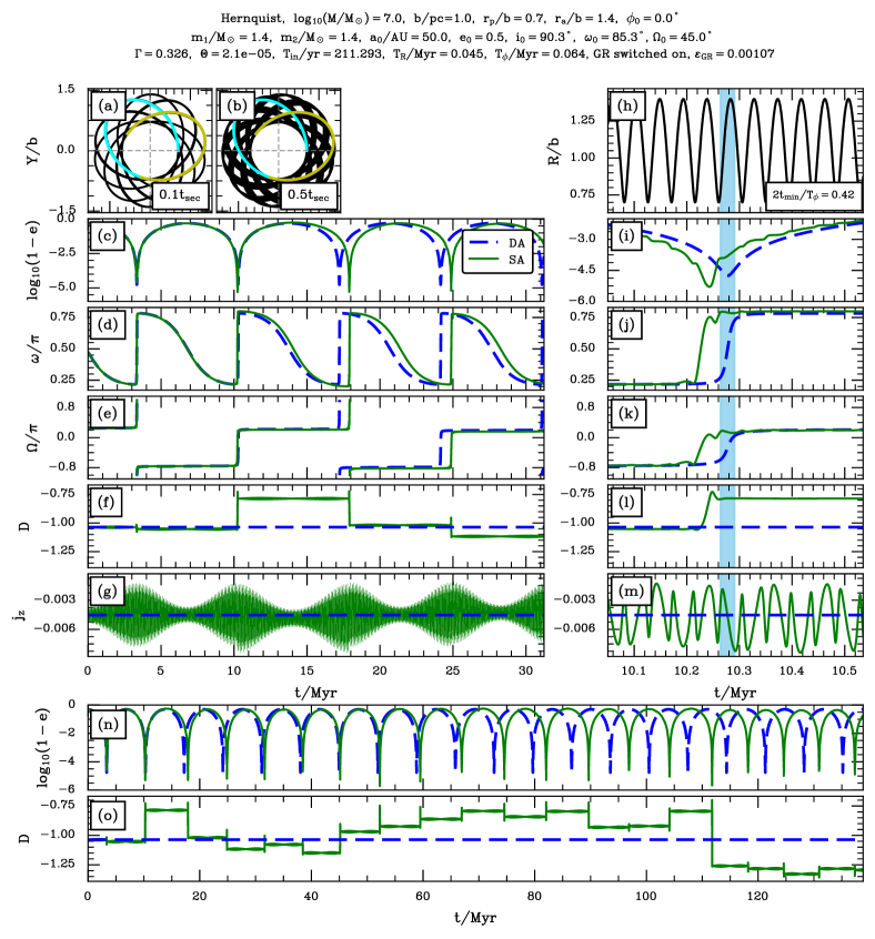
Figure 6.— As in Figure 3, except we switch on GR precession. This causes the time-averaged value of $D_{\mathrm{SA}}$ to diffuse away from $D_{\mathrm{DA}}$, with discrete jumps occurring during episodes of extremely high eccentricity. We call this relativistic phase space diffusion (‘RPSD’).

In Figure 6 we rerun the calculation from Figure 3, except we switch on the GR precession term (with strength $\epsilon_{\mathrm{GR}}=0.00107$) in the SA and DA equations of motion. We now discuss Figure 6 in some detail.

The structure of panels (a)-(m) is identical to those of Figure 3, except that we have dispensed with direct orbit integration since it is prohibitively computationally expensive (to capture accurately the fast GR precession during eccentricity peaks tends to require an extremely tiny timestep). Comparing panels (a)-(m) with those of Figure 3 we immediately notice several qualitative differences. Whereas in Figure 3 the DA and SA predictions for $\log_{10}(1-e)$ agreed almost perfectly except at extremely high eccentricity, now in Figure 6 (with GR precession switched on) they disagree manifestly after the second eccentricity maximum. Moreover, while the period of secular oscillations is fixed in the DA case, the SA secular period changes from one eccentricity peak to the next. By the time of the third eccentricity peak the DA and SA curves in panels (c)-(e) are completely out of sync, as we intimated would happen back in §1.1, when we were discussing Figure 2.

Crucially, from panel (f) we see that $D_{\mathrm{SA}}$ no longer fluctuates around $D_{\mathrm{DA}}$ indefinitely like it did in Figure 3f, but rather exhibits discrete jumps during very high eccentricity episodes. In panel (l) we zoom in on the $D_{\mathrm{SA}}$ behavior around the second eccentricity peak. We see that $D_{\mathrm{SA}}$ jumps from $\approx-1.05$ to $\approx-0.8$ and that this jump happens on the timescale $\sim 2t_{\mathrm{min}}$ (the width of the blue shaded band). This jump in the approximate integral of motion $D$ means that the binary has jumped to a new constant-Hamiltonian contour in the DA $(\omega,e)$ phase space (Papers II-III), as we confirm in Figure 7. Since this behavior depends crucially on the presence of finite GR precession we choose to call it ‘relativistic phase space diffusion’ (RPSD). Furthermore, each phase space contour has its own secular period, i.e. the secular period $t_{\mathrm{sec}}$ depends on $D$ (see §2.6 of Paper II, and especially Figure 3 of that paper). Hence it is unsurprising that a jump in $D_{\mathrm{SA}}$ leads to a modified SA secular period compared to the fixed DA period.

Meanwhile, we observe in panel (g) that the envelope of $j_{z,\mathrm{SA}}$ fluctuations does undergo abrupt, although very modest, changes that coincide with the second and third eccentricity peaks. Thus, the adiabatic invariance of $j_{z,\mathrm{SA}}$ is also slightly broken, but its time average is much better preserved than is the time average of $D_{\mathrm{SA}}$.

To investigate the RPSD behavior further, we next ran the integration for a much longer time, $20t_{\mathrm{sec}}$. In panels (n) and (o) of Figure 6 we plot $1-e$ and $D$ respectively as functions of time over this entire duration. The same picture holds in that $D_{\mathrm{SA}}$ is roughly static between eccentricity peaks, but often makes a discernible jump during a peak. These jumps seem to have no preferred sign.

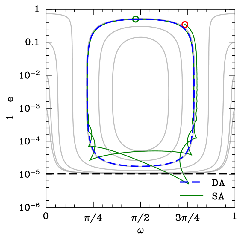
Figure 7.— Illustration of RPSD in phase space. We plot the trajectory of the binary from Figure 6 through the $(\omega,e)$ phase space, over the first $\sim 2t_{\mathrm{sec}}$. We show the DA trajectory in blue and the SA trajectory in green. The grey lines are contours of constant DA Hamiltonian (equations (9) and (10)), and the black dashed line gives the maximum achievable DA eccentricity $e_{\mathrm{lim}}\equiv\sqrt{1-\Theta}$, all calculated at $t=0$. The binary’s initial phase space location is shown with a green circle, and this of course coincides with the blue dashed contour on which the DA solution lives indefinitely. The binary’s final SA location is shown with a red circle. We see that the SA trajectory jumps to a new ‘parent’ DA contour (i.e. off the blue dashed DA contour) during the second high eccentricity episode.

4.1.2 Changing the initial inclination to $i_{0}=93.3^{\circ}$

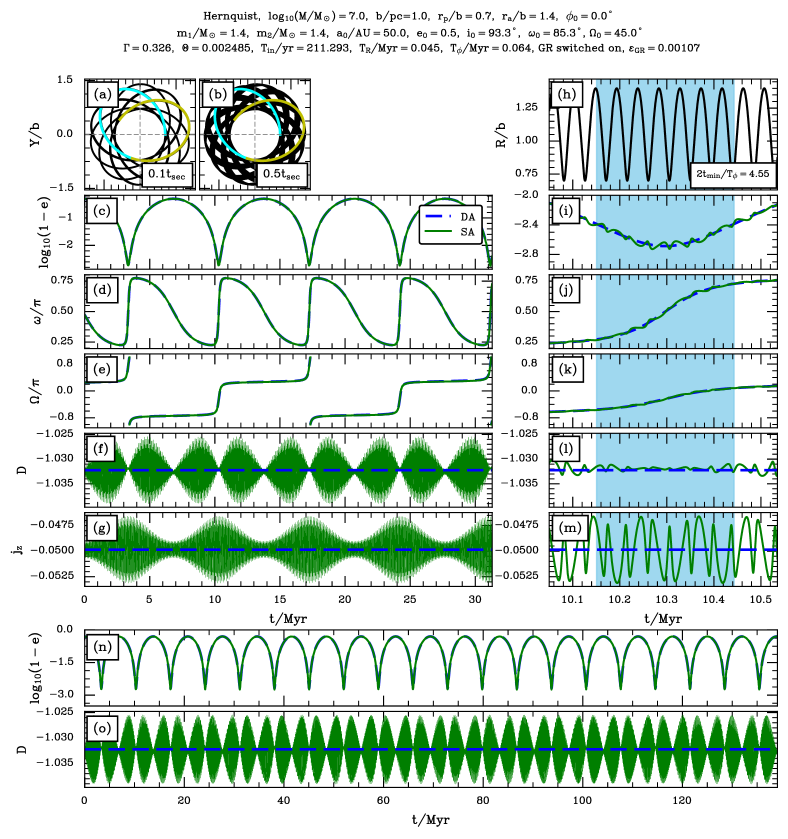
Figure 8.— As in Figure 6 except we take $i_{0}=93.3^{\circ}$ — in other words, the same as Figure 18 except we switch on GR precession. There is no RPSD in this case.

RPSD does not occur in Figure 8, in which we keep the initial conditions exactly the same as Figure 6 except that we change $i_{0}$ from $90.3^{\circ}$ to $93.3^{\circ}$. (In other words, we rerun the same calculation as in Figure 18 except with GR switched on). Note that this case has $2t_{\mathrm{min}}/T_{\phi}=4.55$, as opposed to Figure 6 which had $2t_{\mathrm{min}}/T_{\phi}=0.42$.

4.1.3 An example in the Plummer potential

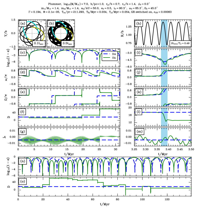
Figure 9.— Fiducial Plummer example including GR precession. As in Figure 6 except we use the Plummer potential — in other words, the same as Figure 19 except we switch on GR precession. In this case, after a few secular periods the DA prediction does not even qualitatively describe the SA dynamics.

In Figure 9 we give another example of RPSD, this time in the Plummer potential. This example is identical to that in Figure 19 except that we switched on GR precession, and zoomed in on the first eccentricity peak in the right column rather than the second. Panel (l) shows that this first eccentricity peak coincides with a large jump in $D$. As a result, the subsequent SA evolution is entirely different from the original DA prediction.

4.1.4 Dependence on phase angles

Analogous to the discussion in §C.3, we have also run several more numerical calculations identical to those shown in this section but varying the outer orbit’s initial radial phase angle and the initial value of $\phi-\Omega$. As expected from Figure 2, we find that RPSD is highly phase-dependent, meaning that SA simulations run with slightly different initial conditions can have dramatically different outcomes. This suggests we should attempt a statistical analysis — see §4.2.3.

4.1.5 An example in the Lidov-Kozai limit

It is important to note that RPSD is not exclusive to the non-Keplerian potentials that we have investigated so far, but is present in the Lidov-Kozai problem as well, at the test-particle quadrupole level (though to our knowledge, nobody has mentioned it explicitly).

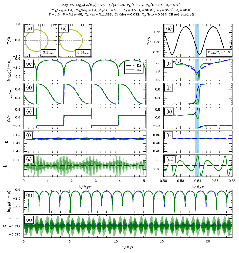
Figure 10.— As in Figure 3, except we use the Kepler potential (so we are studying the classic test-particle quadrupole Lidov-Kozai mechanism). GR precession is switched off here.

To demonstrate this, in Figure 10 we show a calculation with exactly the same initial condition as in Figure 3, except that we change the potential to the Keplerian one, $\Phi=-G\mathcal{M}/{R}$. In other words, we are now investigating the classic test particle quadrupole Lidov-Kozai problem, relevant to e.g. a NS-NS binary orbiting a SMBH (e.g. Antonini & Perets 2012; Hamers 2018; Bub & Petrovich 2020), except that we have GR precession switched off. In panels (a) and (b) we simply see the outer orbital ellipse, which has semimajor axis $a_{\mathrm{g}}=(r_{\mathrm{a}}+r_{\mathrm{p}})/2=1.05b$ and eccentricity $e_{\mathrm{g}}=(r_{\mathrm{a}}-r_{\mathrm{p}})/(r_{\mathrm{a}}+r_{\mathrm{p}})=0.33$. Panels (c)-(m) exhibit behavior which is qualitatively similar to that in Figure 3. Since $2t_{\mathrm{min}}/T_{\phi}=0.15$, the highest eccentricity episode lasts for significantly less than one outer orbital period. Despite this, the SA result tracks the secular (DA) result indefinitely. (We have also checked that the SA result shown here is indistinguishable from that found by direct orbit integration).

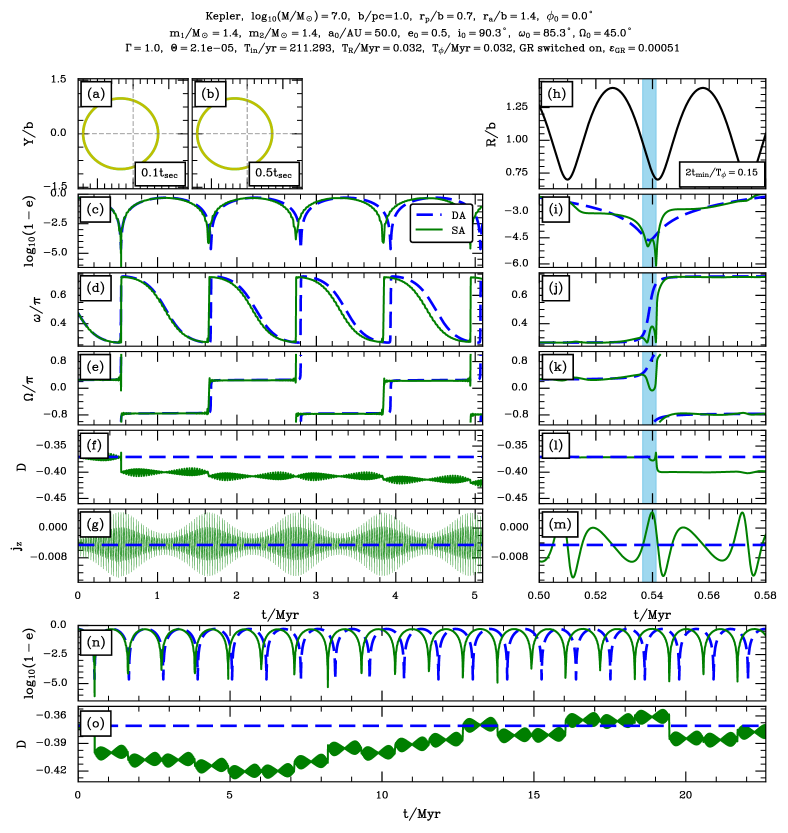
Figure 11.— As in Figure 10 except with GR precession switched on. This Figure shows that RPSD is present even in the test-particle quadrupole LK problem as long as GR is included.

Next, in Figure 11 we perform the same calculation as in Figure 10, but now with GR precession switched on. This causes significant and repeated diffusion of $D_{\mathrm{SA}}$ around the secular eccentricity peaks, meaning the binary ultimately follows a completely different SA trajectory compared to the one we would have predicted had we only used DA theory. This confirms that RPSD is present as a phenomenon in LK theory at the test-particle quadrupole level as long as 1pN GR precession is included.

4.2. Physical interpretation of RPSD and quantitative analysis

The aim of this section is to provide some physical understanding of RPSD and to attempt a rough quantitative analysis of this phenomenon.

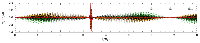
Figure 12.— Time series of $\mathrm{d}D/\mathrm{d}t$ (equation (31)) for the first $8$ Myr of evolution from Figure 6; in other words, this is the counterpart of Figure 5 with GR included. The green and orange dotted lines again show the contributions from $\dot{D}_{1}$ and $\dot{D}_{2}$ (equations (26)-(27)), whereas the red dashed line shows (32); the black solid line is the total $\mathrm{d}D/\mathrm{d}t$.

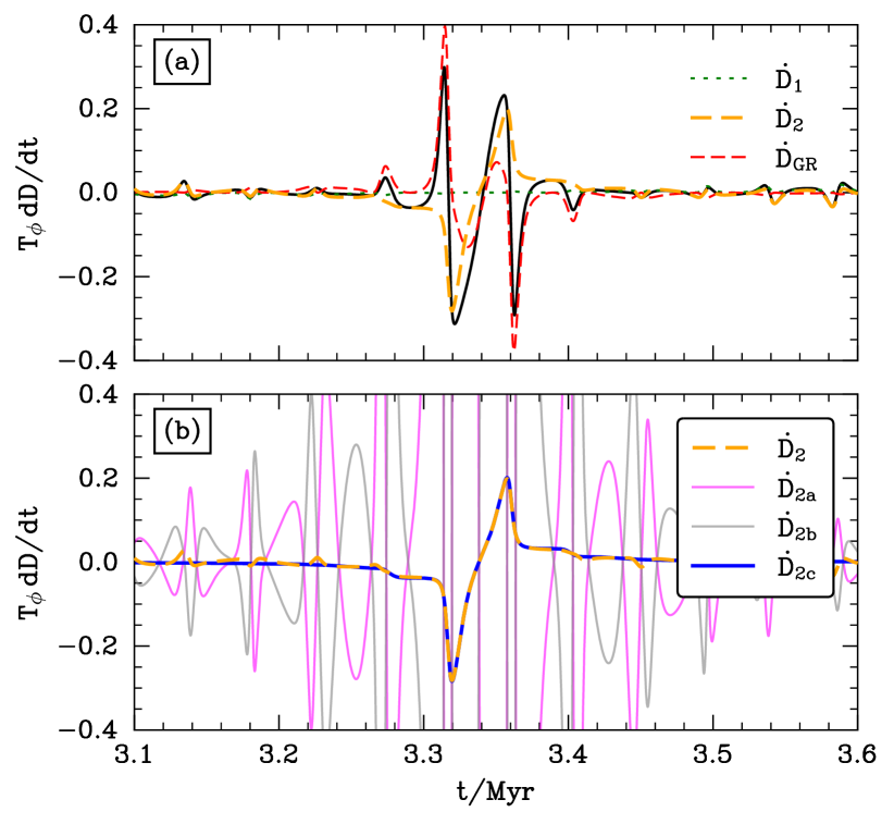
Figure 13.— Panel (a) is the same as in Figure 12, but zoomed in around the first eccentricity peak. In panel (b) we ignore the red, green and black lines from panel (a), leaving only the contribution from the term $\dot{D}_{2}$ (orange), which we decompose into its constituent parts (34)-(36). The terms $\dot{D}_{\mathrm{2a}}$ and $\dot{D}_{\mathrm{2b}}$ have large amplitudes but cancel eachother almost perfectly at high eccentricity.

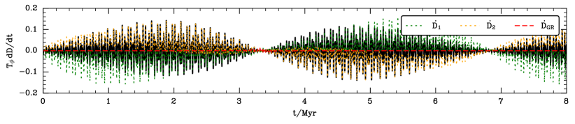
Figure 14.— As in Figure 12, but using data from Figure 8, which does not exhibit RPSD.

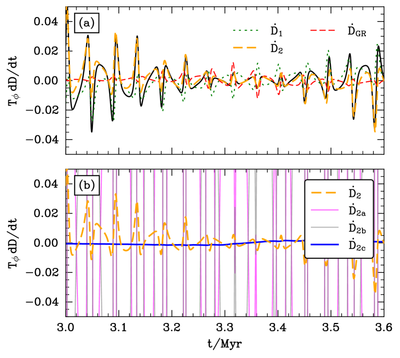
Figure 15.— Panel (a) is as in Figure 14, but zoomed in around the first eccentricity peak. Panel (b) shows $\dot{D}_{2}$ (orange), and its constituent parts (34)-(36).

4.2.1 Mechanism behind RPSD

To understand why RPSD occurs, we take note of two pieces of empirical evidence from the above examples (which we confirmed in several additional numerical experiments not shown here):

• When GR precession is switched off, there is no RPSD.

• RPSD can occur when $2t_{\mathrm{min}}/T_{\phi}\lesssim 1$ but we do not observe it to occur when $2t_{\mathrm{min}}/T_{\phi}\gg 1$.

Taking these strands of evidence together will allow us to identify the physical mechanism behind RPSD, as we now explain.

Whether we consider SA or DA dynamics, at eccentricities far from unity, significant changes in the orbital elements occur only on secular timescales, i.e. timescales much longer than $T_{\phi}$. Of course, $D$ (equation (13)) is a function of these orbital elements. Thus at eccentricities far from unity, $D_{\mathrm{SA}}(t)$ invariably exhibits relatively small and rapid (timescale $\sim T_{\phi}$) oscillations around the constant value $D_{\mathrm{DA}}$. However, at the highest eccentricities $e\to 1$, significant changes in orbital elements can occur on timescales much shorter than $t_{\mathrm{sec}}$. This is true even in DA theory: for instance, in Appendix C of Paper III (which concerned high-$e$ behavior in the limit of weak, but nonzero, GR precession) we saw several numerical examples of binaries whose $\omega_{\mathrm{DA}}$ value is turned through $\sim 90^{\circ}$ or more on the timescale $2t_{\mathrm{min}}$. Now, when $2t_{\mathrm{min}}/T_{\phi}\gg 1$ this evolution is still slow from the point of view of the outer orbit. But in the regime $2t_{\mathrm{min}}/T_{\phi}\lesssim 1$, the DA theory essentially predicts its own demise, since it tells us that $\mathcal{O}(1)$ relative changes in the orbital elements occur on the timescale of the outer orbit, contrary to the fundamental assumption of the DA approximation, namely outer orbit-averaging (Paper I). In that case, it is possible that the fluctuations of SA theory may no longer be considered small, and would no longer oscillate rapidly around the DA orbital elements while those DA elements change significantly.

As an example, consider e.g. Figure 6j, for which $2t_{\mathrm{min}}/T_{\phi}=0.42$. In this case $\omega_{\mathrm{DA}}$ undergoes a large ‘swing’ on the timescale $\sim 2t_{\mathrm{min}}$ near peak DA eccentricity. This time range is so short that $\omega_{\mathrm{SA}}$ does not have a chance to fluctuate around $\omega_{\mathrm{DA}}$ during it. By contrast, consider Figure 8j, for which $2t_{\mathrm{min}}/T_{\phi}=4.55$. In this instance $\omega_{\mathrm{DA}}$ undergoes a swing of very similar magnitude but on a much longer timescale, allowing $\omega_{\mathrm{SA}}$ to perform multiple small fluctuations around $\omega_{\mathrm{DA}}$ while the ‘swing’ is in progress (i.e. within the blue range).

Now let us incorporate GR precession into the discussion. We know (see Figures 3, 10 and 19) that when GR is switched off, the aforementioned short timescale fluctuations do not affect $D_{\mathrm{SA}}$ very dramatically — instead, $D_{\mathrm{SA}}$ just oscillates around the constant value $D_{\mathrm{DA}}$ indefinitely. Indeed, in the absence of GR, $\mathrm{d}D_{\mathrm{SA}}/\mathrm{d}t$ is minimized at very high eccentricity, as we already showed for a particular example in Figure 5. When we do include GR precession, $\mathrm{d}D_{\mathrm{SA}}/\mathrm{d}t$ gets an additional contribution arising from the last term in equation (13): rather than (25) we now have

$$\frac{\mathrm{d}D}{\mathrm{d}t}=\dot{D}_{\mathrm{1}}+\dot{D}_{\mathrm{2}}+\dot{D}_{\mathrm{GR}},$$ (31)

with $\dot{D}_{1}$, $\dot{D}_{2}$ still given by (26)-(27), and

$$\dot{D}_{\mathrm{GR}}\equiv\frac{\epsilon_{\mathrm{GR}}}{3(1-5\Gamma)}\frac{1}{j^{2}}\frac{\mathrm{d}j}{\mathrm{d}t}.$$ (32)

However, the extra term (32) cannot be directly responsible for RPSD, because when integrated across an eccentricity peak it gives zero. (Equivalently, the third term in (13) is unchanged by passing through an eccentricity peak, since it only depends on the value of $j$). Nevertheless, when coupled with the lack of timescale separation $2t_{\mathrm{min}}/T_{\phi}\lesssim 1$, GR is responsible for RPSD, as we will now demonstrate.

In Figure 12a we plot $\mathrm{d}D/\mathrm{d}t$ (black line) using data from the first $8$ Myr of evolution from Figure 6 (c.f. Figure 5). The contributions from $\dot{D}_{1}$ and $\dot{D}_{2}$ (equations (26)-(27)) are overplotted with green and orange dotted lines respectively, while the term $\dot{D}_{\mathrm{GR}}$ (equation (32)) is shown with a red dashed line. We see that contrary to Figure 5, there is a large spike in the signal at maximum eccentricity, around $t=3.35$ Myr (recall that $t=6.8$ Myr is an eccentricity minimum). In Figure 13 we zoom in on this eccentricity peak, and find that $\dot{D}_{1}$ (green dotted line) contributes negligibly to $\mathrm{d}D/\mathrm{d}t$ at this time. Since we just argued above that the GR term (red dashed line) cannot be responsible for RPSD, the total change in $D$ that occurs across the eccentricity peak must come from the integral over the orange curve, i.e. it must arise due to $\dot{D}_{2}$, which is proportional to $\mathrm{d}(\sin^{2}i\sin^{2}\omega)/\mathrm{d}t$.

Let us now dig even more deeply into this term. We write it as

$$\dot{D}_{2}=\dot{D}_{2\mathrm{a}}+\dot{D}_{2\mathrm{b}}+\dot{D}_{2\mathrm{c}},$$ (33)

where

$$\dot{D}_{2\mathrm{a}} \equiv \frac{10\Gamma e^{2}}{1-5\Gamma}\sin 2i\,\frac{\mathrm{d}i}{\mathrm{d}t}\,\sin^{2}\omega$$ (34)

$$\dot{D}_{2\mathrm{b}} \equiv \frac{10\Gamma e^{2}}{1-5\Gamma}\sin^{2}i\,\sin 2\omega\left[\frac{\mathrm{d}\omega}{\mathrm{d}t}-\dot{\omega}_{\mathrm{GR}}\right],$$ (35)

$$\dot{D}_{2\mathrm{c}} \equiv \frac{10\Gamma e^{2}}{1-5\Gamma}\sin^{2}i\,\sin 2\omega\,\dot{\omega}_{\mathrm{GR}},$$ (36)

and

$$\dot{\omega}_{\mathrm{GR}}=\frac{AL^{5}\epsilon_{\mathrm{GR}}}{8\mu^{2}J^{2}}=\frac{A\epsilon_{\mathrm{GR}}T_{\mathrm{in}}}{16\pi j^{2}},$$ (37)

is the direct contribution of GR precession (see equation (A1)). In Figure 13b we replot the orange dotted curve from Figure 15, but this time we also plot its component parts, $\dot{D}_{2\mathrm{a}}$, $\dot{D}_{2\mathrm{b}}$ and $\dot{D}_{2\mathrm{c}}$. It is very striking that both contributions $\dot{D}_{2\mathrm{a}}$ and $\dot{D}_{2\mathrm{b}}$ have large amplitudes (they would individually give rise to fluctuations $|\Delta D|\sim 5$ on a timescale $T_{\phi}$), but that they almost perfectly cancel one another. In fact, by using equations (A1), (A) and (A4) it is possible to show that in the high-eccentricity limit $L\gg J\gtrsim J_{z}$ (the same limit we took in §3.2.2), the combination $\dot{D}_{2\mathrm{a}}+\dot{D}_{2\mathrm{b}}\to 0$. As a result, at high eccentricity the orange dotted line is comprised entirely of contributions from term $\dot{D}_{2\mathrm{c}}$ (equation (36)), i.e. the part driven directly by GR precession.

In Figures 14-15 we repeat the exercise of Figures 12-13, except using the data from Figure 8, i.e. the example with $2t_{\mathrm{min}}/T_{\phi}=4.55$ which does not exhibit RPSD. This time there is no spike in any contribution to $\mathrm{d}D/\mathrm{d}t$ at high eccentricity. The contributions $\dot{D}_{2\mathrm{a}}$ and $\dot{D}_{2\mathrm{b}}$ cancel each other again as they must, but this time there is no significant contribution from $\dot{D}_{2\mathrm{c}}$ either.

From these figures, the root cause of RPSD finally becomes clear. In the absence of sufficiently rapid GR precession at high eccentricity, there is near perfect synchronicity between the evolution of the inclination $i_{\mathrm{SA}}$ and that of the argument of pericenter $\omega_{\mathrm{SA}}$ built into the SA equations of motion. As a result, the factor $\sin^{2}i\sin^{2}\omega$ is essentially a constant during a high eccentricity episode. But when GR gets switched on, it acts only on $\omega_{\mathrm{SA}}$ and not (directly) on $i_{\mathrm{SA}}$ — instead $i_{\mathrm{SA}}$ can only ‘react’ indirectly to the changes in $\omega_{\mathrm{SA}}$. Thus there is a GR-driven lack of synchronization between $\omega_{\mathrm{SA}}$ and $i_{\mathrm{DA}}$ on the timescale $T_{\phi}$, meaning $\sin^{2}i\,\sin^{2}\omega$ is not precisely constant. This ‘phase-lag’ between $i$ and $\omega$ is instigated as the binary enters the eccentricity peak around $j\sim j_{\mathrm{min}}$, since this is where GR is most effective, and it is driven for a time $\sim 2t_{\mathrm{min}}$. If $2t_{\mathrm{min}}/T_{\phi}\gg 1$ then the lack of synchronization will be negligible and there will be no RPSD. But if $2t_{\mathrm{min}}/T_{\phi}\lesssim 1$, the GR-driven evolution of $\omega$ gives rise to RPSD before the value of $i$ can catch up. In terms of $D$, like we saw in Figure 12l, the value of $D_{\mathrm{SA}}$ has no time to oscillate back and forth around its ‘parent’ $D_{\mathrm{DA}}$ value before the high eccentricity episode is over, so that upon emerging from the high-eccentricity blue stripe it ‘settles’ on a new parent $D_{\mathrm{DA}}$ value (compare this with Figure 8l). Equivalently, the binary ‘jumps’ to a new contour in the $(\omega,e)$ phase space while at high $e$ (still at fixed $\Gamma$, $\Theta$ and $\epsilon_{\mathrm{GR}}$), aided by the fact that contours at high $e$ are bunched so closely together (Figure 7).

4.2.2 Criteria for producing significant RPSD

Using the above argument, we can estimate the ‘jump’ that $D_{\mathrm{SA}}$ sustains across the eccentricity peak, and in so doing find rough criteria for this jump to be significant. We know that the jump in $D_{\mathrm{SA}}$ is equal to the time integral of (36) across the eccentricity peak, i.e. to the area under the black curve in Figure 13:

$$D^{\mathrm{jump}}=\frac{10\Gamma}{1-5\Gamma}\int\mathrm{d}t\,e^{2}\sin^{2}i\,\sin 2\omega\,\dot{\omega}_{\mathrm{GR}},$$ (40)

where $\dot{\omega}_{\mathrm{GR}}$ is given in equation (37). Here everything should have an ‘SA’ suffix, and the width of the integration domain should be several $t_{\mathrm{min}}$, centered on the eccentricity peak. To get a characteristic value for the integral, we first approximate $e\approx 1$. We also know that $\sin^{2}i\,\sin 2\omega$ will be oscillating in a complicated way as the binary passes through the eccentricity peak, but as long as $2t_{\mathrm{min}}/T_{\phi}\lesssim 1$ these oscillations will not average out to zero. To order of magnitude, we therefore replace $\int\mathrm{d}t\sin^{2}i\,\sin 2\omega\,j^{-2}\to 0.1t_{\mathrm{min}}j_{\mathrm{min}}^{-2}$ for a very rough estimate. This gives

$$|D^{\mathrm{jump}}|\sim 0.1\times\Bigg{|}\frac{10\Gamma}{1-5\Gamma}\Bigg{|}\frac{\epsilon_{\mathrm{GR}}T_{\mathrm{in}}At_{\mathrm{min}}}{16\pi j_{\mathrm{min}}^{2}},$$ (41)

though the crudeness of our approxmations means that the prefactor $0.1$ is chosen somewhat arbitrarily. If we now recall that $A\sim 4\pi^{2}/T_{\phi}^{2}$ (Paper I), and that $t_{\mathrm{min}}\sim j_{\mathrm{min}}t_{\mathrm{sec}}\sim j_{\mathrm{min}}T_{\phi}^{2}/T_{\mathrm{in}}$ (Paper II), we find

$$|D^{\mathrm{jump}}|\sim 0.1\times\Bigg{|}\frac{20\Gamma}{1-5\Gamma}\Bigg{|}\epsilon_{\mathrm{GR}}\left(\frac{2t_{\mathrm{min}}}{T_{\phi}}\right)^{-1}\left(\frac{T_{\phi}}{T_{\mathrm{in}}}\right).$$ (42)

For the examples of RPSD shown in Figures 6, 9 and 11, equation (42) returns the values $|D^{\mathrm{jump}}|\sim 0.8,\,5$ and $0.3$ respectively.

Finally, we return to the assumption that $2t_{\mathrm{min}}/T_{\phi}\lesssim 1$. Assuming weak GR so that $j_{\mathrm{min}}\sim\Theta^{1/2}$, this requirement may be recast as:

$$\Theta \lesssim\left(\frac{T_{\mathrm{in}}}{T_{\phi}}\right)^{2}$$ (43)

$$\lesssim 5\times 10^{-5}\times\left(\frac{m_{1}+m_{2}}{2.8M_{\odot}}\right)^{-1}\left(\frac{a}{50\mathrm{AU}}\right)^{3}$$

$$\times\left(\frac{\mathcal{M}}{10^{7}M_{\odot}}\right)^{1}\left(\frac{R}{1\mathrm{pc}}\right)^{-3},$$ (44)

where we assumed a binary on a circular outer orbit of radius $R$ in a spherical cluster of mass $\mathcal{M}$, i.e. we put $T_{\phi}^{2}\sim G\mathcal{M}/R^{3}$. For binaries that are not initially very eccentric, $\Theta\sim\cos^{2}i_{0}$, meaning that that RPSD operates in the inclination window:

$$|\cos i_{0}| \lesssim 0.007\times\left(\frac{m_{1}+m_{2}}{2.8M_{\odot}}\right)^{-1/2}\left(\frac{a}{50\mathrm{AU}}\right)^{3/2}$$

$$\times\left(\frac{\mathcal{M}}{10^{7}M_{\odot}}\right)^{1/2}\left(\frac{R}{1\mathrm{pc}}\right)^{-3/2}.$$ (45)

Throughout this paper we have considered clusters with mass $10^{7}M_{\odot}$, binaries with the mass of a NS-NS binary, $m_{1}=m_{2}=1.4M_{\odot}$, and outer orbits with semimajor axis $a_{\mathrm{g}}=1$pc. Putting $R\sim a_{\mathrm{g}}$ with these numbers into equation (45) gives $|\cos i_{0}|<0.007$, which corresponds approximately to $i_{0}\in(89.6^{\circ},90.4^{\circ})$. This is concomitant with what we found numerically; all examples that exhibited RPSD had $i_{0}=90.3^{\circ}$, while the example for which there was no RPSD (Figure 8) had $i_{0}=93.3^{\circ}$.

Moreover, the requirement that $2t_{\mathrm{min}}/T_{\phi}\lesssim 1$ is essentially the same as the requirement that short timescale fluctuations are important at high eccentricity, $(\delta j)_{\mathrm{max}}\gtrsim j_{\mathrm{min}}$ — see equation (30). This leads us to the important conclusion that in situations with GR precession included, if short-timescale fluctuations are dominating the high-eccentricity evolution then some level of RPSD is inevitable. We discuss the astrophysical implications of RPSD further in §5.1.

In conclusion, RPSD occurs if (45) is satisfied; if so, the resulting jumps in $D_{\mathrm{SA}}$ have a characteristic size (42). Obviously, if $\epsilon_{\mathrm{GR}}=0$ then there is no RPSD (i.e. $D^{\mathrm{jump}}=0$ regardless of initial inclination).

We note here that although $j_{z}$ is a more physically transparent quantity than $D$, and follows a simpler evolution equation, analyzing the evolution of $j_{z,\mathrm{SA}}$ did not give rise to any additional striking insights into RPSD. Indeed, when RPSD does occur, sometimes the envelope of $j_{z,\mathrm{SA}}$ fluctuations undergoes abrupt shifts at eccentricity peaks (as in Figure 9g), but most of the time it does not (as in Figure 6g). On the other hand, RPSD always seems to coincide with a significant jump in $D$. We were not able to deduce any simple pattern relating jumps in $j_{z,\mathrm{SA}}$ to those in $D$ or any other quantity.

4.2.3 Statistical analysis of RPSD

We know from §1.1 and §4.1.4 that the details of the erratic high eccentricity behavior in the presence of GR precession are highly dependent on the outer orbital phase, i.e. on the values of $R$ and $\phi-\Omega$ as the binary approaches the eccentricity peak. This makes it very difficult to predict the behavior of $D_{\mathrm{SA}}$ precisely for a given set of initial conditions. Thus, a natural next step is to investigate the statistics of jumps in $D_{\mathrm{SA}}$, by creating an ensemble of $D^{\mathrm{jump}}$ values for the same binary on the same outer orbit, but set off with different initial values of $R$ and $\phi-\Omega$.

To do this, it is necessary to first define more precisely what we mean by a ‘jump in $D$’. This immediately raises some technical issues: (i) the value of $D_{\mathrm{SA}}$ is never actually fixed, and (ii) a steady-state approximation of $D_{\mathrm{SA}}$ clearly breaks down as $e_{\mathrm{SA}}$ approaches unity. We therefore choose to study time-averages of $D_{\mathrm{SA}}$ before and after the eccentricity peak, taken over time intervals that do not include the peak itself, i.e. sufficiently far from the peak for the averaged value to be meaningful. In particular, before the first eccentricity peak this guarantees that the time average $\langle D_{\mathrm{SA}}\rangle$ coincides with the ‘parent’ value $D_{\mathrm{DA}}$. We then define the jump in $D$ across the peak to be

$$D^{\mathrm{jump}}\equiv\langle D_{\mathrm{SA}}\rangle_{\mathrm{after}}-\langle D_{\mathrm{SA}}\rangle_{\mathrm{before}}.$$ (46)

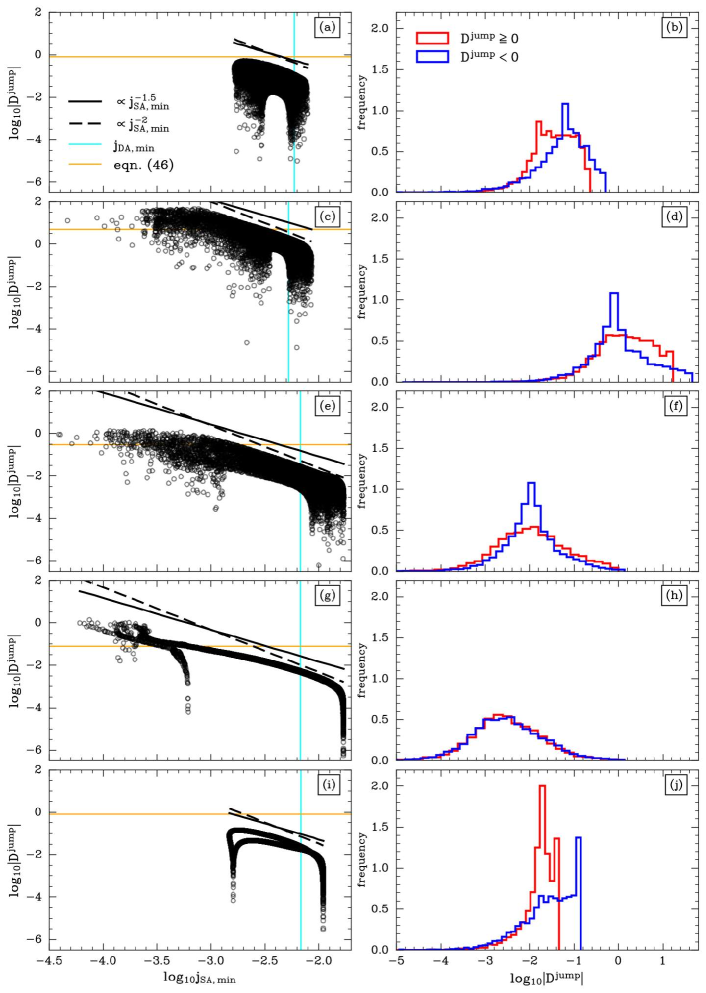
Figure 16.— In panels (a)-(b) we rerun the first secular period from Figure 6, except for $10^{4}$ randomly drawn outer orbital phases, i.e. values of $\phi-\Omega$ and $R$. Panel (a) shows a scatter plot of $|D^{\mathrm{jump}}|$ values from each run against the minimum $j$ value achieved in the SA calculation. Panel (b) shows a histogram of the $|D^{\mathrm{jump}}|$ values from panel (a). Note the initial DA value of $D$ here is $D_{\mathrm{DA}}=-1.036$. Panels (c)-(d) are the same except for the Plummer potential (c.f. Figure 9), with $D_{\mathrm{DA}}=17.624$. Panels (e)-(f) are for the Kepler potential (c.f. Figure 11), with $D_{\mathrm{DA}}=-0.371$. Panels (g)-(h) are again for the Kepler potential as in Figure 11 except we change the outer orbit from $(r_{\mathrm{p}}/b,r_{\mathrm{a}}/b)=(0.7,1.4)$ to $(r_{\mathrm{p}}/b,r_{\mathrm{a}}/b)=(0.7,0.702)$. Panels (i)-(j) are the same except this time we change the outer orbit to $(r_{\mathrm{p}}/b,r_{\mathrm{a}}/b)=(1.4,1.402)$.

In order to probe the statistics of $D^{\mathrm{jump}}$, we first considered an ensemble of $10^{4}$ systems with exactly the same setup and initial conditions as in Figure 6, except in each case we drew a random initial value for $\phi-\Omega$ (uniformly in $(0,2\pi)$) and a random initial radial phase (i.e. for fixed $r_{\mathrm{p}},r_{\mathrm{a}}$ we chose at random the initial radius $R_{0}$, correctly weighted by the time spent at each radius, i.e. $\mathrm{d}N\propto\mathrm{d}R_{0}/v_{R}(r_{\mathrm{p}},r_{\mathrm{a}})$). We stopped each integration at $t\approx t_{\mathrm{sec}}$, i.e. after one full eccentricity oscillation, meaning $D^{\mathrm{jump}}$ was well-established according to equation (46).

The results of this exercise are shown in Figure 16a,b. In panel (a) of this Figure we present a scatter plot of the values of $|D^{\mathrm{jump}}|$ against the minimum $j_{\mathrm{SA}}$ value that was achieved in the corresponding random realization. With a vertical cyan line we show the DA prediction $j_{\mathrm{DA,min}}$, and with a horizontal orange line we show the characteristic estimate (42). In panel (b) we marginalize over $j_{\mathrm{SA,min}}$ in order to produce a histogram of $D^{\mathrm{jump}}$ values, or rather two histograms, one for positive $D^{\mathrm{jump}}$ (red) and one for negative $D^{\mathrm{jump}}$ (blue). From these panels it is clear that there is no very simple dependence of $D^{\mathrm{jump}}$ on $j_{\mathrm{SA,min}}$, nor is there necessarily any symmetry between the distribution of positive and negative $D^{\mathrm{jump}}$ values, nor does the distribution converge to any simple form. In fact, the value of $|D^{\mathrm{jump}}|$ varies over several orders of magnitude, and equation (42) merely provides an estimate (though often not a particularly accurate one) of its maximum value. On the other hand, the upper limit of the envelope of $D^{\mathrm{jump}}$ values is fairly well-fit by a power law $|D^{\mathrm{jump}}|\propto j_{\mathrm{SA,min}}^{-1.5}$ (see the black solid line in panel (a)).

In the remaining panels of Figure 16 we repeat this exercise for several other examples known to exhibit RPSD. In panels (c)-(d) and (e)-(f) respectively we change the potential to the Plummer potential (i.e. taking the initial conditions from Figure 9) and the Kepler potential (taking initial conditions from Figure 11). Again we see that the $|D^{\mathrm{jump}}|$ upper envelopes are fairly well-fit by power laws $|D^{\mathrm{jump}}|\propto j_{\mathrm{SA,min}}^{-1.5}$, but aside from this no robust trend that can be pulled out. Although the histograms of $D^{\mathrm{jump}}$ values in the Kepler case may seem like they have a promising symmetry (panel (f)), this also proves unreliable. To show this, we ran two further examples in the Kepler potential, this time for nearly circular outer orbits. Precisely, in panels (g)-(h) and (i)-(j) we use the same initial conditions as in Figure 11 except we change the outer orbit’s peri/apocenter from $(r_{\mathrm{p}}/b,r_{\mathrm{a}}/b)=(0.7,1.4)$ to $(0.7,0.702)$ and $(1.4,1.402)$ respectively. In these cases, the tracks through $(j_{\mathrm{SA,min}}$, $D^{\mathrm{jump}})$ space approximately follow one-dimensional curves (panels (g) and (i)) rather than a broad two-dimensional distribution, due to the fact that we have removed a degree of freedom (the initial radial phase) by making the outer orbit near-circular. Despite this, there seems to be no simple trend in the distribution of $D^{\mathrm{jump}}$ values (panels (h) and (j)).

In fact, we plotted several such figures for several different sets of initial conditions, cluster potentials, and so on, tried increasing the number of random realizations substantially, and experimented with different ways of binning the values of $D^{\mathrm{jump}}$, but we were unable to uncover any striking insights. We also tried taking the Fourier transform of $\delta j(t)$ near the eccentricity peak and isolating the important frequencies that contribute to the signal, hoping that way to gain insight into RPSD (the same exercise that we performed in panel (r) of Figures 3, (18) and 19). Naturally, we found that these Fourier spectra are concentrated at frequencies $n_{1}\Omega_{R}+n_{2}\Omega_{\phi}$ for pairs of integers $n_{1}$, $n_{2}$ (here $\Omega_{i}\equiv 2\pi/T_{i}$ is the outer orbital frequency). Unfortunately, there were typically several important frequencies at play simultaneously, especially for outer orbits that were far from circular, and we did not extract anything useful from this effort.

5. Discussion

5.1. Astrophysical relevance of RPSD

Since we have uncovered a new effect in this paper the obvious question is: how relevant is it to astrophysical systems? Let us assume that our compact object binary satisfies $\epsilon_{\mathrm{GR}}\ll\epsilon_{\mathrm{weak}}$ and hence reaches very high eccentricity $j_{\mathrm{min}}\sim\Theta^{1/2}$ (Paper III). Assume also that its initial eccentricity is not so large. Then the important necessary condition for significant RPSD to occur is equation (45). In Hamilton & Rafikov (2019a) we considered compact object mergers driven by spherical cluster tides, so we will use that as a test case. There, $10^{7}M_{\odot}$ was the upper limit on sensible cluster masses; $m_{1}=m_{2}=1.4M_{\odot}$ was the lower limit on compact object masses; and $50\mathrm{AU}$ was the upper limit on any sensible distribution of (still rather soft) binaries. Since $\cos i_{0}$ is distributed uniformly $\in(0,1)$ for isotropically oriented binaries, we conclude that RPSD would have affected much less than $1\%$ of our sample. Moreover, this fraction will be even smaller when we consider e.g. BH-BH binaries with $m_{1}=m_{2}=30M_{\odot}$. Thus, we do not expect RPSD to be important for the bulk populations of binary mergers that we considered in Hamilton & Rafikov (2019a).

Nevertheless, it is easy to find numerical examples of compact object binaries orbiting in clusters for which RPSD is a contributing effect (Rasskazov & Rafikov, 2023). In these cases the analytic description of secularly-driven inspirals developed in Hamilton & Rafikov (2022) breaks down completely, and the merger timescale can be wildly different (either longer or shorter) from that used in Hamilton & Rafikov (2019a).

We speculate that RPSD may be important for certain exotic phenomena that involve even more extreme eccentricities, such as head-on collisions of white dwarfs in triple systems (Katz & Dong, 2012). Note that RPSD occurs even for circular outer orbits and for equal mass binaries, i.e. in triples where the octupole contributions to the potential are very small, which are not usually considered promising for producing high merger rates. However, further analysis of this possibility will require incorporating the effects GW emission, which we have neglected throughout this paper. This is left as an avenue for future work.

5.2. Breakdown of the SA approximation

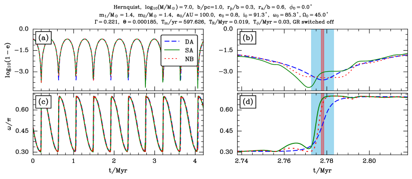
Figure 17.— Example of SA and direct (‘N-body’) integrations disagreeing at high eccentricity. In the right column we zoom in to the seventh eccentricity peak, where the two approaches for calculating $1-e$ disagree by as much as $\sim 0.5$ dex. The blue band in the right hand panels spans $2t_{\mathrm{min}}$ while the red band spans $2T_{\mathrm{in}}$. Note that we started the outer orbit at apocenter, rather than pericenter, in this example.

In this paper we have considered the SA dynamics of binaries driven by cluster tides, particularly at very high eccentricity. We have implicitly assumed that these equations are accurate. It is worth noting, however, that even the SA approximation can itself break down, in situations where any of $(\omega,J,\Omega,J_{z})$ evolve significantly on the timescale of the inner orbital period (Antonini et al., 2014). Such a situation is shown in Figure 17. In this figure we consider a soft NS-NS binary with $T_{\mathrm{in}}\sim 600$ yr, that reaches $1-e\sim 10^{-4}$ in the Hernquist potential. (We do not switch on GR precession in this example, to make it clear that the breakdown of the SA approximation has nothing to do with GR effects). The blue band in the right hand panels spans $2t_{\mathrm{min}}$ while the red band spans $2T_{\mathrm{in}}$. We see that, by the time of the 7th eccentricity peak, the SA result deviates significantly from that found with direct orbit integration, with $1-e$ differing by up to $\sim 0.5$ dex.

Note that the binary component masses are equal in this example, $m_{1}=m_{2}$, so any octupole terms in the tidal force ought to be zero, meaning any corrections are of hexadecapole or higher order. Nevertheless, we checked that the disagreement is really due to a breakdown in the orbit-averaging approximation, rather than these higher order terms, by running a direct orbit integration using the N-body code REBOUND, as in earlier examples, except with the perturbing potential $\Phi(\mathbf{R}_{\mathrm{g}}(t))$ truncated at quadrupole order. The agreement with the full, untruncated direct orbit integration was excellent.

The SA approximation is based on the assumption that $T_{\mathrm{in}}$ is small compared to any other timescale of interest. Thus, the breakdown of the SA approximation occurs if the binary orbital elements, particularly $\omega$ and $\Omega$, change sufficiently rapidly near peak eccentricity, which occurs if $t_{\mathrm{min}}$ is not sufficiently large compared to $T_{\mathrm{in}}$. For instance, in Figure 17, $\omega$ changes by $\sim\pi$ on a timescale of $\sim 5000$ yr. Given $T_{\mathrm{in}}\approx 600$ yr, this corresponds to a rate $\dot{\omega}\sim 20^{\circ}$ per inner orbital period. Such a large value is really an indication that the orbit is not truly Keplerian, and thus that the Keplerian orbital elements themselves are not particularly well-defined; it is perhaps unsurprising that in this regime even the SA approximation breaks down.

5.3. Numerical accuracy

We mention here that in the presence of RPSD, the SA numerical integrations become very expensive, because a very tiny timestep is required in order to get results that are robust over many secular periods. Moreover, any lack of convergence often does not become apparent until late in the integration, when RPSD happens to kick a binary to extremely high eccentricity. For instance, when running the calculation shown in Figure 9, using a slightly larger timestep for the SA integration gave indistinguishable results for the first $\sim 85$ Myr, but during the subsequent high-eccentricity spike there was a noticeable difference in the behavior, after which the two calculations diverged completely. The reason for this divergence is that even tiny errors in the numerical scheme will always accumulate over very long timescales, and will then tend to be amplified during a very high eccentricity episode.

Essentially the same conclusions were recently reached by Rasskazov & Rafikov (2023), who found that because of RPSD the cluster-tide-driven evolution of highly eccentric binaries in the SA approximation (including both GR precession and GW emission) is extremely sensitive to the way in which the cluster tide is computed along the outer orbit.

The difficulty of performing accurate numerical integrations means that for practical purposes, even test-particle, quadrupolar SA evolution may be best thought of as a stochastic process.

5.4. Relation to LK literature

The question of how short-timescale fluctuations affect high eccentricity evolution in LK theory was first addressed by Ivanov et al. (2005), who estimated the amplitude of the angular momentum fluctuations experienced near maximum eccentricity by a binary undergoing LK oscillations. Ivanov et al. (2005)’s result and other results very similar to it have since been used extensively for modelling hierarchical triples (e.g. Katz & Dong 2012; Bode & Wegg 2014; Antognini et al. 2014; Silsbee & Tremaine 2017; Grishin et al. 2018). Their high-$e$ fluctuating torque formula is a special case of our equation (F1). To evaluate this formula, Ivanov et al. (2005) took the outer orbit to be circular; hence our analysis in §F.1 encompasses theirs as a special case. On the other hand, in a Keplerian potential the circular outer orbit approximation is not necessary; Haim & Katz (2018) generalized the result of Ivanov et al. (2005) to eccentric outer orbits. No such generalization is possible for arbitrary spherical cluster potentials.

More recently, as we mentioned in §1.1, Luo et al. (2016) took a perturbative approach to the SA LK problem for arbitrary inner and outer eccentricities. They showed that short-timescale fluctuations captured by the SA equations of motion can accumulate over many secular periods, resulting in secular evolution that does not resemble the original DA prediction. In other words, the time-averaged SA solution does not agree with the DA solution, but instead diverges from it gradually (see Tremaine 2023 for a more rigorous mathematical treatment of this phenomenon). This divergence occurs in a predictable way, and Luo et al. (2016) were able to derive a ‘corrected DA’ Hamiltonian (essentially a ponderomotive potential, see Tremaine 2023) that accurately reproduces the time-averaged SA dynamics. Although Luo et al. (2016) only considered the LK problem up to quadrupolar order in the tidal expansion, their results were generalized to arbitrary (octupole, hexadecapole, …) order by Lei et al. (2018), and then further extended to include fluctuations on the inner orbital timescale $\sim T_{\mathrm{in}}$ by Lei (2019). Moreover, Grishin et al. (2018) applied the formalism of Luo et al. (2016) to high eccentricity behavior (see also Mangipudi et al. 2022). Assuming a circular outer orbit they calculated the new maximum eccentricity arising from Luo et al. (2016)’s ‘corrected’ secular theory, as well as the magnitude of angular momentum fluctuations at highest eccentricity. Though we have not done so here, in the special case of circular outer orbits the results of Luo et al. (2016) and Grishin et al. (2018) could be trivially extended to arbitrary axisymmetric cluster potentials of the sort considered in this paper.

However, in the key papers mentioned above (Ivanov et al., 2005; Luo et al., 2016; Grishin et al., 2018), GR precession was not directly included when calculating the fluctuating behavior at high eccentricity. Those authors also all implicitly assumed the timescale separation $2t_{\mathrm{min}}/T_{\phi}\gg 1$, allowing them to freeze the time-averaged values of $(\omega,J,\Omega,J_{z})$ on the timescale $T_{\phi}$ while they calculated the fluctuations. Our work is different in that we have included GR precession and, crucially, investigated systems with $2t_{\mathrm{min}}/T_{\phi}\lesssim 1$. In this case, the RPSD effect that we have uncovered means that SA dynamics do not converge to the original DA prediction on average, just as was found by Luo et al. (2016) in the non-GR LK theory. However, unlike Luo et al. (2016)’s discovery, RPSD depends critically on the strength of GR precession and also happens very rapidly (on a timescale $t_{\mathrm{min}}\lesssim 2T_{\phi}$) rather than accumulating over many secular periods.

It is also worth contrasting the behavior found in this paper with that from Hamilton & Rafikov (2022). In that case, we found that the secular behavior of binary orbital elements changed over time due to bursts of GW emission at eccentricity peaks, in a purely DA framework — we did not include short-timescale fluctuations. By contrast, in the present paper we have found secular behavior that changes over time due to bursts of RPSD at high eccentricity, which is driven by short-timescale fluctuations and GR precession, but we have not included GW emission. Thus, although we motivated our study by using parameters typical of compact object binaries, in our case the binaries will never merge since there is no dissipation of energy. Since GW emission occurs at a higher (2.5pN) post-Newtonian order than the (1pN) GR precession considered here, we do not expect that it will strongly affect the dynamics of individual RPSD episodes, unless one of those episodes happens to kick the binary into what we called the ‘strong GR regime’ in Hamilton & Rafikov (2022). However, GW emission can certainly make a large difference cumulatively over many secular cycles, as has been recently confirmed by Rasskazov & Rafikov (2023).

Finally, we have considered only quadrupole terms in the tidal potential, i.e. we have considered an SA problem whose DA counterpart is completely integrable (though we note that our direct orbit integrations required no tidal approximation and still provide an excellent match to the SA results). The octupole terms (see Appendix E of Paper I) are very small in most cases we consider, since $a/R$ is very small in applications to binaries in clusters (e.g. Hamilton & Rafikov 2019b). In fact, in all the numerical examples shown in this paper the octupole terms are identically zero, since we always took the binary components to have equal masses $m_{1}=m_{2}$. In LK theory, octupole and higher-order terms are expected to become important when the outer orbit is significantly eccentric and the component masses are not equal, and can lead to non-integrability and hence chaos, both in the SA and DA approximations (Li et al., 2015). We have shown that in the SA approximation, quasi-chaotic phase space behavior can arise even at the pure test particle quadrupole level via RPSD, provided 1PN GR precession is included. Indeed, perhaps the reason that quadrupole-level RPSD has not been mentioned before in the LK literature is that the majority of numerical integrations of the LK equations with GR do include octupolar or higher order terms and/or relax the test-particle approximation, and any complicated behavior that results is then attributed to these effects.

6. Summary

In this paper we have investigated the role of short-timescale fluctuations upon (test particle quadrupole) tide-driven evolution of binary systems, particularly with regard to their high eccentricity behavior. Our main results can be summarized as follows.

• We analyzed the behavior of fluctuations of binary orbital elements in the singly-averaged (SA) approximation, in the absence of 1pN GR apsidal precession. In particular, we derived an expression for the magnitude of angular momentum fluctuations at high eccentricity for binaries orbiting in arbitrary spherically symmetric cluster potentials. Roughly, these fluctuations are comparable in magnitude to the minimum angular momentum predicted by doubly-averaged (DA) theory whenever the cosine of the initial inclination is comparable to or smaller than the ratio of inner and outer orbital periods (equation (28)).

• We then investigated the high eccentricity SA behavior including 1pN GR precession, and found that the evolution can be dramatically different from the case without GR. This can be true even in the weak GR regime (Paper III), where GR makes negligible difference to the DA dynamics. In particular, relativistic phase space diffusion (RPSD) may kick the binary to a new phase space contour on the timescale of the outer orbit, potentially leading to quasi-chaotic evolution and extreme eccentricities, and a full breakdown of the naive DA theory. The rough criterion for RPSD to occur is essentially the same as for angular momentum fluctuations to be comparable to the DA minimum angular momentum (equation (45)), with the additional requirement that GR precession be switched on. The size of the typical RPSD kick is proportional to the dimensionless strength of GR precession $\epsilon_{\mathrm{GR}}$.

• RPSD likely affects only a very small fraction of binaries in population synthesis studies of LIGO/Virgo gravitational wave sources, but may be a crucial ingredient for e.g. head-on collisions of white dwarfs.

Appendix A Singly-averaged equations of motion in the test-particle, quadrupole limit for arbitrary cluster potentials

The full SA Hamiltonian is $H_{\mathrm{SA}}=H_{\mathrm{1,SA}}+H_{\mathrm{GR}}$ where $H_{\mathrm{GR}}$ is given by (10) and $H_{1,\mathrm{SA}}$ is given by (8). The corresponding SA equations of motion are

$$\frac{\mathrm{d}\omega}{\mathrm{d}t}= \frac{\partial H_{\mathrm{1,SA}}}{\partial J}+\frac{\partial H_{\mathrm{GR}}}{\partial J}$$

$$= [L^{2}/(8J^{4}\mu^{2})]\times$$

$$\Bigg{\{}(\Phi_{xx}+\Phi_{yy})\Big{[}-J^{5}(3+5\cos 2\omega)-5JJ_{z}^{2}L^{2}(1-\cos 2\omega)\Big{]}$$

$$+(\Phi_{xx}-\Phi_{yy})\Big{[}-J^{5}(3+5\cos 2\omega)\cos 2\Omega+5JJ_{z}^{2}L^{2}(1-\cos 2\omega)\cos 2\Omega+5J^{2}J_{z}(J^{2}+L^{2})\sin 2\Omega\sin 2\omega\Big{]}$$

$$+\Phi_{zz}\Big{[}-6J^{5}+10JJ_{z}^{2}L^{2}+10(J^{5}-JJ_{z}^{2}L^{2})\cos 2\omega\Big{]}$$

$$+\Phi_{xy}\Big{[}-10J^{2}J_{z}(J^{2}+L^{2})\cos 2\Omega\sin 2\omega-J^{5}\sin 2\Omega(6+10\cos 2\omega)+10JJ_{z}^{2}L^{2}\sin 2\Omega(1-\cos 2\omega)\Big{]}$$

$$+\Phi_{xz}(1-J_{z}^{2}/J^{2})^{-1/2}\Big{[}J_{z}(6J^{4}+10J^{2}L^{2}-20J_{z}^{2}L^{2})\sin\Omega$$

$$+J(-20J^{4}+10J^{2}J_{z}^{2}+10J_{z}^{2}L^{2})\sin 2\omega\cos\Omega+J_{z}(-10J^{4}-10J^{2}L^{2}+20J_{z}^{2}L^{2})\cos 2\omega\sin\Omega\Big{]}$$

$$+\Phi_{yz}(1-J_{z}^{2}/J^{2})^{-1/2}\Big{[}-J_{z}(6J^{4}+10J^{2}L^{2}-20J_{z}^{2}L^{2})\cos\Omega$$

$$+J(-20J^{4}+10J^{2}J_{z}^{2}+10J_{z}^{2}L^{2})\sin 2\omega\sin\Omega-J_{z}(-10J^{4}-10J^{2}L^{2}+20J_{z}^{2}L^{2})\cos 2\omega\cos\Omega\Big{]}\Bigg{\}}+\frac{AL^{5}\epsilon_{\mathrm{GR}}}{8\mu^{2}J^{2}},$$ (A1)

$$\frac{\mathrm{d}J}{\mathrm{d}t}= -\frac{\partial H_{\mathrm{1,SA}}}{\partial\omega}$$

$$= [5L^{2}/(2J^{2}\mu^{2})](J^{2}-L^{2})\times$$

$$\Bigg{\{}-0.25(\Phi_{xx}+\Phi_{yy})\Big{[}(J^{2}-J_{z}^{2})\sin 2\omega\Big{]}-0.25(\Phi_{xx}-\Phi_{yy})\Big{[}(J^{2}+J_{z}^{2})\cos 2\Omega\sin 2\omega+2JJ_{z}\cos 2\omega\sin 2\Omega\Big{]}$$

$$+\Phi_{zz}\Big{[}0.5(J^{2}-J_{z}^{2})\sin 2\omega\Big{]}+\Phi_{xy}\Big{[}JJ_{z}\cos 2\omega\cos 2\Omega-0.5(J^{2}+J_{z}^{2})\sin 2\omega\sin 2\Omega\Big{]}$$

$$+\Phi_{xz}\Big{[}J\sqrt{1-J_{z}^{2}/J^{2}}(J\cos 2\omega\cos\Omega-J_{z}\sin 2\omega\sin\Omega)\Big{]}+\Phi_{yz}\Big{[}J\sqrt{1-J_{z}^{2}/J^{2}}(J\cos 2\omega\sin\Omega+J_{z}\sin 2\omega\cos\Omega)\Big{]}\Bigg{\}},$$ (A2)

$$\frac{\mathrm{d}\Omega}{\mathrm{d}t}= \frac{\partial H_{\mathrm{1,SA}}}{\partial J_{z}}$$

$$= [L^{2}/(4J^{3}\mu^{2})]\times$$

$$\Bigg{\{}(\Phi_{xx}+\Phi_{yy})\Big{[}0.5JJ_{z}(-3J^{2}+5L^{2}+5(J^{2}-L^{2})\cos 2\omega)\Big{]}$$

$$+(\Phi_{xx}-\Phi_{yy})\Big{[}-0.5JJ_{z}\cos 2\Omega(-3J^{2}+5L^{2}+5(J^{2}-L^{2})\cos 2\omega)+5J^{2}(J^{2}-L^{2})\sin 2\omega\sin 2\Omega]\Big{]}$$

$$-\Phi_{zz}\Big{[}JJ_{z}(-3J^{2}+5L^{2}+5(J^{2}-L^{2})\cos 2\omega)\Big{]}$$

$$-\Phi_{xy}\Big{[}J[5J(J^{2}-L^{2})\cos 2\Omega\sin 2\omega+J_{z}(-3J^{2}+5L^{2}+5(J^{2}-L^{2})\cos 2\omega)\sin 2\Omega]\Big{]}$$

$$+\Phi_{xz}(1-J_{z}^{2}/J^{2})^{-1/2}\Big{[}5JJ_{z}(J^{2}-L^{2})\sin 2\omega\cos\Omega$$

$$+[3J^{4}+10J_{z}^{2}L^{2}+J^{2}(-6J_{z}^{2}-5L^{2})+(-5J^{4}-10J_{z}^{2}L^{2}+J^{2}(10J_{z}^{2}+5L^{2}))\cos 2\omega]\sin\Omega\Big{]}$$

$$+\Phi_{yz}(1-J_{z}^{2}/J^{2})^{-1/2}\Big{[}5JJ_{z}(J^{2}-L^{2})\sin 2\omega\sin\Omega$$

$$-[3J^{4}+10J_{z}^{2}L^{2}+J^{2}(-6J_{z}^{2}-5L^{2})+(-5J^{4}-10J_{z}^{2}L^{2}+J^{2}(10J_{z}^{2}+5L^{2}))\cos 2\omega]\cos\Omega\Big{]}\Bigg{\}},$$ (A3)

$$\frac{\mathrm{d}J_{z}}{\mathrm{d}t}= -\frac{\partial H_{\mathrm{1,SA}}}{\partial\Omega}$$

$$= -[L^{2}/(4J^{2}\mu^{2})]\times$$

$$\Bigg{\{}(\Phi_{xx}-\Phi_{yy})\Big{[}5JJ_{z}(J^{2}-L^{2})\cos 2\Omega\sin 2\omega+0.5((J^{2}-J_{z}^{2})(3J^{2}-5L^{2})+5(J^{2}+J_{z}^{2})(J^{2}-L^{2})\cos 2\omega)\sin 2\Omega\Big{]}$$

$$+\Phi_{xy}\Big{[}((-J^{2}+J_{z}^{2})(3J^{2}-5L^{2})-5(J^{2}+J_{z}^{2})(J^{2}-L^{2})\cos 2\omega)\cos 2\Omega+10JJ_{z}(J^{2}-L^{2})\sin 2\omega\sin 2\Omega\Big{]}$$

$$-\Phi_{xz}\Big{[}J\sqrt{1-J_{z}^{2}/J^{2}}(-5J(J^{2}-L^{2})\sin\Omega\sin 2\omega+J_{z}(-3J^{2}+5L^{2}+5(J^{2}-L^{2})\cos 2\omega)\cos\Omega)\Big{]}$$

$$-\Phi_{yz}\Big{[}J\sqrt{1-J_{z}^{2}/J^{2}}(5J(J^{2}-L^{2})\cos\Omega\sin 2\omega+J_{z}(-3J^{2}+5L^{2}+5(J^{2}-L^{2})\cos 2\omega)\sin\Omega)\Big{]}\Bigg{\}}.$$ (A4)

In the case of axisymmetric cluster potentials, it is straightforward to recover the DA equations from the SA equations (A)-(A) by replacing the time-dependent quantities $\Phi_{\alpha\beta}$ with their time-averages $\overline{\Phi}_{\alpha\beta}$, and using the identities $\overline{\Phi}_{xx}=\overline{\Phi}_{yy}$ and $\overline{\Phi}_{xy}=\overline{\Phi}_{xz}=\overline{\Phi}_{yz}=0$ (see equations (33)-(36) of Paper I).

Appendix B A note on phase space morphology

The phase space trajectories described by the DA Hamiltonian (9) fall into two categories — librating trajectories, which loop around fixed points at $\omega=\pm\pi/2$ in the $(\omega,j)$ phase plane, and circulating trajectories, which traverse all $\omega\in(-\pi,\pi)$. Whether a binary’s trajectory will librate or circulate depends on its initial orbital elements as well as the value of $\Gamma$. In Paper II we showed how to determine the family to which a binary’s phase space trajectory belongs, explained how this affects the resulting minimum/maximum eccentricity achievable, etc. We also explained there how altering $\Gamma$ changes the phase space morphology, and hence the relative importance of librating versus circulating trajectories. In particular, $\Gamma=0,\pm 1/5$ turn out to be critical values, such that e.g. systems with $\Gamma>1/5$ have a qualitatively different phase space morphology to those with $0<\Gamma<1/5$, a result which has strong implications for the types of cluster which are able to easily excite high eccentricity behavior (Hamilton & Rafikov, 2019a, 2022). Moreover, In Paper III we extended these results to include the effect of GR precession, which also alters the phase space morphology.

However, for the purposes of studying short-timescale fluctuations at extremely high eccentricity, it is largely irrelevant whether a binary is on a librating or circulating trajectory, or which $\Gamma$ regime it happens to be in. This is because the details of the high eccentricity fluctuations depend predominantly on very short short-timescale (of order the outer orbital period $\sim T_{\phi}$) torquing that the binary experiences as $e\to 1$, and not on the averaged behavior over the rest of the secular cycle. For instance, the numerical examples we present in this paper all happen to be for librating trajectories, but we have found qualitatively indistinguishable results for circulating examples. Similarly, we do show examples with both $\Gamma>1/5$ and $0<\Gamma<1/5$ in this paper, but the distinction between these two $\Gamma$ regimes is not central to our discussion, so we mostly neglect to mention it in the main text.

Appendix C Additional numerical examples of high eccentricity behavior without GR precession

C.1. Changing the initial inclination to $i_{0}=93.3^{\circ}$

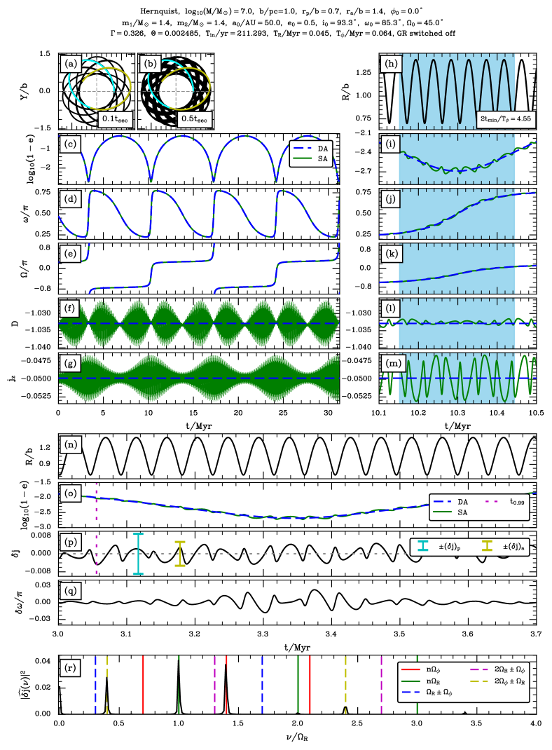
Figure 18.— As in Figure 3 except we change $i_{0}$ to $93.3^{\circ}$. As a result $e_{\mathrm{max}}$ is decreased and $2t_{\mathrm{min}}$ becomes significantly larger than $T_{\phi}$. The DA secular period is again $t_{\mathrm{sec}}\approx 6.9$ Myr.

In Figure 18 we run the same calculation as in Figure 3, except we take $i_{0}=93.3^{\circ}$ rather than $90.3^{\circ}$. The main effect of this choice is to reduce the maximum eccentricity significantly, so that $1-e_{\mathrm{max}}\approx 10^{-2.7}$. As a result, DA evolution near maximum eccentricity is slower than in Figure 3, while the outer orbit is unchanged; hence we find $2t_{\mathrm{min}}/T_{\phi}=4.55$ in this case. The qualitative fluctuating behavior of $D$, $j_{z}$ and $\delta j$ is quite similar between the two figures, although in Figure 18 many more fluctuations fit into the ‘blue stripe’ surrounding maximum eccentricity. The fluctuations $\delta\omega$ are very different: the brief ‘pulse’ that lasted for only $\sim 2T_{R}$ in Figure 3q has been replaced with a much broader signal with a slightly smaller amplitude.

C.2. An example in the Plummer potential

The phenomenology reported above is rather characteristic of binaries orbiting in cusped potentials, and will be analysed more quantitatively in §3.2. First, however, we perform the same calculation except this time with a cored potential, namely the Plummer sphere.

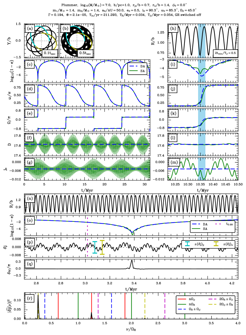
Figure 19.— As in Figure 3, except this time we use the Plummer potential. Here $t_{\mathrm{sec}}\approx 7.0$ Myr.

Figure 20.— Plotting the inclination $i=\arccos(j_{z}/j)$ around the first eccentricity peak from Figure 19. The SA result reveals that near peak eccentricity, the binary experiences orbital ‘flips’ whereby its inclination crosses $90^{\circ}$.

In Figure 19 we provide an example of a binary exhibiting short-timescale fluctuations in a cored potential. All input parameters are the same as in Figure 3 except we change the potential from Hernquist to Plummer, so $\Phi=-G\mathcal{M}/\sqrt{b^{2}+r^{2}}$ (we again use $\mathcal{M}=10^{7}M_{\odot}$ and $b=1$pc). The change of potential means that we now have $\Gamma=0.194<1/5$, which leads to a rather large $D_{\mathrm{DA}}$ value of around $17.6$ (equation (13)).

Noteworthy in this case is the morphology of the fluctuations of $j_{z,\mathrm{SA}}$ near highest eccentricity, around the DA value $j_{z,\mathrm{DA}}=-\sqrt{\Theta}=-0.0045$ (panel (m)). In this case, small oscillations on the timescale $\sim T_{R}$ are superimposed upon a larger ‘carrier signal’ oscillation, which has amplitude $\sim 0.006$ and its own period $\sim 4T_{R}$. In this case these fluctuations can actually change the sign of $j_{z}$, which corresponds to the SA binary inclination $i$ temporarily passing through $90^{\circ}$, a so-called ‘orbital flip’ — see Naoz (2016); Grishin et al. (2018). In Figure 20 we show the inclination $i(t)$ explicltly for SA and DA integrations; we see that near peak eccentricity the DA approximation fails entirely to capture the flip behavior.

A similar morphology is exhibited by the $\delta j$ time series (panel (p)). Again the fluctuations $\delta\omega$ (panel (q)) are negligible until the very highest eccentricities are reached, where there is a sharp, negative pulse of maximum amplitude $\sim 0.2\pi$, that lasts for $\sim 2T_{R}$ in total before decaying back to zero.

C.3. Dependence on phase angles

It is also worth emphasising here the dependence of these results on the choice of various phase angles, namely the initial radial phase of the outer orbit, the initial azimuthal angle of the outer orbit $\phi$, and the initial choice of longitude of ascending node $\Omega$ of the inner orbit. These choices feed into the solutions of the SA equations of motion (A1)-(A4), though of course they do not affect the DA solutions. By inspecting numerical examples without GR precession (such as that in Figure 1, as well as several others not shown here), we found that the choice of these phase angles can significantly affect e.g. the maximum value of $e_{\mathrm{SA}}$ that is reached by a binary, but that the qualitative behavior is very similar from one realization to the next, and the averaged values of $D$ and $j_{z}$ are conserved. However, this ceases to be true when GR precession is included, as we saw in Figure 2 (see also §4).

Appendix D Fluctuating Hamiltonian

By subtracting the DA Hamiltonian from the SA Hamiltonian, assuming them to be functions of the same variables $(J,\omega,...)$, and using $\Phi_{xx}=\overline{\Phi}_{yy}$ and $\overline{\Phi}_{xy}=\overline{\Phi}_{xz}=\overline{\Phi}_{yz}=0$, we get an expression for the ‘fluctuating Hamiltonian’ (equation (19)):

$$\Delta H\equiv H_{\mathrm{SA}}(J,\omega,...)-H_{\mathrm{DA}}(J,\omega,...)=\frac{1}{2}\sum_{\alpha\beta}(\Phi_{\alpha\beta}(t)-\overline{\Phi}_{\alpha\beta})\langle r_{\alpha}r_{\beta}\rangle_{M}$$

$$= \frac{1}{2}\Bigg{\{}(\Phi_{xx}-\overline{\Phi}_{xx})\langle x^{2}\rangle_{M}+(\Phi_{yy}-\overline{\Phi}_{xx})\langle y^{2}\rangle_{M}+(\Phi_{zz}-\overline{\Phi}_{zz})\langle z^{2}\rangle_{M}+\Phi_{xy}\langle xy\rangle_{M}+\Phi_{xz}\langle xz\rangle_{M}+\Phi_{yz}\langle yz\rangle_{M}\Bigg{\}}.$$ (D1)

(Note that the term involving $\epsilon_{\mathrm{GR}}$ has disappeared, since it is the same in SA and DA theory). Equation (D1) holds for binaries in arbitrary axisymmetric potentials.

We can simplify matters significantly if we restrict ourselves to spherical potentials $\Phi(r)=\Phi(\sqrt{R^{2}+Z^{2}})$. Let us define

$$f_{\pm}(\mathbf{R}_{\mathrm{g}}(t))\equiv\frac{1}{2}\left[\left(\frac{\partial^{2}\Phi}{\partial R^{2}}\right)_{\mathbf{R}_{\mathrm{g}}}\pm\left(\frac{1}{R}\frac{\partial\Phi}{\partial R}\right)_{\mathbf{R}_{\mathrm{g}}}\right],$$ (D2)

and assume without loss of generality that $\mathbf{R}_{\mathrm{g}}$ is confined to $Z=0$. Then it is easy to show (see equations (33)-(36) of Paper I) that:

$$\Phi_{xx}=f_{+}+f_{-}\cos 2\phi,\,\,\,\,\,\,\,\,\,\Phi_{yy}=f_{+}-f_{-}\cos 2\phi,\,\,\,\,\,\,\,\,\,\Phi_{zz}=f_{+}-f_{-},\,\,\,\,\,\,\,\,\,\,\,\Phi_{xy}=f_{-}\sin 2\phi,\,\,\,\,\,\,\,\,\,\,\Phi_{xz}=\Phi_{yz}=0.$$ (D3)

(Note that we have dropped the ‘g’ subscript for ease of notation). If we also define $\Delta f_{\pm}\equiv f_{\pm}-\overline{f}_{\pm}$ where $\overline{f}_{\pm}$ is the annulus-averaged value of $f_{\pm}$ then the fluctuating Hamiltonian can be written concisely as

$$\Delta H= \frac{1}{2}\left[\Delta f_{+}\langle x^{2}+y^{2}+z^{2}\rangle_{M}-\Delta f_{-}\langle z^{2}\rangle_{M}+f_{-}\left(\langle x^{2}-y^{2}\rangle_{M}\cos 2\phi+2\langle xy\rangle_{M}\sin 2\phi\right)\right].$$

$$= \frac{L^{2}}{8J^{2}\mu^{2}}\Bigg{\{}(3J^{2}-5L^{2})\Big{[}(\Delta f_{-}-2\Delta f_{+})J^{2}-\Delta f_{-}J_{z}^{2}+f_{-}(-J^{2}+J_{z}^{2})\cos[2(\Omega-\phi)]\Big{]}$$

$$-5(J^{2}-L^{2})\cos 2\omega\Big{[}\Delta f_{-}(J^{2}-J_{z}^{2})+f_{-}(J^{2}+J_{z}^{2})\cos[2(\Omega-\phi)]\Big{]}+10f_{-}JJ_{z}(J^{2}-L^{2})\sin 2\omega\sin[2(\Omega-\phi)]\Bigg{\}}.$$ (D4)

As explained in §3.2, equations for the evolution of fluctuations in orbital elements be derived from the fluctuating Hamiltonian $\Delta H(\omega,J,..)$ by taking its partial derivatives (equation (21)). In particular, we have

$$\frac{\partial\Delta H}{\partial\omega} =\frac{5}{4}\frac{L^{2}}{J^{2}\mu^{2}}(J^{2}-L^{2})\Bigg{\{}\sin 2\omega(J^{2}-J_{z}^{2})\Delta f_{-}+f_{-}\Big{(}(J^{2}+J_{z}^{2})\sin 2\omega\cos[2(\phi-\Omega)]-2JJ_{z}\cos 2\omega\sin[2(\phi-\Omega)]\Big{)}\Bigg{\}}.$$ (D5)

Assuming this to be a good approximation to $-\mathrm{d}\delta j/\mathrm{d}t$ at high $e$, as we do in §3.3, it constitutes a generalisation of equation (B4) of Ivanov et al. (2005). The result of Ivanov et al. (2005) is recovered if one assumes the outer orbit to be circular (so $\Delta f_{\pm}=0$), the perturbing potential to be Keplerian, and evaluates (D5) at $\omega=\pm\pi/2$ and $e\to 1$. We also have

$$\frac{\partial\Delta H}{\partial\Omega}= \frac{L^{2}}{4J^{2}\mu^{2}}f_{-}\Bigg{\{}10JJ_{z}(J^{2}-L^{2})\sin 2\omega\cos[2(\phi-\Omega)]$$

$$-((J^{2}-J_{z}^{2})(3J^{2}-5L^{2})+5(J^{2}+J_{z}^{2})(J^{2}-L^{2})\cos 2\omega)\sin[2(\phi-\Omega)]\Bigg{\}},$$ (D6)

which coincides precisely with (minus) the right hand side of (A4) if one assumes $\Phi$ to be spherical. This is as it must be, since in DA dynamics $J_{z}$ is perfectly conserved, and so $\mathrm{d}J_{z}/\mathrm{d}t=\mathrm{d}\delta J_{z}/\mathrm{d}t$, as we argued below equation (E1).

Appendix E Justifying the approximation $\delta\mathbf{w}\approx\Delta\mathbf{w}(\mathbf{w}_{\mathrm{SA}})\approx\Delta\mathbf{w}(\mathbf{w}_{\mathrm{DA}})$

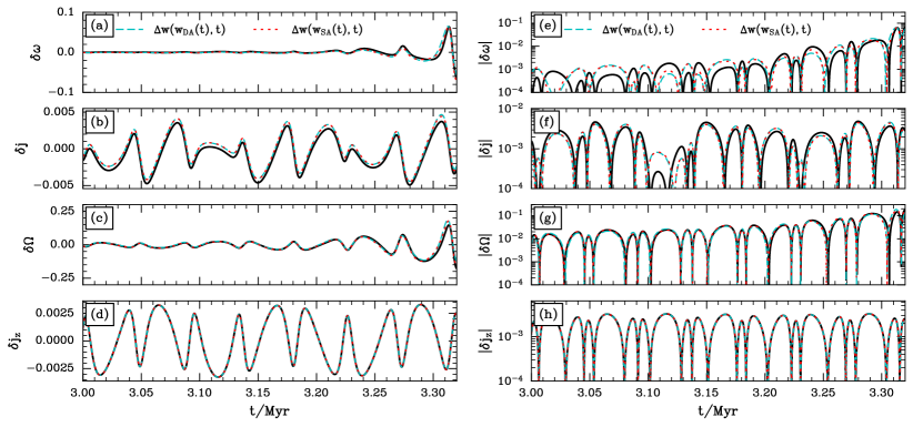
Figure 21.— Justifying the approximation $\delta\mathbf{w}(t)\approx\Delta\mathbf{w}(\mathbf{w}_{\mathrm{SA}},t)\approx\Delta\mathbf{w}(\mathbf{w}_{\mathrm{DA}},t)$. In panels (a)-(d), black solid lines show the evolution of $\delta\bm{\mathbf{w}}\equiv\mathbf{w}_{\mathrm{SA}}-\mathbf{w}_{\mathrm{DA}}$ using the data from Figure 3 during the time interval $t\in(3,3.32)$Myr (the first peak in DA eccentricity occurs at $t\approx 3.34$Myr). Cyan dashed lines and red dotted lines show the approximations $\Delta\mathbf{w}(\mathbf{w}_{\mathrm{SA}},t)$ and $\Delta\mathbf{w}(\mathbf{w}_{\mathrm{SA}},t)$ respectively. In panels (e)-(h) we show the same data using a logarithmic scale.

If we feed a numerical result $\mathbf{w}(t)=\mathbf{w}_{\mathrm{SA}}(t)$ into equation (21) and integrate forwards in time, we do not in general reproduce the ‘SA minus DA’ solution (18); for example:

$$\delta\omega(t) \equiv\omega_{\mathrm{SA}}(t)-\omega_{\mathrm{DA}}(t)$$

$$\neq\Delta\omega(\mathbf{w}_{\mathrm{SA}}(t),t)\equiv\int_{0}^{t}\mathrm{d}t^{\prime}\frac{\partial\Delta H(\mathbf{w}_{\mathrm{SA}}(t^{\prime}),t^{\prime})}{\partial J_{\,\mathrm{SA}}}.$$ (E1)

Similarly, $\delta J\neq\Delta J$ and $\delta\Omega\neq\Delta\Omega$. The exception is $J_{z}$, for which there is no DA evolution, so that $\delta J_{z}(t)=\Delta J_{z}(\mathbf{w}_{\mathrm{SA}}(t),t)$. We feel it is important to make this distinction since it affects perturbative calculations — for example, Luo et al. (2016) implicitly used $\delta\mathbf{w}(t)=\Delta\mathbf{w}(\mathbf{w}_{\mathrm{DA}}(t),t)$ when calculating the cumulative impact of short-timescale fluctuations over many secular cycles, by ‘freezing’ the DA elements on the timescale of the outer orbit. See §5.4 for more.

Nevertheless, these quantities are approximately equal, as we wrote in equation (23). There are two basic reasons why this approximation holds. The first is that the torques felt by an extremely eccentric binary are not particularly sensitive to its exact orbital elements. For instance, the torque on a binary at $e_{\mathrm{DA}}=0.999$ is not particularly different from that on a binary with $e_{\mathrm{SA}}=0.9995$, since in each case the inner-orbit-averaged version of that binary essentially looks like a one-dimensional line. Second, there is a sensitive dependence of the precession of $\omega$ and $\Omega$ upon the exact value of eccentricity as $e\to 1$ (see equation (24)), but the high-$e$ episode is over so quickly that this does not lead to a significant breakdown of equation (23).

To demonstrate the accuracy of the approximation (23), we took the quantities from Figure 4 and integrated them forwards in time using (21). We plot the result in Figure 21 on top of the ‘true’ fluctuation $\delta\mathbf{w}(t)$, shown with black lines. We see that the approximation (23) works very well in this case; we also confirmed its accuracy in several other examples not shown here, including in cases with GR precession switched on (relevant for §4).

Appendix F Characteristic amplitude of angular momentum fluctuations

For simplicity we will assume that $\Phi$ is spherically symmetric. Then to evaluate the torque at high eccentricity we can use (D5), which by (21) and (23) is a good approximation to $-\mathrm{d}\delta j/\mathrm{d}t$ if we evaluate it using DA quantities. The maximum eccentricity as predicted by the DA theory is $e_{\mathrm{DA}}=e_{\mathrm{max}}\approx 1$, and it always occurs either at $\omega_{\mathrm{DA}}=\pm\pi/2$ or at $\omega_{\mathrm{DA}}=0$. Let the corresponding minimum inclination be $i_{\mathrm{min}}$. Evaluating (D5) at these (assumed fixed) DA values, we find

$$\frac{\mathrm{d}\delta J}{\mathrm{d}t}\bigg{|}_{\omega=\pm\pi/2}= \frac{5}{4}a^{2}\cos i_{\mathrm{min}}\times 2f_{-}(R)\sin[2(\phi-\Omega)],$$ (F1)

or the same thing with an additional minus sign if evaluating at $\omega=0$. Note that the function $f_{-}(R)$, defined in equation (D2), depends on the instantaneous value of the outer orbital radius $R(t)$. Finally, one can check that for a Keplerian potential $\Phi=-G\mathcal{M}/R$ we recover equation (B4) of Ivanov et al. (2005).

Next we use the fact that in DA theory $i_{\mathrm{min}}$ does not vary from one eccentricity peak to the next, and we assume that $\Omega_{\mathrm{DA}}$ is stationary on the timescale $T_{\phi}$. (This assumption, along with that of stationary $\omega_{\mathrm{DA}}$ and $e_{\mathrm{DA}}$ on the timescale $T_{\phi}$, breaks down whenever $t_{\mathrm{min}}\lesssim T_{\phi}$ — see Figures 3, (18) and 19, as well as Appendix C of Paper III. Nevertheless, these assumptions are good enough in order to get for a simple estimate of $(\delta j)_{\mathrm{max}}$ which is all we need here). Placing the maximum DA eccentricity at $t=0$ without loss of generality, we set $\Omega=\Omega(0)$. Then the only time dependence in equation (F1) comes from $R(t)$ and $\phi(t)$. Furthermore, $f_{-}(R)<0$ for all $R$ in sensible cluster potentials. As a result, the sign of the torque at highest eccentricity (equation (F1)) is dictated entirely by the instantaneous value of the phase angle $2(\phi-\Omega)$. The fluctuation $(\delta j)_{\mathrm{max}}$ is therefore accumulated over a quarter period in azimuth, say from $\phi(t_{1})-\Omega=0$ to $\phi(t_{2})-\Omega=\pi/2$, after which the torque changes sign. Integrating (F1) over time we find

$$(\delta j)_{\mathrm{max}} =\frac{5}{4}\left[\frac{a^{3}}{G(m_{1}+m_{2})}\right]^{1/2}\cos i_{\mathrm{min}}\,F(r_{\mathrm{p}},r_{\mathrm{a}})$$ (F3)

$$= 10^{-4}\times\left(\frac{\sqrt{\Theta}/j_{\mathrm{min}}}{1}\right)\left(\frac{m_{1}+m_{2}}{M_{\odot}}\right)^{-1/2}\left(\frac{a}{10\mathrm{AU}}\right)^{3/2}\left(\frac{F^{*}}{0.8}\right)\left(\frac{M}{10^{5}M_{\odot}}\right)^{1/2}\left(\frac{b}{\mathrm{pc}}\right)^{-3/2},$$ (F4)

where all the details of the potential and outer orbit have been absorbed by the function

$$F(r_{\mathrm{p}},r_{\mathrm{a}})=\int_{t_{1}}^{t_{2}}\mathrm{d}t\,\left|\frac{\partial^{2}\Phi}{\partial R^{2}}-\frac{1}{R}\frac{\partial\Phi}{\partial R}\right|\,\sin[2(\phi-\Omega)],$$ (F5)

and in the numerical estimate (F4) we defined the dimensionless number

$$F^{*}\equiv\left(\frac{G\mathcal{M}}{b^{3}}\right)^{-1/2}F.$$ (F6)

F.1. Circular outer orbits

The simplest (and practically speaking, only) way to proceed more quantitatively than this is to estimate $F$ by imagining that the binary is on a circular outer orbit with radius $R$. Then $F=F_{\mathrm{circ}}(R)$ where

$$F_{\mathrm{circ}}(R) =2\Omega_{\mathrm{circ}}\Bigg{|}\frac{\partial\ln\Omega_{\mathrm{circ}}}{\partial\ln R}\Bigg{|},$$ (F7)

where $\Omega_{\mathrm{circ}}(R)=[R^{-1}\partial\Phi/\partial R]^{1/2}$ is the angular frequency of a circular orbit of radius $R$. In the LK case of Keplerian potentials, the result arising from (F3) with the circular approximation (F7) was already derived by Ivanov et al. (2005).

In Figure 22 we plot the dimensionless number $F_{\mathrm{circ}}^{*}\equiv(G\mathcal{M}/b^{3})^{-1/2}F_{\mathrm{circ}}$ as a function of $R/b$ for circular outer orbits in various spherically symmetric cluster potentials with scale radius $b$. For reference we also plot $F_{\mathrm{circ}}^{*}$ for the Kepler potential $\Phi=-G\mathcal{M}/R$.

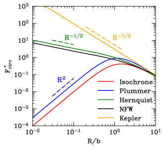
Figure 22.— Plot of the dimensionless function $F_{\mathrm{circ}}^{*}\equiv F_{\mathrm{circ}}(R)/(G\mathcal{M}/b^{3})^{1/2}$, where $F$ is defined in equation (F7), for four spherical potentials with scale radius $b$, as well as the Kepler potential $\Phi=-G\mathcal{M}/r$.

We see that in the cored (Plummer and isochrone) models $F_{\mathrm{circ}}^{*}$ has a maximum value of order unity which is realised when $R\sim b$, and that it falls sharply to zero towards the centre of the cluster. For centrally cusped potentials (Hernquist and NFW) we again have $F_{\mathrm{circ}}^{*}\sim 1$ at intermediate radii $R\sim b$, but $F_{\mathrm{circ}}^{*}$ diverges towards the centre as $\sim R^{-1/2}$, typically reaching $F_{\mathrm{circ}}^{*}\sim 10$ at the smallest sensible radii. At very large radii $R\gg b$, the isochrone, Plummer and Hernquist potentials tend toward Keplerian behavior, $F_{\mathrm{circ}}^{*}\sim R^{-3/2}$. (The logarithm in the NFW potential means it never quite becomes Keplerian at these radii).

From Figure 22 we learn that (i) the magnitude of short-timescale angular momentum fluctuations is roughly independent of potential type for $R\gtrsim b$, (ii) short-timescale fluctuations are significantly larger in cusped potentials than in cored potentials for $R<b$, and (iii) very large values of $F^{*}$ can be reached at small radii in the Kepler potential.

F.2. Further discussion and examples

Although it is strictly valid for circular outer orbits only, Figure 22 can also teach us something about non-circular outer orbits. For instance, in cusped potentials, the scaling of $F_{\mathrm{circ}}^{*}$ with $R$ suggests that as long as the outer orbit is not too eccentric, a decent approximation to the dominant short-timescale fluctuation can be found by employing the circular approximation with $F_{\mathrm{circ}}$ (equation (F7)) evaluated at $R=r_{\mathrm{p}}$. In cored potentials this is no longer true because of the turnover in $F_{\mathrm{circ}}^{*}$ at $R\sim b$. Then, for example, for orbits with $r_{\mathrm{a}}\lesssim b$ the dominant $j$ fluctuations clearly arise around apocenter passage, since this is where $F_{\mathrm{circ}}^{*}$ is largest and this is where the outer orbit spends the most time. However, outer orbits in cored potentials with $r_{\mathrm{a}}\lesssim b$ tend to have $\Gamma<1/5$ (Paper I), so they tend not to reach such high eccentricities anyway, and besides, the values of $F_{\mathrm{circ}}^{*}$ never exceeds $\sim 1$ regardless of $R$ for these potentials. Hence, for an order of magnitude estimate we may choose simply to evaluate $(\delta j)_{\mathrm{max}}$ using equation (F7) with $R=r_{\mathrm{p}}$, regardless of the type of potential or outer orbit.

In panel (p) of Figures 3 and 19 we show as ‘error bars’ the values of $\pm(\delta j)_{\mathrm{p}}$ (cyan) and $\pm(\delta j)_{\mathrm{a}}$ (yellow), which are calculated by evaluating $\pm(\delta j)_{\mathrm{max}}$ (equation (F3)) using the circular approximation (F7) at $R=r_{\mathrm{p}}$ and $R=r_{\mathrm{a}}$ respectively. We see that the circular approximation gives a reasonable estimate of the amplitude of fluctuations $\delta j$.

One important caveat here is that while the $\delta j(t)$ behavior is often rather regular up to $e_{\mathrm{DA}}\lesssim 0.99$, it often becomes rather irregular in the immediate vicinity of the eccentricity peak, as can be seen in Figures 3 and 19. This is because of the rapid evolution, $\omega$, $\Omega$ and $i$ when $j\approx j_{\mathrm{min}}$ (see the light blue shaded bands in panels (j) and (k) of each of those Figures, as well as the inclination plot in Figure 20) which introduces a significant phase dependence into the detailed fluctuation behavior. Of course, since (F3) was derived by assuming stationary $\omega,\Omega,i,j$, it necessarily fails to capture this irregular behavior.

Finally, we attempted to capture the complicated behavior of $\delta j(t)$ near the eccentricity peak for non-circular outer orbits, and thereby move beyond the circular approximation, by isolating the contribution of individual Fourier modes $\widehat{\delta j}(\nu)$ (panel (r) of Figures 3, 18 and 19). However, even in the cases where a single dominant Fourier mode can be extracted (such as the $\nu=2\Omega_{\phi}-\Omega_{R}$ mode in Figure 19r), our lack of knowledge of the outer orbital phase as high eccentricity was approached made it near-impossible to predict in detail the SA behavior e.g. in Figure 19o.

References

- Abbott et al. (2021) Abbott, R., Abbott, T., Abraham, S., et al. 2021, The Astrophysical journal letters, 913, L7
- Antognini et al. (2014) Antognini, J. M., Shappee, B. J., Thompson, T. A., & Amaro-Seoane, P. 2014, Monthly Notices of the Royal Astronomical Society, 439, 1079
- Antonini et al. (2014) Antonini, F., Murray, N., & Mikkola, S. 2014, The Astrophysical Journal, 781, 45
- Antonini & Perets (2012) Antonini, F., & Perets, H. B. 2012, The Astrophysical Journal, 757, 27
- Bode & Wegg (2014) Bode, J. N., & Wegg, C. 2014, Monthly Notices of the Royal Astronomical Society, 438, 573
- Bovy (2015) Bovy, J. 2015, The Astrophysical Journals, 216, 29
- Brown (1936) Brown, E. W. 1936, Monthly Notices of the Royal Astronomical Society, 97, 56
- Bub & Petrovich (2020) Bub, M. W., & Petrovich, C. 2020, The Astrophysical Journal, 894, 15
- Fabrycky & Tremaine (2007) Fabrycky, D., & Tremaine, S. 2007, The Astrophysical Journal, 669, 1298
- Grishin et al. (2018) Grishin, E., Perets, H. B., & Fragione, G. 2018, Monthly Notices of the Royal Astronomical Society, 481, 4907
- Haim & Katz (2018) Haim, N., & Katz, B. 2018, Monthly Notices of the Royal Astronomical Society, 479, 3155
- Hamers (2018) Hamers, A. S. 2018, Monthly Notices of the Royal Astronomical Society, 476, 4139
- Hamilton & Rafikov (2019a) Hamilton, C., & Rafikov, R. R. 2019a, The Astrophysical Journal Letters, 881, L13
- Hamilton & Rafikov (2019b) —. 2019b, Monthly Notices of the Royal Astronomical Society, 488, 5489
- Hamilton & Rafikov (2019c) —. 2019c, Monthly Notices of the Royal Astronomical Society, 488, 5512
- Hamilton & Rafikov (2021) Hamilton, C., & Rafikov, R. R. 2021, Monthly Notices of the Royal Astronomical Society, https://academic.oup.com/mnras/advance-article-pdf/doi/10.1093/mnras/stab1284/37881081/stab1284.pdf, stab1284
- Hamilton & Rafikov (2022) —. 2022, The Astrophysical Journal, 939, 48
- Ivanov et al. (2005) Ivanov, P. B., Polnarev, A. G., & Saha, P. 2005, Monthly Notices of the Royal Astronomical Society, 358, 1361
- Katz & Dong (2012) Katz, B., & Dong, S. 2012, arXiv preprint arXiv:1211.4584
- Kozai (1962) Kozai, Y. 1962, The Astronomical Journal, 67, 591
- Lei (2019) Lei, H. 2019, Monthly Notices of the Royal Astronomical Society, 490, 4756
- Lei et al. (2018) Lei, H., Circi, C., & Ortore, E. 2018, Monthly Notices of the Royal Astronomical Society, 481, 4602
- Leigh et al. (2018) Leigh, N. W. C., Geller, A. M., McKernan, B., et al. 2018, Monthly Notices of the Royal Astronomical Society, 474, 5672
- Li et al. (2015) Li, G., Naoz, S., Kocsis, B., & Loeb, A. 2015, Monthly Notices of the Royal Astronomical Society, 451, 1341
- Lidov (1962) Lidov, M. L. 1962, Planetary Space Science, 9, 719
- Luo et al. (2016) Luo, L., Katz, B., & Dong, S. 2016, Monthly Notices of the Royal Astronomical Society, 458, 3060
- Mangipudi et al. (2022) Mangipudi, A., Grishin, E., Trani, A. A., & Mandel, I. 2022, ApJ, 934, 44
- Miller & Hamilton (2002) Miller, M. C., & Hamilton, D. P. 2002, The Astrophysical Journal, 576, 894
- Naoz (2016) Naoz, S. 2016, Annual Review of Astronomy and Astrophysics, 54, 441
- Rasskazov & Rafikov (2023) Rasskazov, A., & Rafikov, R. R. 2023, arXiv e-prints, arXiv:2310.15374
- Rein & Liu (2012) Rein, H., & Liu, S. F. 2012, Astronomy and Astrophysics, 537, A128
- Silsbee & Tremaine (2017) Silsbee, K., & Tremaine, S. 2017, The Astrophysical Journal, 836, 39
- Tremaine (2023) Tremaine, S. 2023, Monthly Notices of the Royal Astronomical Society, 522, 937
- Wen (2003) Wen, L. 2003, The Astrophysical Journal, 598, 419