Single-Shot Global Localization via
Graph-Theoretic Correspondence Matching

Abstract

This paper describes a method of single-shot global localization based on graph-theoretic matching of instances between a query and the prior map. The proposed framework employs correspondence matching based on the maximum clique problem (MCP). The framework is potentially applicable to other map and/or query modalities thanks to the graph-based abstraction of the problem, while many of existing global localization methods rely on a query and the dataset in the same modality. We implement it with a semantically labeled 3D point cloud map, and a semantic segmentation image as a query. Leveraging the graph-theoretic framework, the proposed method realizes global localization exploiting only the map and the query. The method shows promising results on multiple large-scale simulated maps of urban scenes.

I Introduction

Global localization is a problem to estimate a sensor pose in a prior map given a sensor observation or a sequence of observations, which is referred to as a query, and without prior information of its initial pose. It is a fundamental ability of mobile robots and autonomous vehicles for reliable and safe operation. For the task of global positioning, Global Navigation Satellite System (GNSS) is widely used. It is known, however, that the utility of GNSS is limited to open space without obstacles such as buildings, trees etc. that cause multi-path effect.

Various approaches to global localization have been proposed in a last few decades. In traditional Bayesian estimation such as Monte Carlo Localization (MCL) [1], a match between sensor readings and the prior map is evaluated through the observation model and incorporated as likelihood in iterative computation of the belief score on the robot pose. Single-shot methods such as global descriptor matching [2, 3] and local geometry matching [4, 5] instead calculate the most likely pose given a single query. In the former, a single global descriptor for the query is computed and used to retrieve from a database the most similar descriptor associated with a pose. The latter computes a set of descriptors that describe the local structure of the query, and find their correspondence with pre-computed feature points in the map to compute the pose via error minimization.

Overall, the global localization methods essentially require matching between the query and the map. Regardless of the approaches, many of the existing global localization methods assume the query and the map in the same modality, i.e., the prior map must store data in the same representation as the query. This fact limits the applicability of the methods to a wide variety of different sensor and map modalities available. Recently, various map representations have emerged, such as point cloud maps, high-definition vector maps (HD maps), tagged maps like Google Map, etc. If those cross-modal data can be handled by a unified method in global localization, more flexible choices on the sensor and the map will be available for the global localization problem.

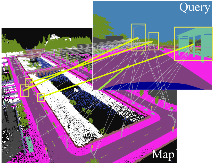
Figure 1: Global localization is solved by estimating true correspondences between instances in a query and those in the prior map. The proposed graph-theoretic framework is potentially applicable to various query and map modalities.

With such a prospect, we propose a framework of single-shot global localization, formulating it as instance correspondence matching between the query and the prior map and finding a pose in the map that best explains the correspondences. For the correspondence matching, we employ a graph-theoretic method that reduces the problem to the maximum clique problem (MCP). Specifically, we construct a graph called a consistency graph that represents local consistency between correspondence candidates, and find the most likely set of correspondences via MCP on the consistency graph, similarly to [6] etc. The motivation behind the formulation is to abstract the problem to a general graph problem so that it is not constrained on a specific modality of the query and the map. The proposed method can potentially be applied to cross-modal global localization problems as long as a proper consistency criteria can be defined.

In the present work, we implement the framework using 3D semantic point cloud maps as a prior map and a semantic segmentation image as a query for correspondence matching. The consistency of the correspondences are evaluated based on the closeness in appearance from the pose calculated by a correspondence pair. Thanks to the graph-theoretic framework, global localization is realized with a combination of simple consistency criteria that does not require additional data for training. The method thus exploits only a 3D semantic map and a semantic segmentation query, in contrast to recent existing methods [5, 7] that depend on data-driven descriptors for correspondence matching. Our method can, therefore, be easily applied to various environments.

II Related Work

II-A Global localization

There have been various approaches with different techniques and sensor modalities.

Iterative methods Traditionally, global localization has been solved in iterative algorithm such as Monte Carlo localization (MCL) [1] where the belief on the robot’s pose gradually converges by incorporating a temporal sequence of observations as the robot moves. This approach inherently requires motion of the robot, which limits the use case of the methods. In the present work, we opt for a single-shot global localization approach.

Global descriptor matching Global descriptor-based methods learn a discriminative descriptor per scene from the sensor observations. The pose is then estimated by matching the descriptor for the observation and pre-computed set of descriptors associated with a pose. This line of work includes Visual Place Recognition (VPR) [2, 3], geometry-based methods [8, 9], and hybrid methods [10, 11].

Local geometry matching In visual global localization, another popular approach is matching local visual features such as SIFT [12] and SURF [13] between a query image and a pre-computed map and optimizing the pose based on the feature correspondences [4, 14]. In 3D LiDAR-based geometry matching, local point descriptors such as [15] and point segments [5, 7] are often used.

Semantics-based localization Following the recent progress of semantic segmentation based on DNNs, global localization methods based on visual semantic information have also been actively studied. Results of semantic segmentation are reported to be more robust to appearance changes than low-level visual information such as feature points [16]. Semantic information has been, therefore, exploited to realize localization methods that are robust to appearance changes over time and viewpoint changes [17].

DNN-based pose regression DNNs are also exploited to directly estimate a sensor pose. Kendal et al. [18] first proposed to regress a 6 DOF pose directly from an image. Feng et al. [19] jointly trained the descriptors for 2D images and 3D points to match data in those different modalities. This approach, again, is specialized to the data on which the network is trained and hard to apply to various scenes.

Problems in existing work and novelties of our work Regardless of the approaches, most of the conventional methods use a query and a map in the same modality. On the other hand, the proposed method does not strictly assume the same modality. Our method, therefore, is potentially applicable to various types of maps such as point cloud maps and HD vector maps.

Although some recent works use DNNs to learn a strong global/local descriptor [2, 5], or to embed data from different modalities in a common feature space [19], such methods require a huge amount of training data. Moreover, pose regression using DNN is specialized to the data on which the model is trained, and difficult to apply to various scenes.

Our primary purpose is to develop a novel unified framework for global localization applicable to cross-modal settings. The pose is efficiently estimated using the graph-theoretic correspondence matching and simple criteria of appearance similarity. We show the effectiveness in an implementation using a semantic point cloud map and a semantic segmentation image.

II-B Correspondence matching

Correspondence matching is a crucial task for some of the aforementioned methods. Random sample consensus (RANSAC) is traditionally used to extract correspondences out of candidates including outliers [14, 4]. Although it shows a high robustness against false positive matches, the number of iterations to achieve a reasonable result increases exponentially as a noise ratio increases due to its stochasticity, and thus is not applicable to cases of high outlier rates.

Graph-theoretic correspondence extraction has been recently shown effective under a high outlier rate where RANSAC fails to extract correspondences [6]. Bailey et al. [20] was one of the earliest to frame data association as MCP. The point association via MCP has been applied to global registration of point cloud [6] [21]. Koide et al. [22] proposed an automatic localization of fiducial tags on a 3D prior map using MCP-based data association.

To the best of our knowledge, this work is the first attempt to employ MCP-based correspondence matching for global localization. The proposed method leverages the graph-theoretic approach to efficiently find the most likely instance correspondences and carries out stable global localization.

III Global Localization via Correspondence Matching by MCP

The general algorithm of the proposed framework of global localization is shown in Algorithm 1. The core of the framework is to estimate the correspondences between the query instances and the map instances to calculate the pose that matches the correspondences the best. To this end, we employ graph-theoretic correspondence matching.

First, we generate candidates for correspondences between a query instance and a map instance. Here, we treat all possible pairs of an instance in the query and one in the map as valid candidates for correspondences.

Once the correspondence candidates are generated, we build a consistency graph, a node of which represents a candidate of correspondence between an instance in the query and one in the map, and an edge indicates consistency between two candidates represented by the nodes connected by the edge. All possible pairs of two correspondence candidates are evaluated based on certain consistency criteria, and if two candidates are evaluated as consistent, an edge is added between the nodes.

The correspondences are then estimated by solving MCP on the consistency graph, and the robot pose is calculated using the extracted correspondences so that it best satisfies the observations of the instances.

Algorithm 1 Global localization via graph-theoretic correspondence matching

0:  Map instance set $\mathcal{M}=\left\{m_{i}\right\}^{N_{m}}_{i=1}$, query instance set $\mathcal{Q}=\left\{q_{j}\right\}^{N_{q}}_{j=1}$

0:  3-DOF robot pose $\left(x,y,\theta\right)$

1:  Correspondence candidate set $\mathcal{C}=\mathcal{M}\times\mathcal{Q}$

2:  Vertex set $\mathcal{V}=\mathcal{C}$

3:  Edge set $\mathcal{E}=\mathbb{0}$

4:  for every combination of $c_{i},c_{j}\in\mathcal{C}$ do

5:     if is_consistent$\left(c_{i},c_{j}\right)$ then

6:        $\mathcal{E}\leftarrow\mathcal{E}\cup\left\{e_{ij},e_{ji}\right\}$

7:     end if

8:  end for

9:  $\mathcal{C}^{\ast}\leftarrow$max_clique$\left(\mathcal{V},\mathcal{E}\right)$

10:  $\left(x,y,\theta\right)\leftarrow$calculate_pose$\left(\mathcal{C}^{\ast}\right)$

11:  return  $\left(x,y,\theta\right)$

IV Implementation on 3D Semantic Map and a Semantic Segmentation Image

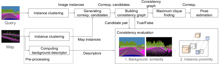
Figure 2: Overview of the proposed framework. As pre-processing, the map instances are clustered, and the grid histogram descriptors (see 4) are computed, and stored as a database. Given a query image, instances are clustered and correspondence candidates are generated as all possible combinations of a query and a map instances. For every pair of the candidates, a pose is calculated (IV-B1) and the consistency is evaluated based on two criteria 1) background similarity, and 2) instance proximity to construct a consistency graph (IV-B2). The most likely set of correspondences is yielded by solving MCP on the consistency graph, and the pose is calculated based on it (IV-C).

Here, we implement the proposed framework using 3D labeled point cloud map as a prior map, and a semantic segmentation image as a query. We consider estimation of a 3 DOF pose $(x,y,\theta)$ of the ground robot. We assume a robot with a camera facing forward and that its transformation relative to the robot’s base is known, and a semantic segmentation image for an image taken by the camera is available. The overview of the workflow is shown in Fig. 2.

IV-A Clustering the map and the query instances

The instances of the 3D map are clustered and individually saved before the localization process. Here, the following four object classes are used for correspondence matching: pole, traffic sign, traffic light, static.

The map points are simply clustered based on their object class and spacial closeness. For the query image, the instances are clustered based on the connectivity. This may wrongly extract multiple instances overlapping in the image as one. We, however, treat such “connected” instances as an individual instance, expecting that they will be rejected in the subsequent process while there still remain sufficient correspondences for pose estimation. Candidates of instance correspondences are all patterns of pairs of instances with the same object class between the map and the image.

IV-B Consistency evaluation

For every combination of two correspondence candidates, a pose is calculated so that it matches the size and the location of image instances and reprojection of the corresponding map instances. The consistency of the pair is then evaluated based on the similarity of the appearance between the query and the map reprojection from the calculated pose.

IV-B1 Pose calculation using a correspondence pair

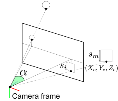
((a)) Angle defined by image instances

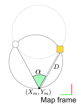
((b)) Circle $C$ defined by inscribed angle $\alpha$

Figure 3: The candidate regions of the robot pose based on the inscribed angle and the size of the instance. (b) The translation of the camera $(X_{m},Y_{m})$ in the map frame is determined as a point on $C$ where the distance to an object is $D=\sqrt{X_{c}^{2}+Z_{c}^{2}}$.

Given two image instances, an angle $\alpha$ formed by two vectors to each image instance from the origin of the camera frame is determined. The region of the pose is then constrained to a circle $C$ that has an inscribed angle $\alpha$ as shown in Fig. 3. Since there are two such circles, we determine $C$ based on the positional relationship of the instances.

To determine the pose, we use the scale information of one of the correspondences. The relationship of the size in the 3D space $s_{m}$ and that of its projection $s_{i}$ is written as:

$$s_{i}=\frac{f\cdot s_{m}}{Z_{c}},$$ (1)

where $f$ denotes the focal length of the camera and $Z_{c}$ denotes the $Z$ coordinate of the instance in the camera frame. Since the sizes of both image instance and the map instance in a correspondence are known, $Z_{c}$ can be estimated as:

$$Z_{c}=\frac{f\cdot s_{m}}{s_{i}}.$$ (2)

The set of points that satisfy eq. (2) also forms a circle with a radius $D=\sqrt{X_{c}^{2}+Z_{c}^{2}}$. The camera pose can, therefore, be calculated as an intersection of circle $C$ and a circle that centers at the location of the map instance and has radius $D$. In this way, at most two intersections are yielded. In such a case, we calculate the expected size of the projection of another map instance using eq. (1) from the two poses, and compare them with the size of the corresponding image instance. The pose that provides a smaller error of the size is selected as the solution.

IV-B2 Consistency criteria

The consistency is evaluated based on two criteria, background similarity and instance proximity. The latter is relevant to the spacial consistency, which is often employed in MCP-based correspondence matching such as [6] and [22]. In our problem, however, this criterion is not sufficient because there may be many wrong correspondences that happen to satisfy it. The background similarity criterion is, therefore, employed before the instance proximity to filter out unlikely correspondences based on the appearance similarity. Using the two criteria, we effectively evaluate consistency of the correspondences.

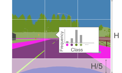
((a)) Grid histogram

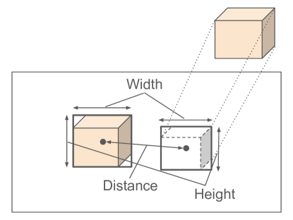
((b)) Instance proximity

Figure 4: Consistency criteria. (a) The grid histogram descriptor is a normalized vector of the local histograms of object classes. (b) The instance proximity evaluates a spacial relationship between the bounding boxes around the image instance and the projection of the map instance.

Background similarity The purpose of the background similarity criterion is not to strictly detect images similar to the query, but to quickly filter out obvious outliers. To this end, we employ a simple histogram descriptor.

Fig. 4(a) shows an overview. First, the bottom of the image is cut off as this part does not convey much information. The remaining part of the image is divided into grids with a fixed size. For each grid, a histogram of the object classes is generated and L2-normalized. We chose nine background object classes: building, fence, road line, road, sidewalk, vegetation, wall, bridge, terrain. The normalized histograms from the grids are concatenated into ($h\times w\times 9$)-dimensional vector, where $h$ and $w$ denotes the number of grid in the vertical and the horizontal axis, respectively. The vector is then L2-normalized again to form a descriptor. Similarity of two descriptors are given as a dot product, or equivalently a cosine similarity with a value range of $[0,1]$.

For fast evaluation, we pre-compute the descriptors for the map by projecting the 3D map from the poses uniformly sampled in the map.

Instance proximity The instance proximity is evaluated by the distance and the size differences of bounding boxes around the projected map instance and the image instance (see Fig. 4(b)). The distance between them are defined as the Euclidean distance between the centroids of the bounding boxes. The size differences are calculated with height and width lengths of the bounding boxes. If the distance, the height and the width difference are all less than a threshold for both of the correspondences in the given pair, the pair of correspondence candidates is considered consistent.

Here, we set the threshold adaptively to the $Z$ coordinate value $Z_{c}$ of each map instance in the camera frame. We empirically define the distance threshold $\theta_{d}$ and the size threshold $\theta_{s}$ as follows:

$$\theta_{d} =\min\left(m_{d},\max\left(m_{min},dm_{d}/Z_{c}\right)\right)$$ (3)

$$\theta_{s} =\min\left(m_{s},\max\left(m_{min},dm_{s}/Z_{c}\right)\right),$$

where $m_{d}$ and $m_{s}$ denote the maximum possible threshold of the instance distance and the size in pixel, respectively. The idea behind these definitions is to set the thresholds of objects at $d$ [m] from the sensor to $m_{d}$ [px] and $m_{s}$ [px], and decrease it as $Z_{c}$ becomes larger. The thresholds are clipped with the minimum value of $m_{min}$ [px] and the maximum value of $m_{d}$ and $m_{s}$. Here, we set $d$ to 8 and $m_{min}$ to 5.

IV-C Pose estimation

A consistency graph is constructed based on the aforementioned consistency criteria, and the most likely set of correspondences are yielded by solving as described in IV. The final pose is then calculated by minimizing the reprojection error of representation points of the correspondences. A representation point of an image instance is a point that has the largest y value in the image coordinate, and that of a map instance is the point with the smallest z value in the map coordinate, representing their bottom point. Although this way does not provide exact matching of the parts of the instances, it does not affect much the calculation of the camera pose. An initial pose is given as an average of poses calculated by the correspondences in the clique during the phase of building the consistency graph (see IV-B1). The Levenberg-Marquardt algorithm [23, 24] with Huber kernel [25] is applied to the pose optimization.

IV-D Pose verification via correspondence check

Ideally, the maximum clique of the consistency graph represents a set of correct correspondences. In practice, however, we found that it is often not the case due to rejection of the correct correspondences mainly caused by error in pose calculation, while evaluating wrong ones as consistent.

To mitigate the problem, we introduce a verification step. After constructing the consistency graph, we calculate multiple correspondence set by iteratively applying MCP solver, calculating a pose with each set, and removing edges between the vertices corresponding to the members of the found maximum clique. To verify each correspondence set, we count the number of image instances that have a map instance projected close to it from the calculated pose based on the proximity criterion. The correspondence set with the maximum count is treated as the result. Top N results are yielded by taking results with five largest counts.

V Experiments

V-A Experimental setup

The experiments were conducted on a laptop with an Intel Core i7-10750H (12 threads) and 16 GB of RAM.

We used simulated point cloud maps of Town01 to 05 from CARLA simulator [26] for evaluation. The description of the environments is shown in Table 1. We created point cloud maps using the scripts shared by the authors of [27]. For each map, descriptors are pre-computed from the poses uniformly sampled with a stride of 2 m in the x and the y axes of the map frame and $30^{\circ}$ in the yaw angle.

The samples of query were generated from the spawn points of vehicles defined in CARLA. A camera was mounted on the simulated vehicle at the height of approx. 1.5 m from the robot’s base. Since the proposed method estimates a 3 DOF pose and assumes fixed height of the camera, we choose the poses with the height between 1.46 m and 1.90 m as the samples. We use ground truth semantic segmentation images generated by CARLA.

TABLE I: Descriptions of the CARLA Towns

Town	Summary
01	A basic town layout consisting of ”T junctions”.
02	Similar to Town01, but smaller.
03	The most complex town, with a 5-lane junction, a roundabout, unevenness, a tunnel, and more.
04	An infinite loop with a highway and a small town.
05	Squared-grid town with cross junctions and a bridge. It has multiple lanes per direction.

The thresholds of the background similarity (BS), the instance distance and the instance size in the instance proximity (IP) are empirically set to 0.9, 110, 50, respectively.

V-B Baselines

As baselines, we use brute-force descriptor search (BF) and RANSAC-based correspondence matching. The former searches for the pre-computed descriptor that has the highest similarity score with the query and returns the discretized pose that the descriptor is associated with. In the latter, RANSAC is used for correspondence finding instead of the proposed graph-theoretic approach. For a randomly sampled pair of correspondences, a pose is calculated as described in IV-B1 and the number of the correspondences consistent with the pose is counted. We use the same background similarity threshold as the proposed method to reject the pair, and the instance proximity threshold to find the correspondences. The number of iteration is set to 50000.

V-C Evaluation conditions

We evaluate the localization performance using three conditions: $\pm$5, $\pm$10, and front drift. For all of the conditions, the threshold of yaw error is $\pm 30^{\circ}$. $\pm$5 denotes the case where the lateral and longitudinal errors are within $\pm 5$ m. Likewise, $\pm$ 10 means within $\pm$ 10 m of lateral and longitudinal errors. Front drift denotes the case where the error in the x axis of the robot’s frame is within $\pm 200$ m and $\pm 5$ m in the y axis. This is typically the case when the estimated pose is on the same road as the ground truth and facing the same direction, but is drifted in the longitudinal direction in the robot frame.

V-D Localization results

TABLE II: Results of global localization

Town		01	02	03	04	05
Samples		254	101	197	259	234
$\pm$5	T1	133	60	63	36	76
		(52.4%)	(59.4%)	(32.0%)	(13.7%)	(32.5%)
	T3	157	68	73	45	93
		(61.8%)	(67.3%)	(37.1%)	(17.4%)	(39.7%)
	T5	167	71	79	48	98
		(65.7%)	(70.3%)	(40.1%)	(18.5%)	(41.9%)
$\pm$10	T1	142	65	72	49	81
		(55.9%)	(64.4%)	(36.5%)	(18.9%)	(34.6%)
	T3	170	74	85	62	100
		(66.9%)	(73.3%)	(43.1%)	(23.9%)	(42.7%)
	T5	183	77	94	67	106
		(72.0%)	(76.2%)	(47.7%)	(25.9%)	(45.3%)
FD	T1	175	75	95	53	87
		(68.9%)	(74.3%)	(48.2%)	(20.5%)	(37.2%)
	T3	196	81	104	76	110
		(77.2%)	(80.2%)	(52.8%)	(27.8%)	(47.0%)
	T5	207	86	114	82	123
		(81.5%)	(85.1%)	(57.9%)	(30.1%)	(52.6%)

• * T1, T3, and T5 denote Top 1, Top 3, and Top 5, respectively. FD denotes Front drift. Green: $>70$ %, Red: $<30$ %

Table II shows the results of global localization. The values indicate the number of samples that resulted in fulfilling the evaluation conditions in Top 1, Top 3, and Top 5 results calculated as described in IV-D. In Town01 and 02, Top 5 estimation for approximately 65 to 70 % of the samples fulfilled $\pm$5, and more than 80 % of them fulfilled front drift. In Town 03 and 05, Top 5 results of approximately 40 % samples fulfilled $\pm$5. The result of Town04 was significantly worse than the other maps, with 18.5 % of $\pm$5 and 30.1 % of front drift in Top 5 results, respectively. We discuss the cause of the low performance in V-G.

V-E Comparison with the baselines

Table III shows the comparative results with the baselines. The values are the number of Top 1 results of $\pm$5 and $\pm$10. The proposed method surpassed the baseline methods in all conditions but $\pm$10 of BF in Town05. It is worth noting that the brute-force search did not result in accurate pose estimation in most of the environments. Nevertheless, combined with our framework, it resulted in better performance. RANSAC was also resulted in worse results than the proposed method. This is an expected result as most of the correspondence candidates are outliers in the tasks, and RANSAC struggles with finding a consistent pair via random sampling. In contrast, the proposed method efficiently found the correspondences leveraging the graph-theoretic approach.

TABLE III: Comparison with the baselines

	Town no.	01	02	03	04	05
	Samples	254	101	197	259	234
BF	$\pm$5	99	35	49	32	70
	$\pm$10	107	34	62	47	98
RANSAC	$\pm$5	17	7	5	2	6
	$\pm$10	22	10	17	11	12
Proposed	$\pm$5	133	60	63	36	76
	$\pm$10	142	65	72	49	81

V-F Ablation studies on the consistency criteria

TABLE IV: Ablation on the consistency criteria

Town no.	01	02	03	04	05
Samples	254	101	197	259	234
BS(0.9)	40	18	6	1	8
IP/IP+BS(0.5)	18*	8	4	11	15
IP+BS(0.9)	133	60	63	36	76

• Only IP

Table IV shows the results of an ablation study on the consistency criteria to examine their contribution. To test IP for Town02 to 05, we loosened BS threshold to 0.5 (denoted as IP+BS(0.5)) instead of using only IP, because we found disabling BS significantly slowed down the computation speed due to increased number of transformation of map instances in IP computation.

As a result, the performance was significantly worse in BS and IP (Town01) / IP+BS(0.5) (02-05). The combination of those simple consistency criteria resulted the best to effectively find the correspondences and calculate the pose.

V-G Discussion

We saw promising results of the proposed framework especially in Town01 and 02. Notably, the proposed method requires only the semantic 3D map and semantic segmentation query. Although the building blocks for consistency evaluation are simple, our system provided reasonable results. We suppose this is thanks to the graph-theoretic correspondence matching approach which is capable of effectively extracting correspondences under high outlier rate.

Limitations Despite the powerful graph-theoretic approach, there were also many failure cases. They mainly stem from the error in the pose estimation using a pair of correspondences. The current pose calculation is sensitive to noise in instance clustering because it exploits the relationship of the scales of instances to estimate the distance from the robot pose to the map instances, and assumes that both the image instance and the map instance are complete. In reality, however, the assumption often does not hold. This problem will also affect real-world application because, in practice, the query semantic segmentation will be provided by an estimator based on DNNs etc., which inevitably has estimation noise. To deal with it, we should introduce pose calculation that is more robust to such noise.

The causes of the low accuracy for Town04 are twofold. First, the number of image instances are fewer than other Towns. Due to the unstable pose calculation, a few image instances in an image are generally rejected in MCP, and it is thus more possible to result in no correct correspondences detected when an image has few instances. Second, the mountains and terrains seen far away in the query were not mapped due to the limited range of the point cloud map, and the descriptors of the query and the map had a large difference in many samples. This effect was especially significant in Town04 consisting of open highway scenes with mountains. Although the simple descriptor provided reasonable results in tandem with the proposed framework, we should reconsider its design to mitigate such a problem.

VI Conclusion

We proposed a framework for global localization based on graph-theoretic matching of instance correspondences between a query and a prior map. We implemented the framework on semantically labeled point cloud maps and semantic segmentation images as queries. Leveraging the efficient graph-theoretic correspondence matching with the simple consistency criteria, we presented promising preliminary results on the global localization task in simulated urban environments. This research direction will lead to localization ability of robots with more flexibility of of the map and sensor modalities.

References

- [1] Frank Dellaert, Wolfram Burgard, Dieter Fox and Sebastian Thrun “Using the CONDENSATION algorithm for robust, vision-based mobile robot localization” In IEEE/CVF Conference on Computer Vision and Pattern Recognition IEEE, 1999, pp. 588–594 DOI: 10.1109/CVPR.1999.784976
- [2] Relja Arandjelovic, Petr Gronat, Akihiko Torii, Tomas Pajdla and Josef Sivic “NetVLAD: CNN Architecture for Weakly Supervised Place Recognition” In IEEE Transactions on Pattern Analysis and Machine Intelligence 40.6, 2018, pp. 1437–1451 DOI: 10.1109/TPAMI.2017.2711011
- [3] Ahmad Khaliq, Michael Milford and Sourav Garg “MultiRes-NetVLAD: Augmenting Place Recognition Training with Low-Resolution Imagery” In IEEE Robotics and Automation Letters 7.2 Institute of ElectricalElectronics Engineers Inc., 2022, pp. 3882–3889 DOI: 10.1109/LRA.2022.3147257
- [4] Marcel Geppert, Peidong Liu, Zhaopeng Cui, Marc Pollefeys and Torsten Sattler “Efficient 2D-3D matching for multi-camera visual localization” In IEEE International Conference on Robotics and Automation, 2019, pp. 5972–5978 DOI: 10.1109/ICRA.2019.8794280
- [5] Renaud Dubé, Andrei Cramariuc, Daniel Dugas, Hannes Sommer, Marcin Dymczyk, Juan Nieto, Roland Siegwart and Cesar Cadena “SegMap: Segment-based mapping and localization using data-driven descriptors” In International Journal of Robotics Research 39.2-3, 2020, pp. 339–355 DOI: 10.1177/0278364919863090
- [6] Heng Yang, Jingnan Shi and Luca Carlone “TEASER: Fast and Certifiable Point Cloud Registration” In IEEE Transactions on Robotics 37.2, 2021, pp. 314–333 DOI: 10.1109/TRO.2020.3033695
- [7] Andrei Cramariuc, Florian Tschopp, Nikhilesh Alatur, Stefan Benz, Tillmann Falck, Marius Bruhlmeier, Benjamin Hahn, Juan Nieto and Roland Siegwart “SemSegMap – 3D Segment-based Semantic Localization” In IEEE/RSJ International Conference on Intelligent Robots and Systems IEEE, 2021, pp. 1183–1190 DOI: 10.1109/IROS51168.2021.9636156
- [8] Huan Yin, Li Tang, Xiaqing Ding, Yue Wang and Rong Xiong “LocNet: Global Localization in 3D Point Clouds for Mobile Vehicles” In IEEE Intelligent Vehicles Symposium IEEE, 2018, pp. 728–733 DOI: 10.1109/IVS.2018.8500682
- [9] Konrad P. Cop, Paulo V K Borges and Renaud Dube “Delight: An Efficient Descriptor for Global Localisation Using LiDAR Intensities” In IEEE International Conference on Robotics and Automation IEEE, 2018, pp. 3653–3660 DOI: 10.1109/ICRA.2018.8460940
- [10] Johannes L. Schonberger, Marc Pollefeys, Andreas Geiger and Torsten Sattler “Semantic Visual Localization” In IEEE/CVF Conference on Computer Vision and Pattern Recognition IEEE, 2018, pp. 6896–6906 DOI: 10.1109/CVPR.2018.00721
- [11] Sebastian Ratz, Marcin Dymczyk, Roland Siegwart and Renaud Dube “OneShot Global Localization: Instant LiDAR-Visual Pose Estimation” In IEEE International Conference on Robotics and Automation, 2020, pp. 5415–5421 DOI: 10.1109/ICRA40945.2020.9197458
- [12] David G Lowe “Distinctive Image Features from Scale-Invariant Keypoints” In International Journal of Computer Vision 60.2, 2004, pp. 91–110 DOI: 10.1023/B:VISI.0000029664.99615.94
- [13] Herbert Bay, Tinne Tuytelaars and Luc Van Gool “SURF: Speeded Up Robust Features” In European Conference on Computer Vision, 2006, pp. 404–417 DOI: 10.1007/11744023˙32
- [14] Stephen Se, David G. Lowe and James J. Little “Vision-based global localization and mapping for mobile robots” In IEEE Transactions on Robotics 21.3, 2005, pp. 364–375 DOI: 10.1109/TRO.2004.839228
- [15] Radu Bogdan Rusu, Nico Blodow and Michael Beetz “Fast Point Feature Histograms (FPFH) for 3D registration” In IEEE International Conference on Robotics and Automation IEEE, 2009, pp. 3212–3217 DOI: 10.1109/ROBOT.2009.5152473
- [16] Semih Orhan, Jose J. Guerrero and Yalin Bastanlar “Semantic Pose Verification for Outdoor Visual Localization with Self-supervised Contrastive Learning” In IEEE/CVF Conference on Computer Vision and Pattern Recognition Workshops IEEE, 2022, pp. 3989–3998 arXiv:2203.16945
- [17] Xiyue Guo, Junjie Hu, Junfeng Chen, Fuqin Deng and Tin Lun Lam “Semantic Histogram Based Graph Matching for Real-Time Multi-Robot Global Localization in Large Scale Environment” In IEEE Robotics and Automation Letters 6.4 IEEE, 2021, pp. 8349–8356 DOI: 10.1109/LRA.2021.3058935
- [18] Alex Kendall, Matthew Grimes and Roberto Cipolla “PoseNet: A Convolutional Network for Real-Time 6-DOF Camera Relocalization” In IEEE International Conference on Computer Vision IEEE, 2015, pp. 2938–2946 DOI: 10.1109/ICCV.2015.336
- [19] Mengdan Feng, Sixing Hu, Marcelo H. Ang and Gim Hee Lee “2D3D-Matchnet: Learning To Match Keypoints Across 2D Image And 3D Point Cloud” In IEEE International Conference on Robotics and Automation 2019-May IEEE, 2019, pp. 4790–4796 DOI: 10.1109/ICRA.2019.8794415
- [20] T. Bailey, E.M. Nebot, J.K. Rosenblatt and H.F. Durrant-Whyte “Data association for mobile robot navigation: a graph theoretic approach” In IEEE International Conference on Robotics and Automation IEEE, 2000, pp. 2512–2517 DOI: 10.1109/ROBOT.2000.846406
- [21] Jingnan Shi, Heng Yang and Luca Carlone “ROBIN: a Graph-Theoretic Approach to Reject Outliers in Robust Estimation using Invariants” In IEEE International Conference on Robotics and Automation IEEE, 2021, pp. 13820–13827 DOI: 10.1109/ICRA48506.2021.9562007
- [22] Kenji Koide, Shuji Oishi, Masashi Yokozuka and Atsuhiko Banno “Scalable Fiducial Tag Localization on a 3D Prior Map via Graph-Theoretic Global Tag-Map Registration” In IEEE/RSJ International Conference on Intelligent Robots and Systems IEEE, 2022 arXiv:2207.11942
- [23] Kenneth Levenberg “A method for the solution of certain non-linear problems in least squares” In Quarterly of Applied Mathematics 2.2 Brown University, 1944, pp. 164–168 DOI: 10.1090/qam/10666
- [24] Donald W Marquardt “An Algorithm for Least-Squares Estimation of Nonlinear Parameters” In Journal of the Society for Industrial and Applied Mathematics 11.2, 1963, pp. 431–441 DOI: 10.1137/0111030
- [25] Peter J. Huber “Robust Estimation of a Location Parameter” In The Annals of Mathematical Statistics 35.1, 1964, pp. 73–101 DOI: 10.1214/aoms/1177703732
- [26] Alexey Dosovitskiy, German Ros, Felipe Codevilla, Antonio Lopez and Vladlen Koltun “CARLA: An Open Urban Driving Simulator” In Conference on Robot Learning PMLR, 2017, pp. 1–16 arXiv:1711.03938
- [27] Jean Emmanuel Deschaud, David Duque, Jean Pierre Richa, Santiago Velasco-Forero, Beatriz Marcotegui and François Goulette “Paris-carla-3d: A real and synthetic outdoor point cloud dataset for challenging tasks in 3d mapping” In Remote Sensing 13.22, 2021, pp. 1–24 DOI: 10.3390/rs13224713