On $G_{2}$ manifolds with cohomogeneity two symmetry

Abstract.

We consider $\operatorname{G_{2}}2$ manifolds with a cohomogeneity two $\operatorname{\mathbb{T}}^{2}\times\operatorname{SU}(2)$ symmetry group. We give a local characterization of these manifolds and we describe the geometry, including regularity and singularity analysis, of cohomogeneity one calibrated submanifolds in them. We apply these results to the manifolds recently constructed by Foscolo–Haskins–Nördstrom and to the Bryant–Salamon manifold of topology ${\ooalign{$S$\cr$/$\cr}}(S^{3})$. In particular, we describe new large families of complete $\operatorname{\mathbb{T}}^{2}$-invariant associative submanifolds in them.

1. Introduction

In a Riemannian manifold, parallel transport with respect to the Levi-Civita connection is used to define its Riemannian holonomy group. The groups that can appear as the holonomy of a simply-connected, nonsymmetric and irreducible Riemannian manifold were classified by Berger in [8]. All but two elements of Berger’s list come in a countable family depending on the dimension of the manifold. The exceptional cases are $\operatorname{G_{2}}2$ and $\operatorname{Spin}(7)$, which are only related to Riemannian manifolds of dimension $7$ and $8$, respectively. Manifolds with holonomy $\operatorname{G_{2}}2$, called $\operatorname{G_{2}}2$ manifolds, are Ricci-flat [35, Lemma 11.8] and admit two natural classes of volume minimizing submanifolds: the associative $3$-folds and the coassociative $4$-folds, which are in particular calibrated submanifolds [19].

Bryant and Salamon constructed the first complete $\operatorname{G_{2}}2$ manifolds with full holonomy more than 30 years ago in [11]. Since then, much effort has been spent to construct new examples of such manifolds (e.g. [17, 15, 32, 34, 16, 9, 10]) and study their calibrated submanifolds (e.g. [22, 23, 24, 26]). Even though we now have a lot of examples of non-compact manifolds with Riemannian holonomy $\operatorname{G_{2}}2$ (mainly because of the seminal work by Foscolo–Haskins–Nordström and Foscolo [16, 15, 17]), only a few non-trivial associative and coassociative submanifolds were constructed in them.

One of the most successful techniques used to construct non-compact $\operatorname{G_{2}}2$ manifolds is symmetry reduction, which means that the manifold admits a structure-preserving, hence isometric, Lie group action. Particular attention has been given to the cohomogeneity one and to the abelian case. Indeed, under the former assumption, the system of PDEs characterising the $\operatorname{G_{2}}2$ holonomy condition becomes a system of ODEs and many examples were constructed in this way (cfr. [17, 9, 10, 11]). Under the latter assumption, the problem reduces to finding a torus bundle with curvature constraints over a lower dimensional manifold with some special structure (cfr. [32, 34, 12, 3]). This technique often relies on the multi-moment maps introduced by Madsen and Swann in [32, 33], which are generalisations of classical moment maps in symplectic geometry. The authors are not aware of any previous attempt towards a better understanding of the intermediate case, i.e. non abelian groups of higher cohomogeneity.

For what concerns calibrated geometry, associative and coassociative submanifolds are in general hard to construct. Indeed, they are solutions of a system of non-linear PDEs. However, in the setting above, we have special calibrated submanifolds which are easier to study: the ones that are invariant under a cohomogeneity one symmetry. Indeed, the invariance turns the system of PDEs into a system of ODEs on the set of orbits. This idea was successful on the flat $\mathbb{R}^{7}$ with the standard $\operatorname{G_{2}}2$-structure [29, 30, 19] and on the Bryant–Salamon manifold of topology $\Lambda^{2}_{-}(S^{4})$ and $\Lambda^{2}_{-}(\mathbb{C}\mathbb{P}^{2})$ for coassociative submanifolds [26, 23]. Note that in both cases the $\operatorname{G_{2}}2$-structure of the manifold is explicit, and so is the system of ODEs.

By the local existence and uniqueness theorem for associatives and coassociatives [19] (or simply by ODE theory), the calibrated submanifolds constructed in this way do not intersect and are smooth in the principal set of the action. However, this may not be the case in the singular set. Indeed, there are examples of singular and/or intersecting cohomogeneity one calibrated submanifolds, such as the $\operatorname{\mathbb{T}}^{2}$-invariant special Lagrangian cone in $\mathbb{C}^{3}$, called Harvey–Lawson cone, which induces a $\operatorname{\mathbb{T}}^{2}$-invariant associative cone in $\mathbb{R}^{7}$ (see [30, 23, 29, 19] for further examples).

If we consider $\operatorname{\mathbb{T}}^{3}$-invariant coassociatives, Madsen and Swann observed in [34] that the multi-moment maps relative to the $\operatorname{\mathbb{T}}^{3}$-action are first integrals of the coassociative system, which completely determine the desired submanifolds for dimensional reasons. Afterwards, the connection between non-abelian multi-moment maps and calibrated submanifolds was investigated by Karigiannis–Lotay [23] and the second named author [39] on the $\operatorname{G_{2}}2$ Bryant–Salamon manifolds and on the $\operatorname{Spin}(7)$ Bryant–Salamon manifold, respectively.

Another method used on the Bryant–Salamon spaces $\Lambda^{2}_{-}(S^{4})$ and $\Lambda^{2}_{-}(\mathbb{C}\mathbb{P}^{2})$ was to look for calibrated submanifolds which are (possibly twisted) vector subbundles over suitable submanifolds of the zero section [24, 22]. Neither the cohomogeneity one nor the vector subbundle technique were adapted to the Bryant–Salamon manifolds of topology ${\ooalign{$S$\cr$/$\cr}}(S^{3})$, where the only known calibrated submanifolds were the zero section, which is associative, and the fibres over a given point, which are coassociatives. To the best knowledge of the authors, there are no other non-trivial examples of calibrated submanifolds in non-flat and non-compact $\operatorname{G_{2}}2$ manifolds.

Note that even though we lose the calibrated condition, hence the volume minimizing property, the notion of associative and coassociative submanifolds makes sense and has been studied for weaker notions of $\operatorname{G_{2}}2$ manifolds, such as closed, co-closed or nearly-parallel $\operatorname{G_{2}}2$ manifolds (cfr. [4, 5, 31, 25, 6] and references therein).

An additional important aspect of manifolds with special holonomy, which we only tangentially touch upon in this paper, is finding and making use of calibrated fibrations. These objects are not only interesting from a mathematical perspective but should also play a crucial role in mathematical physics (cfr. the SYZ conjecture [38] and its generalizations [18]). For this reason, calibrated fibrations in manifolds of special holonomy have been widely studied by both communities (e.g. [39, 23, 13, 27, 28, 1, 7]).

1.1. Main results

In this work, we investigate $\operatorname{G_{2}}2$ manifolds endowed with a structure-preserving, cohomogeneity two action of the non-abelian Lie group $\operatorname{\mathbb{T}}^{2}\times\operatorname{SU}(2)$, and the relative calibrated geometry. Note that there are a lot of $\operatorname{G_{2}}2$ manifolds with such a group action. For instance, the large class of examples constructed by Foscolo–Haskins–Norsdström in [17] (FHN manifolds for brevity) has the desired symmetry, in fact, they admit a $\operatorname{SU}(2)\times\operatorname{SU}(2)\times\operatorname{U}(1)$ cohomogeneity one and structure-preserving action. Moreover, all simply-connected complete $\operatorname{G_{2}}2$-manifolds with $\operatorname{SU}(2)\times\operatorname{SU}(2)\times\operatorname{U}(1)$-symmetry arise in this way [17, Theorem 7.3]. Special elements of this family are the Bryant–Salamon manifold of topology ${\ooalign{$S$\cr$/$\cr}}(S^{3})$ and the asymptotically locally conical manifolds constructed by Bogoyavlenskaya [9], which were previously predicted by Brandhuber–Gomis–Gubser–Gukov [10]. Apart from these, which have enhanced symmetry, one can find examples with a genuine $\operatorname{\mathbb{T}}^{2}\times\operatorname{SU}(2)$-action of cohomogeneity two in [15, Theorem 4.12], assuming $p_{1}=p_{2}$ and $q_{1}\neq q_{2}$. In the co-closed case, Alonso constructed examples of $\operatorname{G_{2}}2$ manifolds with $\operatorname{SU}(2)\times\operatorname{SU}(2)\times\operatorname{U}(1)$-symmetry [2].

As a first step, we study the stabilizer subgroups that can arise in this setting (Theorem 3.7) and, then, we give a local characterization of such manifolds in the principal set (Theorem 4.8).

Theorem.

Let $(M,\varphi)$ be a $\operatorname{G_{2}}2$ manifold with a $\operatorname{\mathbb{T}}^{2}\times\operatorname{SU}(2)$ cohomogeneity-two action. Then, the action has no exceptional orbits, and, in the principal set, it can be locally reconstructed from two nested systems of ODEs and a suitable two-form, representing the curvature of a $\operatorname{\mathbb{T}}^{2}$-bundle.

Afterwards, we consider $\operatorname{\mathbb{T}}^{2}\times\mathrm{Id}_{\operatorname{SU}(2)}$-invariant associatives, $\operatorname{\mathbb{T}}^{3}\cong\operatorname{\mathbb{T}}^{2}\times S^{1}$-invariant coassociatives and $\mathrm{Id}_{\operatorname{\mathbb{T}}^{2}}\times\operatorname{SU}(2)$-invariant coassociatives. In particular, we give a nice characterization of these objects in the $\operatorname{\mathbb{T}}^{2}\times\operatorname{SU}(2)$-quotient of the principal set (Theorem 5.5, Theorem 6.8 and Theorem 6.15), which is a surface locally parametrized by the $\operatorname{\mathbb{T}}^{2}$-invariant associatives and the $\operatorname{\mathbb{T}}^{3}$-invariant coassociatives (Corollary 6.10). We then, study the regularity of such submanifolds and we deduce the following (cfr. Theorem 5.11, Theorem 6.5 and Theorem 6.20)

Theorem.

Let $(M,\varphi)$ be a $\operatorname{G_{2}}2$ manifold with a $\operatorname{\mathbb{T}}^{2}\times\operatorname{SU}(2)$ cohomogeneity-two action. Then, $\operatorname{\mathbb{T}}^{2}\times\mathrm{Id}_{\operatorname{SU}(2)}$-invariant associatives and $\mathrm{Id}_{\operatorname{\mathbb{T}}^{2}}\times\operatorname{SU}(2)$-invariant coassociatives are smooth, while coassociative submanifolds that are invariant under $\operatorname{\mathbb{T}}^{2}\times S^{1}$ for any $S^{1}$-subgroup of $\operatorname{SU}(2)$ can develop singularities with a tangent cone modelled on the Harvey–Lawson cone times $\mathbb{R}$.

We show that $\operatorname{\mathbb{T}}^{2}$-invariant associatives and $\operatorname{SU}(2)$-invariant coassociatives are smooth everywhere (Theorem 5.11 and Theorem 6.20), while $\operatorname{\mathbb{T}}^{3}$-invariant coassociatives develop singularities, modelled on the Harvey–Lawson cone times a line, on the singular set of the $\operatorname{\mathbb{T}}^{3}$-action with $1$-dimensional stabilizer (Theorem 6.5). Along the way (Corollary 5.10), we prove that under some mild topological conditions the $\operatorname{\mathbb{T}}^{2}$-invariant associatives form an associative fibration, in the same sense as in [23, 39]. Moreover, we outline when our results can be extended to closed or co-closed $\operatorname{G_{2}}2$-manifolds (cfr. Remark 5.13 Remark 6.11 and Remark 6.22).

We conclude applying the aforementioned discussion to the FHN manifolds and to the Bryant–Salamon manifolds of topology ${\ooalign{$S$\cr$/$\cr}}(S^{3})$. In particular, we obtain new large families of complete $\operatorname{\mathbb{T}}^{2}$-invariant associatives (Theorem 7.4 and Theorem 7.5).

Theorem.

Let $(M,\varphi)$ be one of the complete $\operatorname{G_{2}}2$ manifolds with $\operatorname{SU}(2)\times\operatorname{SU}(2)\times\operatorname{U}(1)$-symmetry constructed by Foscolo–Haskins–Nordströrm in [17]. Then, for every $\operatorname{\mathbb{T}}^{2}\cong\mathrm{Id}_{\operatorname{SU}(2)}\times\operatorname{U}(1)\times\operatorname{U}(1)\subset\operatorname{SU}(2)\times\operatorname{SU}(2)\times\operatorname{U}(1)$ (or $\operatorname{\mathbb{T}}^{2}\cong\operatorname{U}(1)\times\mathrm{Id}_{\operatorname{SU}(2)}\times\operatorname{U}(1)\subset\operatorname{SU}(2)\times\operatorname{SU}(2)\times\operatorname{U}(1)$), there are the following families of distinct complete $\operatorname{\mathbb{T}}^{2}$-invariant associatives:

1. a $4$-parameter one with elements of topology $\operatorname{\mathbb{T}}^{2}\times\mathbb{R}$,

2. two distinct $2$-parameter ones whose elemets are of topology $S^{1}\times\mathbb{R}^{2}$,

3. depending on the topology of $M$, one single compact $S^{3}$ or, alternatively, a $2$-parameter family of topological Lens spaces as elements.

Conversely, any complete associative with such a $\operatorname{\mathbb{T}}^{2}$-symmetry belongs to this list.

Furthermore, we extend to ${\ooalign{$S$\cr$/$\cr}}(S^{3})$ the description of (possibily twisted) calibrated subbundles in manifolds of exceptional holonomy started by Karigiannis, Leung and Min-Oo [22, 24] (Proposition 7.6).

1.2. Overview of the paper

Before getting into the main content of this work, we provide, in Section 2, a brief introduction to $\operatorname{G_{2}}2$ geometry and to the relative calibrated submanifolds. Inspired by [39, 23], we also give a definition of calibrated fibrations in which fibres are allowed to be singular and to intersect.

In Section 3, we study the geometry of the $\operatorname{\mathbb{T}}^{2}\times\operatorname{SU}(2)$-action. As a first step, we discuss how to quotient the Lie group, and the relative $\operatorname{\mathbb{T}}^{2}$ or $\operatorname{SU}(2)$ components, so that the action passes to suitable quotients of the $\operatorname{G_{2}}2$ manifold. Even though the group is non-abelian, we are able to classify the stabiliser types and the slice action on the normal bundle (Theorem 3.7). It turns out that there are no exceptional orbits and, using the orbit type theorem, we are able to split our manifold into a stratification given by a principal set $M_{P}$, where the stabilizer is zero-dimensional, and $\mathcal{S}_{i}$ for $i=1,2,3,4$, where the stabilizer is $i$-th dimensional. Finally, we untangle the definition of multi-moment maps [33, Definition 3.9] for this group action, and we establish their invariance and equivariance.

Afterwards, in Section 4, we investigate the local structure of $\operatorname{G_{2}}2$ manifolds with the given cohomogeneity two symmetry. In our setting, we independently consider the $\operatorname{\mathbb{T}}^{2}$ and the $\operatorname{SU}(2)$ factors as follows. Madsen and Swann [33] showed that, under the presence of a $\operatorname{\mathbb{T}}^{2}$-symmetry, Hitchin’s flow preserves the level sets of the $\operatorname{\mathbb{T}}^{2}$ moment map $\nu$, and the quotient $\chi_{t}=\nu(t)/\operatorname{\mathbb{T}}^{2}$ admits a coherent tri-symplectic structure. They also showed how to reconstruct the $\operatorname{G_{2}}2$ manifold with $\operatorname{\mathbb{T}}^{2}$-symmetry from such a four manifold. In our setup, $\chi_{t}$ inherits an additional $\operatorname{SU}(2)$-symmetry. We classify these tri-symplectic structures as solutions of a matrix valued ODE system. In Theorem 4.8, we summarise these results and state that, finding a $\operatorname{G_{2}}2$ manifold with $\operatorname{\mathbb{T}}^{2}\times\operatorname{SU}(2)$-symmetry, decomposes into solving the ODE system of $\chi_{t}$, constructing a certain two form on this space, and solving the rescaled Hitchin’s flow equation for the hypersurfaces $\nu^{-1}(t)$.

In Section 5, we turn our attention to $\operatorname{\mathbb{T}}^{2}$-invariant associatives. The first key observation is that these objects correspond, in the $\operatorname{\mathbb{T}}^{2}$-quotient, to integral curves of a vector field. Since such integral curves respect the stratification induced from Theorem 3.7, it is sensible to split our discussion into associatives in the principal set, $M_{P}$, and associatives in the various strata, $\mathcal{S}_{i}$, which form the singular set.

Using our knowledge of the possible slice actions, we show in Theorem 5.9 that each strata, $\mathcal{S}_{i}$, naturally decomposes into smooth $\operatorname{\mathbb{T}}^{2}$-invariant associatives. In $M_{P}$, we characterise $\operatorname{\mathbb{T}}^{2}$-invariant associatives as horizontal lifts of a level set on the quotient $B:=M_{P}/(\operatorname{\mathbb{T}}^{2}\times\operatorname{SU}(2))$, which is two-dimensional (Theorem 5.5). Moreover, we determine under which topological conditions they are fibres of a global fibration map on $M_{P}$ (Theorem 5.8) and, hence, when they form an associative fibration (Corollary 5.10). A priori, the $\operatorname{\mathbb{T}}^{2}$-invariant associatives in $M_{P}$ could approach and intersect the singular set of the $\operatorname{\mathbb{T}}^{2}$-action, where singularities and intersection can occur. However, the aforementioned characterisation allows us to exclude such behaviour, and to conclude that all $\operatorname{\mathbb{T}}^{2}$-invariant associatives are smooth in Theorem 5.11. This is particularly interesting because there are classical examples of singular $\operatorname{\mathbb{T}}^{2}$-invariant associatives, e.g. the Harvey–Lawson cone in $\mathbb{R}^{7}$ with the standard $\operatorname{G_{2}}2$-structure [19]. It follows that the enhanced symmetry rules out singularities.

Fixing a $\operatorname{\mathbb{T}}^{3}\cong\operatorname{\mathbb{T}}^{2}\times S^{1}$ inside $\operatorname{\mathbb{T}}^{2}\times\operatorname{SU}(2)$, we study $\operatorname{\mathbb{T}}^{3}$-invariant coassociatives and $\operatorname{SU}(2)$-invariant coassociatives in Section 6. In general, $\operatorname{\mathbb{T}}^{3}$-invariant coassociatives are easy to find. Indeed, Madsen and Swann showed in [34] that they are the level sets of $\operatorname{\mathbb{T}}^{3}$ multi-moment maps. Similarly to the $\operatorname{\mathbb{T}}^{2}$-invariant associatives case, we can also characterize them them in the quotient $B$ (Theorem 6.15). The "surviving" multi-moment map forms, together with the defining function of the $\operatorname{\mathbb{T}}^{2}$-invariant associatives, a local orthogonal parametrization of $B$, which we call associative/coassociative in Corollary 6.10. Unfortunately, $\operatorname{SU}(2)$-invariant coassociatives do not have a nice level set description, and only project on $B$ to integral curves of a non-trivial vector field. Using a blow-up argument and some geometric measure theory machinery, which we recall in Appendix B, we show that $\operatorname{SU}(2)$-invariant coassociatives are smooth and that $\operatorname{\mathbb{T}}^{3}$-invariant coassociatives can develop singularities. All singularities have a tangent cone modelled on the product of the Harvey–Lawson cone with $\mathbb{R}$.

In Section 7, we apply these ideas to the FHN-manifolds, which are characterized by implicit solutions of an ODE system. Under some conditions, this system extends to a singular initial value, which corresponds to a connected smooth submanifold and it is determined by one of the following Lie groups: $K=\Delta\operatorname{SU}(2)$, $K=\left\{1_{\operatorname{SU}(2)}\right\}\times\operatorname{SU}(2)$ or $K=K_{m,n}$ (see Appendix A for further details). We compute the various multi-moment maps and we are able to characterise the aforementioned calibrated submanifolds. In particular, in every FHN manifold with enhanced symmetry, we find a new $\mathbb{R}$-family of $\operatorname{\mathbb{T}}^{2}$-invariant associatives with topology $\operatorname{\mathbb{T}}^{2}\times\mathbb{R}$ which are bounded away from the singular initial value, and two $S^{2}$-families of $\operatorname{\mathbb{T}}^{2}$-invariant associatives with the same topology which extend, together with the system, to smooth associatives of topology $S^{1}\times\mathbb{R}^{2}$ for every $K$. If the solution extends to an initial value characterized by $K=\Delta\operatorname{SU}(2)$ or $K=\left\{1_{\operatorname{SU}(2)}\right\}\times\operatorname{SU}(2)$, then we have an additional $\operatorname{\mathbb{T}}^{2}$-invariant associative of topology $S^{3}$. When $K=K_{m,n}$, there is an $S^{2}$-family of $\operatorname{\mathbb{T}}^{2}$-invariant associatives of topology a lens space depending on $n,m$ and two additional $\operatorname{\mathbb{T}}^{2}$-invariant associatives of topology $S^{2}\times S^{1}$. See Theorem 7.4 for the precise statement of this result and Figure 4 for a graphical representation of the submanifolds. Moreover, when the solution extends to the singular initial value, we satisfy the topological conditions of Theorem 5.8 and we obtain an associative fibration. As an explicit special case of the FHN manifolds, we consider the Bryant–Salamon space of topology ${\ooalign{$S$\cr$/$\cr}}(S^{3})$ (see [23, Section 3]) and we construct a new family of (possibly twisted) associative vector subbundles over a geodesic of $S^{3}$.

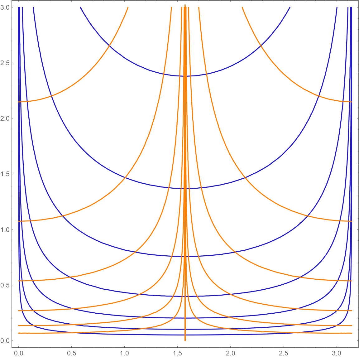
Figure 5. Blue: The level sets of $\lvert\mu\rvert=3r^{2}(c+r^{2})^{1/3}\sin\theta$ in $B=(0,\pi)\times\mathbb{R}^{+}$. Every level set represents an $\operatorname{SU}(2)$-family of $\operatorname{\mathbb{T}}^{2}$-invariant associatives in $M_{P}$. Orange: The level sets of $\nu=2\sqrt{3}r^{2}\cos\theta$. Every level set represents an $S^{2}$ family of $\operatorname{\mathbb{T}}^{3}$-invariant coassociatives in $M_{P}$. The vertical line represents the ones intersecting the zero section, two of these $\operatorname{\mathbb{T}}^{3}$-invariant coassociatives are singular.

It is well-known that all the Bryant–Salamon manifolds are vector bundles with calibrated fibres. In [23], Karigiannis and Lotay considered the $\operatorname{G_{2}}2$ manifolds with associative fibres, namely $\Lambda^{2}_{-}(S^{4})$ and $\Lambda^{2}_{-}(\mathbb{CP}^{2})$, and constructed coassociative fibrations on them. In some sense, they replaced the role of associative and coassociative submanifolds. As a byproduct of Corollary 5.10, we obtain the opposite result, i.e. we construct on the natural coassociative fibre bundle, ${\ooalign{$S$\cr$/$\cr}}(S^{3})$, an associative fibration. We visualize this fibration in Figure 5.

Acknowledgements

The authors wish to express their gratitude to Lorenzo Foscolo and Jason D. Lotay for all the valuable feedback, enlightening conversations and encouragement. The authors are also indebted towards Jakob Stein for explaining to them important aspects of the construction in [17] and for the helpful comments on a first draft of this work.

2. Preliminaries

In this section, we provide the basic definitions and properties of $\operatorname{G_{2}}2$ manifolds, associative submanifolds and coassociative submanifolds. We also discuss some well-knwon preliminary results for blow-up analysis and regularity of calibrated submanifolds.

2.1. $\operatorname{G_{2}}2$ Manifolds

The linear model we consider for a $\operatorname{G_{2}}2$ manifold is $\mathbb{R}^{7}\cong\mathbb{R}^{3}\oplus\mathbb{R}^{4}$ parametrized by $(x_{1},x_{2},x_{3})$ and $(a_{0},a_{1},a_{2},a_{3})$, respectively. On $\mathbb{R}^{7}$, we consider the associative $3$-form $\varphi_{0}$:

$$\varphi_{0}=dx_{1}\wedge dx_{2}\wedge dx_{3}+\sum_{i=1}^{3}dx_{i}\wedge\Omega_{i},$$

where the $\Omega_{i}$s are the standard ASD two-forms of $\mathbb{R}^{4}$ endowed with the Euclidean metric, i.e., $\Omega_{i}=da_{0}\wedge da_{i}-da_{j}\wedge da_{k}$ for $(i,j,k)$ cyclic permuation of $(1,2,3)$. The Hodge dual of $\varphi_{0}$ in $\mathbb{R}^{7}$ is also of great geometrical interest:

$$\ast\varphi_{0}=da_{0}\wedge da_{1}\wedge da_{2}\wedge da_{3}-\sum_{i=1}^{3}dx_{j}\wedge dx_{k}\wedge\Omega_{i},$$

where $(i,j,k)$ is again a positive permutation of $(1,2,3)$.

Since the stabilizer of $\varphi_{0}$ is isomorphic to $\operatorname{G_{2}}2$, the automorphism group of ${\mathbb{O}}$, we can see $(\mathbb{R}^{7},\varphi_{0})$ as the linear model for manifolds with $\operatorname{G_{2}}2$-structure group.

Definition 2.1.

Let $M$ be a manifold and $\varphi$ a $3$-form on $M$. We say that $\varphi$ is a $\operatorname{G_{2}}2$-structure on $M$ if at each point $x\in M$ there exists a linear isomorphism $p_{x}:\mathbb{R}^{7}\to T_{x}M$ which identifies $\varphi_{0}$ with ${\left.\kern-1.2pt\varphi\vphantom{\big{|}}\right|_{x}}$, i.e., $p_{x}^{\ast}{\varphi}=\varphi_{0}$.

A $\operatorname{G_{2}}2$-structure $\varphi$ induces a metric $g_{\varphi}$ and an orientation $\operatorname{vol}_{\varphi}$ on $M$ satisfying:

(2.1) $$(i_{u}\circ\varphi)\wedge(i_{v}\circ\varphi)\wedge\varphi=-6g_{\varphi}(u,v)\operatorname{vol}_{\varphi},$$

for all $u,v\in T_{x}M$ and all $x\in M$. This makes $p_{x}$ an orientation preserving isometry. From $g_{\varphi}$ and $\operatorname{vol}_{\varphi}$, one can also construct the coassociative $4$-form $\ast_{\varphi}\varphi$.

Definition 2.2.

Let $M$ be a manifold and let $\varphi$ be a $\operatorname{G_{2}}2$-structure on $M$. $(M,\varphi)$ is a $\operatorname{G_{2}}2$ manifold if $\varphi$ and $\ast_{\varphi}\varphi$ are closed.

This terminology is justified by the theorem of Fernandez and Gray[14], which states that in this case, the Riemannian holonomy group of $(M,g_{\varphi})$ is contained in $\operatorname{G_{2}}2$. Every $\operatorname{G_{2}}2$ manifold is Ricci-flat.

The octonionic structure on the tangent space equips the tangent bundle with a natural cross product.

Definition 2.3.

Let $(M,\varphi)$ be a manifold with a $\operatorname{G_{2}}2$-structure. The cross product on the tangent bundle $\times_{\varphi}$ is defined as follows:

$$\times_{\varphi}: TM\times TM\to TM$$

$$(U,V)\to(i_{V}\circ i_{U}\circ\varphi)^{\#},$$

where $\#$ denotes the Riemannian musical isomorphism.

2.2. Associatives and coassociatives submanifolds

Harvey and Lawson [19] showed that $\varphi$ and $\ast\varphi$ have co-mass equal to one. It follows that, if $(M,\varphi)$ is a $\operatorname{G_{2}}2$ manifold, then, $\varphi$ and $\ast\varphi$ are calibrations.

Definition 2.4.

Let $F\subset(\mathbb{R}^{7},\varphi_{0})$ be a $3$-dimensional vector subspace. $F$ is an associative plane if ${\left.\kern-1.2pt\varphi_{0}\vphantom{\big{|}}\right|_{F}}=\operatorname{vol}_{F}$. A submanifold $L$ of a $\operatorname{G_{2}}2$ manifold $(M,\varphi)$ is associative if it is calibrated by $\varphi$, i.e. for every $x\in L$ the subspace $T_{x}L$ is an associative plane in $T_{x}M$.

Definition 2.5.

Let $F\subset(\mathbb{R}^{7},\varphi_{0})$ be a $4$-dimensional vector subspace. $F$ is a coassociative plane if ${\left.\kern-1.2pt\ast\varphi_{0}\vphantom{\big{|}}\right|_{F}}=\operatorname{vol}_{F}$. A submanifold $\Sigma$ of a $\operatorname{G_{2}}2$ manifold $(M,\varphi)$ is coassociative if it is calibrated by $\ast\varphi$, i.e. for every $x\in\Sigma$ the subspace $T_{x}\Sigma$ is a coassociative plane in $T_{x}M$.

Remark 2.6.

A submanifold $\Sigma$ is associative or coassociative if and only if $T_{p}\Sigma$ is an associative or a coassociative plane of $(\mathbb{R}^{7},\varphi_{0})$ for every $x\in\Sigma$ under the isomorphism $p_{x}$.

We now state some well-known properties of associative and coassociative planes which will be useful in the discussion below.

Proposition 2.7 (Harvey and Lawson [19]).

Let $F\subset(\mathbb{R}^{7},\varphi_{0})$ be a $3$-dimensional subspace. Then, the following are equivalent:

1. $F$ is an associative plane,

2. $F^{\perp}$ is a coassociative plane,

3. if $u,v\in F$, then, $u\times_{\varphi_{0}}v\in F$,

4. if $u\in F$ and $v\in F^{\perp}$, then, $u\times_{\varphi_{0}}v\in F^{\perp}$,

5. if $u,v\in F^{\perp}$, then, $u\times_{\varphi_{0}}v\in F$,

6. if $u,v,w\in F$, then, $i_{w}\circ i_{v}\circ i_{u}\ast_{\varphi_{0}}\varphi_{0}=0$,

7. if $u,v,w\in F^{\perp}$, then, $i_{w}\circ i_{v}\circ i_{u}\varphi_{0}=0$.

Moreover, it follows that for every $u,v$ linearly independent vectors of $\mathbb{R}^{7}$ there exists a unique associative plane containing them. Analogously, if $u,v,w$ are linearly independent vectors of $\mathbb{R}^{7}$ such that $\varphi_{0}(u,v,w)=0$ there exists a unique coassociative plane containing them.

We can translate this statement to the tangent space $(T_{x}M,{\left.\kern-1.2pt\varphi\vphantom{\big{|}}\right|_{x}})$ of a $\operatorname{G_{2}}2$ manifold through $p_{x}$. In particular, the Cartan-Kähler theorem yields the Harvey–Lawson local existence and uniqueness theorem [19, Section IV.4].

Inspired by [23, 39], we consider a definition of calibrated fibrations where fibres are allowed to be singular and to intersect.

Definition 2.8.

Let $(M,\alpha)$ be a $n$-manifold with a $k$-calibration $\alpha$. $M$ admits an $\alpha$-calibrated fibration if there exists a family of $\alpha$-calibrated submanifolds $N_{b}$ (possibly singular) parametrized by a $(n-k)$-dimensional space $\mathcal{B}$ satisfying the following properties:

• $M$ is covered by the family $\{N_{b}\}_{b\in\mathcal{B}}$,

• there exists an open dense set $\mathcal{B}^{\circ}\subset\mathcal{B}$ such that $N_{b}$ is smooth for all $b\in\mathcal{B}^{\circ}$,

• there exists an open dense subset $M^{\prime}\subset M$, a submanifold $\mathcal{B}^{\prime}\subset\mathcal{B}$ and a smooth genuine fibre bundle $\pi:M^{\prime}\to\mathcal{B}^{\prime}$ with fibre $N_{b}$ for all $b\in\mathcal{B}$.

Remark 2.9.

$M\setminus M^{\prime}$ is the set where the calibrated submanifolds can intersect and can be singular. When we restrict the calibrated submanifolds to $M\setminus M^{\prime}$, these can cease to be complete and they can have a different topology from the original ones.

3. $\operatorname{G_{2}}2$ manifolds with $\operatorname{\mathbb{T}}^{2}\times\operatorname{SU}(2)$-symmetry

In this section, we consider a $\operatorname{G_{2}}2$ manifold $(M,\varphi)$ with a structure-preserving $\operatorname{\mathbb{T}}^{2}\times\operatorname{SU}(2)$-action of cohomogeneity two, i.e. the maximal dimension achieved by the orbits is $5$.

3.1. $\operatorname{\mathbb{T}}^{2}\times\operatorname{SU}(2)$-symmetry

To understand the action of $\operatorname{\mathbb{T}}^{2}\times\operatorname{SU}(2)$ on $M$, let $\Gamma$ be the kernel of the homomorphism $\operatorname{\mathbb{T}}^{2}\times\operatorname{SU}(2)\to\mathrm{Aut}(M)$, which is discrete by assumption. Once we rewrite it as $\Gamma=\{(a_{i},b_{i})\in\operatorname{\mathbb{T}}^{2}\times\operatorname{SU}(2):i\in I\}$, we define $\Gamma_{1}:=\{a\in\operatorname{\mathbb{T}}^{2}:(a,\mathrm{Id}_{\operatorname{SU}(2)})\in\Gamma\}$ and $\Gamma_{2}:=\{b\in\operatorname{SU}(2):(\mathrm{Id}_{\operatorname{\mathbb{T}}^{2}},b)\in\Gamma\}$, which are subgroups of $\operatorname{\mathbb{T}}^{2}$ and $\operatorname{SU}(2)$ respectively.

Consider the $\operatorname{\mathbb{T}}^{2}$ action on $M$ given by $\operatorname{\mathbb{T}}^{2}\times\mathrm{Id}_{\operatorname{SU}(2)}\subset\operatorname{\mathbb{T}}^{2}\times{\operatorname{SU}(2)}$. Since

$$\Gamma_{1}\times\mathrm{Id}_{\operatorname{SU}(2)}=(\operatorname{\mathbb{T}}^{2}\times\mathrm{Id}_{\operatorname{SU}(2)})\cap\Gamma,$$

we see that the action of $\operatorname{\mathbb{T}}^{2}/\Gamma_{1}$ is effective, and, as $\operatorname{\mathbb{T}}^{2}/\Gamma_{1}$ is diffeomorphic to $\operatorname{\mathbb{T}}^{2}$, we can assume, without loss of generality, that $\Gamma_{1}$ is trivial and that the action of $\operatorname{\mathbb{T}}^{2}\cong\operatorname{\mathbb{T}}^{2}\times\mathrm{Id}_{\operatorname{SU}(2)}$ is effective. We denote by $\mathcal{S}$ the singular set of this action, i.e. the complement of the principal set with respect to this action.

Analogously, we have an $\operatorname{SU}(2)$-action on $M$ given by $\operatorname{SU}(2)\cong\mathrm{Id}_{\operatorname{\mathbb{T}}^{2}}\times\operatorname{SU}(2)\subset\operatorname{\mathbb{T}}^{2}\times\operatorname{SU}(2)$, which induces an effective action of $\operatorname{SU}(2)/\Gamma_{2}$. The singular set of this action is denoted by $\tilde{\mathcal{S}}$.

Remark 3.1.

Observe that $\Gamma$ does not need to be equal to $\Gamma_{1}\times\Gamma_{2}$. For instance, if $\Gamma=\{\pm(1,1)\}$, then, $\Gamma_{1}$ and $\Gamma_{2}$ are trivial.

Now, we show that $\Gamma$ is in the center of $\operatorname{\mathbb{T}}^{2}\times\operatorname{SU}(2)$: $Z(\operatorname{\mathbb{T}}^{2}\times\operatorname{SU}(2))=\operatorname{\mathbb{T}}^{2}\times\{\pm 1\}$.

Lemma 3.2.

Let $x\in M$ such that the stabilizer $(\operatorname{\mathbb{T}}^{2}\times\operatorname{SU}(2))_{x}$ is discrete. Then, it is a subgroup of the center $Z(\operatorname{\mathbb{T}}^{2}\times\operatorname{SU}(2))$.

Proof.

We show that the adjoint representation of $(\operatorname{\mathbb{T}}^{2}\times\operatorname{SU}(2))_{x}$ on $\mathfrak{t}^{2}\oplus\mathfrak{su}(2)$ is trivial, which implies the statement by naturality of the exponential map.

Let $N=\nu_{x}$ be the normal space at $x$ of the $\operatorname{\mathbb{T}}^{2}\times\operatorname{SU}(2)$-orbit, whose tangent space is identified with $\mathfrak{t}^{2}\oplus\mathfrak{su}(2)$ in the usual manner. Then, the representation of $(\operatorname{\mathbb{T}}^{2}\times\operatorname{SU}(2))_{x}$ on $T_{x}M$ splits as

(3.1) $$T_{x}M=\mathfrak{t}^{2}\oplus\mathfrak{su}(2)\oplus N,$$

and coincides with the adjoint representation on the $\mathfrak{t}^{2}\oplus\mathfrak{su}(2)$ part. Being abelian, the action on $\mathfrak{t}^{2}$ is trivial and the same holds for the cross product of the $\mathfrak{t}^{2}$-generators, which spans a linear subspace $N_{1}$ of $N$ by Eq. 3.6. Note that we used that the action of $(\operatorname{\mathbb{T}}^{2}\times\operatorname{SU}(2))_{x}$ preserves the $\operatorname{G_{2}}2$-structure. Denote by $N_{2}$ the orthogonal complement of $N_{1}$ in $N$, which is invariant under the action. Being an isometry, every element $g\in(\operatorname{\mathbb{T}}^{2}\times\operatorname{SU}(2))_{x}$ acts on $N_{2}$ by multiplication of $\lambda_{g}$, where $\lambda_{g}\in\{-1,+1\}$.

Finally, we show that $\lambda_{g}$ cannot be $-1$. In order to do so, we consider the map $(\mathfrak{t}^{2}\oplus N_{1})\otimes N_{2}\to\mathfrak{su}(2)$ which is the composition of the cross product and the projection onto the $\mathfrak{su}(2)$ component in the splitting given by Eq. 3.1. Since $\mathfrak{t}^{2}\oplus N_{1}$ is an associative subspace, this map is an isomorphism of representations. Hence, $g$ acts on $\mathfrak{su}(2)$ by multiplication of $\lambda_{g}$. We conclude because there is no element in $\operatorname{\mathbb{T}}^{2}\times\operatorname{SU}(2)$ whose adjoint action on $\mathfrak{su}(2)$ is multiplication by $-1$. ∎

Corollary 3.3.

Since $\operatorname{\mathbb{T}}^{2}\times\operatorname{SU}(2)$ acts with cohomogeneity two, $\Gamma$ is in the centre of $\operatorname{\mathbb{T}}^{2}\times\operatorname{SU}(2)$. Hence, $\operatorname{SU}(2)/\Gamma_{2}$ is either $\operatorname{SU}(2)$ or $\operatorname{SO}(3)$.

Corollary 3.4.

The principal stabilizer of $(\operatorname{\mathbb{T}}^{2}\times\operatorname{SU}(2))/\Gamma$ is trivial.

Proof.

As a consequence of Lemma 3.2, all principal stabilizer subgroups are not only conjugate, but equal to each other. Since the action is effective after the quotient, the principal stabilizer needs to be trivial. ∎

From now on, we consider the action of $G:=(\operatorname{\mathbb{T}}^{2}\times\operatorname{SU}(2))/\Gamma\subset\operatorname{Aut}(M,\varphi)$, and we denote by $M_{P}$ its principal set. This is going to greatly simplify our arguments, indeed, the $G$-action is effective and with trivial principal stabilizer.

We will make use of two additional actions induced from the original $\operatorname{\mathbb{T}}^{2}\times\operatorname{SU}(2)$. Let $\tilde{\Gamma}_{1}:=\{a_{i}:(a_{i},b_{i})\in\Gamma\}$ and let $\tilde{\Gamma}_{2}:=\{b_{i}:(a_{i},b_{i})\in\Gamma\}$, which is either trivial or $\{\pm 1\}$ by Corollary 3.3. We state the following lemma without proof.

Lemma 3.5.

Let $\operatorname{\mathbb{T}}^{2}\cong{\operatorname{\mathbb{T}}^{2}}\times\mathrm{Id}_{\operatorname{SU}(2)}$ acting on $M$. Then, there exists an induced action of $G^{\operatorname{\mathbb{T}}^{2}}:=\operatorname{\mathbb{T}}^{2}/\tilde{\Gamma}_{1}$ on $M_{P}/(\operatorname{SU}(2)/\Gamma_{2})$ which is free. In particular, $M_{P}/(\operatorname{SU}(2)/\Gamma_{2})$ becomes a principal $G^{\operatorname{\mathbb{T}}^{2}}$-bundle over $B:=M_{P}/G$. Similarly, there exists a $G^{\operatorname{SU}(2)}:=\operatorname{SU}(2)/\tilde{\Gamma}_{2}$ action induced by $\operatorname{SU}(2)\cong\mathrm{Id}_{\operatorname{\mathbb{T}}^{2}}\times{\operatorname{SU}(2)}$ on $M_{P}/\operatorname{\mathbb{T}}^{2}$ which is free. As before, $M_{P}/\operatorname{\mathbb{T}}^{2}$ becomes a principal $G^{\operatorname{SU}(2)}$-bundle over $B$.

The various group quotient are summarised in the following diagram:

$$\leavevmode\hbox to191.46pt{\vbox to84.68pt{\text{[drawing]}}}. {M_{P}} {M_{P}/{(\mathrm{SU}(2)/{\Gamma_{2}})}} {M_{P}/{\mathbb{T}^{2}}} {B} \scriptstyle{/{(\mathrm{SU}(2)/{\Gamma_{2}})}} \scriptstyle{/\mathbb{T}^{2}} \scriptstyle{/G} \scriptstyle{/G^{\mathbb{T}^{2}}} \scriptstyle{/G^{\mathrm{SU}(2)}} {M_{P}} {M_{P}/{(\mathrm{SU}(2)/{\Gamma_{2}})}} {M_{P}/{\mathbb{T}^{2}}} {B} \scriptstyle{/{(\mathrm{SU}(2)/{\Gamma_{2}})}} \scriptstyle{/\mathbb{T}^{2}} \scriptstyle{/G} \scriptstyle{/G^{\mathbb{T}^{2}}} \scriptstyle{/G^{\mathrm{SU}(2)}}$$

3.2. The stratification

Applying the orbit type stratification theorem and the principal orbit type theorem to our setting, where $G=(\operatorname{\mathbb{T}}^{2}\times\operatorname{SU}(2))/\Gamma$ acts effectively on $M$, we see that $M$ decomposes as the union of $G$-orbit types, and there exists one of them which is open and dense in $M$. In this subsection, we study the geometry of the $G$-action to understand this stratification.

To simplify our notation, we fix a point $x\in M$ and denote by $T$ the tangent space of $Gx$ at $x$ and by $N$ its normal space, i.e. the orthogonal complement of $T$ in $T_{x}M$.

In the discussion of the stratification, we will need the following lemma:

Lemma 3.6.

Let $\operatorname{\mathbb{T}}^{2}$ be a maximal torus in $\operatorname{G_{2}}2$. Then, the representation of $\operatorname{\mathbb{T}}^{2}$ on $\mathbb{R}^{7}$ splits as $V\oplus W_{1}\oplus W_{2}\oplus W_{3}$. Where $V$ is $1$-dimensional and each $W_{i}$ is $2$-dimensional. Each of $V\oplus W_{i}$ is an associative subspace.

Recall that $\mathcal{S}$ is the singular set of the $\operatorname{\mathbb{T}}^{2}$-action and, as a consequence of the following theorem, it is also set where the generators of the $\operatorname{\mathbb{T}}^{2}$-component are linearly dependent, i.e. there are no exceptional orbits (cfr. [34, Lemma 2.6]).

Theorem 3.7.

The dimension of the stabilizer $G_{x}$ is not bigger than $4$, and,

• if $\dim(G_{x})=0$, then, $G_{x}$ is trivial, i.e. there are no exceptional orbits,

• if $\dim(G_{x})=1$, then, $x\notin\mathcal{S}$ and $G_{x}$ is isomorphic to $\operatorname{SO}(2)$. The action of $G_{x}$ on $N$ splits as $N_{1}\oplus N_{2}$ with $\dim(N_{1})=1,\dim(N_{2})=2$ where $G_{x}$ acts trivially on $N_{1}$ and faithfully by rotations on $N_{2}$,

• if $\dim(G_{x})=2$, then, $x\in S$ and the identity component of $G_{x}$ is isomorphic to $\operatorname{\mathbb{T}}^{2}$ and acts as a maximal torus in $\operatorname{U}(2)$ on $N$. The $G$-orbit $Gx$ is an associative submanifold of $M$,

• if $\dim(G_{x})=3$, then, $x\notin S$ and $G_{x}$ is diffeomorpic to $\operatorname{SU}(2)$. The action of $G_{x}$ on $N$ leaves a $1$-dimensional subspace $N_{1}\subset N$ invariant and acts on the orthogonal complement $N_{2}$ via the standard embedding $\operatorname{SU}(2)\to\operatorname{SO}(4)$,

• if $\dim(G_{x})=4$, then, $x\in S$ and the identity component of $G_{x}$ is isomorphic to $\operatorname{U}(2)$. The action on the normal bundle $N$ is via the embedding

  $$U(2)\to\operatorname{SU}(3),\quad A\mapsto\begin{pmatrix}A&0\\ 0&\det{A}^{-1}\end{pmatrix}.$$

Consequently, the singular orbit set can be decomposed into $\mathcal{S}_{1}\cup\mathcal{S}_{2}\cup\mathcal{S}_{3}\cup\mathcal{S}_{4}$ where $\mathcal{S}_{i}$ is the set of points with $i$-dimensional stabilizer.

Proof.

The first part of the proposition follows from the fact that the rank of $\mathfrak{t}^{2}\oplus\mathfrak{su}(2)$ is three, while the rank of $\mathfrak{g}_{2}$ is two. Hence, since $G_{x}\subset\operatorname{G_{2}}2$ under the identification of $(T_{x}M,\varphi_{x})\cong(\mathbb{R}^{7},\varphi_{0})$, the dimension of $G_{x}$ cannot be equal to 5.

By the slice theorem, a neighbourhood of $Gx$ is equivariantly diffeomorphic to a neighbourhood of the zero section of $G\times_{G_{x}}N.$ It follows that the representation of $G_{x}$ on $N$ is faithful. Indeed, every neighbourhood of the orbit $Gx$ intersects $M_{P}$, on which $G_{x}$ acts freely because of Corollary 3.4.

If $\mathrm{dim}(G_{x})=0$, then, an argument similar to the one used for Lemma 3.2 shows that $G_{x}$ acts trivially on $N$. This means that $G_{x}$ is trivial by the faithfullness of the $G_{x}$-action on $N$.

We now consider the case $\mathrm{dim}(G_{x})=1$ and $x\in\mathcal{S}$. This means that $\bar{G}_{x}=G_{x}\cap(\operatorname{\mathbb{T}}^{2}\times\mathrm{Id}_{\operatorname{SU}(2)})/\Gamma$ is not trivial and, being a subgroup of $(\operatorname{\mathbb{T}}^{2}\times\mathrm{Id}_{\operatorname{SU}(2)})/\Gamma$, it acts trivially on $T\cong\mathfrak{g}/\mathfrak{g}_{x}$. Since the cross-product restricted to any $4$-dimensional subspace generates $T_{x}M$, we deduce that $\bar{G}_{x}$ acts trivially on all of $T_{x}M$. This is a contradiction as $\bar{G}_{x}\leq G_{x}$ and hence it has to act faithfully on $N$. We have shown that if $\mathrm{dim}(G_{x})=1$, then, $x\notin\mathcal{S}$. So it remains to show that $G_{x}$ is isomorphic to $S^{1}$. Since $x\notin\mathcal{S}$ the intersection of $\mathfrak{t}^{2}\oplus\{0\}\subset\mathfrak{t}^{2}\oplus\mathfrak{su}(2)$ with $\mathfrak{g}_{x}$ is trivial. This means that $\mathfrak{g}/\mathfrak{g}_{x}$ splits into $\mathfrak{t}^{2}$, on which $G_{x}$ acts trivially, and a $2$-dimensional subspace $\mathfrak{m}$. As before, the normal space splits into $N_{1}\oplus N_{2}$, where $N_{1}$ is spanned by the cross product on $\mathfrak{t}^{2}$ and $N_{2}$ is its orthogonal complement in $N$. So $G_{x}$ acts trivially on $N_{1}$. To summarise, the action of $G_{x}$ on $T_{x}M$ splits as

$$T_{x}M=\mathfrak{t}^{2}\oplus\mathfrak{m}\oplus N_{1}\oplus N_{2}.$$

The action of $G_{x}$ is isometric and faithful on the $2$-dimensional space $N_{2}$. So, $G_{x}$ is either isomorphic to $\operatorname{SO}(2)$ or to $\mathrm{O}(2)$. In the latter case, there is an element $\tau$ of order two and a subspace $N_{3}\subset N_{2}$ that is fixed by $\tau$. The cross products of $\mathfrak{t}^{2}\oplus N_{1}\oplus N_{3}$ generate all of $T_{x}M$ so that $\tau$ acts trivially on all of $T_{x}M$. This is impossible since the action on $N$ must be faithful.

When $\mathrm{dim}(G_{x})=2$, we first assume by contradiction that $x\notin\mathcal{S}$. Consider the Lie algebra homomorphism $\psi\colon\mathfrak{g}_{x}\to\mathfrak{su}(2)$ coming from the projection $\mathfrak{t}^{2}\oplus\mathfrak{su}(2)\to\mathfrak{su}(2)$. The image of $\psi$ would be a $2$-dimensional Lie subalgebra of $\mathfrak{su}(2)$ which does not exist. It follows that $x\in\mathcal{S}$ and the identity component of $G_{x}$ is isomorphic to $\operatorname{\mathbb{T}}^{2}$. Since the action of the identity component of $G_{x}$ splits at $T\oplus N$, we can apply Lemma 3.6 to see that $T$ is isomorphic to $V$ plus one of the $W_{i}$, for convenience say $W_{1}$, and $N$ to the sum of $W_{2}\oplus W_{3}$ and the statement follows.

We now deal with the $\mathrm{dim}(G_{x})=3$ case. Consider the Lie algebra homomorphism $\psi\colon\mathfrak{g}_{x}\to\mathfrak{su}(2)$ as above. The image of $\psi$ is a Lie subalgebra of $\mathfrak{su}(2)$, hence, it is either $\mathfrak{su}(2)$ or a $1$-dimensional subalgebra. The second case is impossible, indeed, the condition implies $\mathfrak{t}^{2}\oplus\{0\}\subset\mathfrak{g}_{x}$, but $\mathfrak{g}_{x}$ also intersects $\mathfrak{su}(2)$ in a $1$-dimensional subspace, so $\mathfrak{g}_{x}\cong\mathfrak{t}^{2}\oplus\psi(\mathfrak{g}_{x})\cong\mathfrak{t}^{3}$. This is a contradiction since $\mathfrak{g}_{x}$ is a subalgebra of $\mathfrak{g}_{2}$, which has rank two. So $\psi$ is surjective, which means that $\mathfrak{g}_{x}$ intersects $\mathfrak{t}^{2}\oplus\{0\}$ transversally. It remains to show that $G_{x}$ is diffeomorphic to $\operatorname{SU}(2)$, which also implies that $x\notin\mathcal{S}$. As before, $G_{x}$ acts trivially on $\mathfrak{g}/\mathfrak{g}_{x}=\mathfrak{t}^{2}$. The element $U_{1}\times U_{2}$ lies in $N$ and spans a $1$-dimensional subspace $N_{1}$ on which $G_{x}$ acts trivially too. On the orthogonal complement $N_{2}$ of $N_{1}$ in $N$ the action of $G_{x}$, is faithful. So $G_{x}$ acts trivially on an associative three-plane, which means $G_{x}$ is a subgroup of $\operatorname{SU}(2)$. Since $G_{x}$ is $3$-dimensional, it is isomorphic to $\operatorname{SU}(2)$ and the action on $N_{2}$ is isomorphic to the standard action of $\operatorname{SU}(2)$ on $\mathbb{C}^{2}$.

Finally, we consider $\dim(G_{x})=4$. Similarly as above, we can show that $T$ is the span of $U_{1}$ and $U_{2}$, it is $1$-dimensional, and it is fixed by $G_{x}$. The subgroup of $\operatorname{G_{2}}2$ that fixes a $1$-dimensional subspace is $\operatorname{SU}(3)$. So, the action of $G_{x}$ on the $6$-dimensional normal space $N$ defines an embedding $G_{x}\to\operatorname{SU}(3)$, yielding a special unitary representation of $G_{x}$ on $\mathbb{C}^{3}$. We first show that, when restricted to the identity component, this representation must be reducible. Indeed, every $4$-dimensional Lie subalgebra of $\mathfrak{g}$ is isomorphic to $\mathfrak{u}(2)=\mathfrak{su}(2)\oplus\mathfrak{u}(1)$. Since $G_{x}$ is compact, it suffices to show that every complex $3$-dimensional special unitary representation of $\operatorname{SU}(2)\times\operatorname{U}(1)$ is reducible. To see this, denote by $V_{k}$ the unique $k$-dimensional irreducible representation of $\operatorname{SU}(2)$ and by $W_{m}$ the representation of $\operatorname{U}(1)$ on $\mathbb{C}$ with weight $m$. All irreducible representations of the direct product $\operatorname{SU}(2)\times\operatorname{U}(1)$ are of the form $V_{k}\otimes W_{m}$. The $3$-dimensional of these, $V_{3}\otimes W_{m}$, are not special unitary. Since the representation is faithful and special unitary, we conclude that it must be $(V_{2}\otimes W_{1})\oplus W_{-2}$, i.e. of the desired form. Moreover, the element $(-1,-1)$ acts trivially, so the identity component of $G_{x}$ must be $(\operatorname{SU}(2)\times\operatorname{U}(1))/{\mathbb{Z}_{2}}\cong\operatorname{U}(2)$. ∎

Note that the third part of the theorem implies that either $\mathcal{S}_{3}=\emptyset$ or $G^{\operatorname{SU}(2)}=\operatorname{SU}(2)$.

Corollary 3.8.

The singular set of the $\operatorname{\mathbb{T}}^{2}$-action is $\mathcal{S}=\mathcal{S}_{2}\cup\mathcal{S}_{4}$.

The following statement follows from the slice theorem and by how $G_{x}$ acts on the normal bundles in Theorem 3.7.

Proposition 3.9.

Each $\mathcal{S}_{i}$ is either empty or a smooth embedded submanifold of dimension:

$$\dim(\mathcal{S}_{1})=5,\hskip 5.0pt\dim(\mathcal{S}_{2})=3,\hskip 5.0pt\dim(\mathcal{S}_{3})=3,\hskip 5.0pt\dim(\mathcal{S}_{4})=1.$$

Moreover, each connected component of $\mathcal{S}_{2}$ and $\mathcal{S}_{4}$ are $G$-orbits.

Figure 1. Representation of how the different $\mathcal{S}_{i}$s intersect.

Remark 3.10.

Note that the stratification induced by $\{\mathcal{S}_{i}\}$ is not the one of the orbit type stratification theorem, as there could be different orbit types of the same dimension. However, we have seen in Proposition 3.9 that the tangent space of each $\mathcal{S}_{i}$ is spanned by the tangent space of the orbit and possibly $U_{1}\times U_{2}$. Since the flow of $U_{1}\times U_{2}$ preserves the orbit type (see Lemma 5.2), the orbit type is unchanged along every connected component of each $\mathcal{S}_{i}$ and, hence, we can reconstruct one stratification from the other.

3.3. Multi-moment maps

In [32] and [33], Madsen and Swann extended the classical notion of moment maps for symplectic manifolds to any closed geometry $(X,\alpha)$, i.e. a manifold $X$ endowed with a closed form $\alpha$. Roughly speaking, the idea is to take generators of a subgroup of $\operatorname{Aut}(X,\alpha)$ and contract them with $\alpha$ to reduce its degree to 1. Now, if these 1-forms are exact they can be integrated to functions that they call multi-moment maps. In order to ensure closedness, Madsen and Swann introduced the notion of kth Lie kernel, which we omit for brevity.

From now on, we assume the $\operatorname{G_{2}}2$ manifold to be simply connected, so that all closed $1$-forms are exact. In this setting, we can describe the components of the multi-moment maps related to $\varphi$ and $\ast\varphi$ in an explicit way.

Remark 3.11.

Observe that it makes sense to consider the multi-moment maps with respect to $\ast\varphi$ as well. Indeed, Eq. 2.1 implies that an action preserving $\varphi$ will also preserve the metric $g_{\varphi}$ and the volume form $\operatorname{vol}_{\varphi}$. Therefore, $\ast\varphi$ will also be preserved.

Let $U_{1},U_{2}$ be the generators of the $\mathfrak{t}^{2}$ component, while $V_{1},V_{2},V_{3}$ are the generators of the $\mathfrak{su}(2)$ component. Clearly, we can choose them to satisfy:

(3.2) $$[U_{l},U_{m}]=0,\hskip 15.0pt[U_{l},V_{i}]=0,\hskip 15.0pt[V_{i},V_{j}]=\epsilon_{ijk}V_{k},$$

for all $l,m=1,2$ and $i,j,k=1,2,3$.

The components of the multi-moment maps with respect to $\varphi$ are defined by:

(3.3) $$d\theta^{l}_{i}:=\varphi(U_{l},V_{i},\cdot),\hskip 15.0ptd\nu:=\varphi(U_{1},U_{2},\cdot),$$

where $l=1,2$, $i=1,2,3$.

The components of the multi-moment maps with respect to $\ast\varphi$ are defined by:

(3.4) $$d\mu_{i}:=\ast\varphi(U_{1},U_{2},V_{i},\cdot),\hskip 15.0ptd\eta:=\ast\varphi(V_{1},V_{2},V_{3},\cdot),$$

where $i=1,2,3$.

As a reality check, one can show that the one-forms given on the right-hand-side are all closed.

Lemma 3.12.

The multi-moment maps $\mu$ and $\theta$ can be computed explicitly and, up to additive constants, have the form:

(3.5) $$\mu_{k}=-\ast\varphi(U_{1},U_{2},V_{i},V_{j}),\hskip 15.0pt\theta_{k}^{l}=-\varphi(U_{l},V_{i},V_{j})$$

i.e., $d\mu_{k}=\ast\varphi(U_{1},U_{2},V_{k},\cdot)$ and $d\theta_{k}^{l}=\varphi(U_{l},V_{k},\cdot)$, where $(i,j,k)$ is a cyclic permutation of $(1,2,3)$.

Proof.

The proof is a straightforward application of Cartan’s formula, the identity $[\mathcal{L}_{X},i_{Y}]=i_{[X,Y]}$ for every vector field $X,Y$ and Eq. 3.2. ∎

Before considering the properties of the multi-moment maps, we state two classical result that we will use throughout the paper.

Lemma 3.13.

Let $M$ be a smooth manifold with an $\operatorname{SU}(2)$ action of generators $V_{1},V_{2},V_{3}$ satisfying $[V_{i},V_{j}]=\epsilon_{ijk}V_{k}$. Then, a smooth function $f\colon M\to\mathbb{R}^{3}$ is equivariant with respect to the action of $\operatorname{SU}(2)$ on $\mathbb{R}^{3}$ via the double cover $\operatorname{SU}(2)\to\operatorname{SO}(3)$ if and only if $f$ satisfies:

$$\mathcal{L}_{V_{i}}f_{j}=\epsilon_{ijk}f_{k}.$$

Lemma 3.14.

Let $M$ be a smooth manifold with the action of a connected Lie group $G$ of generators $U_{1},...,U_{l}$. Then, a smooth function $f\colon M\to\mathbb{R}$ is invariant under the $G$-action if and only if $f$ satisfies:

$$\mathcal{L}_{U_{i}}f=0,$$

for every $i=1,...,l$.

Proposition 3.15.

Let $\nu$ be as in Eq. 3.3, let $\mu:=(\mu_{1},\mu_{2},\mu_{3})$ and $\theta^{l}:=(\theta_{1}^{l},\theta_{2}^{l},\theta_{3}^{l})$ be as in Eq. 3.5. Then, $\nu$ is $\operatorname{\mathbb{T}}^{2}\times\operatorname{SU}(2)$-invariant, $\mu$ and $\theta^{l}$ are ${\operatorname{\mathbb{T}}^{2}}$-invariant and ${\operatorname{SU}(2)}$-equivariant, where ${\operatorname{SU}(2)}$ acts on $\mathbb{R}^{3}$ via the double cover $\operatorname{SU}(2)\to\operatorname{SO}(3)$. Finally, $\eta$ is always $\operatorname{SU}(2)$-invariant and also $\operatorname{\mathbb{T}}^{2}$-invariant if the $\operatorname{SU}(2)/\Gamma_{2}$-action has a singular orbit. Moreover, these functions pass to the appropriate quotients.

Proof.

The $\operatorname{\mathbb{T}}^{2}$-invariance of $\nu,\mu$ is clear from Lemma 3.14 equations Eq. 3.3 and Eq. 3.4, while the $\operatorname{SU}(2)$-equivariance of $\mu$ and $\theta^{l}$ follows from Lemma 3.13 and:

$$\mathcal{L}_{V_{i}}\mu_{j}=\epsilon_{ijk}\mu_{k},\hskip 15.0pt\mathcal{L}_{V_{i}}\theta^{l}_{j}=\epsilon_{ijk}\theta^{l}_{k}.$$

If we show that $\varphi(U_{1},U_{2},V_{i})=0$ for every $i=1,2,3$, then, $\nu$ is $\operatorname{SU}(2)$-invariant and $\theta^{l}$ is $\operatorname{\mathbb{T}}^{2}$-invariant. Cartan’s formula, together with $[\mathcal{L}_{X},i_{Y}]=i_{[X,Y]}$, implies that $d(\varphi(U_{1},U_{2},V_{i}))=0$ and, hence, $\varphi(U_{1},U_{2},V_{i})$ is a constant $c_{i}$. We conclude because:

(3.6) $$0=\mathcal{L}_{V_{j}}c_{i}=V_{j}(\varphi(U_{1},U_{2},V_{i}))=-\varphi(U_{1},U_{2},V_{k})=-c_{k},$$

where we used again Cartan’s formula and Eq. 3.2. Analogously, one can prove that $\eta$ is $\operatorname{\mathbb{T}}^{2}$-invariant if the $\operatorname{SU}(2)/\Gamma_{2}$-action has a singular orbit. We conclude as $\eta$ is obviously $\operatorname{SU}(2)$-invariant. ∎

Since the $\operatorname{\mathbb{T}}^{2}\times\operatorname{SU}(2)$-action is structure preserving, and in particular, its generators are killing vector fields, we can obtain the following result. Recall that the Lie derivative of a killing vector field commutes with musical isomorphisms.

Corollary 3.16.

Let $\nu$ be as in Eq. 3.3, let $\mu:=(\mu_{1},\mu_{2},\mu_{3})$ and $\theta^{l}:=(\theta_{1}^{l},\theta_{2}^{l},\theta_{3}^{l})$ be as in Eq. 3.5. Then, $\nabla\nu=U_{1}\times U_{2}$ and $\nabla\lvert\mu\rvert^{2}$ are $\operatorname{\mathbb{T}}^{2}\times\operatorname{SU}(2)$-invariant, while $\nabla\eta$ is always $\operatorname{SU}(2)$-invariant and also $\operatorname{\mathbb{T}}^{2}$-invariant if the $\operatorname{SU}(2)/\Gamma_{2}$-action has a singular orbit. Moreover, these vector fields pass to the appropriate quotients.

Remark 3.17.

As an abuse of notation, we will use the same symbol for both the invariant functions (or vector fields) in the total space and in the quotients.

We are also able to locate the zero set of the multi-moment map of $\mu$ in terms of the stratification given in Theorem 3.7.

Corollary 3.18.

The zero set of $\mu$ satisfies:

$$\mathcal{S}_{2}\cup\mathcal{S}_{3}\cup\mathcal{S}_{4}\subset\mu^{-1}(0)\subset\mathcal{S}_{1}\cup\mathcal{S}_{2}\cup\mathcal{S}_{3}\cup\mathcal{S}_{4}.$$

Proof.

The statement follows from Theorem 3.7 and and that the two-form $\ast\varphi(U_{1},U_{2},\cdot,\cdot)$ does not vanish on any $3$-dimensional subspace, orthogonal to $U_{1}\times U_{2}$. ∎

4. Local characterization of $\operatorname{G_{2}}2$ manifolds with $\operatorname{\mathbb{T}}^{2}\times\operatorname{SU}(2)$-symmetry

Any smooth hypersurface in a torsion-free $\operatorname{G_{2}}2$ manifold carries a half-flat $\operatorname{SU}(3)$-structure [12]. Moreover, under the real-analytic condition, one can locally reverse this procedure through Hitchin’s flow [21]. In our setup, it is natural to take a level set of $\nu$ as the given hypersurface. Indeed, it inherits the $\operatorname{\mathbb{T}}^{2}\times\operatorname{SU}(2)$-symmetry and have $U_{1}\times U_{2}$ as a normal vector field. The main result of this subsection, Theorem 4.8, is to describe half-flat $\operatorname{SU}(3)$-structures with cohomogeneity one $\operatorname{\mathbb{T}}^{2}\times\operatorname{SU}(2)$-symmetry as a solution of an ODE system.

We proceed in two steps. Firstly, in Section 4.1, we only assume $\operatorname{\mathbb{T}}^{2}$-symmetry and recall from [32] that the $\operatorname{SU}(3)$-structure on the level sets of $\nu$ is described as a $\operatorname{\mathbb{T}}^{2}$-bundle over a four manifold $\chi$, with a coherent tri-symplectic structure. Secondly, in Section 4.2, we enhance the symmetry to $\operatorname{\mathbb{T}}^{2}\times\operatorname{SU}(2)$ which implies that the structure on $\chi$ admits a structure-preserving $G^{\operatorname{SU}(2)}$-action. In Proposition 4.5, we show that coherent tri-symplectic structures with this symmetry are the solution of an ODE system.

4.1. The $\operatorname{\mathbb{T}}^{2}$-reduction

Let $(M,\varphi)$ be a $\operatorname{G_{2}}2$ manifold with a structure-preserving $\operatorname{\mathbb{T}}^{2}$-action and singular set $\mathcal{S}$. On $M\setminus\mathcal{S}$, the level sets of $\nu$ are hypersurfaces oriented by $\nabla\nu=U_{1}\times U_{2}$. The $\operatorname{\mathbb{T}}^{2}$-action passes to the level sets of $\nu$ and, hence, it endows $\nu^{-1}(t)$ with a $\operatorname{\mathbb{T}}^{2}$-bundle structure over $\nu^{-1}(t)/\operatorname{\mathbb{T}}^{2}$, which inherits the following additional structure (cfr. [32]).

Definition 4.1.

A $4$-manifold $\chi$ has a coherent tri-symplectic structure if it admits three symplectic forms $\overline{\sigma}_{0},\overline{\sigma}_{1},\overline{\sigma}_{2}$ such that $\overline{\sigma}_{0}\wedge\overline{\sigma}_{i}=0$ for $i=1,2$, $\overline{\sigma}_{0}\wedge\overline{\sigma}_{0}$ is a volume form of $\chi$ and the matrix $Q:=(Q_{ij})_{i,j=1,2}$ defined by $\overline{\sigma}_{i}\wedge\overline{\sigma}_{j}=Q_{ij}\overline{\sigma}_{0}\wedge\overline{\sigma}_{0}$ is positive definite.

The forms defining this structure on $\nu^{-1}(t)/\operatorname{\mathbb{T}}^{2}$ are:

(4.1) $$\overline{\sigma}_{0}=\ast\varphi(U_{1},U_{2},\cdot,\cdot),\quad\overline{\sigma}_{1}=\varphi(U_{1},\cdot,\cdot),\quad\overline{\sigma}_{2}=\varphi(U_{2},\cdot,\cdot),$$

where $U_{1},U_{2}$ are two generators of the $\operatorname{\mathbb{T}}^{2}$-action.

Conversely (see [32, Theorem 6.10]), assuming real analyticity, one can locally reconstruct a $\operatorname{G_{2}}2$ manifold with $\operatorname{\mathbb{T}}^{2}$-symmetry from a coherent tri-symplectic four manifold $\chi$, equipped with a closed two form $F\in\Omega^{2}(\chi,\mathbb{R}^{2})$ with integral periods and whose self-dual part $F_{+}$ satisfies the orthogonality condition:

(4.2) $$F_{+}=(\bar{\sigma}_{1},\bar{\sigma}_{2})A,$$

for some $A\in\operatorname{GL}(2,\mathbb{R})$ such that $\mathrm{Tr}(AQ)=0$. These conditions guarantee that $F_{+}$ is the curvature form of a $\operatorname{\mathbb{T}}^{2}$-bundle $N$ over $\chi$. The $\operatorname{G_{2}}2$-structure is then constructed from $N$ by running rescaled Hitchin’s flow. The resulting $\operatorname{G_{2}}2$-structure yields a moment map $\nu$ of which $N$ is a level set and rescaled Hitchin’s flow evolves $N$ into other level sets of $\nu$.

When the symmetry is enhanced to $\operatorname{\mathbb{T}}^{2}\times\operatorname{SU}(2)$, the remaining $G^{\operatorname{SU}(2)}$-symmetry passes to the quotient $\chi$ and preserves its coherent tri-symplectic structure (see Eq. 4.1). We now describe such four manifolds with a free $G^{\operatorname{SU}(2)}$-symmetry.

4.2. On $4$-manifolds with coherent symplectic triple and $G^{\operatorname{SU}(2)}$-symmetry

Let $\chi$ be a coherent symplectic $4$-manifold with a $G^{\operatorname{SU}(2)}$ structure-preserving free action generated by the vector fields $V_{1},V_{2},V_{3}$ satisfying $[V_{i},V_{j}]=\epsilon_{ijk}V_{k}$. Since the action is structure-preserving, we have that $\mathcal{L}_{V_{i}}\bar{\sigma}_{j}=0$, therefore, $Q$ is $G^{\operatorname{SU}(2)}$-invariant. Moreover, as $Q$ is also positive definite, there exists a unique real symmetric, positive definite $2\times 2$ matrix $T$ such that $T^{-2}=T^{-1}(T^{-1})^{T}=Q$, which is $G^{\operatorname{SU}(2)}$-invariant as well.

Let $\operatorname{vol}_{\chi}:=\frac{1}{2}\bar{\sigma}_{0}\wedge\bar{\sigma}_{0}$ and define the forms $\sigma_{i}:=\sum_{j=1}^{2}T_{ij}\bar{\sigma}_{j}$ for $i=1,2$, which then satisfy $\sigma_{i}\wedge\sigma_{j}=2\delta_{ij}\operatorname{vol}_{\chi}$. Define the metric:

$$g_{\chi}(u,v)\operatorname{vol}_{\chi}=\sigma_{0}\wedge i_{u}\sigma_{1}\wedge i_{v}\sigma_{2},$$

for all $u,v\in T_{x}\chi$ and all $x\in\chi$. With respect to this metric, the vector fields $V_{i}$ are Killing for $g_{\chi}$.

Using the standard cover $\operatorname{SL}(4,\mathbb{R})\to\operatorname{SO}(3,3)$ induced by the map:

$$\Lambda^{2}\otimes\Lambda^{2}\to\Lambda^{4}\cong\mathbb{R},\quad\alpha\otimes\beta\mapsto\alpha\wedge\beta,$$

we show the following lemma.

Lemma 4.2.

There are unique $g_{\chi}$-orthonormal one-forms $\alpha_{i}$ for $i=0,...,3$ such that

(4.3) $$\begin{split}{\sigma}_{0}&=\alpha_{0}\wedge\alpha_{1}+\alpha_{2}\wedge\alpha_{3},\quad{\sigma}_{1}=\alpha_{0}\wedge\alpha_{2}+\alpha_{3}\wedge\alpha_{1},\\ {\sigma}_{2}&=\alpha_{0}\wedge\alpha_{3}+\alpha_{1}\wedge\alpha_{2},\quad\alpha_{0}=\frac{1}{\sqrt{\det{{\hat{g}}_{\chi}}}}\mathrm{vol}_{\chi}(V_{1},V_{2},V_{3},\cdot),\end{split}$$

where $\hat{g}_{\chi}$ is the matrix $(g_{\chi}(V_{i},V_{j}))_{i,j=1,2,3}$.

We define the unit vector field $X:=\alpha_{0}^{\musSharp}$, which satisfies the conditions $\alpha_{0}(X)=1$ and $\alpha_{i}(X)=0$ for $i=1,2,3$, and determines the $\alpha_{i}$s by $\alpha_{i}={\sigma}_{i{-1}}(X,\cdot)$. Consider the two $3\times 3$-matrices:

$$\eta_{ij}:={\sigma}_{i-1}(X,V_{j})=\alpha_{i}(V_{j}),\hskip 10.0pt\tau_{ij}:={\sigma}_{i-1}(V_{k},V_{l}),$$

where $(j,k,l)$ is a positive permutation of $(1,2,3)$. We also define the one-forms $\delta_{0}$ and $\delta_{i}$ for $i=1,2,3$ by:

$$\delta_{0}={\sqrt{\det{\hat{g}_{\chi}}}}\alpha_{0}=\mathrm{vol}_{\chi}(V_{1},V_{2},V_{3},\cdot),\quad\delta_{i}(V_{j})=\delta_{ij},\quad\delta_{i}(X)=0.$$

which satisfies $\alpha_{i}=\sum_{j=1}^{3}\eta_{ij}\delta_{j}.$

Using that $[V_{i},X]=0$, standard computations yield the following.

Lemma 4.3.

The matrix functions $\eta$ and $\tau$ have the following properties

• $\tau=\mathrm{adj}(\eta^{T})$,

• the row vectors of $\tau$ and $\eta$ are $G^{\operatorname{SU}(2)}$-equivariant, and hence, their determinant is $G^{\operatorname{SU}(2)}$-invariant,

• The metric on the vector fields $V_{1},V_{2},V_{3}$, which we called $\hat{g}_{\chi}$, is determined by $\eta$ via:

  (4.4) $$\hat{g}_{\chi}=\eta^{T}\eta,$$

• We have the matrix equation:

  (4.5) $${\sigma}=\frac{1}{\det(\eta)}\delta_{0}\wedge\eta\delta+\mathrm{adj}(\eta)^{T}\bar{\delta},$$

where ${\sigma}=({\sigma}_{1},{\sigma}_{2},{\sigma}_{3})^{T}$, $\delta=(\delta_{1},\delta_{2},\delta_{3})^{T}$, $\bar{\alpha}=(\alpha_{2}\wedge\alpha_{3},\alpha_{3}\wedge\alpha_{1},\alpha_{1}\wedge\alpha_{2})^{T}$ and $\bar{\delta}=(\delta_{2}\wedge\delta_{3},\delta_{3}\wedge\delta_{1},\delta_{1}\wedge\delta_{2})^{T}$

4.3. The differential equation

Now, we deduce how the equations $d\bar{\sigma}_{i}=0$ transform under the given change of frame. We assume that $H^{1}(\chi,\mathbb{R})=0$ so that there is a function $R$ such that $dR=\delta_{0}$. The dual vector field $\partial_{R}$ is equal to ${(\det{\eta})^{-1}}X$, so it satisfies $[\partial_{R},V_{i}]=0$, for every $i=1,2,3$. Morever, by Lemma 4.3 and the commutator relationships for $X$ and $V_{i}$, we deduce that $d\delta=-\bar{\delta}$ and $d(\frac{1}{\det\eta}\delta_{0})=0$.

We recall the following version of Lemma 3.13 in terms of differential forms, which can be proven using Cartan’s formula.

Lemma 4.4.

A smooth function $f\colon\chi\to\mathbb{R}^{3}$ is $\operatorname{SU}(2)$-equivariant if and only if $(df=f\times\delta)\mod\delta_{0},$ for $(f\times\delta)_{i}=\epsilon_{ijk}f_{j}\delta_{k}$.

Consequently, we have

$$d\eta=\eta\times\delta+\frac{\partial\eta}{\partial R}\delta_{0},\quad d\tau{=\tau\times\delta+\frac{\partial\tau}{\partial R}}\delta_{0},$$

where $(\eta\times\delta)_{ij}=(\eta_{i}\times\delta)_{j}$ and $(\tau\times\delta)_{ij}=(\tau_{i}\times\delta)_{j}$, i.e. we are taking the cross products of the rows of $\eta$ with $\delta$. Putting all together in Eq. 4.5, we get

$$d{\sigma} =\frac{1}{\det\eta}\delta_{0}\wedge(-d\eta\wedge\delta-\eta d\delta)+d\tau\wedge\bar{\delta}=\frac{1}{\det\eta}\delta_{0}\wedge(-\eta\bar{\delta})+(\partial_{R}\tau)\delta_{0}\wedge\bar{\delta}.$$

The last step is due to the two identities:

$$(\eta\times\delta)\wedge\delta=2\eta\bar{\delta},\quad(\tau\times\delta)\wedge\bar{\delta}=0.$$

Extend $T$ to a $3\times 3$ matrix by padding it with one in the $(1,1)$ entry and by zeros in the first row and column elsewhere. This extension is such that $\sigma=T\bar{\sigma}$, which implies:

(4.6) $$d\sigma=dT\wedge\bar{\sigma}=\partial_{R}(T)T^{-1}\delta_{0}\wedge\sigma=\partial_{R}(T)T^{-1}\tau\delta_{0}\wedge\bar{\delta}.$$

Combining the two equations for $d\sigma$ and using $\frac{1}{\det\eta}\eta=(\tau^{T})^{-1}$ gives:

(4.7) $$0=(\partial_{R}\tau-(\partial_{R}T)T^{-1}\tau-(\tau^{T})^{-1})\delta_{0}\wedge\bar{\delta}.$$

Proposition 4.5.

A coherent symplectic $4$-manifold $\chi$ with free $G^{\operatorname{SU}(2)}$-symmetry and intersection matrix $Q$ admits a matrix-valued function $\tau\colon\chi\to M_{3\times 3}(\mathbb{R})$ whose rows are equivariant with respect to the action of $\operatorname{SO}(3)$ on $\mathbb{R}^{3}$ and satisfying the following differential equation:

(4.8) $$\partial_{R}\tau=(\partial_{R}T)T^{-1}\tau+(\tau^{T})^{-1},$$

where $T:\chi\to M_{3\times 3}(\mathbb{R})$ is the, padded as above, matrix satisfying $Q=T^{-2}$.

Conversely, given a function $T:(a,b)\to\operatorname{Sym}_{2\times 2}(\mathbb{R})$ of positive-definite matrices, identified with $T:(a,b)\to\operatorname{Sym}_{3\times 3}(\mathbb{R})$ padded as above, then, every equivariant solution $\tau:(a,b)\times G^{\operatorname{SU}(2)}\to M_{3\times 3}(\mathbb{R})$ of Eq. 4.8 defines a coherent symplectic structure on $(a,b)\times G^{\operatorname{SU}(2)}$ with intersection matrix $Q=T^{-2}$.

Proof.

The first statement follows from Eq. 4.7 since the $\delta_{0}\wedge\bar{\delta}_{i}$ are linearly independent on $\chi$.

For the converse direction, define the frame $\delta_{0},\dots,\delta_{3}$ on $(a,b)\times\operatorname{SU}(2)$ such that $\delta_{0}=dR$ and $\delta_{i}$ are the invariant one-forms on $\operatorname{SU}(2)$, hence, satisfying $d\delta_{i}=-\epsilon_{ijk}\delta_{j}\wedge\delta_{k}$. Lemma 4.4 and Eq. 4.8 imply

(4.9) $$d\tau=\tau\times\delta+\left((\partial_{R}T)T^{-1}\tau+(\tau^{T})^{-1})\right)\delta_{0}$$

Define the forms $\alpha_{i}$ by the equation $\alpha_{i}=\sum_{j=1}^{3}\eta_{ij}\delta_{j}$, with $\eta:=\mathrm{adj}(\tau^{T})$) as before. From the $\alpha_{i}$s, we can reconstruct the forms $\sigma$ by Eq. 4.3 and then $\bar{\sigma}$ through the transformation matrix $T$. We deduce that $\bar{\sigma}_{i}$ are such that $\bar{\sigma}_{0}\wedge\bar{\sigma}_{i}=0$ and $\bar{\sigma}_{i}\wedge\bar{\sigma_{j}}=Q_{ij}\frac{1}{2}\sigma_{0}\wedge\sigma_{0}$, where $Q=T^{-2}$. Our previous computations show that Eq. 4.9 implies that the forms $\bar{\sigma}_{i}$ are closed and, hence, we conclude. ∎

Remark 4.6.

If $Q$ is the identity matrix, then $g_{\chi}$ is hyperkähler and by rotating $\sigma_{0},\sigma_{1},\sigma_{2}$ we can assume that $\tau$ is a diagonal at a given point. The diagonality is preserved along $R$ (as in the Biachi IX ansatz) by Eq. 4.8, and we have $\partial_{R}\frac{1}{2}\tau_{ii}^{2}=1$ for $i=1,2,3$. So each $\tau_{ii}$ is of the form $\sqrt{2R+k_{i}}$ and can we assume that $k_{1}+k_{2}+k_{3}=0$ and $k_{1}\geq k_{2}\geq k_{3}$. The metric $g_{\chi}$ is

$$\frac{1}{\tau_{11}\tau_{22}\tau_{33}}dR^{2}+\frac{\tau_{22}\tau_{33}}{\tau_{11}}\delta_{1}^{2}+\frac{\tau_{33}\tau_{11}}{\tau_{22}}\delta_{2}^{2}+\frac{\tau_{11}\tau_{22}}{\tau_{33}}\delta_{3}^{2}$$

If all $k_{i}=0$, then, all $\tau_{ii}$ are equal and the metric is flat. If $k_{1}>0$ and $k_{2}=k_{3}<0$ then $g_{\chi}$ is the Eguchi-Hanson metric. In all other cases the metric is incomplete. Note that the Taub-NUT and Atiyah-Hitchin metric are not described by our set-up, since the $\operatorname{SU}(2)$ action is not tri-holomorhpic on these spaces. Instead, the action rotates the three hyperkähler two-forms.

4.4. From coherent tri-symplectic manifold to $\operatorname{G_{2}}2$ manifolds

Finally, we use Proposition 4.5 to obtain a local construction of $\operatorname{G_{2}}2$ manifolds with $\operatorname{\mathbb{T}}^{2}\times\operatorname{SU}(2)$-symmetry through [32, Theorem 6.10]. The last object that we need is an orthogonal self-dual two-form $F_{+}\in\Omega^{2}(\chi,\mathbb{R}^{2})$ on $\chi$ with integral periods. This condition assumes the existence of an anti-self-dual form $F_{-}\Omega^{2}(\chi,\mathbb{R}^{2})$ such that $F_{+}+F_{-}$ is closed and defines an element in $H^{2}(M,\mathbb{Z}^{2})$. In the $G^{\operatorname{SU}(2)}$-invariant case the closedness condition can always be satisfied.

By using a local diffeomorphism that preserves $\alpha_{1},\alpha_{2},\alpha_{3}$ and flips the sign of $\alpha_{0}$, we show that the following lemma holds.

Lemma 4.7.

For any $G^{\operatorname{SU}(2)}$-invariant $F_{+}\in\Omega_{+}^{2}(\chi,\mathbb{R}^{2})$, there is a $F_{-}\in\Omega_{-}^{2}(\chi,\mathbb{R}^{2})$ such that $F_{+}+F_{-}$ is closed.

If the function $T$ is real-analytic the solution to Eq. 4.8 is too by the Cauchy-Kovalevskaya theorem. Clearly if $F_{+}$ is real-analytic, so is $F_{-}$ and also the half-flat $\operatorname{SU}(3)$-structure constructed in [32, Proposition 6.5]. This observation, together with Proposition 4.5 and [32, Theorem 6.10] implies the following theorem.

Theorem 4.8.

Let $T:(a,b)\to\operatorname{Sym}_{3\times 3}(\mathbb{R})$ as in Proposition 4.5, and let $F_{+}\in\Omega^{2}_{+}((a,b)\times G^{\operatorname{SU}(2)},\mathbb{R}^{2})$ satisfying Eq. 4.2 and such that $F_{+}+F_{-}$ from Lemma 4.7 has integral periods. Then, there is torus bundle $N\to(a,b)\times G^{\operatorname{SU}(2)}$ and every $\tau:(a,b)\times G^{\operatorname{SU}(2)}\to M_{3\times 3}(\mathbb{R})$ equivariant solution of Eq. 4.8 defines an half-flat $\operatorname{SU}(3)$-structure on $N$, which admits a $\operatorname{\mathbb{T}}^{2}\times\operatorname{SU}(2)$-symmetry. Moreover, if the coefficient function $T$ and $F_{+}$ are real-analytic, this induces a torsion-free $\operatorname{G_{2}}2$-structure on $(-\epsilon,\epsilon)\times N$ admitting the same symmetry.

The equations can be viewed on the quotient $B$, parametrised by $\lvert\mu\rvert$ and $\nu$. Indeed $(d\nu)^{\flat}$ is the direction of rescaled Hitchin’s flow. Furthermore, for the coherent symplectic structure on $\chi_{t}$, we have

$$dR=\mathrm{vol}_{\chi}(V_{1},V_{2},V_{3},\cdot)=\sum_{i,j,k}\frac{\epsilon_{ijk}}{2}\ast\varphi(U_{1},U_{2},V_{i},V_{j})\ast\varphi(U_{1},U_{2},V_{k},\cdot)=-\sum_{k}\mu_{k}d\mu_{k}=-\frac{1}{2}d\lvert\mu\rvert^{2}.$$

So, up to a constant, $R=\frac{1}{2}\lvert\mu\rvert^{2}$.

5. $\operatorname{\mathbb{T}}^{2}$-invariant associative submanifolds

In this section, we study $\operatorname{\mathbb{T}}^{2}$-invariant associative submanifolds of the $\operatorname{G_{2}}2$ manifold $(M,\varphi)$, endowed with a structure-preserving, cohomogeneity two action of $\operatorname{\mathbb{T}}^{2}\times\operatorname{SU}(2)$ on it. We use the same notation and conventions of Section 3.

5.1. $\operatorname{\mathbb{T}}^{2}$-invariant associatives

As in Section 3.3, let $U_{1}$ and $U_{2}$ be the generators of the $\mathfrak{t}^{2}$ component in $\mathfrak{t}^{2}\times\mathfrak{su}(2)$. We give a first characterization of $\operatorname{\mathbb{T}}^{2}$-invariant associatives as integral curves of a vector field.

Proposition 5.1.

Let $L_{0}$ be a $\operatorname{\mathbb{T}}^{2}$-invariant associative submanifold of $M\setminus\mathcal{S}\subseteq M_{P}$. Then, $L_{0}/{\operatorname{\mathbb{T}}^{2}}$ is an integral curve of the nowhere vanishing vector field $U_{1}\times U_{2}$ in $(M\setminus\mathcal{S})/{\operatorname{\mathbb{T}}^{2}}$. Conversely, every integral curve of $U_{1}\times U_{2}$ in $(M\setminus\mathcal{S})/{\operatorname{\mathbb{T}}^{2}}$ is the projection of a $\operatorname{\mathbb{T}}^{2}$-invariant associative in $M\setminus\mathcal{S}$.

Proof.

Since $U_{1},U_{2}$ are linearly independent in $M\setminus\mathcal{S}$, the vector field $U_{1}\times U_{2}$ is nowhere vanishing there, we deduce that $\{U_{1},U_{2},U_{1}\times U_{2}\}$ is an associative plane from Proposition 2.7. The statement follows immediately from the correspondence between curves in $(M\setminus\mathcal{S})/\operatorname{\mathbb{T}}^{2}$ and $\operatorname{\mathbb{T}}^{2}$-invariant $3$-submanifolds in $M\setminus\mathcal{S}$. ∎

We now state some general properties of $\operatorname{\mathbb{T}}^{2}$-invariant associatives and integral curves of $U_{1}\times U_{2}$ that will play a crucial role later on. Since the flow of $U_{1}\times U_{2}$ commutes with the group action of $G$, we have the following.

Lemma 5.2.

The flow along $U_{1}\times U_{2}$ preserves the orbit type of $G$. Therefore, integral curves of $U_{1}\times U_{2}$ stay in the same strata of the stratification of the orbit type stratification theorem, and hence of the one described in Theorem 3.7.

In particular, we have proven that the problem of finding $\operatorname{\mathbb{T}}^{2}$-invariant associatives decomposes with respect to the stratification, and, on $M\setminus\mathcal{S}$ it reduces to a problem of finding integral curves of a nowhere vanishing vector field.

Lemma 5.3.

The multi-moment map $\mu:M\to\mathbb{R}$ is preserved by the vector field $U_{1}\times U_{2}$. Therefore, $\mu$ is constant on every $\operatorname{\mathbb{T}}^{2}$-invariant associative.

Proof.

By definition of $\mu_{i}$ we have $d\mu_{i}(U_{1}\times U_{2})=\ast\varphi(U_{1},U_{2},V_{i},U_{1}\times U_{2})$ for every $i=1,2,3$. If $U_{1},U_{2}$ are linearly independent, then, $\{U_{1},U_{2},U_{1}\times U_{2}\}$ is an associative plane and $\ast\varphi(U_{1},U_{2},V_{i},U_{1}\times U_{2})=0$ by Proposition 2.7. Otherwise, the equation trivially holds. ∎

5.2. Associatives in the principal set

In this subsection, we restrict our attention to the principal set $M_{P}$. Let $U_{1},U_{2},V_{1},V_{2},V_{3}$ be the generators of the $G$-action as in Section 3.3. Note that the action is assumed to be of cohomogeneity two, hence, the generators are everywhere linearly independent on $M_{P}$

Proposition 5.4.

The restriction of $(\mu,\nu)$ to $M_{P}$ is a submersion. In particular, $\mu^{-1}(c)\cap M_{P}$ is a $4$-dimensional submanifold of $M_{P}$ for every $c$ in the image $\mu(M_{P})$ and $(\lvert\mu\rvert,\nu):M_{P}/G\to\mathbb{R}^{2}$ is a local diffeomorphism onto its image.

Proof.

Given a fixed $x\in M_{P}$, it follows from Corollary 3.18 that $\mu(x)\neq 0$. Since $\mu$ is $\operatorname{SU}(2)$-equivariant and $\nu$ is $\operatorname{SU}(2)$-invariant, it suffices to show that $(\lvert\mu\rvert^{2},\nu)$ is a submersion at $x$.

As $\sum_{k=1}^{3}\varphi(U_{1},U_{2},\mu_{k}V_{k})=0$, there is an $X\in T_{x}M$ such that $\sum_{k=1}^{3}\ast\varphi(U_{1},U_{2},V_{k}\mu_{k},X)=1$. Observe that

$$\frac{1}{2}d\lvert\mu\rvert^{2}=\sum_{k=1}^{3}\mu_{k}\ast\varphi(U_{1},U_{2},V_{k},\cdot),$$

which implies $d\lvert\mu\rvert^{2}(X)=2$ and $d\lvert\mu\rvert^{2}(U_{1}\times U_{2})=0$. The statement follows because $d\nu(U_{1}\times U_{2})\neq 0$ on $M_{P}$. ∎

We now take a different perspective. Indeed, we argued in Lemma 3.5 that the action of $\operatorname{SU}(2)$ on $M$ induces on the quotient $M_{P}/{\operatorname{\mathbb{T}}^{2}}$ a principal bundle structure with structure group $G^{\operatorname{SU}(2)}$ and base space the surface $B$. Let $\mathcal{H}$ be a connection on $M_{P}/{\operatorname{\mathbb{T}}^{2}}$ such that the $\operatorname{SU}(2)$-invariant $U_{1}\times U_{2}$ is horizontal at each point. A connection satisfying this property always exists, indeed, we showed in Proposition 3.15 that the one induced by the $\operatorname{G_{2}}2$-metric satisfies:

$$0=g(U_{1}\times U_{2},V_{j})=\varphi(U_{1},U_{2},V_{j}).$$

Using such a connection, integral curves of $U_{1}\times U_{2}$ are horizontal lifts over such curves in B.

Theorem 5.5.

Let $\mathcal{H}$ be a connection on the principal $G^{\operatorname{SU}(2)}$-bundle $M_{P}/{\operatorname{\mathbb{T}}^{2}}\to B$ such that $U_{1}\times U_{2}\in\mathcal{H}$. Let $\gamma$ be a curve in $M_{P}/{\operatorname{\mathbb{T}}^{2}}$. The following are equivalent:

1. The pre-image $\pi_{\operatorname{\mathbb{T}}^{2}}^{-1}(\mathrm{im}\gamma)$ is a $\operatorname{\mathbb{T}}^{2}$-invariant associative in $M_{P}$,

2. $\gamma$ is an integral curve of $U_{1}\times U_{2}$,

3. $\gamma$ is the horizontal lift of a level set of $\lvert\mu\rvert$ on $B$.

Moreover, the correspondence between (1) and (2) is 1-to-1, while for every integral curve of $U_{1}\times U_{2}$ in $B$ there is a $G^{\operatorname{SU}(2)}$-family of integral curves of $U_{1}\times U_{2}$ in $M_{P}/\operatorname{\mathbb{T}}^{2}$.

Proof.

The equivalence between (1) and (2) has been established in Proposition 5.1, while the equivalence between (2) and (3) can be deduced by the $G$-invariance of $U_{1}\times U_{2}$, the fact that it is assumed to be horizontal and Proposition 5.4. ∎

5.3. Local description of associatives in the principal set

We have seen that $M_{P}/{\operatorname{\mathbb{T}}^{2}}$ is a $G^{\operatorname{SU}(2)}$-principal bundle over the base $B$. In Theorem 5.5, the integral curves of $U_{1}\times U_{2}$ in $M_{P}/{\operatorname{\mathbb{T}}^{2}}$ are described as horizontal lifts of curves in a surface. In the following, we will show how these horizontal lifts can be computed in a local trivialization of the principal bundle.

Lemma 5.6.

Let $\mathcal{U}\times G^{\operatorname{SU}(2)}\to M_{P}/{\operatorname{\mathbb{T}}^{2}}$ be a local trivialisation with $U_{1}\times U_{2}\in T\mathcal{U}\times\{0\}$, inducing a local chart $\bar{\mathcal{U}}\subset M_{P}$ and a projection map $p_{G^{\operatorname{SU}(2)}}\colon\bar{\mathcal{U}}\to G^{\operatorname{SU}(2)}$. Then, the fibres of the submersion $(\lvert\mu\rvert,p_{G^{\operatorname{SU}(2)}}):\bar{\mathcal{U}}\to\mathbb{R}^{+}\times G^{\operatorname{SU}(2)}$ are associative submanifolds.

Proof.

As $U_{1}\times U_{2}\in T\mathcal{U}\times\{0\}$, it follows that its integral curves will be constant on the $G^{\operatorname{SU}(2)}$ component of $\mathcal{U}\times G^{\operatorname{SU}(2)}$. Since $\lvert\mu\rvert$ is constant on the $G^{\operatorname{SU}(2)}$-component and since integral curves of $U_{1}\times U_{2}$ are contained in the level set of $\lvert\mu\rvert$ we conclude. ∎

The aim is to find trivializations of $M_{P}/\operatorname{\mathbb{T}}^{2}\to B$ where we can apply Lemma 5.6. Since $\mu$ is $G^{\operatorname{SU}(2)}$-equivariant, we can reduce the structure group of the $G^{\operatorname{SU}(2)}$-principal bundle. Indeed, given $v\in\mathbb{R}^{3}\setminus\{0\}$ and denoting by $\langle v\rangle$ the line spanned by $v$, then, $Q_{v}:=\mu^{-1}(\langle v\rangle)$ is an $S^{1}$ reduction of the bundle $M_{P}/\operatorname{\mathbb{T}}^{2}\to B$.

Proposition 5.7.

In a neighbourhood $\mathcal{U}\subset B$, where $({\lvert\mu\rvert},\nu)$ is a diffeomorphism onto its image and the image is convex, there exists a flat connection on $Q_{v}$ such that $U_{1}\times U_{2}$ is horizontal.

Proof.

Let $\theta\in\Omega^{1}(Q_{v},\mathbb{R})$ be any connection form on $Q_{v}$ for which $U_{1}\times U_{2}$ is horizontal. Then the curvature form $d\theta$ is a basic form, so there is a function $f\colon\mathcal{U}\to\mathbb{R}$ such that $d\theta=fd\nu\wedge d{\lvert\mu\rvert}$, where we are considering $({\lvert\mu\rvert},\nu)$ as coordinates on $\mathcal{U}\subset B$. The form $d{\lvert\mu\rvert}$ is basic and annihilates $U_{1}\times U_{2}$, hence, $\theta^{\prime}=\theta+Fd{\lvert\mu\rvert}$ is also a connection on $Q_{v}$ such that $U_{1}\times U_{2}$ is horizontal for every smooth function $F:\mathcal{U}\to\mathbb{R}$. The new connection $\theta^{\prime}$ is flat if and only if $(\partial_{\nu}{F}+f)d\nu\wedge d{\lvert\mu\rvert}=0$. Because the image is convex, $\partial_{\nu}{F}=-f$ admits at least one solution, for instance, using the methods of characteristics. ∎

Theorem 5.8.

In a neighbourhood $\mathcal{U}\subset B$ where $({\lvert\mu\rvert},\nu)$ is a diffeomorphism onto its image, and the image is convex, there exists a trivialization $\mathcal{U}\times G^{\operatorname{SU}(2)}\to M_{P}/{\operatorname{\mathbb{T}}^{2}}$ such that $U_{1}\times U_{2}\in T\mathcal{U}\times\{0\}$. As a consequence, the map $(\lvert\mu\rvert,p_{G^{\operatorname{SU}(2)}})$ is a fibre bundle map whose fibres are associative submanifolds. Here, $p_{G^{\operatorname{SU}(2)}}$ is the projection to $G^{\operatorname{SU}(2)}$ coming from the trivialisation.

Proof.

The bundle $Q_{v}$ has a flat connection for which $U_{1}\times U_{2}$ is horizontal. Since $\mathcal{U}$ is simply-connected, there is a trivialization $\mathcal{U}\times S^{1}\to Q_{v}$ which induces this connection, i.e. the horizontal bundle is $T\mathcal{U}\times\{0\}\subset TQ_{v}$. Since $U_{1}\times U_{2}$ is horizontal the component in $S^{1}$ is constant along integral curves of $U_{1}\times U_{2}$. By equivariance, we get a trivialization $\mathcal{U}\times G^{\operatorname{SU}(2)}\to M_{P}/{\operatorname{\mathbb{T}}^{2}}$ such that the component in $G^{\operatorname{SU}(2)}$ is constant along integral curves of $U_{1}\times U_{2}$. We conclude using Lemma 5.6 and because the image of $(\lvert\mu\rvert,\nu)$ is convex. ∎

Clearly, the condition on $(\lvert\mu\rvert,\nu)$ in Theorem 5.8 always holds locally.

5.4. Associatives in the singular set

In this subsection, we describe the $\operatorname{\mathbb{T}}^{2}$-invariant associative submanifolds of $M$ that are contained in the singular set of the $\operatorname{\mathbb{T}}^{2}\times\operatorname{SU}(2)$-action. In particular the following theorem holds.

Theorem 5.9 (Associatives in the singular set).

Let $\mathcal{S}_{1},\mathcal{S}_{2},\mathcal{S}_{3}$ and $\mathcal{S}_{4}$ be the strata as described in Theorem 3.7. Then,

• $\mathcal{S}_{1}$ admits an $\operatorname{SU}(2)$-equivariant submersion $F\colon\mathcal{S}_{1}\to S^{2}$ such that each (not necessarily connected) fibre is a $\operatorname{\mathbb{T}}^{2}$-invariant totally geodesic associative.

• every connected component of $\mathcal{S}_{2}$ is an associative $G$-orbit,

• The set $\mathcal{S}_{3}\cup\mathcal{S}_{4}$ is totally geodesic, associative and the action of $G$ on $\mathcal{S}_{3}$ is of cohomogeneity one.

Proof.

We first consider $\mathcal{S}_{1}$. For every $\underline{c}\in\mathbb{R}\times\mathbb{R}$ and $\underline{b}\in S^{2}$, consider the Killing vector field $W_{\underline{c},\underline{b}}:=c_{1}U_{1}+c_{2}U_{2}+b_{1}V_{1}+b_{2}V_{2}+b_{3}V_{3}$ and its zero set $L_{\underline{c},\underline{b}}\subset M\setminus\mathcal{S}$. Observe that every point of $\mathcal{S}_{1}$ lies in a unique $L_{\underline{c},\underline{b}}$, up to $L_{\underline{c},\underline{b}}=L_{-\underline{c},-\underline{b}}$. Indeed, $W_{\underline{c},\underline{b}}$ corresponds to the Lie algebra of $G_{x}\cong S^{1}$. Since $G_{x}$ is the quotient of a compact $1$-dimensional subgroup of $\operatorname{\mathbb{T}}^{2}\times\operatorname{SU}(2)$, it follows that $\underline{c}\in\mathbb{Q}\times\mathbb{Q}$, ( otherwise, $L_{\underline{c},\underline{b}}$ is empty). Let $H^{+}$ be a half plane in $\mathbb{Q}\times\mathbb{Q}$, determined by a line with irrational slope through the origin. This means every element in $\mathbb{Q}\times\mathbb{Q}$ has a unique representative in $H^{+}$ under the action of $-1$. In other words:

$$\mathcal{S}_{1}=\bigcup_{(\underline{c},\underline{b})\in H^{+}\times S^{2}}L_{\underline{c},\underline{b}}$$

and the union is disjoint. We define $F:\mathcal{S}_{1}\to S^{2}$ such that on each of $L_{\underline{c},\underline{b}}$ the value of $F$ is $\underline{b}$. To show that $F$ is equivariant, let $\xi_{c,b}$ be the Lie algebra element corresponding to the vector field $W_{c,b}$ and recall that

$$L_{\underline{c},\underline{b}}=\{x\in M\mid\xi_{c,b}\in\mathfrak{g}_{x}\},$$

where $\mathfrak{g}_{x}$ is the Lie algebra of $G_{x}$. The equivariance follows because, for every $g\in\operatorname{SU}(2)$ we have:

$$\xi_{c,b}\in\mathfrak{g}_{x}\quad\Leftrightarrow\quad\xi_{c,gb}=\mathrm{Ad}_{g}\xi_{c,b}\in\mathrm{Ad}_{g}\mathfrak{g}_{x}=\mathfrak{g}_{gx}$$

The space $L_{\underline{c},\underline{b}}$ is a totally geodesic submanifold since it is the zero set of a Killing vector field and, since the vector fields $U_{1},U_{2},U_{1}\times U_{2}$ commute with $W_{c,b}$, they are linearly independent and tangent to $L_{\underline{c},\underline{b}}$. It remains to show that $F$ is a submersion. For a point $x\in\mathcal{S}_{1}$, a neighbourhood of the orbit $Gx$ in $\mathcal{S}_{1}$ is diffeomorphic to $\mathbb{R}\times G/{G_{x}}$. The vector field $U_{1}\times U_{2}$ is tangent to the $\mathbb{R}$ direction, so $F$ is invariant under the coordinate in $\mathbb{R}$ and descends to a $G$-equivariant map $G/{G_{x}}$, which is a $\operatorname{\mathbb{T}}^{2}$-invariant submersion.

We now turn our attention to $\mathcal{S}_{2}$. By Proposition 3.9, $\mathcal{S}_{2}$ is smooth, $3$-dimensional and, by Theorem 3.7, associative. As it is $3$-dimensional, we deduce that every connected component is a $G$-orbit.

Finally, we consider $\mathcal{S}_{3}\cup\mathcal{S}_{4}$. In Proposition 3.9, we have seen that $\mathcal{S}_{3}$ is smooth and $3$-dimensional and that $\mathcal{S}_{4}$ is smooth and $1$-dimensional. It follows that $\mathcal{S}_{3}$ is dense in $\mathcal{S}_{3}\cup\mathcal{S}_{4}$ and it suffices to show that $\mathcal{S}_{3}\cup\mathcal{S}_{4}$ is smooth and that $\mathcal{S}_{3}$ is associative, totally geodesic and of cohomogeneity one. Clearly, $\mathcal{S}_{3}$ is open in $\mathcal{S}_{3}\cup\mathcal{S}_{4}$. Hence, it is enough to show smoothness at a point $x\in\mathcal{S}_{4}$. By Theorem 3.7, the normal representation of $G_{x}$ on $\mathbb{C}^{3}$ splits into two invariant components $N=N_{1}\oplus N_{2}$ where $\dim(N_{1})=1,\dim(N_{2})=2$. The set of points with $3$-dimensional stabilizer is exactly $N_{1}$. So, by the slice theorem, there is a diffeomorphism of $Gx\times N$ to a neighbourdhood $U\subset M$ of $Gx$ such that $Gx\times N_{1}$ is mapped to $U\cap(\mathcal{S}_{3}\cup\mathcal{S}_{4})$ and smoothness follows.

The set $\mathcal{S}_{3}$ is totally geodesic because it is the common zero locus of three Killing vector fields. The submanifold $\mathcal{S}_{3}$ is associative because at each point the tangent space is the span of $U_{1},U_{2}$ and $U_{1}\times U_{2}$. ∎

Combining Theorem 5.8 with Theorem 5.9 we obtain an associative fibration in the sense of Definition 2.8.

Corollary 5.10.

If $(\lvert\mu\rvert,\nu)\colon B\to\mathbb{R}^{2}$ is a diffeomorphism onto its image with fibres of $\nu$ connected, then $M$ admits a global $\operatorname{\mathbb{T}}^{2}$-invariant associative fibration.

5.5. Singularity analysis

In this last subsection, we show that every $\operatorname{\mathbb{T}}^{2}$-invariant associative in a $\operatorname{G_{2}}2$ manifold with $\operatorname{\mathbb{T}}^{2}\times\operatorname{SU}(2)$-symmetry needs to be smooth.

Theorem 5.11.

Every $\operatorname{\mathbb{T}}^{2}$-invariant $\varphi$-calibrated current in $M$ is a smooth submanifold. Moroever, if a $\operatorname{\mathbb{T}}^{2}$-invariant $\varphi$-calibrated current intersects the singular set of the $\operatorname{\mathbb{T}}^{2}\times\operatorname{SU}(2)$-action, then, it is contained in the singular set.

Proof.

As a first step, we observe that the local uniqueness and existence theorem implies that $\operatorname{\mathbb{T}}^{2}$-invariant $\varphi$-calibrated currents are smooth away from $\mathcal{S}=\mathcal{S}_{2}\cup\mathcal{S}_{4}$.

Moreover, if $L$ is a $\operatorname{\mathbb{T}}^{2}$-invariant $\varphi$-calibrated current intersecting $\mathcal{S}$, we claim that it needs to be contained in the singular set of the $G$-action. Indeed, if by contradiction $\operatorname{supp}L\cap M_{P}\neq 0$, then, ${\left.\kern-1.2pt\mu\vphantom{\big{|}}\right|_{\operatorname{supp}L}}=c$ for some constant $c\neq 0$, by Corollary 3.18. However, once again by Corollary 3.18, we have that ${\left.\kern-1.2pt\mu\vphantom{\big{|}}\right|_{\mathcal{S}_{2}\cup\mathcal{S}_{4}}}=0$ which is a contradiction as $\mu$ is constant on $L$.

All we are left to do is to consider: $L\subset\mathcal{S}_{1}\cup\mathcal{S}$ and not completely contained in $\mathcal{S}$. Note that the smoothness of $L\subset\mathcal{S}_{3}\cup\mathcal{S}_{2}\cup\mathcal{S}_{4}$ was proven in Theorem 5.9. Now, given $x\in\mathcal{S}_{1}\cap L\neq\emptyset$ we can associate a unique vector field $W_{\underline{c},\underline{b}}$ on $M$, such that its zero set in $\mathcal{S}_{1}$ coincides with $L\cap\mathcal{S}_{1}$ (or one of its connected components). We conclude that $L$ is globally the zero set of a Killing vector field $W_{\underline{c},\underline{b}}$, which is a smooth totally geodesic submanifold. ∎

Remark 5.12.

The approach used to study the singularities in Theorem 6.5 and Theorem 6.20 can be attempted for $\operatorname{\mathbb{T}}^{2}$-invariant associatives as well. However, in this case, we could not rule out the existence of branched points.

Remark 5.13.

Note that, apart from Section 5.3 and Corollary 5.10, where we need $\nu$ to be defined, all the other results can be extended to co-closed $\operatorname{G_{2}}2$ manifolds, i.e. $7$-dimensional manifolds with co-closed $\operatorname{G_{2}}2$-structure.

6. $\operatorname{\mathbb{T}}^{3}$-invariant and $\operatorname{SU}(2)$-invariant coassociative submanifolds

In this section, we study coassociative submanifolds of the $\operatorname{G_{2}}2$ manifold $(M,\varphi)$, endowed with a structure-preserving, cohomogeneity two action of $\operatorname{\mathbb{T}}^{2}\times\operatorname{SU}(2)$ on it. We use the same notation and conventions of Section 3.1. In particular, we consider coassociative submanifolds that are invariant under $\operatorname{\mathbb{T}}^{3}=\operatorname{\mathbb{T}}^{2}\times S^{1}\subset\operatorname{\mathbb{T}}^{2}\times\operatorname{SU}(2)$, for some $S^{1}\subset\operatorname{SU}(2)$, and $\operatorname{SU}(2)=\mathrm{Id}_{\operatorname{\mathbb{T}}^{2}}\times\operatorname{SU}(2)\subset\operatorname{\mathbb{T}}^{2}\times\operatorname{SU}(2)$.

6.1. $\operatorname{\mathbb{T}}^{3}$-invariant coassociative submanifolds

Given any $S^{1}\subset\operatorname{SU}(2)$, we can consider a structure preserving $\operatorname{\mathbb{T}}^{3}$-action on $M$ by $\operatorname{\mathbb{T}}^{2}\times S^{1}\subset\operatorname{\mathbb{T}}^{2}\times\operatorname{SU}(2)$. Moreover, up to passing to some quotient, we can assume that the action is effective. We denote by $\overline{\mathcal{S}}$ the singular set of this action which satisfies: $\mathcal{S}_{2}\cup\mathcal{S}_{4}\subseteq\overline{\mathcal{S}}\subseteq\mathcal{S}_{1}\cup\mathcal{S}_{2}\cup\mathcal{S}_{3}\cup\mathcal{S}_{4}$. Moreover, Madsen and Swann proved in [34, Lemma 2.6] that the stabilizer of an effective $\operatorname{\mathbb{T}}^{3}$-action on a $\operatorname{G_{2}}2$ manifold is either trivial, a circle or a two-torus.

In the notation of Section 3.3, we can assume that the generators of the $\operatorname{\mathbb{T}}^{3}$ action are $U_{1},U_{2},V_{1}$ and, hence, the multi-moment maps associated to it are $\mu_{1},\theta_{1}^{1},\theta_{1}^{2}$ and $\nu$. Similarly to the $\operatorname{\mathbb{T}}^{2}$-invariant associative case, we can see $\operatorname{\mathbb{T}}^{3}$-invariant coassociatives as integral curves of a vector field.

Proposition 6.1.

Let $\Sigma_{0}$ be a $\operatorname{\mathbb{T}}^{3}$-invariant coassociative submanifold of $M\setminus\overline{\mathcal{S}}$. Then, $\Sigma_{0}/{\operatorname{\mathbb{T}}^{3}}$ is an integral curve of the nowehere vanishing vector field $\nabla\mu_{1}$ in $(M\setminus\overline{\mathcal{S}})/{\operatorname{\mathbb{T}}^{3}}$. Conversely, every integral curve of $\nabla\mu_{1}$ in $(M\setminus\overline{\mathcal{S}})/{\operatorname{\mathbb{T}}^{3}}$ is the projection of a $\operatorname{\mathbb{T}}^{3}$-invariant coassociative in $M\setminus\overline{\mathcal{S}}$.

Differently from the associative case, $\nabla\mu_{1}$ does not commute with $\operatorname{\mathbb{T}}^{2}\times\operatorname{SU}(2)$, hence, integral curves do not respect the stratification of Section 3.2. However, the following still holds.

Lemma 6.2.

Let $\gamma$ be an integral curve of $\nabla\mu_{1}$ in $M\setminus\overline{\mathcal{S}}$. Then, the multi-moment map $\mu_{1}$ is strictly increasing along $\gamma$.

We recall that $\operatorname{\mathbb{T}}^{3}$-invariant coassociatives are the level sets of the following multi-moment maps.

Proposition 6.3 (Madsen–Swann [34]).

The map $(\theta^{1}_{1},\theta^{2}_{1},\nu):M\setminus\overline{\mathcal{S}}\to\mathbb{R}^{3}$ is a submersion with fibres $\operatorname{\mathbb{T}}^{3}$-invariant coassociative submanifolds.

Remark 6.4.

Differently from the $\operatorname{\mathbb{T}}^{2}$-invariant associative case, where we showed that $M$ admits an associative fibration in the sense of Definition 2.8, we can not argue in the same way in this case. Indeed, a priori we do not know if there exists a $\operatorname{\mathbb{T}}^{3}$-invariant coassociative passing through each point of $\overline{\mathcal{S}}$.

Using a completely different approach to the one employed in Theorem 5.11, we can study the singularities that a $\operatorname{\mathbb{T}}^{3}$-invariant coassociative can develop. To this scope, we need to describe the structure of the local model near the singular set $\overline{\mathcal{S}}$. This means that we only have to consider two cases, i.e., when the stabilizer is a circle or when it is a torus. We refer to these sets as $\overline{\mathcal{S}}_{1}$ and $\overline{\mathcal{S}}_{2}$, respectively.

6.1.1. Blow-up analysis at $\overline{\mathcal{S}}_{1}$

Let $p\in\overline{\mathcal{S}}_{1}$ and let $U_{1}$ the generator of the stabilizer at $p$ inside $\operatorname{\mathbb{T}}^{3}$. The complement is assumed to be spanned by $U_{2},U_{3}$. We pick normal coordinates around $p$, which we identify as 0, using Lemma B.5. We are now, in the set-up of Appendix B and we deduce that $\tilde{U}_{1}=U_{1}$ and $\tilde{U}_{2}=U_{2}(0),\tilde{U}_{3}=U_{3}(0)$ constant vector fields. If we write $\mathbb{R}^{7}$ as $\mathbb{R}^{3}\oplus\mathbb{C}^{2}$, where $\mathbb{R}^{3}$ is determined by $\tilde{U}_{2},\tilde{U}_{3},\tilde{U}_{2}\times_{\varphi_{0}}\tilde{U}_{3},$ then $\tilde{U}_{1}$ generates a $\operatorname{U}(1)$-action on the $\mathbb{C}^{2}$-component preserving $\varphi_{0}$. Since this $\operatorname{U}(1)$ is a subgroup of $\operatorname{G_{2}}2$ and commutes with $\tilde{U}_{2},\tilde{U}_{3}$ and $\tilde{U}_{2}\times_{\varphi_{0}}\tilde{U}_{3}$, it acts as a maximal torus in $\mathbb{C}^{2}$. We conclude that the integral curves of $\nabla^{0}\mu^{0}_{1}$ passing through $p$ generate, under the limit of the $\operatorname{\mathbb{T}}^{3}$-action, a multiplicity-1 plane. Here, $\nabla^{0}$ denotes the flat covariant derivative on $\mathbb{R}^{7}$ and $\mu_{1}^{0}$ is the multi-moment map defined by:

$$d\mu_{1}^{0}=\ast\varphi_{0}(\tilde{U}_{1},\tilde{U}_{2},\tilde{U}_{3},\cdot).$$

6.1.2. Blow-up analysis at $\overline{\mathcal{S}}_{2}$

Given $p\in\overline{\mathcal{S}}_{2}$, we denote by $U_{2},U_{3}$ the generators of the stabilizer of the $\operatorname{\mathbb{T}}^{3}$-action at $p$ and by $U_{1}$ the generator of the complement of $U_{1}$ in the Lie algebra of $\mathfrak{t}^{3}$. Now, we pick normal coordinates at $p=0$, as above. In particular, we deduce from Appendix B that $\tilde{U}^{t}_{1}\to\tilde{U}_{1}=U_{1}(0)$, constant vector field, and that $\tilde{U}_{2}=U_{2}$, $\tilde{U}_{3}=U_{3}$. We write $\mathbb{R}^{7}=\mathbb{R}\times\mathbb{C}^{3}$, where $\mathbb{R}$ is determined by the flow of $\tilde{U}_{1}$, and we observe that $\tilde{U}_{2},\tilde{U}_{3}$ generate a $\operatorname{\mathbb{T}}^{2}$, $\varphi_{0}$-preserving action that commutes with $\tilde{U}_{1}$. Hence, it acts only on the $\mathbb{C}^{3}$-component as a subset of $\operatorname{SU}(3)$. It is straightforward to see that integral curves of $\nabla^{0}\mu^{0}_{1}$ passing through $p$ generate, under the limit of the $\operatorname{\mathbb{T}}^{3}$-action, the multiplicity-1 cone: $\mathbb{R}\times N,$ where $N$ is the Harvey–Lawson cone in $\mathbb{C}^{3}$.

Theorem 6.5.

Let $\Sigma$ be a $\operatorname{\mathbb{T}}^{3}$-invariant $\ast\varphi$-calibrated current of $M$. Then, $\Sigma$ is smooth at each point of $M$ where the stabilizer of the $\operatorname{\mathbb{T}}^{3}$-action is $0$-dimensional or $1$-dimensional. Otherwise, the stabilizer is $2$-dimensional and $\Sigma$ has a tangent cone modelled on the product of the Harvey and Lawson cone with a line.

Proof.

Let $\Sigma$ be a $\ast\varphi$-calibrated current which is invariant under the $\operatorname{\mathbb{T}}^{3}$-action. It is clear from the local existence and uniqueness theorem that at each point where the stabilizer of the $\operatorname{\mathbb{T}}^{3}$-action is $0$-dimensional, then, $\Sigma$ is smooth there. In particular, $\Sigma$ can develop singularities only at $\overline{\mathcal{S}}$.

Not that $\Sigma$ can not be contained in $\overline{\mathcal{S}}$ and corresponds to an integral curve of $\nabla\mu_{1}$ in $M\setminus\overline{\mathcal{S}}$. Without loss of generality, we consider a connected component of $\Sigma$ in $M\setminus\overline{\mathcal{S}}$.

Let $p\in(\operatorname{supp}\Sigma)\cap\overline{\mathcal{S}}$ and let $B_{2}(0)$ be a neighbourhood of $p$, identified with $0$, as in Lemma B.5. Note that the restriction of $\Sigma$ to $B_{2}(0)\setminus\overline{\mathcal{S}}$ corresponds to a unique integral curve of $\nabla\mu_{1}$ up to picking $B_{2}(0)$ small enough. Otherwise, ${\left.\kern-1.2pt\mu_{1}\vphantom{\big{|}}\right|_{L}}$ would have an interior maximum or a minimum contradicting Lemma 6.2. In particular, the support of the integral curve can not be a loop passing through $p$. This means that $\gamma_{1}$ as in Figure 2 can not be an integral curve of $\nabla\mu_{1}$.

We now want to show that, under a suitable blow-up, $\gamma$ converges to an integral curve of $\nabla^{0}\mu^{0}_{1}$ passing through zero. We can then conclude by the analysis of the local models (cfr. Section 6.1.1, Section 6.1.2) and by Theorem B.2.

Since $0\in\overline{\mathrm{Im}\gamma}$, we can choose a sequence of points of $\mathrm{Im}\gamma$: $x_{k}\in C_{k}:=S_{1/k}(0)=\{x\in B_{2}(0):\lvert x\rvert_{\mathbb{R}^{7}}=\frac{1}{k}\}$. In particular, $kx_{k}\in S_{1}(0)$ will converge, up to passing to a subsequence, to some $\overline{x}\in S_{1}(0)$. We denote by $\gamma^{x}_{t}$ the integral curve of $\widetilde{(\nabla\mu_{1})^{t}}$ with initial value $x$. Since for $k\to\infty$ we have that $kx_{k}\to\bar{x}$ and $\widetilde{(\nabla\mu_{1})^{t}}\to\nabla^{0}\mu^{0}_{1}$ because of Lemma B.4, it follows from the theory of ODEs that $\gamma^{kx_{k}}_{1/k}$ converges to $\gamma^{\overline{x}}_{0}$ integral curve of $\nabla^{0}\mu^{0}_{1}$ of initial value $\overline{x}$. From the choice of $x_{k}$ and Lemma B.4, we deduce that $\{\gamma^{kx_{k}}_{1/k}\}_{k=1}^{\infty}$ is a blow-up of $\gamma$ and we can conclude. ∎

Figure 2. Blow-up procedure of Theorem 5.11

Remark 6.6.

In Section 7.2, we will see that there are examples of singular $\operatorname{\mathbb{T}}^{3}$-invariant coassociatives.

Remark 6.7.

Observe that we have not used the fact that $\operatorname{\mathbb{T}}^{3}$ is a subgroup of $\operatorname{\mathbb{T}}^{2}\times\operatorname{SU}(2)$. In particular, Theorem 6.5 holds in $\operatorname{G_{2}}2$-manifolds with a structure-preserving $\operatorname{\mathbb{T}}^{3}$-action.

On $B:=M_{P}/G$ the $\operatorname{\mathbb{T}}^{3}$-invariant coassociatives correspond to the level sets of $\nu$.

Theorem 6.8.

Let $\Sigma_{0}$ be a $\operatorname{\mathbb{T}}^{3}$-invariant coassociative submanifold of $M_{P}$. Then, the projection of $\Sigma_{0}$ to $B$ is contained in a level set of $\nu$. Conversely, every level set of $\nu$ on $B$ can be lifted to an $S^{2}$ of $\operatorname{\mathbb{T}}^{3}$-invariant coassociatives.

Proof.

If we consider the projection of $\Sigma_{0}$ to $M_{P}/\operatorname{\mathbb{T}}^{2}$, we obtain a surface $\Sigma_{0}/\operatorname{\mathbb{T}}^{2}$ which is invariant under the action of an $S^{1}\subset G^{\operatorname{SU}(2)}$. So, projecting it to $B$ reduces the dimension to one and we obtain a curve in $B$. We conclude from Proposition 6.3 and dimensional reasons. The converse follows from the fact that $\operatorname{\mathbb{T}}^{3}$-invariant coassociatives are in 1-to-1 correspondence with the $S^{1}$-reductions of the $G^{\operatorname{SU}(2)}$-bundle $M_{P}/\operatorname{\mathbb{T}}^{2}$, for a fixed $S^{1}\subset G^{\operatorname{SU}(2)}$. ∎

Remark 6.9.

Observe that, if $\Sigma_{0}$ is a $\operatorname{\mathbb{T}}^{3}$-invariant coassociative with respect to some $\operatorname{\mathbb{T}}^{2}\times S^{1}\subset\operatorname{\mathbb{T}}^{2}\times\operatorname{SU}(2)$ and its projection to $B$ is contained in a level set of $\nu$, then, $g\cdot\Sigma_{0}$ is also a $\operatorname{\mathbb{T}}^{3}$-invariant coassociative with respect to $\operatorname{\mathbb{T}}^{2}\times(g\cdot S^{1})\subset\operatorname{\mathbb{T}}^{2}\times\operatorname{SU}(2)$ and projects to the same level set of $\nu$.

As a consequence of this discussion we deduce that $B$ has a nice parametrization determined by associative and coassociative submanifolds, which are $\operatorname{\mathbb{T}}^{2}$-invariant and $\operatorname{\mathbb{T}}^{3}$-invariant respectively.

Corollary 6.10 (Associative/coassociative parametrization of the quotient).

Consider the local orthogonal parametrization of $B:=M_{P}/G$ given by $(\lvert\mu\rvert,\nu)$. Then, the coordinate lines correspond to $\operatorname{\mathbb{T}}^{2}$-invariant associative submanifolds and $\operatorname{\mathbb{T}}^{3}$-invariant coassociative submanifolds, respectively.

Proof.

The proof follows immediately from Theorem 5.5 and Theorem 6.8. ∎

Remark 6.11.

Note that, apart from Lemma 6.2, Theorem 6.5 and Corollary 6.10 where we need $\mu$ to be defined, all the other results of this section so far can be extended to closed $\operatorname{G_{2}}2$ manifolds, i.e. $7$-dimensional manifolds with closed $\operatorname{G_{2}}2$-structure. Indeed, this can be done by reading $(d\mu_{1})^{\musSharp}$ instead of $\nabla\mu_{1}$.

Figure 3. Associative/coassociative parametrization of $B$

6.2. $\operatorname{SU}(2)$-invariant coassociative submanifolds

For the sake of brevity we omit the proofs, which are analogous to the other cases. In order to guarantee the existence of $\operatorname{SU}(2)$-invariant coassociatives, we need to assume that $\varphi(V_{1},V_{2},V_{3})\equiv 0$ from now on. Actually, it is enough to have that it vanishes at a point. Indeed, Cartan’s formula, together with $[\mathcal{L}_{X},i_{Y}]=i_{[X,Y]}$, implies that $\varphi(V_{1},V_{2},V_{3})$ is a constant function. A sufficient condition, but not necessary as shown in Section 7.2.5, is that the $\operatorname{SU}(2)/\Gamma_{2}$ action has a singular orbit. We denote the singular set of this action by $\tilde{S}$.

Proposition 6.12.

Let $\Sigma_{0}$ be a $\operatorname{SU}(2)$-invariant coassociative submanifold of $M\setminus\tilde{\mathcal{S}}$. Then, $\Sigma_{0}/{\operatorname{SU}(2)}$ is an integral curve of the nowhere vanishing vector field $\nabla\eta$ in $(M\setminus\tilde{\mathcal{S}})/{\operatorname{SU}(2)}$. Conversely, every integral curve of $\nabla\eta$ in $(M\setminus\tilde{\mathcal{S}})/{\operatorname{SU}(2)}$ is the projection of a $\operatorname{SU}(2)$-invariant coassociative in $M\setminus\tilde{\mathcal{S}}$.

Lemma 6.13.

Let $\gamma$ be an integral curve of $\nabla\eta$ in $M\setminus\tilde{\mathcal{S}}$. Then, the multi-moment map $\eta$ is strictly increasing along $\gamma$.

Proposition 6.14.

The flow of $\nabla\eta$ preserves the orbit type of $G$. Hence, the integral curves of $\nabla\eta$ stay in the same strata of the stratification described in Theorem 3.7.

By Lemma 3.5, the action of $\operatorname{\mathbb{T}}^{2}$ on $M$ induces on the quotient $M_{P}/(\operatorname{SU}(2)/\Gamma_{2})$ a $G^{\operatorname{\mathbb{T}}^{2}}$ principal bundle structure with base space $B$. Let $\mathcal{H}$ be a connection on $M_{P}/(\operatorname{SU}(2)/\Gamma_{2})$ such that the $\operatorname{\mathbb{T}}^{2}$-invariant vector field $\nabla\eta$ is horizontal. For instance, the connection induced by the metric $g_{\varphi}$ satisfies this property $0=\ast\varphi(U_{i},V_{1},V_{2},V_{3})=g(U_{i},\nabla\eta)$ for $i=1,2.$ As in Theorem 5.5, we deduce the following proposition.

Theorem 6.15.

Let $\mathcal{H}$ be a connection on the principal $G^{\operatorname{\mathbb{T}}^{2}}$-bundle $M_{P}/{\operatorname{SU}(2)}\to B$ such that $\nabla\eta\in\mathcal{H}$. Let $\gamma$ be a curve in $M_{P}/({\operatorname{SU}(2)/\Gamma_{2}})$. The following are equivalent:

1. The pre-image $\pi_{\operatorname{SU}(2)}^{-1}(\mathrm{im}\gamma)$ is a $\operatorname{SU}(2)$ invariant co-associative in $M_{P}$,

2. $\gamma$ is an integral curve of $\nabla\eta$,

3. $\gamma$ is the horizontal lift of an integral curve of $\nabla\eta$ in $B$.

Moreover, the correspondence between (1) and (2) is 1-to-1, while for every integral curve of $\nabla\eta$ in $B$ there is a $\operatorname{\mathbb{T}}^{2}$-family of integral curves of $\nabla\eta$ on $M_{P}/({\operatorname{SU}(2)/\Gamma_{2}})$.

Remark 6.16.

Note that, we can not conclude that we have an $\operatorname{SU}(2)$-invariant coassociative fibration in the sense of Definition 2.8. Indeed, Theorem 6.15 only implies that $M_{P}$ admits a foliation of coassociative leaves.

Differently from the other cases, the obvious 1-forms that would give constant quantities on $\operatorname{SU}(2)$-invariant coassociatives are not closed. These are defined as:

(6.1) $$\omega_{1}:=\varphi(V_{2},V_{3},\cdot),\hskip 10.0pt\omega_{2}:=\varphi(V_{3},V_{1},\cdot),\hskip 10.0pt\omega_{3}:=\varphi(V_{1},V_{2},\cdot).$$

Remark 6.17.

These 1-forms can be put in the context of weak homotopy moment-maps (see [20] and references therein). Moreover, since $i_{U_{l}}\omega_{i}=-\theta^{l}_{i}$ the $\omega_{i}$s do not descend to the quotients: $M_{P}/(\operatorname{SU}(2)/\Gamma_{2}),M_{P}/\operatorname{\mathbb{T}}^{2}$ and $B$.

Proposition 6.18.

A $4$-dimensional submanifold, $\Sigma_{0}$, is a $\operatorname{SU}(2)$-invariant coassociative submanifold of $M\setminus\tilde{\mathcal{S}}$ if and only if ${\left.\kern-1.2pt\omega^{i}\vphantom{\big{|}}\right|_{\Sigma_{0}}}=0$ for all $i=1,2,3$.

Remark 6.19.

The previous proposition does not use the additional $\operatorname{\mathbb{T}}^{2}$-action. In particular, we re-obtain the characterizing ODEs for the $\operatorname{SU}(2)$-invariant coassociative submanifolds on the Bryant–Salamon manifold $\Lambda_{-}^{2}(S^{4})$ and $\Lambda_{-}^{2}(\mathbb{C}\mathbb{P}^{2})$ computed in [23].

In a similar fashion to Theorem 6.5, one can obtain the following regularity result on $\operatorname{SU}(2)$-invariant coassociative submanifolds.

Theorem 6.20.

Every $\operatorname{SU}(2)$-invariant $\ast\varphi$-calibrated current in $M$ is a smooth submanifold.

Remark 6.21.

The existence of the $\operatorname{\mathbb{T}}^{2}$-action is crucial for Theorem 6.20. Indeed, Karigiannis and Lotay constructed in [23] examples of asymptotically singular $\operatorname{SU}(2)$-invariant coassociatives on $\Lambda^{2}_{-}(S^{4})$ and on $\Lambda^{2}_{-}(\mathbb{C}\mathbb{P}^{2})$.

Remark 6.22.

Note that, apart from Lemma 6.13 and Theorem 6.20 where we need $\eta$ to be defined, all the other results can be extended to closed $\operatorname{G_{2}}2$ manifolds. Indeed, this can be done by reading $(d\eta)^{\musSharp}$ in place of $\nabla\eta$.

7. Examples

In this final section, we consider the $\operatorname{G_{2}}2$ manifolds constructed by Foscolo–Haskins–Nordström in [17] and the Bryant–Salamon $\operatorname{G_{2}}2$ manifolds of topology $S^{3}\times\mathbb{R}^{4}$. On these spaces we explicitly discuss the general theory we developed in the previous sections.

7.1. The Foscolo–Haskins–Nordström manifolds

The FHN manifolds, described in Appendix A, admit the required $\operatorname{\mathbb{T}}^{2}\times\operatorname{SU}(2)$-symmetry under the additional assumption $a:=a_{2}=a_{3}$ and $b:=a_{1}$. Indeed, the action of $(\lambda_{1},\lambda_{2},\gamma)\in\operatorname{U}(1)\times\operatorname{U}(1)\times\operatorname{SU}(2)$ on $([p,q],t)\in(\operatorname{SU}(2)\times\operatorname{SU}(2))/K_{0}\times I$, given as follows:

(7.1) $$(\lambda_{1},\lambda_{2},\gamma)\cdot([p,q],t)=([\lambda_{1}p\overline{\lambda}_{2},\gamma q\overline{\lambda}_{2}],t),$$

is structure preserving (cfr. Eq. A.4), where the two $\operatorname{U}(1)$s are generated by quaternionic multiplication by $i$.

Remark 7.1.

Obviously, there is another action of $(\lambda_{1},\lambda_{2},\gamma)\in\operatorname{\mathbb{T}}^{2}\times\operatorname{SU}(2)$ on $([p,q],t)\in(\operatorname{SU}(2)\times\operatorname{SU}(2))/K_{0}\times I$:

$$(\lambda_{1},\lambda_{2},\gamma)\cdot([p,q],t)=([\gamma p\overline{\lambda}_{2},\lambda_{1}q\overline{\lambda}_{2}],t).$$

The discussion is analogous to the one for Eq. 7.1 and we leave it to the reader.

7.1.1. The stratification

We first deal with the set: $(\operatorname{SU}(2)\times\operatorname{SU}(2))/K_{0}\times\textup{Int}(I)$. If $K_{0}$ is trivial, it is straightforward to see that the principal stabilizer of the $\operatorname{\mathbb{T}}^{2}\times\operatorname{SU}(2)$-action is generated by $(-1_{\operatorname{\mathbb{T}}^{2}},-1_{\operatorname{SU}(2)})$. On the other hand, if $K_{0}=K_{m,n}\cap K_{2,-2}$ the principal stabilizer is a discrete subgroup of $\operatorname{\mathbb{T}}^{2}\times\operatorname{SU}(2)$ with $\Gamma_{1}\neq 0$. In both cases, $G^{\operatorname{SU}(2)}=\operatorname{SO}(3)$ and the singular set is given by:

$$\mathcal{S}_{+}=\left\{([p,q],t)\in(\operatorname{SU}(2)\times\operatorname{SU}(2))/K_{0}\times\textup{Int}(I):p\in\mathbb{C}\times\{0\}\subset\mathbb{H}\right\},$$

$$\mathcal{S}_{-}=\left\{([p,q],t)\in(\operatorname{SU}(2)\times\operatorname{SU}(2))/K_{0}\times\textup{Int}(I):p\in\{0\}\times\mathbb{C}\subset\mathbb{H}\right\},$$

with $1$-dimensional stabilizer. If $K_{0}$ is trivial, the stabilizer at $([p,q],t)$ is either the circle $\{(\lambda,\lambda,q\lambda\overline{q})\}$ or $\{(\lambda,\overline{\lambda},q\overline{\lambda}\overline{q})\}$, depending if $([p,q],t)$ is in $\mathcal{S}_{+}$ or $\mathcal{S}_{-}$.

To understand the stratification on $(\operatorname{SU}(2)\times\operatorname{SU}(2))/K$ we need to distinguish three cases:

Case 1 ($K=\Delta\operatorname{SU}(2)$). If we identify $\operatorname{SU}(2)\times\operatorname{SU}(2)/\Delta\operatorname{SU}(2)$ with $S^{3}$ via $[(p,q)]\mapsto p\overline{q}$, then, the action of $\operatorname{\mathbb{T}}^{2}\times\operatorname{SU}(2)$ becomes, for every $p\in S^{3}\subset\operatorname{Sp}(1)$:

$$(\lambda_{1},\lambda_{2},\gamma)\cdot p=\lambda_{1}p\overline{\gamma}.$$

We deduce that the stabilizer is always $2$-dimensional and it is the two torus: $\{(\lambda_{1},\lambda_{2},\overline{p}\lambda_{1}p)\}$.

Case 2 ($K=\{1_{\operatorname{SU}(2)}\}\times\operatorname{SU}(2)$). Under the identification of $(\operatorname{SU}(2)\times\operatorname{SU}(2))/K$ to $S^{3}$ given by $[(p,q)]\mapsto p$, the $\operatorname{\mathbb{T}}^{2}\times\operatorname{SU}(2)$ action becomes:

$$(\lambda_{1},\lambda_{2},\gamma)\cdot p=\lambda_{1}p\overline{\lambda_{2}},$$

where $p\in S^{3}\cong\operatorname{Sp}(1)$. Hence, the stabilizer is the $\mathbb{Z}_{2}\times\operatorname{SU}(2)$ given by $\{\pm 1_{\operatorname{\mathbb{T}}^{2}},\gamma\}$ if $p\notin(\mathbb{C}\times\{0\}\cup\{0\}\times\mathbb{C})\subset\operatorname{Sp}(1)$, otherwise it is the $4$-dimensional $\operatorname{SU}(2)\times\operatorname{U}(1)$ given by $\{(\lambda,\overline{\lambda},\gamma)\}$ or $\{(\lambda,{\lambda},\gamma)\}$.

Case 3 ($K=K_{m,n}$). Under the isomorphism for $K_{m,n}$ of Eq. A.1, we have that two elements of $\operatorname{SU}(2)\times\operatorname{SU}(2)$ are in the same equivalence class if and only they they are equal up to right multiplication of $(e^{-in\theta},e^{im\theta})$ for some $\theta\in[0,2\pi)$. It is straightforward to verify that the stabilizer at $[(p,q)]$ is $1$-dimensional if $p\notin\mathbb{C}\times\{0\}\cup\{0\}\times\mathbb{C}\subset\operatorname{Sp}(1)$. Otherwise, it is $2$-dimensional.

7.1.2. The multi-moment maps

In this subsection we compute the multi-moment maps on $(\operatorname{SU}(2)\times\operatorname{SU}(2))/K_{0}\times\textup{Int}(I)$ and hence, by continuity, on the whole space.

Consider the Hopf fibration map $S^{3}\subset\mathbb{H}\to S^{2}\subset\mathrm{im}\mathbb{H}$ that maps $p\to\overline{p}ip$. Taking two copies of the Hopf fibration, together with the identity on $\textup{Int}(I)$, yields the quotient map to the $\operatorname{\mathbb{T}}^{2}$-quotient:

$$\pi_{\operatorname{\mathbb{T}}^{2}}:(\operatorname{SU}(2)\times\operatorname{SU}(2))/K_{0}\times\textup{Int}(I) \to S^{2}\times S^{2}\times\textup{Int}(I)$$

$$(p,q,t) \mapsto(v,w,t),$$

where $v=q\overline{p}ip\overline{q}=v_{1}i+v_{2}j+v_{3}k$ and $w=qi\overline{q}=w_{1}i+w_{2}j+w_{3}k.$

If $h:=\overline{p}ip=h_{1}i+h_{2}j+h_{3}k$ and $g_{l}:=\overline{q}lq=g_{l,1}i+g_{l,2}j+g_{l,3}k$, then, the Killing vector fields of the $\operatorname{\mathbb{T}}^{2}\times\operatorname{SU}(2)$-action satisfying Eq. 3.2 are:

$$U_{1}(p,q,r) =(ip,0,0)=(p\overline{p}ip,0,0)=-\sum_{m=1}^{3}h_{m}E_{m}(p,q,r),$$

$$U_{2}(p,q,r) =(-pi,-qi,0)=E_{1}+F_{1},$$

$$V_{l}(p,q,r) =-\frac{1}{2}(0,-lq,0)=-\frac{1}{2}(0,q\overline{q}lq,0)=\frac{1}{2}\sum_{m=1}^{3}g_{l,m}F_{m},$$

where $l=1,2,3$ and $E_{l},F_{l}$ form the standard orthonormal left invariant frame of $\operatorname{SU}(2)\times\operatorname{SU}(2)$ as defined in Section A.2.

A straightforward computation gives the multi-moment maps in the quotient:

(7.2) $$\begin{split}\nu&=-4(b-c_{1})\langle v,w\rangle_{\mathbb{R}^{3}},\qquad\hskip 45.52458pt\mu=-4\dot{a}\dot{b}v\times_{\mathbb{R}^{3}}w,\\ \theta^{1}&=2av-2(a-b)\langle v,w\rangle_{\mathbb{R}^{3}}w,\qquad\hskip 14.22636pt\theta^{2}=-2(b+c_{2})w,\\ \eta&=\textup{Primitive of}\left(\frac{2ba^{2}+c_{2}(b^{2}+2a^{2}+c_{1}c_{2})}{\sqrt{-\Lambda}}\right),\end{split}$$

where we used the following identities:

$$h_{1}=\langle v,w\rangle_{\mathbb{R}^{3}},\quad\langle h,g_{l}\rangle_{\mathbb{R}^{3}}=v_{l},\quad g_{l,1}=w_{l},\quad(h\times g_{l})_{1}=(v\times w)_{l}.$$

7.1.3. Associatives in the singular set

As a first step, we deal with $(\operatorname{SU}(2)\times\operatorname{SU}(2))/K_{0}\times\textup{Int}(I)$. Observe that the images of $\mathcal{S}_{+}$ and $\mathcal{S}_{-}$ under the $\operatorname{\mathbb{T}}^{2}$-projection map $\pi_{\operatorname{\mathbb{T}}^{2}}$ are:

$$\mathcal{O}_{+}=\{(v,v,t)\in S^{2}\times S^{2}\times\textup{Int}(I)\},\quad\mathcal{O}_{-}=\{(v,-v,t)\in S^{2}\times S^{2}\times\textup{Int}(I)\}.$$

As argued in Lemma 3.5, the action of $G^{\operatorname{SU}(2)}$ descends to $(M\setminus\mathcal{S})/\operatorname{\mathbb{T}}^{2}$ and $G^{\operatorname{SU}(2)}=\operatorname{SO}(3)$ acts diagonally on $S^{2}\times S^{2}$. This $\operatorname{SO}(3)$-action is of cohomogeneity one and the singular orbits are $\mathcal{O}_{+}$ and $\mathcal{O}_{-}$ which have stabilizer diffeomorphic to $S^{1}$.

The proof of Theorem 5.9 contains the construction of a fibration $\mathcal{S}_{1}\to S^{2}$ with associative fibres. These are zero sets of Killing vector fields. For $\mathcal{S}_{+}\cup\mathcal{S}_{-}$, the fibration can be described explicitly as follows.

Let $u\colon(\operatorname{SU}(2)\times\operatorname{SU}(2))/K_{0}\times\textup{Int}(I)\to S^{2}\times S^{2}$ be the composition of $\pi_{\operatorname{\mathbb{T}}^{2}}$ with the projection $p:S^{2}\times S^{2}\times\textup{Int}(I)\to S^{2}\times S^{2}$. Then, $u$ maps $\mathcal{S}_{+}\cup\mathcal{S}_{-}$ to $p(\mathcal{O}_{+})\cup p(\mathcal{O}_{-})$ and the fibres are associative.

Proposition 7.2.

The map $u\colon\mathcal{S}_{+}\cup\mathcal{S}_{-}\to p(\mathcal{O}_{+})\cup p(\mathcal{O}_{-})\cong S^{2}\cup S^{2}$ is a submersion with totally geodesic $\operatorname{\mathbb{T}}^{2}$-invariant associative fibres of topology $\operatorname{\mathbb{T}}^{2}\times\textup{Int}(I)$.

Proof.

By $\operatorname{SU}(2)$-equivariance, it suffices to show the statement for a single fibre in each of $\mathcal{O}_{+}$ and $\mathcal{O}_{-}$. We restrict ourselves to the fibre over the point $\{(i,i)\}\in\mathcal{O}_{+}\subset\mathrm{Im}\mathbb{H}\times\mathrm{Im}\mathbb{H}$, as the $\mathcal{O}_{-}$ case is analogous.

Note that

$$u^{-1}(\{(i,i)\})=\{([p,q],t):p,q\in(\mathbb{C}\times\{0\})\cap\operatorname{Sp}(1),t\in\textup{Int}(I)\},$$

which is the fixed set of the involution $(i,i,i)\in U(1)\times U(1)\times\operatorname{Sp}(1)$ acting on $(\operatorname{SU}(2)\times\operatorname{SU}(2))/K_{0}\times\textup{Int}(I)$ as in Eq. 7.1. So $u^{-1}(\{(i,i)\})$ is a connected component of the fixed set of $(i,i,i)$, which is therefore totally geodesic and associative. ∎

We now consider the singular orbit $\operatorname{SU}(2)\times\operatorname{SU}(2)/K$. If $K=\Delta\operatorname{SU}(2)$ or $K=\{1\}\times\operatorname{SU}(2)$, then $\operatorname{SU}(2)\times\operatorname{SU}(2)/K$ is an associative submanifold because it is either $\mathcal{S}_{2}$ or $\mathcal{S}_{3}\cup\mathcal{S}_{4}$. For $K=K_{m,n}$, the singular orbit, $\operatorname{SU}(2)\times\operatorname{SU}(2)/K_{m,n}$, is diffeomorphic to $S^{3}\times S^{2}$ and it admits a submersion onto $S^{2}$:

$$F:(\operatorname{SU}(2)\times\operatorname{SU}(2))/K_{m,n}\to S^{2}\quad[(p,q)]\mapsto qi\overline{q},$$

with fibres that are $\operatorname{\mathbb{T}}^{2}$-invariant associative submanifolds, of topology the lens space: $L(m;-n,n)$.

In order to prove the previous claim, we observe that, by $\operatorname{SU}(2)$-equivariance, it is enough to show that $F^{-1}(\{i\})=\{[p,q]:q\in\mathbb{C}\}$ has the desired properties. By inspection, it is straightforward to deduce that it is $\operatorname{\mathbb{T}}^{2}$-invariant and of the given topology. Associativity of $F^{-1}(\{i\})$ follows because it is a connected component of the set with $2$-dimensional stabilizer with respect to the action of Remark 7.1. Moreover, there are two additional $\operatorname{\mathbb{T}}^{2}$-invariant associative submanifolds in $\operatorname{SU}(2)\times\operatorname{SU}(2)/K_{m,n}$: the two components of $\mathcal{S}_{2}$ described in the stratification discussion of Section 7.1.1, which have topology $L(n;m,-m)$.

Finally, note that for all possible $K$, the associative submanifolds of Proposition 7.2 extend smoothly to associatives of topology $S^{1}\times\mathbb{R}^{2}$ because of Theorem 5.11.

7.1.4. Associatives in the principal set

On the principal set

$$M_{P}=\left((\operatorname{SU}(2)\times\operatorname{SU}(2))\times\textup{Int}(I)\right)\setminus\left(\mathcal{S}_{+}\cup\mathcal{S}_{-}\right),$$

we are able to give an an explicit parametrization of the $G^{\operatorname{SU}(2)}$-bundle described in Section 5.2.

Consider the maps:

$$\Psi\colon\operatorname{SO}(3)\times(0,\pi)\to S^{2}\times S^{2},\quad(g,\theta)\mapsto(g_{1},(g_{1}\cos\theta-g_{2}\sin\theta))$$

where $g_{1},g_{2}$ and $g_{3}$ are the column vectors of $g$, and:

$$A\colon S^{2}\times S^{2}\setminus(p(\mathcal{O}_{+}\cup\mathcal{O}_{-}))\to\operatorname{SO}(3),\quad(v,w)\mapsto\left(\left(v,\frac{1}{\sin\theta}(\cos\theta v-w),-\frac{1}{\sin(\theta)}v\times w\right)\right),$$

where $\theta\in(0,\pi)$ is defined by $\langle v,w\rangle_{\mathbb{R}^{3}}=\cos\theta$. The map $(A,\theta)$ is the inverse of $\Psi$, and $\Psi$ is a diffeomorphism that is equivariant with respect to the action of $\operatorname{SO}(3)$ on both spaces, where $\operatorname{SO}(3)$ acts on $\operatorname{SO}(3)\times(0,\pi)$ by left multiplication on the $\operatorname{SO}(3)$ factor. The singular orbits $\mathcal{O}_{+}$ and $\mathcal{O}_{-}$ are the images of $\{0\}\times\operatorname{SO}(3)$ and $\{\pi\}\times\operatorname{SO}(3)$ if $\Psi$ is extended to $\operatorname{SO}(3)\times[0,\pi]$.

By taking the identity on the component $\textup{Int}(I)$ we get the equivariant diffeomorphism, which we also denote by $\Psi$:

$$\Psi\colon\operatorname{SO}(3)\times(0,\pi)\times\textup{Int}(I)\to M_{P}/{\operatorname{\mathbb{T}}^{2}}=(S^{2}\times S^{2}\setminus(p(\mathcal{O}_{+})\cup p(\mathcal{O}_{-})))\times\textup{Int}(I).$$

This means that the base space of the $G^{\operatorname{SU}(2)}$-bundle described in Section 5.2 is diffeomorphic to $B=(0,\pi)\times\textup{Int}(I)$ and $\Psi$ is a global trivialization of $M_{P}/{\operatorname{\mathbb{T}}^{2}}\to B$. With respect to this trivialization, we have:

$$\lvert\mu\rvert=4\dot{a}\dot{b}\sin\theta,\quad\nu=-4(b-c_{1})\cos\theta.$$

In order to apply the machinery of Section 5.3, we need the following lemma. In our case, we will have $\alpha=(\lvert\mu\rvert,\nu)$, $u=4\dot{a}\dot{b}$ and $v=\pm 4(b-c_{1})$, depending on its sign.

Lemma 7.3.

Let $u,v$ be two functions from an interval, $\textup{Int}(I)$, to $\mathbb{R}^{+}$. If $\dot{u},\dot{v}$ are both positive or both negative everywhere, then, $\alpha(\theta,t)=(u(t)\sin(\theta),v(t)\cos(\theta))$ is a diffeomorphism from $(0,\pi)\times\textup{Int}(I)$ onto its image in $\mathbb{R}\times\mathbb{R}^{+}$. Moreover, if $v_{-}$ is the infimum of $v$ over $I$. Then, $(u(t)\cos(\theta))^{-1}(c)$ is connected if $c>u_{-}$ and has two connected components otherwise. In particular, the map $\alpha$ is a diffeomorphism onto its image and the image is convex if and only if $u_{-}=0$.

Proof.

The determinant of the Jacobian vanishes if and only if $\dot{u}{v}\sin^{2}(\theta)+\cos^{2}(\theta){u}\dot{v}=0$, which never happens because $\dot{u}v$ and $\dot{v}u$ have the same sign. So, $\alpha$ is a local diffeomorphism and it remains to show that it is injective. For a fixed value, $t_{0}$, of $t$ the function $\alpha(\theta,t_{0})$ traces out a half ellipse centred at the origin with semi-axes $u(t_{0}),v(t_{0})$. If $t_{1}$ is another fixed value for $t$, then the ellipses $\alpha(\theta,t_{0})$ and $\alpha(\theta,t_{1})$ intersect if $u(t_{0})-u(t_{1})$ and $v(t_{0})-v(t_{1})$ have different signs. But this is impossible because $\dot{u}$ and $\dot{v}$ have the same sign. Denote by $u_{\pm}$ the supremum and the infimum of $u$, and by $v_{\pm}$ the supremum and infimum of $v$. The image of $\alpha$ is the half ellipse with semi-axes $(u_{+},v_{+})$ minus the smaller ellipse with semi-axes $(u_{-},v_{-})$ (see Figure 4), which implies the last statement. ∎

Figure 4. Image of $\alpha$

In particular, if the infimum of $\dot{a}\dot{b}$ is zero, we get a global fibration in the sense of Definition 2.8 by Corollary 5.10. Note that this is always the case, when the $\operatorname{G_{2}}2$-structure defined by Foscolo–Haskins–Nordström extend to the singular orbit $\operatorname{SU}(2)\times\operatorname{SU}(2)/K$ (cfr. Section A.3).

On the other hand, if the infimum of $\dot{a}\dot{b}$ is not zero, we can still describe the $\operatorname{\mathbb{T}}^{2}$-invariant associatives splitting $B\cong(0,\pi)\times\textup{Int}(I)$ into $(0,\pi/2)\times\textup{Int}(I)$ and $(\pi/2,\pi)\times\textup{Int}(I)$.

We summarize everything in the following theorem.

Theorem 7.4 ($\operatorname{\mathbb{T}}^{2}$-invariant associatives in FHN manifolds).

Consider the stratification, as given in Section 3.1, of the FHN manifolds into $M_{P}\cup\mathcal{S}_{1}\cup\mathcal{S}_{2}\cup\mathcal{S}_{3}\cup\mathcal{S}_{4}$ with respect to the $\operatorname{\mathbb{T}}^{2}\times\operatorname{SU}(2)$-action.

We first consider the subset $((\operatorname{SU}(2)\times\operatorname{SU}(2))/K_{0})\times\textup{Int}(I)$, which does not intersect $\mathcal{S}_{2},\mathcal{S}_{3},\mathcal{S}_{4}$. Then, each strata decomposes into $\operatorname{\mathbb{T}}^{2}$-invariant associatives in the following way:

• $M_{P}$ is fibred by $\operatorname{\mathbb{T}}^{2}$-invariant associatives which are horizontal lifts of level sets of $\lvert\mu\rvert=4\dot{a}\dot{b}\sin\theta$ in $B\cong(0,\pi)\times\textup{Int}(I)$, where $\theta$ is determined by $\cos\theta=\langle v,w\rangle$ and $v,w$ are images of the Hopf maps: $(v=q\bar{p}ip\bar{q},w=qi\bar{q})\in S^{2}\times S^{2}$. The topology of these associatives is $\operatorname{\mathbb{T}}^{2}\times\mathbb{R}$. If the $\operatorname{G_{2}}2$-structure extends smoothly to $(\operatorname{SU}(2)\times\operatorname{SU}(2))/K$, these associatives do not intersect $(\operatorname{SU}(2)\times\operatorname{SU}(2))/K$.

• As in Proposition 7.2, $\mathcal{S}_{1}$ admits a submersion over $S^{2}\cup S^{2}$ with totally geodesic $\operatorname{\mathbb{T}}^{2}$-invariant associative fibres of topology $\operatorname{\mathbb{T}}^{2}\times\mathbb{R}$. If the $\operatorname{G_{2}}2$-structure extends smoothly to $(\operatorname{SU}(2)\times\operatorname{SU}(2))/K$, these associatives extend smoothly to associatives of topology $S^{1}\times\mathbb{R}^{2}$ in $M$.

When the $\operatorname{G_{2}}2$-structure extends to $\operatorname{SU}(2)\times\operatorname{SU}(2)/K$, we distinguish two cases:

• If $K=\Delta\operatorname{SU}(2)$ or $K=\mathrm{Id}_{\{\operatorname{SU}(2)\}}\times\operatorname{SU}(2)$, then, $\operatorname{SU}(2)\times\operatorname{SU}(2)/K$ is a $\operatorname{\mathbb{T}}^{2}$-invariant associative of topology $S^{3}$ as it is $\mathcal{S}_{2}$ or $\mathcal{S}_{3}\cup\mathcal{S}_{4}$.

• If $K=K_{m,n}$, the set consists of $\mathcal{S}_{1}$ and $\mathcal{S}_{2}$. There exists a submersion over $S^{2}$ with $\operatorname{\mathbb{T}}^{2}$-invariant associative fibres of topology $L(n:m,-n)$. Moreover, there are two additional $\operatorname{\mathbb{T}}^{2}$-invariant associatives corresponding to the two connected components of $\mathcal{S}_{2}$.

7.1.5. $\operatorname{\mathbb{T}}^{3}$-invariant coassociatives

Let $\operatorname{\mathbb{T}}^{3}$ be the torus generated by $V_{1},U_{1},U_{2}$. It is straightforward to see that the singular set of this action, $\overline{\mathcal{S}}$, restricted to $((\operatorname{SU}(2)\times\operatorname{SU}(2))/K_{0})\times\textup{Int}(I)$ is:

$$\overline{S}_{P}=\left\{([p,q],t)\in(\operatorname{SU}(2)\times\operatorname{SU}(2)/K_{0})\times\textup{Int}(I):p,q\in(\mathbb{C}\times\{0\}\cup\{0\}\times\mathbb{C})\subset\operatorname{Sp}(1)\right\},$$

which is contained in $\subset\mathcal{S}_{+}\cup\mathcal{S}_{-}$. On $\overline{\mathcal{S}}_{P}$ the stabilizer is $1$-dimensional and it is mapped, via $\pi_{\operatorname{\mathbb{T}}^{2}}$ to $\{(\pm i,\pm i,t),(\pm i,\mp i,t)\}$.

On $\operatorname{SU}(2)\times\operatorname{SU}(2)/K$, with $K=\Delta\operatorname{SU}(2)$ or $K=\{1\}\times\operatorname{SU}(2)$, the stabilizer is everywhere $1$-dimensional apart from the intersection of $\operatorname{SU}(2)\times\operatorname{SU}(2)/K$ with the closure of $\overline{S}_{P}$, where the stabilizer is $2$-dimensional. If $K=K_{m,n}$, the stabilizer at $[(p,q)]\in(\operatorname{SU}(2)\times\operatorname{SU}(2))/K_{m,n}$ is $2$-dimensional if $p$ and $q$ are in $\mathbb{C}\times\{0\}\cup\{0\}\times\mathbb{C}$, it is $1$-dimensional if $p$ or $q$ is in $\mathbb{C}\times\{0\}\cup\{0\}\times\mathbb{C}$ and it is $0$-dimensional otherwise.

By Proposition 6.3, the $\operatorname{\mathbb{T}}^{3}$-invariant coassociatives, in $M\setminus\overline{\mathcal{S}}$, are the level sets of the map $(\theta^{1}_{1},\theta^{2}_{1},\nu)$:

$$([p,q],t)\mapsto\left(2av_{1}-2(a-b)\langle v,w\rangle_{\mathbb{R}^{3}}w_{1},-2(b+c_{2})w_{1},-4(b-c_{1})\langle v,w\rangle_{\mathbb{R}^{3}}\right),$$

where $v,w$ are as above.

We now characterize the $\operatorname{\mathbb{T}}^{3}$-invariant coassociatives intersecting the $1$-dimensional and the $2$-dimensional stabilizer.

Given $([p,q],t_{0})\in\overline{\mathcal{S}}_{P}$, it is mapped via $(\theta^{1}_{1},\theta^{2}_{1},\nu)$ to $(\epsilon_{1}2b(t_{0}),\epsilon_{2}2(b(t_{0})+c_{2}),\epsilon_{3}4(b(t_{0})-c_{1}))$, where $\epsilon_{i}\in\{0,1\}$ take one of four possibilities for which $\epsilon_{1}\epsilon_{2}\epsilon_{3}=1$, depending whether $p$ and $q$ are in $\mathbb{C}\times\{0\}$ or $\{0\}\times\mathbb{C}$. We now turn our attention to $\operatorname{SU}(2)\times\operatorname{SU}(2)/K$.

Case 1 ($K=\Delta\operatorname{SU}(2)$). If $K=\Delta\operatorname{SU}(2)$, a $\operatorname{\mathbb{T}}^{3}$-invariant coassociative intersects the set with $1$-dimensional stabilizer in $\operatorname{SU}(2)\times\operatorname{SU}(2)/K$, if and only if it is the preimage of $(x,0,0)$ for $x\in(-2c_{1},2c_{1})$. It intersects the set with $2$-dimensional stabilizer, and hence singular by Theorem 6.5, if and only if $x=\pm 2c_{1}$.

Case 2 ($K=\{1_{\operatorname{SU}(2)}\}\times\operatorname{SU}(2)$). In this case, the $\operatorname{\mathbb{T}}^{3}$-invariant coassociatives corresponding to the preimages of $(0,0,x)$, for $x\in[-4c_{1},4c_{1}]$, are the ones intersecting $\operatorname{SU}(2)\times\operatorname{SU}(2)/K$. Among them, the one intersecting the set with $2$-dimensional stabilizer are the preimages of $(0,0,\pm 4c_{1})$.

Case 3 ($K=K_{m,n}$). When $K=K_{m,n}$, the coassociatives intersecting the set with $0$-dimensional stabilizer in $\operatorname{SU}(2)\times\operatorname{SU}(2)/K$ are the the level sets of points in:

$$\left\{(2mnr_{0}^{3}xy,-2n(m+n)r_{0}^{3}y,-4m(m+n)r_{0}^{3}x):x,y\in(-1,1)\right\};$$

they intersect the set with $1$-dimensional stabilizer they are the level set of points in:

$$\left\{(2mnr_{0}^{3}xy,-2n(m+n)r_{0}^{3}y,-4m(m+n)r_{0}^{3}x):x=\pm 1,y\in(-1,1)\hskip 5.0pt\text{or}\hskip 5.0pty=\pm 1,x\in(-1,1)\right\};$$

and they are singular if they are the preimage of:

$$(\pm 2mnr_{0}^{3},-2n(m+n)r_{0}^{3},\mp 4{m}({m+n}){r_{0}}^{3})\text{ or }(\pm 2mnr_{0}^{3},+2n(m+n)r_{0}^{3},\pm 4{m}({m+n}){r_{0}}^{3}).$$

In particular, from this discussion one could characterize the $\operatorname{\mathbb{T}}^{3}$-invariant coassociatives of different topology (see Section 7.2.4 for an explicit example). Note that, the only topological possibilities are the $\operatorname{\mathbb{T}}^{3}\times\mathbb{R}$, $\operatorname{\mathbb{T}}^{2}\times\mathbb{R}^{2}$ and the singular ones $\operatorname{\mathbb{T}}^{2}\times\mathbb{R}\times\mathbb{R}^{+}$.

7.1.6. $\operatorname{SU}(2)$-invariant coassociatives

Finally, we study $\operatorname{SU}(2)$-invariant coassociatives. Similarly to Section 7.1.2, we can compute $\varphi(V_{1},V_{2},V_{3})=c_{2}.$ Hence, there are $\operatorname{SU}(2)$-invariant coassociatives if and only if $c_{2}=0$. If this is the case, the coassociative submanifolds are of the form:

$$\{([p_{0},q],t)\in((\operatorname{SU}(2)\times\operatorname{SU}(2))/K_{0})\times\textup{Int}(I):q\in\operatorname{SU}(2),t\in\textup{Int}(I)\},$$

for every fixed $p_{0}\in\operatorname{SU}(2)$. As we assumed $c_{2}=0$, the only possibility to extend the $\operatorname{G_{2}}2$-structure to $\operatorname{SU}(2)\times\operatorname{SU}(2)/K$ is for $K$ equal to $\{1\}\times\operatorname{SU}(2)$. In this situation, the resulting $\operatorname{SU}(2)$-invariant coassociatives extend to smooth $\mathbb{R}^{4}$s.

7.2. The Bryant–Salamon manifold

As an explicit special case of Section 7.1, we consider the Bryant–Salamon manifolds of topology $S^{3}\times\mathbb{R}^{4}=\{(x,a)\in\mathbb{H}^{2}:\lvert\lvert x\rvert\rvert=1\}$. Up to an element of the automorphism group, we can restrict ourselves to the following actions:

1. $(\lambda_{1},\lambda_{2},\gamma)(x,a)\mapsto(\lambda_{1}x\bar{\gamma},\lambda_{2}a\bar{\gamma})$,

2. $(\lambda_{1},\lambda_{2},\gamma)(x,a)\mapsto({\lambda_{1}}x{\overline{\lambda_{2}}},\gamma a{\overline{\lambda_{2}}})$,

3. $(\lambda_{1},\lambda_{2},\gamma)(x,a)\mapsto(\gamma x{\overline{\lambda_{2}}},{\lambda_{1}}a{\overline{\lambda_{2}}})$,

where $(\lambda_{1},\lambda_{2},\gamma)\in\operatorname{U}(1)\times\operatorname{U}(1)\times\operatorname{Sp}(1)$ and the $\operatorname{U}(1)$s are generated by quaternionic multiplication by $i$. Note that Case (1) can be reconducted to the discussion in Section 7.1, picking $K=\Delta\operatorname{SU}(2)$ and up to a change of variables, while Case (2) and Case (3) picking $K=\{1\}\times\operatorname{SU}(2)$. However, to be more explicit, we fix the description of the Bryant–Salamon manifold as in Eq. A.5 and we adjust the arguments of Section 7.1 accordingly.

7.2.1. The stratification

We first notice that the principal stabilizer is generated by $(-1,-1)\in\operatorname{\mathbb{T}}^{2}\times\operatorname{SU}(2)$ for all cases, hence $G^{\operatorname{SU}(2)}=\operatorname{SO}(3)$.

The stratification for Case (1) is:

$$M_{P} =(S^{3}\times\mathbb{H}^{*})\setminus\mathcal{S}_{1},\quad\mathcal{S}_{1}=\{(x,a)\in S^{3}\times\mathbb{H}^{*}:\overline{x}a\in\mathbb{C}\times\{0\}\cup\{0\}\times\mathbb{C}\},$$

$$\mathcal{S}_{2} =\{(x,0)\in\mathbb{H}^{2}\},\quad\mathcal{S}_{3}=\emptyset,\quad\mathcal{S}_{4}=\emptyset,$$

for Case (2) it is:

$$M_{P} =(S^{3}\times\mathbb{H}^{*})\setminus\mathcal{S}_{1},\quad\mathcal{S}_{1}=\{(x,a)\in\mathbb{H}^{2}:x\in\operatorname{U}(1)\times\{0\}\cup\{0\}\times\operatorname{U}(1)\},$$

$$\mathcal{S}_{2} =\emptyset,\quad\mathcal{S}_{3}=\{(x,0)\in\mathbb{H}^{2}\}\setminus\mathcal{S}_{1},\quad\mathcal{S}_{4}=\{(x,0)\in\mathbb{H}^{2}\}\cap\mathcal{S}_{1},$$

finally, for Case (3) it is:

$$M_{P} =(S^{3}\times\mathbb{H}^{*}\setminus\mathcal{S}_{1}),\quad\mathcal{S}_{1}=\{(x,a)\in\mathbb{H}^{2}:a\in\operatorname{U}(1)\times\{0\}\cup\{0\}\times\operatorname{U}(1)\},$$

$$\mathcal{S}_{2} =\{(x,0)\in\mathbb{H}^{2}\}\quad\mathcal{S}_{3}=\mathcal{S}_{4}=\emptyset.$$

7.2.2. The multi-moment maps

Before computing the multi-moment maps, we write the explicit form of the projection to the $\operatorname{\mathbb{T}}^{2}$-quotient: $\pi_{\operatorname{\mathbb{T}}^{2}}$. In $S^{3}\times\mathbb{H}^{*}$, these take the form:

$$\pi_{\operatorname{\mathbb{T}}^{2}}:S^{3}\times S^{3}\times\mathbb{R}^{+}\to S^{2}\times S^{2}\times\mathbb{R}^{+}\quad(p,q,r)\mapsto(v,w,r),$$

where, for Case (1) $v=\overline{p}i{p},w=\overline{q}i{q}$, for Case (2) $v=q\bar{p}ip\bar{q},w=qi\bar{q}$ and, for Case (3), $v=pi\bar{p},w=p\bar{q}iq\bar{p}$. The multi-moment maps, which pass to the $\operatorname{\mathbb{T}}^{2}$-quotients, are:

	Case (1)	Case (2)	Case (3)
$\nu$	$2\sqrt{3}r^{2}\langle v,w\rangle_{\mathbb{R}^{3}}$	$-\frac{\sqrt{3}}{2}(3c+4r^{2})\langle v,w\rangle_{\mathbb{R}^{3}}$	$-2\sqrt{3}r^{2}\langle v,w\rangle_{\mathbb{R}^{3}}$
$\theta^{1}$	$\frac{\sqrt{3}}{{4}}(3c+4r^{2})v$	$\sqrt{3}r^{2}v$	$\frac{\sqrt{3}}{4}(3c+4r^{2})v$
$\theta^{2}$	$-\sqrt{3}r^{2}w$	$-\sqrt{3}r^{2}w$	$-\sqrt{3}r^{2}w$
$\theta^{3}$	$-3r^{2}(c+r^{2})^{1/3}v\times_{\mathbb{R}^{3}}w$	$-3r^{2}(c+r^{2})^{1/3}v\times_{\mathbb{R}^{3}}w$	$3r^{2}(c+r^{2})^{1/3}v\times_{\mathbb{R}^{3}}w$

.

7.2.3. $\operatorname{\mathbb{T}}^{2}$-invariant associatives

The description of the $\operatorname{\mathbb{T}}^{2}$-invariant associatives follows exactly as in the FHN manifolds. For instance, we obtain the following result for Case (1).

Theorem 7.5 ($\operatorname{\mathbb{T}}^{2}$-invariant associatives in Bryant–Salamon manifolds).

Consider the stratification, as given in Section 3.1, of the Bryant–Salamon space into $M_{P}\cup\mathcal{S}_{1}\cup\mathcal{S}_{2}\cup\mathcal{S}_{3}\cup\mathcal{S}_{4}$ with respect to the $\operatorname{\mathbb{T}}^{2}\times\operatorname{SU}(2)$-action of Case (1). Then, each strata decomposes into $\operatorname{\mathbb{T}}^{2}$-invariant associatives in the following way:

• $M_{P}$ is fibred by $\operatorname{\mathbb{T}}^{2}$-invariant associatives which are horizontal lifts of level sets of $\lvert\mu\rvert=3r^{2}(c+r^{2})^{1/3}\sin\theta$ in $B\cong(0,\pi)\times\mathbb{R}^{+}$, where $\theta$ is determined by $\cos\theta=\langle v,w\rangle$ and $v,w$ are images of the Hopf maps: $(v=pi\bar{p},w=qi\bar{q})\in S^{2}\times S^{2}$. The topology of these associatives is $\operatorname{\mathbb{T}}^{2}\times\mathbb{R}$ and they do not intersect the zero section.

• $\mathcal{S}_{1}$ admits a fibration over $S^{2}\cup S^{2}$ with totally geodesic $\operatorname{\mathbb{T}}^{2}$-invariant associative fibres of topology $\operatorname{\mathbb{T}}^{2}\times\mathbb{R}$. These associatives extend smoothly to associatives of topology $S^{1}\times\mathbb{R}^{2}$ in $M$.

• $\mathcal{S}_{2}$ is the zero section, which is an associative totally geodesic group orbit of topology $S^{3}$.

• $\mathcal{S}_{3}=\mathcal{S}_{4}=\emptyset$.

7.2.4. $\operatorname{\mathbb{T}}^{3}$-invariant coassociatives

Up to an element of the autormorphism group, we can choose, for all the three cases, the torus $\operatorname{\mathbb{T}}^{3}$ acting on $(x,a)\in S^{3}\times\mathbb{R}^{4}$ as follows:

$$(\lambda_{1},\lambda_{2},\lambda_{3})(x,a)\mapsto(\lambda_{1}x\bar{\lambda}_{3},\lambda_{2}a\bar{\lambda}_{3}),$$

where all the $\lambda_{i}$s are generated by multiplication by $i$.

It is straightforward to see that the singular set of this action, $\overline{\mathcal{S}}$, is given by the zero section and the following subset:

$$\overline{S}_{P}=\left\{(x,a)\in S^{3}\times\mathbb{H}:x,a\in(\mathbb{C}\times\{0\}\cup\{0\}\times\mathbb{C})\subset\mathbb{C}\times\mathbb{C}\right\},$$

In the singular set, the stabilizer is everywhere $1$-dimensional apart from the points in:

$$\left\{(x,0)\in S^{3}\times\mathbb{H}:x\in(\mathbb{C}\times\{0\}\cup\{0\}\times\mathbb{C})\subset\mathbb{C}\times\mathbb{C}\right\},$$

where the stabilizer is $2$-dimensional.

By Proposition 6.3, the $\operatorname{\mathbb{T}}^{3}$-invariant coassociatives are given by the level sets of the map $(\theta^{1}_{1},\theta^{2}_{1},\nu)$, which is explicitly given by:

$$(p,q,r)\mapsto\left(\frac{\sqrt{3}}{4}(3c+4r^{2})v_{1},-\sqrt{3}r^{2}w_{1},2\sqrt{3}r^{2}\langle v,w\rangle_{\mathbb{R}^{3}}\right),$$

where $v,w\in S^{2}\subset\mathbb{R}^{3}$ are defined accordingly to (1). By Theorem 6.5, the $\operatorname{\mathbb{T}}^{3}$-invariant coassociatives are smooth topological $\operatorname{\mathbb{T}}^{3}\times\mathbb{R}$, apart from the ones intersecting the points with one or $2$-dimensional stabilizer, which are smooth $\operatorname{\mathbb{T}}^{2}\times\mathbb{R}^{2}$s and $\operatorname{\mathbb{T}}^{2}\times\mathbb{R}\times\mathbb{R}^{+}$ cones, respectively. The intersection with the $2$-dimensional stabilizer occurs only to the preimages of $\{(\pm\frac{3\sqrt{3}}{4}c,0,0)\}$. The $\operatorname{\mathbb{T}}^{3}$-invariant coassociatives intersecting the $1$-dimensional stabilizer are the ones corresponding to the fibres of the following set: $\{(x,0,0):x\in(-\frac{3\sqrt{3}c}{4},\frac{3\sqrt{3}c}{4})\}\cup A$, where $A$ is:

$$\left\{\left(\pm\left(\frac{3\sqrt{3}c}{4}+a\right),-a,\pm 2a\right):a\in\mathbb{R}^{+}\right\}\cup\left\{\left(\pm\left(\frac{3\sqrt{3}c}{4}+a\right),+a,\mp 2a\right):a\in\mathbb{R}^{+}\right\}$$

7.2.5. $\operatorname{SU}(2)$-invariant coassociatives

One can compute $\varphi_{c}(V_{1},V_{2},V_{3})$ for Case (1), Case (2) and (3). This vanishes only when $c=0$ in Case (1) and Case (3), while for Case (2) it is always vanishing. We deduce that $\operatorname{SU}(2)$-invariant coassociatives are given by fibres of the standard projection to $S^{3}$ (cfr. [23, Section 4]).

7.2.6. Another family of associative submanifolds

The associatives fibres of $\mathcal{S}_{1}\to S^{2}$ in Theorem 7.5 are products of a plane in $\mathbb{R}^{4}$ times a geodesic in $S^{3}$. In general, one can take any $2$-dimensional vector subspace $W\subset\mathbb{R}^{4}$, spanned by the orthonormal vectors $w_{1},w_{2}$, and observe that $w_{1}\times w_{2}$ is tangent to $S^{3}$. For every $p\in S^{3}$, we can consider $\gamma_{W,p}$ to be the unit length geodesic starting at $p$ with velocity $w_{1}\times w_{2}$, and observe that $\gamma_{W,p}\times W$ is an associative submanifold. These examples are not only part of the family of $\operatorname{\mathbb{T}}^{2}$-invariant associative submanifolds, but also of the following family, where each associative contains an affine plane $\bar{W}:=W\oplus x$ in $\mathbb{R}^{4}$. Here, $W$ is a $2$-dimensional vector subspace of $\mathbb{R}^{4}$ and $x$ is in the Euclidean perpendicular subspace $W^{\perp}$. The orthogonal complement $W^{\perp}$ carries a unique positive complex structure, so we can define the curve contained in it:

$$\delta_{W,x}(t)=e^{-i\frac{t}{2}}x.$$

Proposition 7.6.

Let $p$ be a point in $S^{3}$, $\bar{W}=W\oplus x$ be an affine plane with $x\in W^{\perp}$. The unique associative containing $\{p\}\times\bar{W}$ is

$$N:=\{(\gamma_{W,p}(t),y,\delta_{W,x}(t))\in S^{3}\times W\times W^{\perp}\mid y\in W,t\in\mathbb{R}\}.$$

Proof.

As the uniqueness follows immediately from the local existence and uniqueness theorem, we only need to prove that $N$ is an associative submanifold. We use the parametrisation of $S^{3}\times\mathbb{R}^{4}$ as in [23, Section 3]. By applying elements of the automorphism group $\operatorname{SU}(2)^{3}$, we can assume without loss of generality that $W=\{a_{2}=a_{3}=0\}$. Moreover, we choose a left-invariant frame $\{E_{1},E_{2},E_{3}\}$ on $S^{3}$ such that the tangent space of $N$ is spanned by $\{\partial_{a_{0}},\partial_{a_{1}},e_{1}-(a_{3}\partial_{a_{2}}-a_{2}\partial_{a_{3}})/2\}$ at any point of $N$. We conclude as $\ast\varphi(e_{1}-(a_{3}\partial_{a_{2}}-a_{2}\partial_{a_{3}})/2,\partial_{a_{0}},\partial_{a_{1}},\cdot)=0$ at any point of $N$. ∎

In particular, Proposition 7.6 extends the description of possibly twisted calibrated subbundles in manifolds of exceptional holonomy which was started by Karigiannis, Leung and Min-Oo in [22, 24].

Appendix A The Foscolo–Haskins–Nordström manifolds

In this appendix, we provide a brief description of the $\operatorname{G_{2}}2$ manifolds constructed by Foscolo, Haskins and Nordström in [17], which we will refer to FHN manifolds for brevity.

A.1. The topology of the FHN manifolds

Let $(M,\varphi)$ be a non-compact, simply-connected $\operatorname{G_{2}}2$ manifold, with a structure-preserving $\operatorname{SU}(2)\times\operatorname{SU}(2)$ cohomogeneity one action. Then, it is well-known that $M/\operatorname{SU}(2)\times\operatorname{SU}(2)$ is an open or half-closed interval $I$, and hence, the cohomogeneity one structure can be encoded by a pair of closed subgroups: $K_{0}\subset K\subset\operatorname{SU}(2)\times\operatorname{SU}(2)$, which are referred to as the group diagram of $M$. In particular, $\operatorname{SU}(2)\times\operatorname{SU}(2)/K_{0}$ is diffeomorphic to the principal orbits of the $\operatorname{SU}(2)\times\operatorname{SU}(2)$-action and corresponds to the interior of $I$, while $\operatorname{SU}(2)\times\operatorname{SU}(2)/K$ is diffeomorphic to the singular orbit and corresponds to the boundary of $I$, if it exists.

In the case of our interest, we either have $K_{0}=\{1_{\operatorname{SU}(2)\times\operatorname{SU}(2)}\}$ or $K_{0}=K_{m,n}\cap K_{2,-2}$, where $m,n$ are coprime integers and $K_{m,n}\cong U(1)\times\mathbb{Z}_{\textup{gcd}(n,m)}$ is defined by:

$$K_{m,n}:=\left\{(e^{i\theta_{1}},e^{i\theta_{2}})\in\operatorname{\mathbb{T}}^{2}:e^{i(m\theta_{1}+n\theta_{2})}=1\right\}\subset\operatorname{SU}(2)\times\operatorname{SU}(2),$$

where $\operatorname{\mathbb{T}}^{2}$ is the maximal torus in $\operatorname{SU}(2)\times\operatorname{SU}(2)$. If $m,n$ are coprime the isomorphism between $K_{m,n}\subset\operatorname{SU}(2)\times\operatorname{SU}(2)$ and $U(1)$ is:

(A.1) $$e^{i\theta}\mapsto(e^{in\theta},e^{-im\theta}),$$

moreover, $K_{m,n}\cap K_{2,-2}\cong\mathbb{Z}_{2\lvert m+n\rvert}$. Up to automorphisms of $\operatorname{SU}(2)\times\operatorname{SU}(2)$, the subgroup $K$ determining the singular orbit $\operatorname{SU}(2)\times\operatorname{SU}(2)/K$ is one of the following:

$$\Delta\operatorname{SU}(2),\quad\left\{1_{\operatorname{SU}(2)}\right\}\times\operatorname{SU}(2),\quad K_{m,n},$$

where $\Delta\operatorname{SU}(2)$ denotes the $\operatorname{SU}(2)$ sitting diagonally in $\operatorname{SU}(2)\times\operatorname{SU}(2)$. Note that the singular orbit is diffeomorphic to $S^{3}$ for the first two cases, and to $S^{2}\times S^{3}$ for the third one.

A.2. The $\operatorname{G_{2}}2$-structure

We now describe the $\operatorname{G_{2}}2$-structure on the principal part of $M$, diffeomorphic to $(\operatorname{SU}(2)\times\operatorname{SU}(2))/K_{0}\times\textup{Int}(I)$.

Consider on $\operatorname{SU}(2)\times\operatorname{SU}(2)$ the basis $\{e_{1},e_{2},e_{3},f_{1},f_{2},f_{3}\}$ of left-invariant $1$-forms satisfying:

$$de_{i}=2e_{j}\wedge e_{k},\quad df_{i}=2f_{j}\wedge f_{k},$$

and denote by $E_{1},E_{2},E_{3},F_{1},F_{2},F_{3}$ the dual vector fields. On the principal part of $M$, these can be explicitly described as follows:

$$E_{1}(p,q,r) =-(pi,0,0),\quad E_{2}(p,q,r)=-(pj,0,0),\quad E_{3}(p,q,r)=-(pk,0,0),$$

$$F_{1}(p,q,r) =-(0,qi,0),\quad F_{2}(p,q,r)=-(0,qj,0),\quad F_{3}(p,q,r)=-(0,qk,0),$$

where the product is by quaternionic multiplication. Let $c_{1},c_{2}\in\mathbb{R}$ and let $a_{1},a_{2},a_{3}$ be three functions only depending on the interval $I$. The following closed 3-form on $(\operatorname{SU}(2)\times\operatorname{SU}(2))/K_{0}\times\textup{Int}(I)$:

(A.2) $$\varphi=-8c_{1}e_{1}\wedge e_{2}\wedge e_{3}-8c_{2}f_{1}\wedge f_{2}\wedge f_{3}+4d(a_{1}e_{1}\wedge f_{1}+a_{2}e_{2}\wedge f_{2}+a_{3}e_{3}\wedge f_{3})$$

is a $\operatorname{G_{2}}2$-structure if and only if the following conditions are satisfied:

$$\dot{a}_{i}>0,\quad\Lambda(a_{1},a_{2},a_{3})<0,\quad 2\dot{a}_{1}\dot{a}_{2}\dot{a}_{3}=\sqrt{-\Lambda(a_{1},a_{2},a_{3})},$$

where

$$\Lambda(a_{1},a_{2},a_{3})= a_{1}^{4}+a_{2}^{4}+a_{3}^{4}-2a_{1}^{2}a_{2}^{2}-2a_{2}^{2}a_{3}^{2}-2a_{3}^{2}a_{1}^{2}+4(c_{1}-c_{2})a_{1}a_{2}a_{3}+$$

$$+2c_{1}c_{2}(a_{1}^{2}+a_{2}^{2}+a_{3}^{2})+c_{1}^{2}c_{2}^{2}.$$

Furthermore, if $K_{0}=K_{m,n}\cap K_{2,-2}$, we require $a_{2}=a_{3}$ unless there exists a $d\in\mathbb{Z}$ such that $(d+1)m+(d-1)n=0$.

Remark A.1.

Under these conditions, the interval $I$ is the arc-length parameter along a geodesic meeting all the principal orbits orthogonally.

The torsion free condition becomes the Hamiltonian system associated to the potential:

$$H(x,y)=\sqrt{-\Lambda(y_{1},y_{2},y_{3})}-2\sqrt{x_{1}x_{2}x_{3}},$$

where $y_{i}=a_{i}$ and $x_{i}=\dot{a}_{j}\dot{a}_{k}$ for every $(i,j,k)$ cyclic permutation of $(1,2,3)$. If $t$ denotes the parametrization of $I$, then, the dual form of $\varphi$ is given by:

(A.3) $$\ast\varphi= 16\sum_{i=1}^{3}\dot{a}_{j}\dot{a}_{k}e_{j}\wedge f_{j}\wedge e_{k}\wedge f_{k}+$$

$$+\frac{8}{\sqrt{-\Lambda}}dt\wedge\bigg{(}(2a_{1}a_{2}a_{3}-c_{1}(a_{1}^{2}+a_{2}^{2}+a_{3}^{2}+c_{1}c_{2}))e_{1}\wedge e_{2}\wedge e_{3}$$

$$\hskip 70.0pt+(2a_{1}a_{2}a_{3}+c_{2}(a_{1}^{2}+a_{2}^{2}+a_{3}^{2}+c_{1}c_{2}))f_{1}\wedge f_{2}\wedge f_{3}$$

$$\hskip 70.0pt+\sum_{i=1}^{3}\big{(}(a_{i}(a_{i}^{2}-a_{j}^{2}-a_{k}^{2}+c_{1}c_{2})-2c_{2}a_{j}a_{k})e_{i}\wedge f_{j}\wedge f_{k}$$

$$\hskip 100.0pt+(a_{i}(a_{i}^{2}-a_{j}^{2}-a_{k}^{2}+c_{1}c_{2})+2c_{1}a_{j}a_{k})f_{i}\wedge e_{j}\wedge e_{k}\big{)}\bigg{)}.$$

Enhanced symmetry. We now restrict our discussion to the case where $a:=a_{2}=a_{3}$ and $b:=a_{1}$. Under this additional condition, the symmetry of $(\operatorname{SU}(2)\times\operatorname{SU}(2))/K_{0}\times\textup{Int}(I)$ becomes $\operatorname{SU}(2)\times\operatorname{SU}(2)\times\operatorname{U}(1)$, where the action of $(\gamma_{1},\gamma_{2},\lambda)\in\operatorname{SU}(2)\times\operatorname{SU}(2)\times\operatorname{U}(1)$ on $([p,q],t)\in(\operatorname{SU}(2)\times\operatorname{SU}(2))/K_{0}\times\textup{Int}(I)$ is as follows:

(A.4) $$(\gamma_{1},\gamma_{2},\lambda)\cdot([p,q],t)=([\gamma_{1}p\overline{\lambda},\gamma_{2}q\overline{\lambda}],t),$$

where $\lambda$ is given by the $\operatorname{U}(1)\subset\operatorname{SU}(2)$ generated by quaternionic multiplication by $i$.

Remark A.2.

Note that this enhanced symmetry allows us to find $\operatorname{\mathbb{T}}^{2}\times\operatorname{SU}(2)$ subgroups of the automorphism group of $(M,\varphi)$.

Under this enhanced symmetry, the form of ${\Lambda}(a,b)$ simplifies to:

$$-{\Lambda}(a,b)=4a^{2}(b-c_{1})(b+c_{2})-(b^{2}+c_{1}c_{2})^{2},$$

and the same holds for the Hamiltonian system, which becomes:

$$\dot{x}_{1}=-\frac{\Lambda_{a}(y_{1},y_{2})}{4\sqrt{-\Lambda(y_{1},y_{2})}},\quad\dot{x}_{2}=-\frac{\Lambda_{b}(y_{1},y_{2})}{2\sqrt{-\Lambda(y_{1},y_{2})}},$$

$$\dot{y}_{1}=\frac{x_{1}x_{2}}{\sqrt{x_{1}^{2}x_{2}}},\hskip 53.0pt\dot{y}_{2}=\frac{x_{1}^{2}}{\sqrt{x_{1}^{2}x_{2}}},$$

where $y_{1}=a,y_{2}=b,x_{1}=\dot{a}\dot{b},x_{2}=\dot{a}^{2}$ and $\Lambda_{a}$, $\Lambda_{b}$ denote the derivative of $\Lambda(a,b)$ with respect to the first or the second component, respectively.

Remark A.3.

From $-{\Lambda}(a,b)>0$, we deduce that $a,b-c_{1},b+c_{2}$ have definite sign, and hence, $\dot{x}_{1}$ has definite sign as well.

Example A.4.

The Bryant–Salamon manifolds can be seen as special examples of FHN manifolds such that, for some $c>0$:

(A.5) $$a_{1}=a_{2}=a_{3}=\frac{\sqrt{3}}{2}r^{2},\quad c_{1}=-\frac{3}{8}\sqrt{3}c,\quad c_{2}=0,\quad K=\left\{1_{\operatorname{SU}(2)}\right\}\times\operatorname{SU}(2)$$

or

$$a_{1}=a_{2}=a_{3}=\frac{1}{6}r^{3}-\frac{1}{3}c^{3},\quad c_{1}=-c_{2}=c^{3},\quad K=\Delta\operatorname{SU}(2),$$

where $r(t)$ is a reparametrization of $t$ such that $dr/dt=1/2(c+r^{2})^{1/6}$ in the first case and $dr/dt=1/\sqrt{3}\sqrt{1-8c^{3}r^{-3}}$ in the second case.

A.3. Extension to the singular orbit and forward completeness

Now, we state under which conditions the $\operatorname{G_{2}}2$-structure extends smoothly to the singular orbit and when it is forward complete.

First, we know from the slice theorem that a neighborhood of the singular orbit $\operatorname{SU}(2)\times\operatorname{SU}(2)/K$ is equivariantly diffeomorphic to a small disk bundle of:

$$(\operatorname{SU}(2)\times\operatorname{SU}(2))\times_{K}V,$$

for some vector space $V$ endowed with a representation of $K$. We now summarise when the $\operatorname{G_{2}}2$-structure defined in Eq. A.2 extends smoothly to the zero section of such a bundle (cfr. [17, Proposition 4.1]).

Case 1 ($K=\Delta\operatorname{SU}(2)$). In this case, $V=\mathbb{C}^{2}$ and $\operatorname{SU}(2)$ acts in the usual way on it. The $\operatorname{SU}(2)\times\operatorname{SU}(2)$-invariant $\operatorname{G_{2}}2$-structure defined above extends smoothly to the zero-section if and only if:

1. $c_{1}+c_{2}=0$,

2. the functions $\{a_{i}\}$ are even and have the following development near $0$: $a_{i}(t)=c_{1}+\frac{1}{2}\alpha t^{2}+O(t^{4})$ for some $\alpha\in\mathbb{R}$,

3. $8\alpha^{3}=c_{1}>0$.

Case 2 ($K=\{1_{\operatorname{SU}(2)}\}\times\operatorname{SU}(2)$). As in the previous case, $V=\mathbb{C}^{2}$ and $\operatorname{SU}(2)$ acts in the usual way on it. The $\operatorname{G_{2}}2$-structure defined above extends smoothly to the zero-section if and only if:

1. $c_{2}=0$,

2. the functions $\{a_{i}\}$ are even and have the following development near $0$: $a_{i}(t)=\frac{1}{2}\alpha_{i}t^{2}+O(t^{4})$ for some $\alpha_{i}\in\mathbb{R}^{+}$,

3. $8\alpha_{1}\alpha_{2}\alpha_{3}=-c_{1}>0$.

Case 3 ($K=K_{m,n}$). In this situation, $V=\mathbb{R}^{2}$ and $K_{m,n}\cong\operatorname{U}(1)$ acts on it with weight $2\lvert m+n\rvert$. The $\operatorname{G_{2}}2$-structure defined above extends smoothly to the zero-section if and only if:

1. $mn>0$,

2. $c_{1}=-m^{2}r_{0}^{3}$ and $c_{2}=n^{2}r_{0}^{3}$ for some $r_{0}\in\mathbb{R}\setminus\{0\}$,

3. the function $a_{1}$ is even and satisfies: $a_{1}(0)=mnr_{0}^{3}$, $\ddot{a}_{1}(0)>0$,

4. the function $a_{2}+a_{3}$ is odd and satisfies: $\dot{a}_{2}(0)+\dot{a}_{3}(0)>0$,

5. we either have $a_{2}=a_{3}$ or $m=n=\pm 1$; if the $a_{2}$ and $a_{3}$ do not coincide, then, their difference is an even function with $\lvert a_{2}(0)-a_{3}(0)\rvert<2\lvert r_{0}\rvert^{3}$.

The forward completeness of the local solutions constructed above is discussed in [17, Section 6, Section 7] for the case we have the enhanced symmetry $\operatorname{SU}(2)\times\operatorname{SU}(2)\times\operatorname{U}(1)$. Moreover, they showed that the complete $\operatorname{G_{2}}2$ manifolds they obtain are all the possible complete $\operatorname{G_{2}}2$-manifolds with $\operatorname{SU}(2)\times\operatorname{SU}(2)\times\operatorname{U}(1)$-symmetry.

Appendix B Blow-up and regularity of calibrated submanifolds

In this appendix, we recall some basic preliminary results that we will use to study the singularities of associative and coassociative submanifolds.

The first result, due to Madsen and Swann, claims that the blow-up of any torsion-free $\operatorname{G_{2}}2$-structure converges to the standard local model.

Theorem B.1 (Madsen–Swann [34]).

Let $\varphi_{0}$ be the standard $\operatorname{G_{2}}2$-structure of $\mathbb{R}^{7}$ and let $\varphi$ be a torsion-free $\operatorname{G_{2}}2$-structure on $B_{2}(0)\subset\mathbb{R}^{7}$ such that $\varphi(0)=\varphi_{0}(0)$. Then, for $t>0$, the rescaled $\operatorname{G_{2}}2$-structure $\varphi_{t}:=t^{-3}\lambda_{t}^{*}\varphi$ is such that $\varphi_{1}=\varphi$ and we have that $\varphi_{t}\to\varphi_{0}$ as $t\to 0$ on $B_{1}(0)$ in the $C^{k}$-norm for every $k\geq 0$, where $\lambda_{t}(x):=tx$ for every $x\in\mathbb{R}^{7}$. Moreover, the same holds for the $\varphi_{t}$-induced Riemannian metric $g_{t}=t^{-2}\lambda_{t}^{*}g$ and dual form $(\ast\varphi)_{t}=t^{-4}\lambda^{\ast}_{t}(\ast\varphi)$, where $g$ is the Riemannian metric induced by $\varphi$ and $\ast$ is the relative hodge dual.

Moreover, Harvey and Lawson showed that under the blow-up procedure calibrated currents remain calibrated, and converge to a calibrated tangent cone.

A result due to Simon [36, Corollary p. 564], together with Allard’s regularity theorem (see [37, Chapter 5]), allows us to study the geometry of calibrated currents with mild singularities.

Theorem B.2.

If $L$ is a $\varphi$-calibrated current in $(B_{2}(0),\varphi)$ of density 1 away from 0 and has a tangent cone $C$ at $0$ that is non-singular (i.e. $C\setminus\{0\}$ is smooth), then, $C$ is the unique tangent cone and, in a smaller neighborhood of $0$, $L$ is smooth everywhere apart from $0$, where the singularity is modeled on $C$. Moreover, if $C$ is also flat, then $L$ is smooth at $0$. The same result holds for $\ast\varphi$-calibrated currents.

Finally, since we are interested in $G$-invariant submanifolds, for some compact Lie group $G$ acting effectively on $M$, we study how vector fields behave under blow-up. These vector fields will be chosen to be the generators of the action.

Proposition B.3.

Let $X$ be a vector field on $(B_{2}(0),\varphi)$ such that $\mathcal{L}_{X}\varphi=0$. Then, the rescaled vector field $X^{t}:=\lambda_{t}^{*}X=t^{-1}(X\circ\lambda_{t})$ is such that $\mathcal{L}_{X^{t}}\varphi_{t}=0$. Moreover, the same holds for $f(t)X^{t}$, where $f\in C^{\infty}(\mathbb{R}^{+};\mathbb{R})$.

Proof.

It follows from a straightforward application of Cartan’s formula and $\lambda_{t}^{*}(i_{X}\varphi)=i_{\lambda_{t}^{*}X}\lambda_{t}^{*}\varphi$. ∎

Since $[X^{t},Y^{t}]=\lambda_{t}^{*}[X,Y]$ for every $X,Y$ vector fields, the generators of a $G$-action defined for $t=1$ will give vector fields satisfying the same equations for every $t>0$. However, if we let $t$ go to $0$, $X^{t}$ does not necessarily converge. Indeed, if we write

$$X(x)=\sum_{i=1}^{7}a_{i}(x)\partial_{i},$$

for some functions $a_{i}$ on $B_{2}(0)$, then,

$$X^{t}(x)=t^{-1}\sum_{i=1}^{7}a_{i}(tx)\partial_{i},$$

which does not converge if some $a_{i}(0)\neq 0$. However, assuming that $X$ is real-analytic, we can always find a minimal integer $\alpha\leq 1$ such that $\tilde{X}^{t}:=t^{\alpha}X^{t}$ converges smoothly to some non-zero vector field $\tilde{X}$ as $t\to 0$. Clearly, $\alpha=1$ if and only if $X(0)\neq 0$. Moreover, if $\mathcal{L}_{X^{t}}\varphi_{t}=0$, then Proposition B.3 implies $0=\mathcal{L}_{\tilde{X}^{t}}\varphi_{t}\to\mathcal{L}_{\tilde{X}}\varphi_{0}$.

In a similar fashion, given a $1$-form $\omega$ one can define $\omega_{t},\tilde{\omega}_{t}$ and $\tilde{\omega}$.

Lemma B.4.

Given three vector fields $X,Y,Z$ on $(B_{2}(0),\varphi)$ as in Theorem B.1, then, for $t\to 0$ the following equations hold:

1. $\widetilde{(i_{X}\circ i_{Y}\varphi)}_{t}=i_{\tilde{X}^{t}}\circ i_{\tilde{Y}^{t}}\varphi_{t}\to i_{\tilde{X}}\circ i_{\tilde{Y}}\varphi_{0},$

2. $\widetilde{(i_{X}\circ i_{Y}\circ i_{Z}\ast\varphi)}_{t}=i_{\tilde{X}^{t}}\circ i_{\tilde{Y}^{t}}\circ i_{\tilde{Z}^{t}}\ast\varphi_{t}\to i_{\tilde{X}}\circ i_{\tilde{Y}}\circ i_{\tilde{Z}}\ast\varphi_{0}.$

The following lemma shows that if $X$ is a Killing vector field one can choose coordinates in which $\alpha$ is either $0$ or $1$.

Lemma B.5.

Let $X_{1},\dots X_{k}$ be Killing vector fields on $(M,\varphi)$ generated by an automorphic group action $G$, such that $X_{1},\dots,X_{l}$ vanish at $p$ and $X_{l+1},\dots,X_{k}$ do not vanish at $p$. Then, we can choose normal coordinates around $p$, such that:

$$\tilde{X}_{i} =\tilde{X}^{t}_{i}=X_{i}\text{ if }i\leq l,$$

$$\tilde{X}_{i} =X_{i}(0)\neq 0\text{ if }i\geq l+1$$

and $\varphi(0)=\varphi_{0}$. In particular, this means that the $\alpha_{i}$ relative to $\tilde{X}^{t}$ is zero in the first case and one in the second.

Proof.

When $i\geq l+1$, the statement holds in any coordinates and is a direct consequence of $X_{i}$ being continuous.

Normal coordinates are defined via the exponential map $\exp_{p}:B_{\epsilon}(0)\subset T_{p}M\to\mathcal{U}\subset M$. Because of the slice theorem, this map is $G$-equivariant and the stabilizer group $G_{p}$, has Lie algebra which is generated by $X_{1},\dots,X_{l}$. So, in normal coordinates, the vector fields $X_{1},\dots,X_{l}$ generate a linear action on $T_{p}M$. This means they agree with their first order approximation and the statement follows. We can use the freedom to choose a basis of $T_{p}M$ such that $\varphi(0)=\varphi_{0}$ since $\operatorname{GL}(7,\mathbb{R})$ acts transitively on positive 3-forms on $\mathbb{R}^{7}$. ∎

We restrict our attention to the case where the group $G$ is $\operatorname{\mathbb{T}}^{2}\times\operatorname{SU}(2)$, or some discrete quotient of it. If $U_{1},U_{2}$ are the generators of the $\operatorname{\mathbb{T}}^{2}$-component and $V_{1},V_{2},V_{3}$ are generators of the $\operatorname{SU}(2)$-component, then, for every $l,m=1,2$ and all $(i,j,k)$ cyclic permutation of $(1,2,3)$, they satisfy:

$$[U_{1},U_{2}]=0,\hskip 10.0pt[{U}_{l},{V}_{m}]=0,\hskip 10.0pt[V_{i},V_{j}]=\epsilon_{ijk}V_{k}.$$

It follows that the vector fields $\tilde{U}^{t}_{1},\tilde{U}^{t}_{2},\tilde{V}^{t}_{1},\tilde{V}^{t}_{2},\tilde{V}^{t}_{3}$ are such that:

(B.1) $$[\tilde{U}^{t}_{1},\tilde{U}^{t}_{2}]=0,\hskip 10.0pt[\tilde{U}^{t}_{l},\tilde{V}^{t}_{m}]=0,$$

(B.2) $$[\tilde{V}^{t}_{i},\tilde{V}^{t}_{j}]=t^{\alpha_{i}+\alpha_{j}-\alpha_{k}}\tilde{V}^{t}_{k},$$

where $\alpha_{i}$ is the $\alpha$ defining $\tilde{V}^{t}_{i}$.

References

- [1] B. S. Acharya. On mirror symmetry for manifolds of exceptional holonomy. Nuclear Physics B, 524(1):269–282, 1998.
- [2] I. Alonso. Coclosed -structures on -invariant cohomogeneity one manifolds. arXiv:2209.02761, 2022.
- [3] V. Apostolov and S. Salamon. Kähler reduction of metrics with holonomy . Communications in Mathematical Physics, 246:43–61, 2003.
- [4] G. Ball and J. Madnick. Associative submanifolds of the berger space. arXiv:2003.13169, 2020.
- [5] G. Ball and J. Madnick. The mean curvature of first-order submanifolds in exceptional geometries with torsion. Annals of global analysis and geometry, 59:27–67, 2021.
- [6] G. Ball and J. Madnick. Associative submanifolds of squashed 3-sasakian manifolds. arXiv:2208.10622, 2022.
- [7] D. Baraglia. Moduli of coassociative submanifolds and semi-flat -manifolds. Journal of Geometry and Physics, 60(12):1903–1918, 2010.
- [8] M. Berger. Sur les groupes d’holonomie homogènes de variétés à connexion affine et des variétés riemanniennes. Bulletin de la Société Mathématique de France, 83:279–330, 1955.
- [9] O. A. Bogoyavlenskaya. On a new family of complete -holonomy riemannian metrics on . Siberian Mathematical Journal, 54:431–440, 2013.
- [10] A. Brandhuber, J. Gomis, S. S. Gubser, and S. Gukov. Gauge theory at large N and new holonomy metrics. Nuclear Physics B, 611(1):179–204, 2001.
- [11] R. L. Bryant and S. Salamon. On the construction of some complete metrics with exceptional holonomy. Duke Mathematical Journal, 58(3):829 – 850, 1989.
- [12] S. Chiossi and S. Salamon. The intrinsic torsion of and structures. Differential Geometry, Valencia 2001, pages 115–133, 2002.
- [13] S. Donaldson. Adiabatic limits of co-associative kovalev–lefschetz fibrations. Algebra, Geometry, and Physics in the 21st Century: Kontsevich Festschrift, pages 1–29, 2017.
- [14] M. L. Fernández and A. Gray. Riemannian manifolds with structure group . Annali di Matematica Pura ed Applicata (1923 -), 1982.
- [15] L. Foscolo. Complete noncompact Spin(7) manifolds from self-dual Einstein orbifolds. Geometry and Topology, 25(1):339 – 408, 2021.
- [16] L. Foscolo, M. Haskins, and J. Nordström. Complete noncompact -manifolds from asymptotically conical Calabi–Yau 3-folds. Duke Mathematical Journal, 170(15):3323 – 3416, 2021.
- [17] L. Foscolo, M. Haskins, and J. Nordström. Infinitely many new families of complete cohomogeneity one -manifolds: analogues of the Taub-NUT and Eguchi-Hanson spaces. Journal of the European Mathematical Society, 23(7):2153–2220, 2021.
- [18] S. Gukov, S. T. Yau, and E. Zaslow. Duality and fibrations on manifolds. Turkish Journal of Mathematics, 27(1):61–97, 2003.
- [19] R. Harvey and H. B. Lawson. Calibrated geometries. Acta Mathematica, 148(none):47 – 157, 1982.
- [20] J. Herman. Existence and uniqueness of weak homotopy moment maps. Journal of Geometry and Physics, 131:52–65, 2018.
- [21] N. Hitchin. Stable forms and special metrics. Global differential geometry: the mathematical legacy of Alfred Gray (Bilbao, 2000), Cont. Math. Amer., Math. Soc., Providence, RI, 288, 2001.
- [22] S. Karigiannis and N. C. Leung. Deformations of calibrated subbundles of Euclidean spaces via twisting by special sections. Annals of global analysis and geometry, 42:371–389, 2012.
- [23] S. Karigiannis and J. D. Lotay. Bryant–Salamon manifolds and coassociative fibrations. Journal of Geometry and Physics, 162:104074, 2021.
- [24] S. Karigiannis and M. Min-Oo. Calibrated subbundles in noncompact manifolds of special holonomy. Annals of global analysis and geometry, 28:371–394, 2005.
- [25] K. Kawai. Some associative submanifolds of the squashed 7-sphere. The Quarterly Journal of Mathematics, 66(3):861–893, 2015.
- [26] K. Kawai. Cohomogeneity one coassociative submanifolds in the bundle of anti-self-dual 2-forms over the 4-sphere. Communications in Analysis and Geometry, 26(2):361–409, 2018.
- [27] J.H. Lee and N. C. Leung. Geometric structures on and Spin(7)-manifolds. Advances in Theoretical and Mathematical Physics, 13(1):1 – 31, 2009.
- [28] Y. Li. Mukai duality on adiabatic coassociative fibrations. arXiv:1908.08268, 2019.
- [29] J. D. Lotay. Constructing associative 3-folds by evolution equations. Communications in Analysis and Geometry, 13(5):999–1037, 2005.
- [30] J. D. Lotay. Calibrated submanifolds of and with symmetries. The Quarterly Journal of Mathematics, 58(1):53–70, 11 2006.
- [31] J. D. Lotay. Associative submanifolds of the 7-sphere. Proceedings of the London Mathematical Society, 105(6):1183–1214, 2012.
- [32] T. B. Madsen and A. Swann. Multi-moment maps. Advances in Mathematics, 229(4):2287–2309, 2012.
- [33] T. B. Madsen and A. Swann. Closed forms and multi-moment maps. Geometriae Dedicata, 165:25–52, 2013.
- [34] T. B. Madsen and A. Swann. Toric geometry of -manifolds. Geometry and Topology, 23(7):3459 – 3500, 2019.
- [35] S. Salamon. Riemannian Geometry and Holonomy Groups (Research Notes in Mathematics Series). Longman Higher Education, 1989.
- [36] L. Simon. Asymptotics for a class of non-linear evolution equations, with applications to geometric problems. Annals of Mathematics, 118(3):525–571, 1983.
- [37] L. Simon. Lectures on geometric measure theory. Centre for Mathematical Analysis, Australian National University Canberra, 1984.
- [38] A. Strominger, S. T. Yau, and E. Zaslow. Mirror symmetry is T-duality. Nuclear Physics B, 479(1):243–259, 1996.
- [39] F. Trinca. Cayley fibrations in the Bryant–Salamon Spin(7) manifold. Annali di Matematica Pura ed Applicata (1923 -), 202:1131–1171, 2023.