On Pitfalls of Test-Time Adaptation

Abstract

Test-Time Adaptation (TTA) has recently emerged as a promising approach for tackling the robustness challenge under distribution shifts. However, the lack of consistent settings and systematic studies in prior literature hinders thorough assessments of existing methods. To address this issue, we present TTAB, a test-time adaptation benchmark that encompasses ten state-of-the-art algorithms, a diverse array of distribution shifts, and two evaluation protocols. Through extensive experiments, our benchmark reveals three common pitfalls in prior efforts. First, selecting appropriate hyper-parameters, especially for model selection, is exceedingly difficult due to online batch dependency. Second, the effectiveness of TTA varies greatly depending on the quality and properties of the model being adapted. Third, even under optimal algorithmic conditions, none of the existing methods are capable of addressing all common types of distribution shifts. Our findings underscore the need for future research in the field to conduct rigorous evaluations on a broader set of models and shifts, and to re-examine the assumptions behind the empirical success of TTA. Our code is available at https://github.com/lins-lab/ttab.

1 Introduction

Tackling the robustness issue under distribution shifts is one of the most pressing challenges in machine learning (Koh et al., 2021). Among existing approaches, Test-Time Adaptation (TTA)—in which neural network models are adapted to new distributions by making use of unlabeled examples at test time—has emerged as a promising paradigm of growing popularity (Lee et al., 2022; Kundu et al., 2022; Gong et al., 2022a; Chen et al., 2022; Goyal et al., 2022; Sinha et al., 2023). Compared to other approaches, TTA offers two key advantages: (i) generality: TTA does not rest on strong assumptions regarding the structures of distribution shifts, which is often the case with Domain Generalization (DG) methods (Gulrajani & Lopez-Paz, 2021); (ii) flexibility: TTA does not require the co-existence of training and test data, a prerequisite of the Domain Adaptation (DA) approach (Ganin & Lempitsky, 2015). At the core of TTA is to define a proxy objective used at test time to adapt the model in an unsupervised manner. Recent works have proposed a broad array of proxy objectives, ranging from entropy minimization (Wang et al., 2021) and self-supervised learning (Sun et al., 2020) to pseudo-labeling (Liang et al., 2020) and feature alignment (Liu et al., 2021). Nevertheless, the efficacy of TTA in practice is often called into question due to restricted and inconsistent experimental conditions in prior literature (Boudiaf et al., 2022; Su et al., 2022).

The goal of this work is to gain a thorough understanding of the current state of TTA methods while setting the stage for critical problems to be worked on. To this end, we present TTAB, an open-sourced Test-Time Adaptation Benchmark featuring rigorous evaluations, comprehensive analyses as well as extensive baselines. Our benchmark carefully examines ten state-of-the-art TTA algorithms on a wide range of distribution shifts using two evaluation protocols. Specifically, we place a strong emphasis on subtle yet crucial experimental settings that have been largely overlooked in previous works. Our analyses unveil three common pitfalls in prior TTA methods:

Pitfall 1: Hyperparameters have a strong influence on the effectiveness of TTA, and yet they are exceedingly difficult to choose in practice without prior knowledge of distribution shifts. Our results show that the common practice of hyperparameter choice for TTA methods does not necessarily improve test accuracy and may instead lead to detrimental effects. Moreover, we find that even given the labels of test examples, selecting TTA hyperparameters remains challenging, primarily due to the batch dependency that arises during online adaptation.

Pitfall 2: The effectiveness of TTA may vary greatly across different models. In particular, not only the model accuracy in the source domain but also its feature properties have a strong influence on the result post-adaptation. Crucially, we find that good practice in data augmentations (Hendrycks et al., 2019, 2022) for out-of-distribution generalization leads to adverse effects for TTA.

Pitfall 3: Even under ideal conditions where optimal hyperparameters are used in conjunction with suitable pre-trained models, existing methods still perform poorly on certain families of distribution shifts, such as correlation shifts (Sagawa et al., 2019) and label shifts (Sun et al., 2022)), which are infrequently considered in the realm of TTA but widely used in domain adaptation and domain generalization. This observation, together with the previously mentioned issues, raises questions about the potential of TTA in addressing unconstrained distribution shifts in nature that are beyond our control.

Aside from these empirical results, our TTAB benchmark is designed as an expandable package that standardizes experimental settings and eases the integration of new algorithmic implementations. We hope our benchmark library will not only facilitate rigorous evaluations of TTA algorithms across a broader range of base models and distribution shifts, but also stimulate further research into the assumptions that underpin the viability of TTA in challenging scenarios.

2 Related Work

Early methods of test-time adaptation involve updating the statistics and/or parameters associated with the batch normalization layers (Schneider et al., 2020; Wang et al., 2021). This approach has shown promising results in mitigating image corruptions (Hendrycks & Dietterich, 2019), but its efficacy is often limited to a narrow set of distribution shifts due to the restricted adaptation capacity (Burns & Steinhardt, 2021). To effectively update more parameters, e.g., the whole feature extractor, using unlabeled test examples, prior works have explored a wide array of proxy objectives.

One line of works designs TTA objectives by exploiting common properties of classification problems, e.g., entropy minimization (Liang et al., 2020; Fleuret et al., 2021; Zhou & Levine, 2021), class prototypes (Li et al., 2020; Su et al., 2022; Yang et al., 2022), pseudo labels (Rusak et al., 2022; Li et al., 2021a), and invariance to augmentation (Zhang et al., ; Kundu et al., 2022). These techniques are restricted to the cross-entropy loss of the main tasks, and hence inherently inapplicable to regression problems, e.g., pose estimation (Li et al., 2021b).

Another line of research seeks more general proxies through self-supervised learning, e.g., rotation prediction (Sun et al., 2020), contrastive learning (Liu et al., 2021; Chen et al., 2022), and masked auto-encoder (Gandelsman et al., ). While these methods are task-generic, they typically require modifications of the training process to accommodate an auxiliary self-supervised task, which can be non-trivial.

Some recent works draw inspiration from related areas for robust test-time adaptation, such as feature alignment (Liu et al., 2021; Eastwood et al., 2022; Jiang & Lin, 2023), style transfer (Gao et al., 2022), and meta-learning (Zhang et al., 2021). Unfortunately, the absence of standardized experimental settings in the previous literature has made it difficult to compare existing methods. Instead of introducing yet another new method, our work revisits the limitations of prior methods through a large-scale empirical benchmark.

Closely related to ours, Boudiaf et al. (2022) has recently shown that hyperparameters of TTA methods often need to be adjusted depending on the specific test scenario. Our results corroborate their observations and go one step further by taking an in-depth analysis of the online TTA setting. Our findings not only shed light on the challenge of model selection arising from batch dependency but also identify other prevalent pitfalls associated with the quality of pre-train models and the variety of distribution shifts.

3 TTA Settings and Benchmark

Despite the growing number of TTA methods summarized in section 2, their strengths and limitations are not well understood yet due to the lack of systematic and consistent evaluations. In this section, we will first revisit the concrete settings of prior efforts, highlighting a few factors that vary greatly across different methods. We will then propose an open-source TTA benchmark, with a particular emphasis on three aspects: standardization of hyper-parameter tuning, quality of pre-trained models, and variety of distribution shifts.

3.1 Preliminary

Let $\mathcal{D}_{\mathcal{S}}=\{\mathcal{X}_{\mathcal{S}},\mathcal{Y}_{\mathcal{S}}\}$ be the data from the source domain $\mathcal{S}$ and $\mathcal{D}_{\mathcal{T}}=\{\mathcal{X}_{\mathcal{T}},\mathcal{Y}_{\mathcal{T}}\}$ be the data from the target domain $\mathcal{T}$ to adapt to. Each sample and the corresponding true label pair $(\mathbf{x}_{i},y_{i})\in\mathcal{X}_{\mathcal{S}}\times\mathcal{Y}_{\mathcal{S}}$ in the source domain follows a probability distribution $P_{\mathcal{S}}(\mathbf{x},y)$. Similarly, each test sample from the target domain and the corresponding label at test time $t$, $(\mathbf{x}^{(t)},y^{(t)})\in\mathcal{X}_{\mathcal{T}}\times\mathcal{Y}_{\mathcal{T}}$, follows a probability distribution $P_{\mathcal{T}}(\mathbf{x},y)$ where $y^{(t)}$ is unknown for the learner. $f_{\bm{\theta}^{o}}(\cdot)$ is a base model trained on labeled training data $\{(\mathbf{x}_{i},y_{i})\}_{i=1}^{N}$, where $\bm{\theta}^{o}$ denotes the base model parameters. During the inference time, the pre-trained base model may suffer from a substantial performance drop in the face of out-of-distribution test samples, namely $\mathbf{x}\sim P_{\mathcal{T}}\left(\mathbf{x}\right)$, where $P_{\mathcal{T}}\left(\mathbf{x}\right)\neq P_{\mathcal{S}}\left(\mathbf{x}\right)$. Unlike traditional DA that uses $\mathcal{D}_{\mathcal{S}}$ and $\mathcal{X}_{\mathcal{T}}$ collected beforehand for adaptation, TTA adapts the pre-trained model $f_{\bm{\theta}^{o}}(\cdot)$ from $\mathcal{D}_{\mathcal{S}}$ on the fly by utilizing unlabeled sample $\mathbf{x}^{(t)}$ obtained at test time $t$.

Table 1: Comparison of experimental settings used in prior TTA methods. The inconsistent settings of hyperparameter tuning (section 4), pre-trained models (section 5), and distribution shifts (section 6) may yield different observations. More details are summarized in appendix A.

Methods	Venue	Nb. Hyperparameters	Reset Model	Batch-Norm	Adjust Pre-training	Distribution Shifts
TTT (Sun et al., 2020)	ICML 2020	6	✗	✗	✓	co-var. & non-stat. & natural shifts
SHOT (Liang et al., 2020)	ICML 2020	6	✗	✗	✗	domain gen. shifts
BN_Adapt (Schneider et al., 2020)	NeurIPS 2020	1	✗	✓	✗	co-var. & natural shifts
TENT (Wang et al., 2021)	ICLR 2021	2	✗	✓	✗	co-var. & domain gen. shifts
TTT++ (Liu et al., 2021)	NeurIPS 2021	6	✗	✗	✓	co-var. & domain gen. & natural shifts
T3A (Iwasawa & Matsuo, 2021)	NeurIPS 2021	1	✗	✗	✗	domain gen. shifts
EATA (Niu et al., 2022a)	ICML 2022	6	✗	✓	✗	co-var. & non-stat. shifts
Conjugate PL (Goyal et al., 2022)	NeurIPS 2022	3	✗	✓	✗	co-var. & domain gen. shifts
MEMO (Zhang et al., )	NeurIPS 2022	4	✓	✗	✗	co-var. & natural shifts
NOTE (Gong et al., 2022a)	NeurIPS 2022	6	✗	✓	✓	co-var. & non-stat. shifts
SAR (Niu et al., 2023)	ICLR 2023	4	✓	✗	✗	co-var. & label shifts

3.2 Inconsistent Settings in Prior Work

To gain a comprehensive understanding of the experimental settings used in previous studies, we outline in Table 1 some key factors that characterize the adaptation procedure. We observe that, despite a restricted selection of factors, existing TTA methods still exhibit substantial variation in the following three aspects:

Hyperparameter.

TTA methods typically require the specification of hyperparameters such as the learning rate, the number of adaptation steps, as well as other method-specific choices. However, prior research often lacks detailed discussions on how these hyperparameters were tuned. In fact, there is no consensus on even simple hyperparameters, such as whether to reset the model during adaptation. Some TTA methods are episodic, performing adaptations on the base model $\bm{\theta}^{o}$ for every adaptation step. Conversely, some other TTA methods adapt models $\bm{\theta}^{\star}$ in an online manner, leading to stronger dependency across batches and thereby further amplifying the importance of hyperparameter tuning, which we will elaborate in section 4.

Pre-trained Model.

The choice of pre-trained models constitutes another prominent source of inconsistency in prior research. Earlier TTA methods often hinge on models with BatchNorm (BN) layers, while more recent ones start to incorporate modern architectures, such as GroupNorm (GN) layers and Vision Transformers. Besides model architectures, the pre-training procedure in the source domain also varies significantly due to the use of auxiliary training objectives and data augmentation techniques, among other factors. These variations not only affect the capacity and quality of the pre-trained model, but may also lead to different efficacies of TTA methods, as discussed in section 5.

Distribution Shift.

The most compelling property of TTA is, arguably, its potential to handle various distribution shifts depending on the encountered test examples. However, prior work often considers a narrow selection of distribution shifts biased toward the designed method. For instance, some methods (Iwasawa & Matsuo, 2021) undergo extensive evaluations on domain generalization benchmarks, while a few others (Sun et al., 2020; Wang et al., 2021) concentrate more on image corruption. As such, the efficacy of existing TTA methods under a wide spectrum of distribution shifts remains contentious, which we will further investigate in section 6

3.3 Our Proposed TTA Benchmark

In order to address the aforementioned inconsistencies and unify the evaluation of TTA methods, we present an open-source Test-Time Adaptation Benchmark, dubbed TTAB. Our TTAB features standardized experimental settings, extensive baseline methods as well as comprehensive evaluation protocols that enable rigorous comparisons of different methods.

(a) generic formulation

(b) $\mathcal{P}(\mathbf{a}^{1:K})$ example

Figure 1: A generic formulation of distribution shifts, where $\mathcal{P}(a^{1:K})$ is characterized by some attributes, for instance, two image styles and one target label.

Standardized Settings.

To streamline standardized evaluations of TTA methods, we first equip the benchmark library with shared data loaders for a set of common datasets, including CIFAR10-C (Hendrycks & Dietterich, 2019), CIFAR10.1 (Recht et al., 2018), ImageNet-C (Hendrycks & Dietterich, 2019), OfficeHome (Venkateswara et al., 2017), PACS (Li et al., 2017), ColoredMNIST (Arjovsky et al., 2019), and Waterbirds (Sagawa et al., 2019). These datasets allow us to examine each TTA method under various shifts, ranging from common image corruptions and natural style shifts that are widely used in prior literature to time-varying shifts and spurious correlation shifts that remain under-explored in the field, as detailed in appendix D.

To enable greater flexibility and extensibility that can go beyond existing settings, we further introduce a fine-grained formulation to capture a wide spectrum of empirical data distribution shifts. Specifically, we generalize the notations in section 3.1 and decompose data into an underlying set of factors of variations, i.e., we assume a joint distribution $\mathcal{P}$ of (i) inputs $\mathbf{x}$ and (ii) corresponding attributes $\mathbf{a}^{1:K}:=\{a^{1},\ldots,a^{k},\ldots,a^{K}\}$, where the values of attribute $a^{k}$ are sampled from a finite set. As shown in Figure 1(a), the empirical data distribution is characterized by the underlying distribution of attribute values $\mathcal{P}(\mathbf{a}^{1:K})$, sampling operators (e.g., # of sampling trials and sampling distribution), and the concatenation of sampled data over time-slots. Figure 1(b) exemplifies the distribution of data $\mathcal{P}(\mathbf{a}^{1:K})$ through three attributes.

This formulation encompasses several kinds of distribution shifts, wherein the test data $\mathcal{P}_{\mathcal{T}}$ deviates from the training data $\mathcal{P}_{\mathcal{S}}$ across all time slots:

1. attribute-relationship shift (a.k.a. spurious correlation): attributes are correlated differently between $\mathcal{P}_{\mathcal{S}}$ and $\mathcal{P}_{\mathcal{T}}$.

2. attribute-values shift: the distribution of attribute values under $\mathcal{P}_{\mathcal{S}}$ are differ from that of $\mathcal{P}_{\mathcal{T}}$. Its extreme case generalizes to the shift that some attribute values are unseen under $\mathcal{P}_{\mathcal{S}}$ but are under $\mathcal{P}_{\mathcal{T}}$.

Extendable Baselines.

Given the rich set of distribution shifts described above, we benchmark $11$ TTA methods: Batch Normalization Test-time Adaptation (BN_Adapt (Schneider et al., 2020)), Test-time Entropy Minimization (TENT (Wang et al., 2021)), Test-time Template Adjuster (T3A (Iwasawa & Matsuo, 2021)), Source Hypothesis Transfer (SHOT (Liang et al., 2020)), Test-time Training (TTT (Sun et al., 2020)), Marginal Entropy Minimization (MEMO (Zhang et al., )), Non-i.i.d. Test-time Adaptation (NOTE (Gong et al., 2022a)), Continual Test-time Adaptation (CoTTA (Wang et al., 2022)), Conjugate Pseudo-Labels (Conjugate PL (Goyal et al., 2022)), Sharpness-aware Entropy Minimization (SAR (Niu et al., 2023)), and Fisher Regularizer (Niu et al., 2022a). These algorithms are implemented in a modular manner to support the seamless integration of other components, such as different model selection strategies. More implementation details of the TTAB can be found in section C.2.

4 Batch Dependency Obstructs TTA Tuning

As summarized in Table 1, TTA methods often come with a number of hyper-parameters, ranging from at least one up to six. Yet, the influence of these hyper-parameters on adaptation outcomes, as well as the optimal strategies for tuning them, remains poorly understood. In this section, we will first shed light on these issues by examining the sensitivity of previous methods to hyperparameter tuning. We will further investigate the underlying challenge by looking into the online adaptation dynamics through the lens of batch dependency. We will finally propose two evaluation protocols that enable a more objective assessment of TTA methods through upper-bound performance estimates.

4.1 Sensitivity to Hyperparameter Tuning

Empirical Sensitivity.

To understand the importance of hyperparameter choices, we start by re-evaluating two renowned TTA methods, TENT and SHOT, with hyperparameters deviated away from the default values. Figure 2 shows the test accuracy on the CIFAR10-C dataset resulting from different learning rates and adaptation steps. We observe that the effectiveness of TTA methods is highly sensitive to both two considered hyperparameters. Notably, an improper choice of hyperparameters can significantly deteriorate accuracy, with a decrease of up to 59.2% for TENT and 64.4% for SHOT.

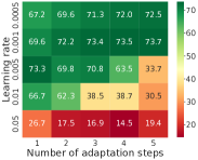
(a) TENT

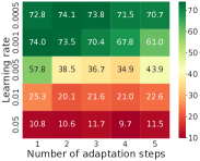
(b) SHOT

Figure 2: On the hyperparameter sensitivity of TTA methods, for evaluating the adaptation performance (test accuracy) of TENT and SHOT on CIFAR10-C (gaussian noise), under the combinations of learning rate and # of adaptation steps. The results indicate that the commonly used practice of selecting hyperparameters, e.g. setting the number of adaptation steps to $1$ while slightly varying the learning rate, does not necessarily lead to an improvement in test accuracy (it may even have detrimental effects). This phenomenon occurs in all corruption types.

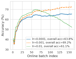
(a) Batch dependency exists in the online TTA setting with a single adaptation step.

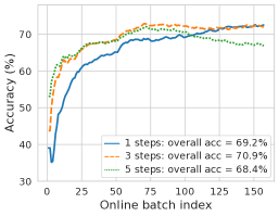
(b) Multiple-step improves TTA but still has strong dependency among batches.

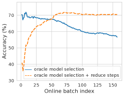
(c) Oracle model selection may introduce a more serious dependency problem to TTA.

Figure 3: The batch dependency issue during TTA and non-trivial model selection, for evaluating SHOT on CIFAR10-C (gaussian noise). Similar trends can be found in all corruption types. SHOT suffers a significant decline in performance in an online adaptation setting, particularly when improper hyperparameters are chosen. Despite efforts to improve adaptation performance through the implementation of multiple adaptation steps, the problem of batch dependency remains unresolved. Oracle model selection, while providing reliable label information to guide the adaptation process at test time, ultimately leads to even more severe dependency issues.

Batch Dependency.

Given that most existing TTA methods tend to leverage distribution knowledge (i.e. adaptation history) learned from previous test batches to improve the test-time performance on new samples, we further examine the influence of hyperparameter choices on adaptation dynamics. Figure 3(a) shows the common online setting with a single adaptation step and a range of learning rates, where we observe clear over-adaptation as TTA progresses with a large learning rate. Moving to the phase of multiple adaptation steps with a relatively small learning rate in Figure 3(b), we observe that adaptation performance increases from 69.2% to 70.9%. However, if we continue to increase the number of adaptation steps, the adaptation performance quickly drops to 68.4% due to over-adaptation on previous test batches. The risk of over-adaptation raises a practical question: when should we terminate TTA given a stream of test examples? We next examine the challenge of model selection in the online TTA setting.

4.2 Difficulty of TTA Model Selection

Model selection has recently gained great attention in the field of Domain Generalization (Gulrajani & Lopez-Paz, 2021) and Domain Adaptation (You et al., 2019). Yet, its importance and necessity in the context of TTA have been largely unexplored. We seek to shed light on this by exploring model selection in two paradigms: (i) with oracle information and (ii) with auxiliary regularization.

Oracle Information.

We first consider an oracle setting, where we assume access to true labels and select the optimal model (with early stopping) for each test batch with a sufficient number of adaptation steps. This approach is expected to achieve the highest possible adaptation performance per adaptation batch. For the sake of simplicity, we select the method-specific hyperparameters of each TTA method following the prior work (see more details in section C.1), while focusing on tuning two key adaptation-specific hyperparameters, namely learning rate and number of adaptation steps, which are highly relevant to the adaptation process detailed in section 3.2. We choose the maximum steps in Algorithm 1 as 50 according to our observation in Figure 2 and set the maximum steps as 25 in large-scale datasets due to the computational feasibility. The implementation is detailed in Algorithm 1.

Figure 3(c) shows that utilizing an oracle model selection strategy in TTA methods under an online adaptation setup with sufficient adaptation steps initially improves adaptation performance in the first several test batches, compared to Figure 3(a) and 3(b). However, such improvement is short-lived, as the adaptation performance quickly drops in subsequent test batches. It suggests that the oracle model selection strategy exacerbates the batch dependency problem when considering its use in isolation. This phenomenon is consistent across various choices of learning rates. Additionally, we find the same problem in TENT and NOTE as shown in Figure 10 of section B.2.

Auxiliary Regularization.

Given the suboptimality of the oracle-based model selection, we further investigate the effect of auxiliary regularization on mitigating batch dependency. Specifically, we consider Fisher regularizer (Niu et al., 2022b) and stochastically restoring (Wang et al., 2022), two regularizers originally proposed for non-stationary distribution shifts. Our results in Figure 8 of section B.1 indicate that while these strategies may alleviate the negative effects of batch dependence to some extent, there is currently no principle to trade-off the adaptation and regularization within a test batch, and leave the challenge of balancing adaptation across batches touched. These techniques are infeasible to consider in model selection and cannot provide a fair assessment for TTA methods, due to the increased sensitivity to their hyperparameters; see a significant variance caused by the regularization method across different learning rates and adaptation steps in Figure 9 of section B.1.

Algorithm 1 Oracle model selection for online TTA

Input: model state $\bm{\theta}^{o}$, test sample $\mathbf{x}^{(t)}$, true label $y^{(t)}$, maximum adaptation steps $M$, learning rate $\eta$, objective function $\ell$, update rule $\mathcal{G}$, and model selection metric $\mathcal{J}$. Oracle_model_selection$\bm{\theta},\ldots$Initialize: $m\leftarrow 1,\mathcal{F}\leftarrow\{\bm{\theta}\},\bm{\theta}_{m}\leftarrow\bm{\theta}$$m\in\{1,\cdots,M\}$Compute loss $\tilde{\ell}\approx\ell(\bm{\theta}_{m};x^{(t)})$Adapt parameters via $\bm{\theta}_{m+1}\leftarrow\mathcal{G}(\bm{\theta}_{m},\eta,\tilde{\ell})$$\mathcal{F}\leftarrow\mathcal{F}\cup\bm{\theta}_{m+1}$Select optimal model $\bm{\theta}^{\star}\!\leftarrow\!\operatorname*{arg\,max}_{\tilde{\bm{\theta}}\in\mathcal{F}}\mathcal{J}(\tilde{\bm{\theta}},y^{(t)})$Pass $\bm{\theta}^{\star}$to next test sample $\mathbf{x}^{(t+1)}$

4.3 Evaluation with Oracle Model Selection

In light of the aforementioned model selection difficulty, we design two evaluation protocols for estimating the potential of a given TTA method. The first one resorts to episodic adaptation with oracle model selection. It fully eliminates the impact of batch dependency, resulting in stable TTA outcomes. However, the performance gain of this protocol is often limited as it discards the valuable information from the previous batch about test data distribution.

As an alternative, the use of online adaptation empowers a large potential by accumulating historical knowledge. However, it presents a batch dependency challenge, posing model selection during TTA as a min-max equilibrium optimization problem across time and potentially leading to a significant decline in performance. To mitigate this issue, we use oracle model selection in conjecture with grid search over the best combinations of learning rates and adaptation steps. While such a traverse is computationally expensive, it allows for a reliable estimate of the optimal performance of each TTA method.

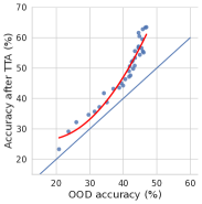
(a) OOD v.s. OOD (BN_Adapt).

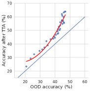
(b) OOD v.s. OOD (TENT).

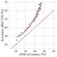
(c) OOD v.s. OOD (SHOT).

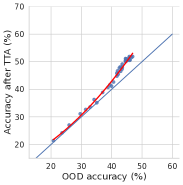
(d) OOD v.s. OOD (T3A).

Figure 4: The impact of model quality on TTA performance, in terms of OOD v.s. OOD (TTA) on CIFAR10-C. We save the checkpoints from the pre-training phase of ResNet-26 with standard augmentation and evaluate TTA performance on these checkpoints using oracle model selection. The OOD generalization performance has a significant impact on the overall performance (i.e. averaged accuracy of all corruption types) of various TTA methods. Our analysis reveals a strong correlation between model quality and the effectiveness of TTA methods. Furthermore, certain TTA methods, specifically SHOT, may not provide an improvement in performance on OOD datasets and may even result in a decrease in performance when applied to models of low quality.

5 Pre-trained Model Bottlenecks TTA Efficacy

Recall that several recent TTA methods outlined in Table 1 necessitate modifications of pre-training, which naturally results in inconsistent model qualities across methods and may deteriorate the test performance even before the TTA. In this section, we conduct a comprehensive and large-scale evaluation to examine the impact of base model quality on TTA performance across various TTA methods.

Evaluation setups.

We thoroughly examine the pre-trained model quality from the aspects of (1) disentangled feature extractor and classifier, and (2) data augmentation.

1. We consider a model with decoupled feature extractor and classifier. We keep the checkpoints with varying performance levels, generated from the pre-training phase using the standard data augmentation technique (mentioned below). We then fine-tune a trainable linear classifier for each frozen feature extractor from the checkpoints, using data with a uniform label distribution, to study the effect of the feature extractors (equivalently full model). To study the effect of the linear classifiers, we freeze a well-trained feature extractor and fine-tune trainable linear classifiers on several non-i.i.d. datasets created from a Dirichlet distribution; we further use Dirichlet distribution to create non-i.i.d. test data streams.

2. We consider 5 data augmentation policies: (i) no augmentations, (ii) standard augmentation, i.e. random crops and horizontal flips, (iii) MixUp (Zhang et al., 2017) combined with standard augmentations, (iv) AugMix (Hendrycks et al., 2019), and (v) PixMix (Hendrycks et al., 2022). For each data augmentation method, we save the checkpoints from the standard supervised pre-training phase to cover a wide range of pre-trained model qualities.

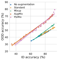
(a) ID v.s. OOD

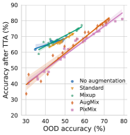
(b) OOD v.s. OOD (BN_Adapt)

(c) OOD v.s. OOD (TENT)

(d) OOD v.s. OOD (SHOT)

Figure 5: The impact of data augmentation policy on the TTA performance of the target domain. We save various sequences of checkpoints from the pre-training phase of ResNet-26 with five data augmentation policies and fine-tune each sequence to study the impact of data augmentation. TENT and SHOT use episodic adaptation with oracle model selection. Different data augmentation strategies have different corruption robustness, which causes varying generalization performance on CIFAR10-C. However, good practice in data augmentations and architecture designs for out-of-distribution generalization can be bad for test-time adaptation.

(a) domain #0

(b) domain #1

(c) domain #2

(d) domain #3

	domain #0 (%) $\downarrow$	domain #1 (%) $\downarrow$	domain #2 (%) $\downarrow$	domain #3 (%) $\downarrow$
Baseline	$12.6$	$96.5$	$79.9$	$76.1$
BN_Adapt	$7.9$	$98.4$	$85.8$	$80.7$
T3A	$22.0$	$96.0$	$77.5$	$74.8$
TENT	$7.0$	$98.1$	$84.4$	$80.1$
SHOT	$\mathbf{5.4}$	$\mathbf{95.0}$	$\mathbf{72.1}$	$\mathbf{67.4}$
TTT	$6.3$	$96.7$	$77.0$	$73.5$
MEMO	$10.1$	$97.4$	$83.7$	$80.3$

Figure 6: Adaptation performance (error) of TTA methods over CIFAR10-C with different label shifts. (a) test domain #0: $\alpha=0.1$, same label distribution with training environment. (b) test domain #1: $\alpha=0.1$, different label distribution with training environment. (c) test domain #2: $\alpha=1$. (d) test domain #3: uniformly distributed test stream. We investigate the impact of the degree of non-i.i.d.-ness in the fine-tuning dataset on the performance of the linear classifier. Label smoothing (Liang et al., 2020) technique is used to learn higher quality features. Our findings reveal that the quality of the linear classifier plays a crucial role in determining the effectiveness of TTA methods, as they can only enhance performance on test data that shares similar i.i.d.-ness and label distribution characteristics. Despite utilizing a well-trained feature extractor, the quality of the linear classifier remains a significant determining factor in the overall performance of TTA methods.

On the influence of the feature extractor (equivalently full model).

The results of our study, as depicted in Figure 4, reveal a strong correlation between the performance of test-time augmentation and out-of-distribution generalization on CIFAR10-C. Our analysis shows that across a wide range of TTA methods, the OOD generalization performance is highly indicative of TTA performance. A quadratic regression line was found to be an appropriate fit for the data, suggesting that TTA methods are more effective when applied to models of higher (OOD) quality.

On the influence of the linear classifier.

Our study has revealed that the performance of TTA methods is significantly impacted by the quality of the feature extractor used. The question then arises, can TTA methods bridge the distribution shift gap when equipped with a high-quality feature extractor and a suboptimal linear classifier? Our analysis, as shown in Figure 6(a)-LABEL:sub@fig:test_env2, indicates that most TTA methods on CIFAR10-C are only able to mitigate the distribution shift gap when the label distribution of the target domain is identical to that of the source domain, at which point the classifier is considered optimal. In this case, SHOT attains a 5.4% error rate, the best result observed in test domain #0. However, it is clear that all TTA methods either perform worse than the baseline in the remaining $3$ test domains or yield only marginal improvements over the baseline. These findings suggest that the quality of the classifier plays a crucial role in determining the performance of TTA methods.

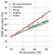
(a) ID v.s. OOD

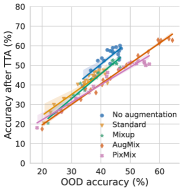
(b) OOD v.s. OOD (SHOT)

Figure 7: Revisit the impact of data augmentation policy on the TTA performance by using CCT. With the same data augmentation policies as in Figure 5, we save 5 sequences of checkpoints with different model quality and investigate the performance of SHOT under oracle model selection on CCT, a computationally efficient variant of ViT. The same trend as in ResNet-26 and WideResNet40-2 can be observed from CCT, emphasizing the unfavorable impact of strong data augmentation strategies on TTA performance regardless of the architecture designs.

On the influence of the data augmentation strategies.

We investigate the impact of various augmentation policies on the performance of ResNet-26 models trained on the CIFAR10 dataset. Our experimental results, as depicted in Figure 5 (more results in Figure 11 of section E.1), reveal that models pre-trained with the augmentation techniques like AugMix and PixMix exhibit superior OOD generalization performance on CIFAR10-C compared to models that do not utilize augmentation or only employ standard augmentations. Interestingly, even though these robust augmentation strategies significantly improve the robustness of the base model in the target domain, they only result in a marginal performance increase when combined with TTA. This disparity is particularly pronounced when compared to the performance of models trained with no augmentation or standard augmentations. However, when all models are fully trained in the source domain, the use of techniques such as AugMix and PixMix still leads to the best adaptation performance on CIFAR10-C, owing to their exceptional OOD generalization capabilities. We reach the same conclusion across both evaluation protocols and different architectures (e.g., WideResNet40-2) as shown in section E.1. In order to prove the influence of data augmentation strategies on TTA performance, we also conduct experiments on CCT, a computationally efficient variant of ViT and present experimental results in Figure 7. We highlight that good practice in strengthening the generalization performance of the base model in the target domain will decline its ability to bridge the distribution gap in the test time regardless of architecture designs.

6 No TTA Methods Mitigate All Shifts Yet

Table 2: Adaptation performance (error) of TTA methods over OOD datasets with common distribution shifts. Optimal results in episodic & online are highlighted by bold and blue respectively.

	CIFAR10-C (%) $\downarrow$	CIFAR100-C (%) $\downarrow$	ImageNet-C (%) $\downarrow$	CIFAR10.1 (%) $\downarrow$	OfficeHome (%) $\downarrow$	PACS (%) $\downarrow$
Baseline	$44.3$	$68.7$	$82.4$	$12.8$	$39.2$	$39.5$
BN_Adapt	$27.5\pm 0.1$	$56.5\pm 0.1$	$72.3\pm 0.1$	$19.0\pm 0.4$	$39.6\pm 0.1$	$27.6\pm 0.1$
SHOT-episodic	$21.6\pm 0.0$	$49.2\pm 0.1$	$68.0\pm 0.0$	$11.8\pm 0.2$	$35.9\pm 0.0$	$\mathbf{22.0\pm 0.1}$
SHOT-online	$21.0\pm 0.1$	$46.8\pm 0.1$	$62.4\pm 0.0$	$14.8\pm 0.0$	$35.5\pm 0.1$	$17.8\pm 0.1$
TTT-episodic	$\mathbf{20.9\pm 0.4}$	$51.8\pm 0.2$	-	$12.5\pm 0.1$	$40.2\pm 0.0$	$25.3\pm 0.1$
TTT-online	$20.0\pm 0.1$	$51.9\pm 0.1$	-	$13.5\pm 0.0$	$42.2\pm 0.1$	$26.6\pm 0.1$
TENT-episodic	$26.9\pm 0.0$	$54.6\pm 0.1$	$70.3\pm 0.0$	$18.6\pm 0.4$	$38.4\pm 0.0$	$26.1\pm 0.1$
TENT-online	$21.7\pm 0.1$	$49.9\pm 0.2$	$61.9\pm 0.1$	$17.9\pm 0.2$	$37.6\pm 0.0$	$22.7\pm 0.2$
T3A	$40.3\pm 0.1$	$67.6\pm 0.0$	$83.1\pm 0.0$	$12.5\pm 0.1$	$\mathbf{35.7\pm 0.1}$	$31.0\pm 0.4$
CoTTA-episodic	$25.3\pm 0.1$	$55.3\pm 0.1$	$94.0\pm 0.0$	$19.1\pm 0.4$	$53.7\pm 0.0$	$28.6\pm 0.1$
CoTTA-online	$42.5\pm 0.1$	$78.1\pm 0.1$	$94.4\pm 0.1$	$39.4\pm 1.2$	$52.9\pm 0.3$	$31.7\pm 0.2$
MEMO-episodic	$38.1\pm 0.1$	$65.3\pm 0.0$	$81.3\pm 0.0$	$\mathbf{10.8\pm 0.1}$	$37.6\pm 0.0$	$39.4\pm 0.0$
MEMO-online	$85.2\pm 0.7$	$96.3\pm 0.2$	$99.4\pm 0.1$	$14.2\pm 1.1$	$91.3\pm 0.1$	$75.5\pm 0.4$
NOTE-episodic	$32.4\pm 0.0$	$60.0\pm 0.0$	$80.8\pm 0.3$	$12.0\pm 0.1$	$37.9\pm 0.0$	$32.0\pm 0.1$
NOTE-online	$24.0\pm 0.1$	$54.5\pm 0.2$	$69.8\pm 0.1$	$12.7\pm 0.2$	$37.9\pm 0.1$	$27.7\pm 0.0$
Conjugate PL-episodic	$26.9\pm 0.0$	$54.4\pm 0.1$	$70.0\pm 0.1$	$18.7\pm 0.3$	$38.0\pm 0.1$	$25.3\pm 0.1$
Conjugate PL-online	$22.9\pm 0.1$	$51.0\pm 0.3$	$62.2\pm 0.0$	$18.3\pm 0.2$	$37.5\pm 0.1$	$21.8\pm 0.1$
SAR-episodic	$24.5\pm 0.0$	$54.6\pm 0.1$	$70.6\pm 0.1$	$17.1\pm 0.2$	$38.1\pm 0.0$	$26.2\pm 0.1$
SAR-online	$21.9\pm 0.1$	$49.7\pm 0.1$	$59.1\pm 0.3$	$18.0\pm 0.1$	$37.9\pm 0.0$	$22.7\pm 0.2$

The efficacy of TTA is contingent upon the nature of distributional variations. Specifically, the advantages demonstrated in previous research in the context of uncorrelated attribute shifts cannot be extrapolated to other forms of distributional shifts, such as shifts in spurious correlation, label shifts, and non-stationary shifts. In this section, we employ two evaluation protocols previously outlined in section 4.3 to re-evaluate commonly used datasets for distributional shifts, as well as benchmarks for distributional shifts that have been infrequently or never evaluated by prevalent TTA methods. Table 2 and Table 3 summarize the results of our experiments on all benchmarks for distributional shifts. Details of evaluation setups can be found in section C.1.

Common distribution shifts.

Here our evaluation of TTA performance primarily focuses on three areas: synthetic co-variate shift (i.e. CIFAR10-C), natural shift (i.e. CIFAR10.1), and domain generalization (i.e. OfficeHome and PACS). Except for online MEMO, all methods improve average performance across four common distributional shifts, although the extent of the adaptation performance gain varies among different TTA methods. Notably, online MEMO resulted in a significant degradation in adaptation performance, with an average test error of 66.6%, compared to 31.5% for episodic MEMO and 34.0% for the baseline, indicating that MEMO is only effective in episodic adaptation settings. Additionally, BN_Adapt, TENT, and TTT were unable to ensure improvement in adaptation performance on more challenging and realistic distributional shift benchmarks, such as CIFAR10.1 and OfficeHome. It should be noted that no single method consistently outperforms the others across all datasets under our fair evaluation. Niu et al. (2023) shows that batch normalization hinders stable TTA by estimating problematic mean and variance statistics, and prefers to use batch-agnostic norm layers, such as group norm (Wu & He, 2018) and layer norm (Ba et al., 2016). We provide additional benchmark results on architecture designs that utilize the group norm and layer norm in section F.2.

Table 3: Adaptation error (in %) of TTA methods over OOD datasets with two realistic distribution shifts. Dirichlet distribution is used to create non-i.i.d. test streams; the smaller value of $\alpha$ is, the more severe the label shift will be. Optimal results in episodic & online are highlighted by bold and blue respectively.

	Spurious correlation shifts $\downarrow$		Label shifts on CIFAR10 $\downarrow$
	ColoredMNIST	Waterbirds	$\alpha\!=\!0.01$	$\alpha\!=\!0.1$	$\alpha\!=\!1$
Baseline	$85.6$	$29.1$	$7.8\pm 2.3$	$5.5\pm 1.3$	$6.5\pm 0.8$
BN_adapt	$83.9\pm 0.2$	$38.1\pm 1.0$	$77.8\pm 1.7$	$64.5\pm 7.7$	$18.2\pm 1.0$
SHOT-episodic	$83.0\pm 0.3$	$29.4\pm 0.3$	$10.1\pm 2.5$	$7.3\pm 1.0$	$6.6\pm 0.8$
SHOT-online	$89.7\pm 0.2$	$27.0\pm 0.7$	$39.1\pm 3.1$	$30.0\pm 3.3$	$10.7\pm 1.0$
TTT-episodic	$78.1\pm 0.1$	$28.2\pm 0.3$	$11.0\pm 3.0$	$5.8\pm 1.7$	$6.6\pm 1.6$
TTT-online	$67.1\pm 1.3$	$24.0\pm 1.9$	$9.0\pm 2.3$	$6.1\pm 1.3$	$7.2\pm 1.4$
TENT-episodic	$83.9\pm 0.2$	$37.7\pm 1.0$	$76.8\pm 1.9$	$63.3\pm 7.1$	$17.6\pm 0.8$
TENT-online	$84.3\pm 0.2$	$24.2\pm 0.4$	$76.3\pm 2.1$	$62.2\pm 6.5$	$16.2\pm 0.4$
T3A	$88.1\pm 0.1$	$\mathbf{22.3\pm 0.2}$	$15.9\pm 3.5$	$9.6\pm 0.7$	$7.2\pm 0.6$
CoTTA-episodic	$\mathbf{72.6\pm 0.2}$	$31.7\pm 0.4$	$74.7\pm 1.7$	$61.1\pm 7.4$	$17.0\pm 1.2$
CoTTA-online	$87.0\pm 0.5$	$25.5\pm 1.5$	$80.5\pm 2.0$	$70.6\pm 5.0$	$31.7\pm 5.3$
MEMO-episodic	$84.9\pm 0.1$	$34.3\pm 0.1$	$\mathbf{0.1\pm 0.0}$	$\mathbf{1.2\pm 0.9}$	$\mathbf{4.5\pm 0.6}$
NOTE-episodic	$83.5\pm 0.1$	$30.0\pm 0.4$	$7.9\pm 2.3$	$5.4\pm 1.1$	$5.7\pm 0.7$
NOTE-online	$83.4\pm 0.4$	$43.3\pm 6.3$	$9.0\pm 2.1$	$6.2\pm 1.1$	$6.4\pm 0.7$
Conjugate PL-episodic	$83.9\pm 0.2$	$37.9\pm 0.9$	$76.9\pm 1.9$	$63.8\pm 7.4$	$17.6\pm 0.8$
Conjugate PL-online	$87.3\pm 0.3$	$23.7\pm 2.9$	$72.2\pm 0.3$	$59.5\pm 7.0$	$16.0\pm 0.1$
SAR-episodic	$83.9\pm 0.2$	$37.4\pm 1.1$	$75.3\pm 1.5$	$62.0\pm 7.7$	$15.5\pm 1.0$
SAR-online	$83.9\pm 0.2$	$34.6\pm 0.5$	$75.8\pm 1.4$	$61.1\pm 6.7$	$16.0\pm 0.6$

Spurious correlation shifts.

To the best of our knowledge, this study represents the first examination of the efficacy of dominant TTA methods in addressing spurious correlation shifts as demonstrated in the ColoredMNIST and Waterbirds benchmarks. As shown in Table 3, while some TTA methods demonstrate a reduction in error rate compared to the baseline, none of TTA methods can improve performance on the ColoredMNIST benchmark, as even a randomly initialized model exhibits a 50% error rate on this dataset. In terms of addressing the spurious correlation shift in the Waterbirds dataset, only T3A and TTT can consistently improve adaptation performance, as measured by worst-group error. TENT and SHOT may potentially improve performance on Waterbirds, but only through the utilization of impractical model selection techniques. The adaptation results presented in appendix F, are obtained through the use of commonly accepted practices in terms of hyperparameter choices, and adhere to the evaluation protocol established in previous research.

Label shifts.

Boudiaf et al. (2022) and Gong et al. (2022a) have taken label shift into account in their research, but they paired it with co-variate shift on CIFAR10-C. In contrast, our work solely examines the effectiveness of various TTA methods in addressing label shifts on the CIFAR10 dataset. The experimental results indicate that all TTA methods, except the MEMO method, demonstrate a higher test error than the baseline under strong label shift conditions. Specifically, TTA methods that heavily rely on the test batch for recalculating Batch Normalization statistics, such as TENT and BN_Adapt, experience the most significant performance degradation, with BN_Adapt incurring a 77.8% test error and TENT experiencing over 76.0% error rate when the label shift parameter $\alpha$ is set to $0.01$.

Table 4: Adaptation performance (error in %) of TTA methods on continual distribution shifts. To make a fair comparison, we employ Batch Normalization (BN) layer and use the same checkpoint with the other methods in NOTE-episodic and NOTE-online. We reproduce the original implementation (with Instand-aware BN) and pretrain another base model in NOTE-online $\star$.

	Cont. dist. shifts
	CIFAR10-C	ImageNet-C
Baseline	$44.3$	$82.4$
BN_adapt	$79.9\pm 0.5$	$96.3\pm 0.7$
SHOT-episodic	$41.3\pm 0.1$	$80.8\pm 0.1$
SHOT-online	$51.2\pm 2.0$	$93.5\pm 2.1$
TTT-episodic	$27.8\pm 0.1$	-
TTT-online	$29.7\pm 0.9$	-
TENT-episodic	$79.2\pm 0.4$	$95.5\pm 0.6$
TENT-online	$79.6\pm 0.4$	$97.5\pm 0.6$
T3A	$43.2\pm 0.3$	$82.2\pm 1.1$
CoTTA-episodic	$76.0\pm 0.4$	$97.8\pm 0.6$
CoTTA-online	$82.6\pm 0.3$	$98.5\pm 0.8$
MEMO-episodic	$\mathbf{12.7}\pm 0.1$	$\mathbf{70.7}\pm 0.5$
NOTE-episodic	$39.2\pm 0.1$	$81.8\pm 0.5$
NOTE-online	$25.7\pm 0.1$	$72.2\pm 1.3$
Conjugate PL-episodic	$79.3\pm 0.4$	$95.4\pm 0.6$
Conjugate PL-online	$79.6\pm 0.4$	$98.5\pm 0.5$
SAR-episodic	$77.2\pm 0.5$	$95.4\pm 0.6$
SAR-online	$79.6\pm 0.4$	$97.2\pm 0.4$
NOTE-online $\star$	$21.8\pm 0.0$	-

Non-stationary shifts.

In Table 4 we report the adaptation performance of TTA methods on the temporally correlated CIFAR10-C dataset introduced in Gong et al. (2022a). Additionally, we reproduce NOTE in TTAB, which is the current SOTA in the benchmark of temporal correlated shifts. Our results indicate that, even with the appropriate model selection, TENT and BN_Adapt still fail to improve adaptation performance in the presence of non-stationary shifts. However, TTA methods (e.g., TTT and MEMO) demonstrate substantial performance gains when adapting to the temporally correlated test stream, likely due to their instance-aware adaptation strategies, which focus on individual test samples. Surprisingly, MEMO outperforms NOTE in our implementation, which demonstrates the necessity of proper model selection in the field.

7 Conclusion

We have presented TTAB, a large-scale open-sourced benchmark for test-time adaptation. Through thorough and systematic studies, we showed that current TTA methods fall short in three aspects critical for practical applications, namely the difficulty in selecting appropriate hyper-parameters due to batch dependency, significant variability in performance sensitive to the quality of the pre-trained model, and poor efficacy in the face of certain classes of distribution shifts. We hope the proposed benchmark will stimulate more rigorous and measurable progress in future test-time adaptation research.

Appendix A Messages

We summarize some key messages of the manuscript here.

Appendix B The Limits of Evaluation for TTA Methods

B.1 Recent Regularization Techniques Proposed to Resist Batch Dependency Problem

• On the influence of batch dependency problem as shown in Figure 8

• Stochastic restoring model parameters and Fisher regularizer still show large variance when considering multiple adaptation steps as shown in Figure 9.

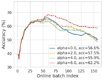
(a) Fisher regularizer

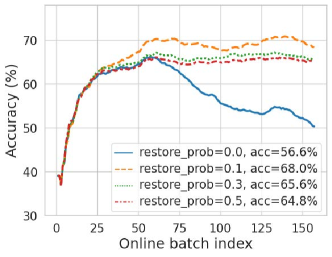
(b) Stochastic restoring

Figure 8: On the effect of fisher regularizer and stochastic restoring on batch dependency problem.

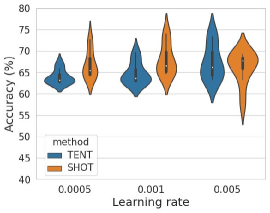
(a) Stochastic restoring: 1 steps

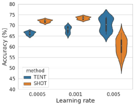
(b) Fisher regularizer: 1 steps

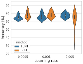
(c) Stochastic restoring: 2 steps

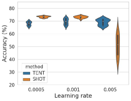
(d) Fisher regularizer: 2 steps

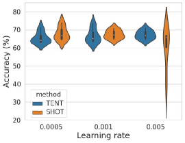
(e) Stochastic restoring: 3 steps

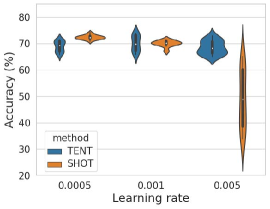
(f) Fisher regularizer: 3 steps

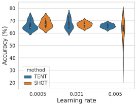
(g) Stochastic restoring: 4 steps

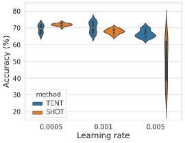
(h) Fisher regularizer: 4 steps

Figure 9: The standard deviation of stochastic restoring and Fisher regularizer when considering multiple adaptation steps. Fisher regularizer (Niu et al., 2022b) aims to constrain important model parameters from drastic changes to alleviate the error accumulated due to batch dependency. Stochastically restoring (Wang et al., 2022) involves a small portion of model parameters to their pre-trained values after adaptation on each test batch to prevent catastrophic forgetting. The hyperparameter tuning for these two techniques is challenging due to the high degree of variability inherent in these methods, which might impede their practical utility, particularly when compounded by the issue of batch dependency.

B.2 Optimal Model Selection for TTA is Non-trivial

Oracle model selection protocol also fails to solve the batch dependency issue in TENT and NOTE as shown in Figure 10

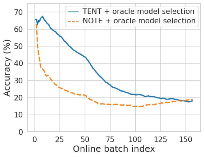
Figure 10: Oracle model selection also fails in TENT and NOTE under the online setting. Here we use ResNet-26 as the base model and learning rate is equal to 0.005.

Appendix C Implementation Details

C.1 Implementation Details of TTA Methods

Following prior work (Gulrajani & Lopez-Paz, 2021; Sun et al., 2020; Wang et al., 2022), we use ResNet-18/ResNet-26/ResNet-50 as the base model on ColoredMNIST/CIFAR10-C/large-scale image datasets and always choose SGDm as the optimizer. We choose method-specific hyperparameters following prior work. Following Iwasawa & Matsuo (2021), we assign the pseudo label in SHOT if the predictions are over a threshold which is 0.9 in our experiment and utilize $\beta=0.3$ for all experiments except $\beta=0.1$ for ColoredMNIST just as Liang et al. (2020). We set the number of augmentations $B=32$ for small-scale images (e.g. CIFAR10-C, CIFAR100-C) and $B=64$ for large-scale image sets like ImageNet-C, becasue this is the default option in Sun et al. (2020) and Zhang et al. . We simply set $N=0$ that controls the trade-off between source and estimated target statistics because it achieves performance comparable to the best performance when using a batch size of 64 according to Schneider et al. (2020). Training-domain validation data is used to determine the number of supports to store in T3A following Iwasawa & Matsuo (2021). We keep the average performance on the dataset if it has multiple test domains (e.g., CIFAR10-C, OfficeHome) and calculate the standard deviation over three different trials {2022, 2023, 2024}. We always examine the highest severity of corrupted data throughout our study.

C.2 Implementation Details of TTAB Methods

To establish a consistent and realistic evaluation framework for TTA methods, we have implemented several key choices. In contrast to the inconsistent pre-training strategies employed in previous studies, we have adopted a self-supervised learning approach utilizing the rotation prediction task as an auxiliary head, in conjunction with standard data augmentation techniques. This allows us to include TTT variants and maintain a consistent level of model quality across different TTA methods. For TTA methods that adapt a single image at a time (such as MEMO and TTT), we have modified the optimization procedure to accommodate larger batch sizes. Specifically, we have fixed the model parameters and accumulated gradients computed for each sample in a batch, only updating the model parameters once all samples have been adapted in a batch. Such a design excludes the unfairness caused by varied mini-batch sizes. We have utilized Stochastic Gradient Descent with momentum for TTA throughout all experiments conducted in this work (see the discrepancy in Table 1).

Appendix D Datasets

TTAB includes downloaders and loaders for all image classification tasks considered in our work:

• ColoredMNIST (Arjovsky et al., 2019) is a variant of the MNIST handwritten digit classification dataset. Domain $d\in\{0.1,0.3,0.9\}$ contains a disjoint set of digits colored either red or blue. The label is a noisy function of the digit and color, such that color bears correlation $d$ with the label and the digit bears correlation 0.75 with the label. This dataset contains 70000 examples of dimension $(2,28,28)$ and 2 classes.

• OfficeHome (Venkateswara et al., 2017) comprises four domains $d\in$ { art, clipart, product, real }. This dataset contains 15,588 examples of dimension $(3,224,224)$ and 65 classes.

• PACS (Li et al., 2017) comprises four domains $d\in$ { art, cartoons, photos, sketches }. This dataset contains 9,991 examples of dimension $(3,224,224)$ and 65 classes.

• CIFAR10 (Krizhevsky et al., 2009) consists of 60000 32x32 colour images in 10 classes, with 6000 images per class. There are 50000 training images and 10000 test images.

• CIFAR10-C (Hendrycks & Dietterich, 2019) is a dataset generated by adding 15 common corruptions + 4 extra corruptions to the test images in the Cifar10 dataset.

• CIFAR10.1 (Recht et al., 2018) contains roughly 2,000 new test images that were sampled after multiple years of research on the original CIFAR-10 dataset. The data collection for CIFAR-10.1 was designed to minimize distribution shift relative to the original dataset.

• Waterbirds (Sagawa et al., 2019) is constructed by cropping out birds from photos in the Caltech-UCSD Birds-200-2011 (CUB) dataset and transferring them onto backgrounds from the Places dataset.

Appendix E Model Quality

E.1 On the Influence of Data Augmentation

In Figure 11,  Figure 12, and Figure 13, we show more data augmentation results across different model architectures and different evaluation protocols.

(a) BN_Adapt

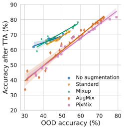
(b) TENT

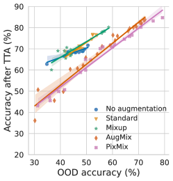
(c) SHOT

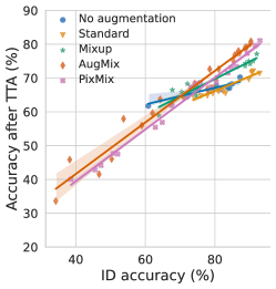
(d) BN_Adapt

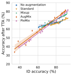
(e) TENT

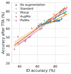
(f) SHOT

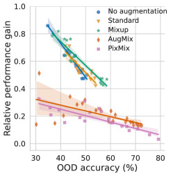
(g) BN_Adapt

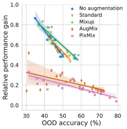
(h) TENT

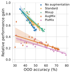
(i) SHOT

Figure 11: The effect of data augmentation on TTA performance in the target domain. TENT and SHOT use episodic adaptation with oracle model selection and choose ResNet-26 as the base model.

(a) BN_Adapt

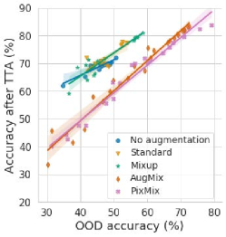
(b) TENT

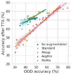
(c) SHOT

(d) BN_Adapt

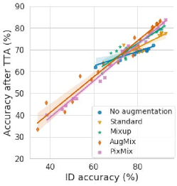
(e) TENT

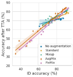
(f) SHOT

(g) BN_Adapt

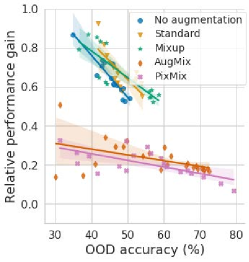
(h) TENT

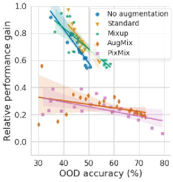
(i) SHOT

Figure 12: The effect of data augmentation on TTA performance in the target domain. TENT and SHOT use online adaptation without oracle model selection and grid search the best performance. We use ResNet-26 as the base model here.

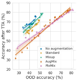
(a) BN_Adapt

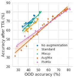
(b) TENT

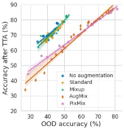
(c) SHOT

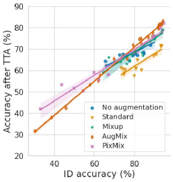
(d) BN_Adapt

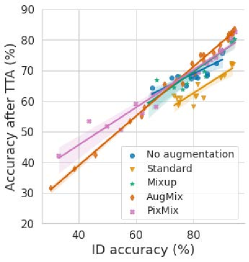
(e) TENT

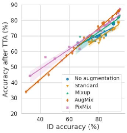
(f) SHOT

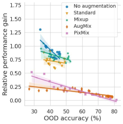
(g) BN_Adapt

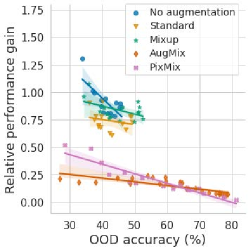
(h) TENT

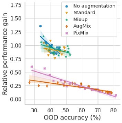
(i) SHOT

Figure 13: The effect of data augmentation on TTA performance in the target domain. TENT and SHOT use episodic adaptation with oracle model selection and choose WideResNet40-2 as the base model.

Appendix F Additional Results

F.1 TTA on Label Shifts

The efficacy of most TTA methods drops substantially when confronted with label shifts regardless of the data itself. Here we report the additional results of TTA methods on the CIFAR10-100 dataset, which is another common benchmark for evaluating distribution shift problems. The results are summarized in table 5.

Table 5: Adaptation performance (error in %) of TTA methods over label shifts on CIFAR100 with different severities. Optimal results are highlighted by bold.

	large label shift ($\alpha=1$) $\downarrow$		small label shift ($\alpha=10$) $\downarrow$
	episodic	online	episodic	online
Baseline	$31.2(\pm 1.2)$	$\mathbf{31.2(\pm 1.2)}$	$29.3(\pm 1.4)$	$29.3(\pm 1.4)$
BN_adapt	$41.9(\pm 1.3)$	$41.9(\pm 1.3)$	$37.7(\pm 2.0)$	$37.7(\pm 2.0)$
SHOT	$30.4(\pm 1.0)$	$32.6(\pm 1.8)$	$27.7(\pm 1.5)$	$29.5(\pm 1.7)$
TTT	$31.8(\pm 1.4)$	$32.9(\pm 1.5)$	$29.8(\pm 1.2)$	$31.2(\pm 1.4)$
TENT	$40.2(\pm 1.2)$	$38.8(\pm 1.1)$	$36.0(\pm 1.5)$	$35.4(\pm 1.9)$
T3A	$32.1(\pm 1.4)$	$32.1(\pm 1.4)$	$30.2(\pm 2.0)$	$30.2(\pm 2.0)$
CoTTA	$40.8(\pm 1.3)$	$68.4(\pm 0.7)$	$36.8(\pm 2.6)$	$67.0(\pm 1.5)$
MEMO	$\mathbf{28.3(\pm 1.3)}$	$32.1(\pm 2.6)$	$\mathbf{26.2(\pm 2.0)}$	$30.4(\pm 1.9)$
NOTE	$30.0(\pm 0.9)$	$\mathbf{31.2(\pm 1.1)}$	$28.2(\pm 1.7)$	$\mathbf{29.2(\pm 1.4)}$
Conjugate PL	$39.9(\pm 1.3)$	$37.9(\pm 1.9)$	$35.6(\pm 1.5)$	$36.1(\pm 2.1)$
SAR	$40.1(\pm 1.1)$	$39.0(\pm 1.1)$	$36.3(\pm 1.5)$	$35.8(\pm 1.5)$

F.2 Empirical Studies of Normalization Layers Effects in TTA

The most recent work (Niu et al., 2023) dug into the effects of normalization layers on TTA performance and found that TTA can perform more stably with batch-agnostic norm layers, i.e., group or layer norm. Here we revisit TTA performance on all data scenarios we have discussed before when equipped with group or layer norm.

Table 6: Results of TTA performance on ResNet26-GN. We report the error in (%) on CIFAR10-C severity level 5 under uniformly distributed test streams. Optimal results in episodic & online are highlighted by bold and blue respectively.

	Noise			Blur				Weather				Digital				Avg.
Model + Method	Gauss.	Shot	Impul.	Defoc.	Glass	Motion	Zoom	Snow	Frost	Fog	Brit.	Contr.	Elastic	Pixel	JPEG
ResNet26 (GN)	$56.1$	$51.6$	$51.5$	$21.6$	$42.4$	$20.5$	$25.1$	$20.6$	$24.7$	$19.7$	$11.6$	$13.6$	$25.6$	$48.6$	$30.6$	$30.9$
$\bullet~{}$SHOT-episodic	$40.8$	$38.6$	$45.7$	$19.9$	$40.0$	$19.1$	$23.3$	$19.9$	$23.1$	$18.8$	$11.1$	$13.0$	$24.2$	$38.8$	$29.2$	$27.0$
$\bullet~{}$SHOT-online	$29.9$	$27.5$	$35.4$	$14.1$	$34.0$	$14.6$	$15.1$	$18.2$	$18.9$	$16.0$	$10.4$	$11.7$	$22.3$	$20.0$	$24.6$	$20.8$
$\bullet~{}$TTT-episodic	$38.2$	$\mathbf{34.7}$	$\mathbf{40.6}$	$\mathbf{13.8}$	$\mathbf{37.4}$	$16.7$	$\mathbf{17.8}$	$18.4$	$\mathbf{19.6}$	$16.2$	$10.2$	$11.7$	$22.5$	$\mathbf{25.0}$	$24.8$	$\mathbf{23.2}$
$\bullet~{}$TTT-online	$27.9$	$24.5$	$32.6$	$13.5$	$35.7$	$16.3$	$16.9$	$18.8$	$17.5$	$14.8$	$10.6$	$11.5$	$23.3$	$18.0$	$22.0$	$20.2$
$\bullet~{}$TENT-episodic	$55.5$	$50.3$	$50.3$	$20.5$	$41.6$	$19.5$	$24.1$	$20.0$	$23.6$	$19.0$	$11.2$	$13.1$	$24.7$	$47.4$	$29.5$	$30.0$
$\bullet~{}$TENT-online	$86.4$	$80.9$	$82.1$	$14.7$	$49.8$	$15.1$	$16.4$	$19.7$	$20.9$	$16.7$	$10.5$	$12.5$	$24.3$	$70.6$	$30.6$	$36.8$
$\bullet~{}$T3A	$51.3$	$46.6$	$48.3$	$20.5$	$40.4$	$19.6$	$23.5$	$20.5$	$24.1$	$19.2$	$11.7$	$13.6$	$24.5$	$45.9$	$30.1$	$29.3$
$\bullet~{}$CoTTA-episodic	$\mathbf{38.0}$	$36.8$	$41.2$	$22.7$	$42.6$	$21.7$	$27.6$	$20.2$	$21.8$	$19.5$	$10.6$	$12.3$	$27.5$	$49.7$	$30.5$	$28.2$
$\bullet~{}$CoTTA-online	$55.3$	$57.3$	$50.1$	$47.5$	$73.6$	$44.2$	$54.2$	$37.8$	$41.9$	$44.0$	$12.9$	$15.2$	$62.7$	$67.7$	$56.4$	$48.1$
$\bullet~{}$MEMO-episodic	$55.7$	$50.3$	$49.7$	$15.8$	$39.0$	$\mathbf{15.0}$	$18.1$	$\mathbf{17.1}$	$19.7$	$\mathbf{15.3}$	$\mathbf{8.4}$	$\mathbf{11.2}$	$\mathbf{19.3}$	$45.5$	$\mathbf{22.9}$	$26.9$
$\bullet~{}$NOTE-episodic	$46.7$	$42.9$	$46.4$	$20.3$	$40.4$	$19.4$	$23.6$	$20.0$	$23.2$	$18.7$	$11.3$	$13.2$	$24.6$	$42.4$	$29.1$	$28.1$
$\bullet~{}$NOTE-online	$34.5$	$31.3$	$39.8$	$15.2$	$36.4$	$16.0$	$16.8$	$19.6$	$19.8$	$17.1$	$10.7$	$12.5$	$23.4$	$23.7$	$26.6$	$22.9$
$\bullet~{}$Conjugate PL-episodic	$55.6$	$50.6$	$50.5$	$20.6$	$41.7$	$19.7$	$24.2$	$20.1$	$23.8$	$19.2$	$11.3$	$13.2$	$24.7$	$47.7$	$29.6$	$30.2$
$\bullet~{}$Conjugate PL-online	$86.9$	$75.3$	$82.4$	$15.0$	$76.9$	$15.5$	$16.2$	$20.1$	$19.8$	$17.4$	$10.5$	$13.1$	$27.0$	$76.7$	$31.9$	$39.0$
$\bullet~{}$SAR-episodic	$51.6$	$47.7$	$48.0$	$19.6$	$39.8$	$18.3$	$22.6$	$18.6$	$22.5$	$17.7$	$10.7$	$12.5$	$22.9$	$46.0$	$28.3$	$28.4$
$\bullet~{}$SAR-online	$65.5$	$54.5$	$57.3$	$17.6$	$43.1$	$16.2$	$17.0$	$20.3$	$22.0$	$17.4$	$10.8$	$13.3$	$24.2$	$31.8$	$30.6$	$29.4$

Table 7: Results of TTA performance on ViTSmall (LN). We report the error in (%) on CIFAR10-C severity level 5 under uniformly distributed test streams. Optimal results in episodic & online are highlighted by bold and blue respectively.

	Noise			Blur				Weather				Digital				Avg.
Model + Method	Gauss.	Shot	Impul.	Defoc.	Glass	Motion	Zoom	Snow	Frost	Fog	Brit.	Contr.	Elastic	Pixel	JPEG
ViTSmall (LN)	$33.3$	$28.5$	$17.7$	$5.8$	$22.1$	$10.5$	$4.9$	$5.3$	$7.7$	$12.4$	$2.9$	$10.0$	$12.6$	$24.4$	$15.6$	$14.2$
$\bullet~{}$SHOT-episodic	$23.6$	$21.2$	$14.0$	$5.3$	$19.7$	$9.5$	$4.6$	$5.0$	$7.1$	$10.9$	$2.6$	$8.1$	$11.5$	$12.2$	$14.6$	$11.3$
$\bullet~{}$SHOT-online	$14.7$	$14.5$	$10.2$	$4.3$	$12.6$	$5.4$	$3.3$	$4.4$	$5.1$	$5.8$	$2.3$	$3.3$	$8.8$	$5.3$	$11.6$	$7.4$
$\bullet~{}$TTT-episodic	$\mathbf{14.4}$	$\mathbf{12.2}$	$\mathbf{8.7}$	$\mathbf{3.8}$	$\mathbf{13.6}$	$\mathbf{6.2}$	$\mathbf{3.0}$	$\mathbf{3.7}$	$\mathbf{4.8}$	$\mathbf{7.3}$	$2.1$	$\mathbf{4.2}$	$8.3$	$5.4$	$\mathbf{11.4}$	$\mathbf{7.3}$
$\bullet~{}$TTT-online	$10.8$	$9.5$	$6.6$	$3.9$	$10.3$	$5.3$	$3.2$	$3.8$	$4.0$	$4.8$	$2.2$	$2.8$	$7.8$	$4.3$	$10.0$	$5.9$
$\bullet~{}$TENT-episodic	$29.8$	$25.3$	$15.8$	$5.5$	$20.1$	$9.6$	$4.6$	$5.1$	$7.3$	$11.6$	$2.8$	$8.9$	$11.6$	$16.9$	$14.8$	$12.6$
$\bullet~{}$TENT-online	$18.7$	$16.9$	$10.5$	$4.3$	$12.8$	$6.6$	$3.4$	$4.6$	$5.3$	$5.8$	$2.4$	$3.5$	$8.9$	$5.8$	$12.1$	$8.1$
$\bullet~{}$T3A	$29.4$	$24.8$	$17.1$	$6.0$	$21.3$	$10.2$	$4.8$	$5.4$	$7.1$	$10.7$	$2.9$	$9.0$	$12.1$	$21.1$	$16.0$	$13.2$
$\bullet~{}$CoTTA-episodic	$81.7$	$82.2$	$75.5$	$4.8$	$76.0$	$22.9$	$3.8$	$4.0$	$6.4$	$32.3$	$\mathbf{1.9}$	$14.2$	$44.4$	$68.0$	$51.2$	$38.0$
$\bullet~{}$CoTTA-online	$88.6$	$88.8$	$87.6$	$5.3$	$87.4$	$39.9$	$4.0$	$4.6$	$5.3$	$48.9$	$2.7$	$11.7$	$67.6$	$82.8$	$78.4$	$46.9$
$\bullet~{}$MEMO-episodic	$20.9$	$17.5$	$13.2$	$4.1$	$15.2$	$6.9$	$3.4$	$3.9$	$5.3$	$8.0$	$\mathbf{1.9}$	$4.4$	$\mathbf{7.9}$	$\mathbf{4.9}$	$11.7$	$8.6$
$\bullet~{}$NOTE-episodic	$31.9$	$27.3$	$17.2$	$5.8$	$21.6$	$10.3$	$4.8$	$5.3$	$7.6$	$12.1$	$2.9$	$9.6$	$12.4$	$21.8$	$15.3$	$13.7$
$\bullet~{}$NOTE-online	$19.0$	$16.4$	$12.3$	$4.7$	$14.7$	$7.4$	$3.9$	$4.8$	$5.9$	$7.7$	$2.6$	$4.9$	$9.6$	$7.2$	$13.0$	$8.9$
$\bullet~{}$Conjugate PL-episodic	$30.1$	$24.9$	$15.5$	$5.5$	$20.0$	$9.4$	$4.6$	$5.1$	$7.3$	$11.5$	$2.8$	$8.7$	$11.7$	$15.4$	$14.8$	$12.5$
$\bullet~{}$Conjugate PL-online	$19.6$	$18.7$	$10.8$	$4.2$	$12.5$	$6.1$	$3.2$	$4.6$	$5.2$	$6.1$	$2.6$	$3.2$	$8.9$	$5.9$	$12.1$	$8.2$
$\bullet~{}$SAR-episodic	$29.2$	$24.8$	$15.5$	$5.7$	$19.6$	$9.4$	$4.8$	$5.3$	$7.6$	$11.2$	$2.9$	$8.6$	$11.6$	$17.5$	$14.3$	$12.5$
$\bullet~{}$SAR-online	$20.3$	$18.2$	$11.7$	$4.5$	$13.3$	$6.6$	$3.6$	$4.6$	$5.8$	$6.8$	$2.6$	$4.3$	$9.0$	$6.9$	$12.5$	$8.7$

Table 8: Results of TTA performance on ResNet50-GN. We report the error in (%) on ImageNet-C severity level 5 under uniformly distributed test streams. Optimal results in episodic & online are highlighted by bold and blue respectively.

	Noise			Blur				Weather				Digital				Avg.
Model + Method	Gauss.	Shot	Impul.	Defoc.	Glass	Motion	Zoom	Snow	Frost	Fog	Brit.	Contr.	Elastic	Pixel	JPEG
ResNet50 (GN)	$78.3$	$78.7$	$78.0$	$83.4$	$91.3$	$81.2$	$74.6$	$64.5$	$57.7$	$66.1$	$34.1$	$69.1$	$83.9$	$65.4$	$50.0$	$70.4$
$\bullet~{}$SHOT-episodic	$\mathbf{70.6}$	$\mathbf{69.5}$	$\mathbf{69.4}$	$82.3$	$\mathbf{84.9}$	$\mathbf{78.3}$	$\mathbf{72.1}$	$\mathbf{61.2}$	$57.7$	$\mathbf{58.9}$	$\mathbf{32.9}$	$\mathbf{66.2}$	$\mathbf{72.2}$	$\mathbf{56.7}$	$\mathbf{47.8}$	$\mathbf{65.4}$
$\bullet~{}$SHOT-online	$61.3$	$57.9$	$58.9$	$92.1$	$86.4$	$82.2$	$73.3$	$54.9$	$59.2$	$56.2$	$34.8$	$89.1$	$55.7$	$41.2$	$43.9$	$63.1$
$\bullet~{}$TENT-episodic	$77.6$	$78.0$	$77.2$	$82.8$	$91.0$	$80.9$	$74.3$	$64.2$	$\mathbf{57.3}$	$65.8$	$33.8$	$68.4$	$83.7$	$64.3$	$49.8$	$69.9$
$\bullet~{}$TENT-online	$86.6$	$78.9$	$83.5$	$90.5$	$98.5$	$88.5$	$80.1$	$83.3$	$81.6$	$83.4$	$33.2$	$63.9$	$96.2$	$54.7$	$49.9$	$76.8$
$\bullet~{}$T3A	$84.7$	$84.3$	$84.9$	$85.0$	$92.1$	$83.6$	$75.4$	$64.5$	$58.8$	$66.2$	$34.1$	$71.6$	$83.2$	$66.5$	$51.0$	$72.4$
$\bullet~{}$CoTTA-episodic	$91.9$	$92.5$	$90.9$	$93.7$	$97.2$	$89.8$	$83.9$	$73.7$	$66.0$	$72.0$	$47.5$	$82.3$	$90.7$	$83.2$	$61.9$	$81.2$
$\bullet~{}$CoTTA-online	$98.8$	$99.1$	$98.9$	$99.2$	$99.6$	$98.2$	$94.7$	$98.5$	$96.1$	$92.0$	$69.1$	$93.6$	$99.0$	$98.4$	$81.7$	$94.5$
$\bullet~{}$MEMO-episodic	$77.0$	$77.5$	$76.3$	$83.0$	$86.6$	$79.0$	$72.7$	$63.0$	$57.6$	$62.9$	$\mathbf{32.9}$	$67.8$	$82.1$	$58.1$	$48.1$	$68.3$
$\bullet~{}$NOTE-episodic	$78.3$	$78.7$	$78.0$	$83.4$	$91.3$	$81.2$	$74.6$	$64.5$	$57.7$	$66.0$	$34.0$	$69.1$	$83.9$	$65.4$	$50.0$	$70.4$
$\bullet~{}$NOTE-online	$77.3$	$77.0$	$76.6$	$83.3$	$90.5$	$80.3$	$74.0$	$64.2$	$57.7$	$64.8$	$33.9$	$67.7$	$82.8$	$62.5$	$49.7$	$69.5$
$\bullet~{}$Conjugate PL-episodic	$76.2$	$75.8$	$75.5$	$\mathbf{82.0}$	$90.4$	$79.9$	$73.0$	$63.4$	$\mathbf{57.3}$	$66.0$	$33.0$	$\mathbf{66.2}$	$82.9$	$60.3$	$48.6$	$68.7$
$\bullet~{}$Conjugate PL-online	$93.3$	$87.0$	$91.5$	$97.4$	$99.3$	$96.7$	$89.8$	$96.5$	$94.6$	$98.3$	$29.2$	$61.0$	$99.0$	$40.3$	$43.7$	$81.2$
$\bullet~{}$SAR-episodic	$77.1$	$77.3$	$76.6$	$82.4$	$90.6$	$80.3$	$73.9$	$64.0$	$57.4$	$65.1$	$33.6$	$67.8$	$83.4$	$63.4$	$49.7$	$69.5$
$\bullet~{}$SAR-online	$60.1$	$57.1$	$58.5$	$83.9$	$92.2$	$57.8$	$55.3$	$54.1$	$55.7$	$41.7$	$28.8$	$49.9$	$94.0$	$38.8$	$42.4$	$58.0$

Table 9: Results of TTA performance on ViTBase (LN). We report the error in (%) on ImageNet-C severity level 5 under uniformly distributed test streams. Optimal results in episodic & online are highlighted by bold and blue respectively.

	Noise			Blur				Weather				Digital				Avg.
Model + Method	Gauss.	Shot	Impul.	Defoc.	Glass	Motion	Zoom	Snow	Frost	Fog	Brit.	Contr.	Elastic	Pixel	JPEG
ViTBase (LN)	$74.1$	$78.2$	$75.4$	$70.1$	$78.6$	$67.5$	$73.1$	$84.2$	$75.3$	$52.8$	$46.4$	$56.8$	$70.3$	$52.1$	$48.8$	$66.9$
$\bullet~{}$SHOT-episodic	$\mathbf{56.7}$	$\mathbf{56.7}$	$\mathbf{56.0}$	$\mathbf{52.6}$	$\mathbf{59.7}$	$\mathbf{50.1}$	$\mathbf{52.4}$	$\mathbf{43.3}$	$\mathbf{45.3}$	$\mathbf{39.4}$	$26.3$	$\mathbf{41.6}$	$\mathbf{50.8}$	$35.0$	$39.9$	$\mathbf{47.0}$
$\bullet~{}$SHOT-online	$73.2$	$60.5$	$59.5$	$63.9$	$57.5$	$49.2$	$42.2$	$42.9$	$46.6$	$34.0$	$24.8$	$60.8$	$34.4$	$29.1$	$34.7$	$47.6$
$\bullet~{}$TENT-episodic	$73.4$	$77.3$	$74.7$	$69.0$	$78.0$	$66.7$	$72.3$	$83.4$	$74.2$	$52.1$	$45.1$	$55.8$	$69.7$	$51.1$	$48.3$	$66.1$
$\bullet~{}$TENT-online	$50.5$	$50.1$	$51.9$	$44.8$	$45.5$	$39.4$	$46.8$	$52.4$	$72.7$	$28.7$	$23.0$	$35.2$	$50.1$	$27.3$	$31.3$	$43.3$
$\bullet~{}$T3A	$74.7$	$78.9$	$75.8$	$70.5$	$78.9$	$67.6$	$72.7$	$84.6$	$75.5$	$51.8$	$46.0$	$57.4$	$68.8$	$52.6$	$48.8$	$67.0$
$\bullet~{}$CoTTA-episodic	$98.6$	$98.6$	$99.1$	$95.5$	$97.8$	$92.8$	$88.1$	$86.9$	$97.3$	$92.6$	$55.1$	$95.6$	$98.1$	$89.4$	$64.6$	$90.0$
$\bullet~{}$CoTTA-online	$99.4$	$99.5$	$99.5$	$99.6$	$99.7$	$99.4$	$99.3$	$99.2$	$99.3$	$99.3$	$96.3$	$99.5$	$99.5$	$99.0$	$92.5$	$98.7$
$\bullet~{}$MEMO-episodic	$68.8$	$74.3$	$70.4$	$60.1$	$66.6$	$55.7$	$57.0$	$54.3$	$58.4$	$45.4$	$\mathbf{23.9}$	$42.8$	$65.6$	$\mathbf{33.4}$	$\mathbf{36.9}$	$54.2$
$\bullet~{}$NOTE-episodic	$74.1$	$78.1$	$75.4$	$70.0$	$78.6$	$67.5$	$73.1$	$84.2$	$75.3$	$52.7$	$46.4$	$56.8$	$70.3$	$52.1$	$48.8$	$66.9$
$\bullet~{}$NOTE-online	$72.0$	$75.4$	$73.2$	$67.2$	$76.7$	$64.9$	$70.7$	$79.4$	$71.4$	$50.9$	$41.9$	$54.3$	$68.5$	$49.2$	$47.7$	$64.2$
$\bullet~{}$Conjugate PL-episodic	$69.1$	$72.8$	$70.2$	$65.1$	$74.3$	$63.3$	$68.7$	$80.7$	$71.7$	$48.7$	$41.4$	$50.4$	$67.3$	$46.4$	$45.7$	$62.4$
$\bullet~{}$Conjugate PL-online	$80.7$	$75.5$	$84.0$	$45.3$	$48.3$	$40.3$	$68.9$	$91.4$	$96.0$	$29.3$	$23.7$	$35.1$	$96.5$	$27.7$	$31.9$	$58.3$
$\bullet~{}$SAR-episodic	$73.6$	$77.6$	$75.0$	$69.4$	$78.3$	$67.1$	$72.7$	$83.6$	$74.7$	$52.4$	$45.8$	$56.3$	$70.0$	$51.7$	$48.6$	$66.5$
$\bullet~{}$SAR-online	$46.1$	$47.5$	$44.5$	$43.5$	$43.8$	$38.1$	$39.9$	$33.2$	$54.2$	$28.1$	$22.9$	$34.7$	$32.7$	$27.1$	$30.8$	$37.8$

Appendix G Additional Related Work

Unsupervised Domain Adaptation

Unsupervised Domain Adaptation (UDA) is a technique aimed at enhancing the performance of a target model in scenarios where there is a shift in distribution between the labeled source domain and the unlabeled target domain. UDA methods typically seek to align the feature distributions between the two domains through the utilization of discrepancy losses (Long et al., 2015) or adversarial training (Ganin & Lempitsky, 2015; Tsai et al., 2018).

Domain Generalization

Our work is also related to DG (Muandet et al., 2013; Blanchard et al., 2011) in a broad sense, due to the shared goal of bridging the gap of distribution shifts between the source domain and the target domain. Also, DG and TTA may share similar constraints on model selection for lacking label information in the target domain. DomainBed (Gulrajani & Lopez-Paz, 2021) highlights the necessity of considering model selection criterion in DG and concludes that ERM (Vapnik, 1998) outperforms the state-of-the-art in terms of average performance after carefully tuning using model selection criteria.

Distribution Shift Benchmarks.

Distribution shift has been widely studied in the machine learning community. Prior works have covered a wide range of distribution shifts. The first line of such benchmarks applies different transformations to object recognition datasets to induce distribution shifts. These benchmarks include: (1) CIFAR10-C & ImageNet-C (Hendrycks & Dietterich, 2019), ImageNet-A (Hendrycks et al., 2021b), ImageNet-R (Hendrycks et al., 2021a), ImageNet-V2 (Recht et al., 2019), and many others; (2) ColoredMNIST (Arjovsky et al., 2019), which makes the color of digits a confounder. Most recent benchmarks collect sets of images with various styles and backgrounds, such as PACS (Li et al., 2017), OfficeHome (Venkateswara et al., 2017), DomainNet (Peng et al., 2019), and Waterbirds (Sagawa et al., 2019). Unlike most prior works that assume a specific stationary target domain, the study on continuous TTA that considers continually changing target data becomes more and more popular in the field. Recently, a few works have constructed datasets and benchmarks for scenarios under temporal shifts. Gong et al. (2022b) builds a temporally correlated test stream on CIFAR10-C sample by a Dirichlet distribution, where most existing TTA methods fail dramatically. Wild-Time (Yao et al., 2022) benchmark consists of 5 datasets that reflect temporal distribution shifts arising in a variety of real-world applications, including patient prognosis and news classification. Studies on fairness and bias (Mehrabi et al., 2021) have investigated the detrimental impact of spurious correlation in classification (Geirhos et al., 2018) and conservation (Beery et al., 2020). To our knowledge, there have been rare TTA work focused on tackling spurious correlation shifts.

References

- Arjovsky et al. (2019) Arjovsky, M., Bottou, L., Gulrajani, I., and Lopez-Paz, D. Invariant risk minimization. arXiv preprint arXiv:1907.02893, 2019.
- Ba et al. (2016) Ba, J. L., Kiros, J. R., and Hinton, G. E. Layer normalization. arXiv preprint arXiv:1607.06450, 2016.
- Beery et al. (2020) Beery, S., Liu, Y., Morris, D., Piavis, J., Kapoor, A., Joshi, N., Meister, M., and Perona, P. Synthetic examples improve generalization for rare classes. In Proceedings of the IEEE/CVF Winter Conference on Applications of Computer Vision, pp. 863–873, 2020.
- Blanchard et al. (2011) Blanchard, G., Lee, G., and Scott, C. Generalizing from several related classification tasks to a new unlabeled sample. Advances in neural information processing systems, 24, 2011.
- Boudiaf et al. (2022) Boudiaf, M., Mueller, R., Ben Ayed, I., and Bertinetto, L. Parameter-free online test-time adaptation. In Proceedings of the IEEE/CVF Conference on Computer Vision and Pattern Recognition, pp. 8344–8353, 2022.
- Burns & Steinhardt (2021) Burns, C. and Steinhardt, J. Limitations of post-hoc feature alignment for robustness. In Proceedings of the IEEE/CVF Conference on Computer Vision and Pattern Recognition, pp. 2525–2533, 2021.
- Chen et al. (2022) Chen, D., Wang, D., Darrell, T., and Ebrahimi, S. Contrastive test-time adaptation. In Proceedings of the IEEE/CVF Conference on Computer Vision and Pattern Recognition, pp. 295–305, 2022.
- Eastwood et al. (2022) Eastwood, C., Mason, I., Williams, C., and Schölkopf, B. Source-free adaptation to measurement shift via bottom-up feature restoration. In International Conference on Learning Representations, 2022.
- Fleuret et al. (2021) Fleuret, F. et al. Uncertainty reduction for model adaptation in semantic segmentation. In Proceedings of the IEEE/CVF Conference on Computer Vision and Pattern Recognition, pp. 9613–9623, 2021.
- (10) Gandelsman, Y., Sun, Y., Chen, X., and Efros, A. A. Test-time training with masked autoencoders. In Advances in Neural Information Processing Systems.
- Ganin & Lempitsky (2015) Ganin, Y. and Lempitsky, V. Unsupervised domain adaptation by backpropagation. In International conference on machine learning, pp. 1180–1189. PMLR, 2015.
- Gao et al. (2022) Gao, J., Zhang, J., Liu, X., Darrell, T., Shelhamer, E., and Wang, D. Back to the source: Diffusion-driven test-time adaptation. arXiv preprint arXiv:2207.03442, 2022.
- Geirhos et al. (2018) Geirhos, R., Rubisch, P., Michaelis, C., Bethge, M., Wichmann, F. A., and Brendel, W. Imagenet-trained cnns are biased towards texture; increasing shape bias improves accuracy and robustness. arXiv preprint arXiv:1811.12231, 2018.
- Gong et al. (2022a) Gong, T., Jeong, J., Kim, T., Kim, Y., Shin, J., and Lee, S.-J. Note: Robust continual test-time adaptation against temporal correlation. In Advances in Neural Information Processing Systems (NeurIPS), 2022a.
- Gong et al. (2022b) Gong, T., Jeong, J., Kim, T., Kim, Y., Shin, J., and Lee, S.-J. Robust continual test-time adaptation: Instance-aware bn and prediction-balanced memory. arXiv preprint arXiv:2208.05117, 2022b.
- Goyal et al. (2022) Goyal, S., Sun, M., Raghunathan, A., and Kolter, Z. Test-time adaptation via conjugate pseudo-labels. In Advances in Neural Information Processing Systems (NeurIPS), 2022.
- Gulrajani & Lopez-Paz (2021) Gulrajani, I. and Lopez-Paz, D. In search of lost domain generalization. In International Conference on Learning Representations, 2021. URL https://openreview.net/forum?id=lQdXeXDoWtI.
- Hendrycks & Dietterich (2019) Hendrycks, D. and Dietterich, T. Benchmarking neural network robustness to common corruptions and perturbations. In International Conference on Learning Representations, 2019. URL https://openreview.net/forum?id=HJz6tiCqYm.
- Hendrycks et al. (2019) Hendrycks, D., Mu, N., Cubuk, E. D., Zoph, B., Gilmer, J., and Lakshminarayanan, B. Augmix: A simple data processing method to improve robustness and uncertainty. arXiv preprint arXiv:1912.02781, 2019.
- Hendrycks et al. (2021a) Hendrycks, D., Basart, S., Mu, N., Kadavath, S., Wang, F., Dorundo, E., Desai, R., Zhu, T., Parajuli, S., Guo, M., et al. The many faces of robustness: A critical analysis of out-of-distribution generalization. In Proceedings of the IEEE/CVF International Conference on Computer Vision, pp. 8340–8349, 2021a.
- Hendrycks et al. (2021b) Hendrycks, D., Zhao, K., Basart, S., Steinhardt, J., and Song, D. Natural adversarial examples. CVPR, 2021b.
- Hendrycks et al. (2022) Hendrycks, D., Zou, A., Mazeika, M., Tang, L., Li, B., Song, D., and Steinhardt, J. Pixmix: Dreamlike pictures comprehensively improve safety measures. CVPR, 2022.
- Iwasawa & Matsuo (2021) Iwasawa, Y. and Matsuo, Y. Test-time classifier adjustment module for model-agnostic domain generalization. Advances in Neural Information Processing Systems, 34:2427–2440, 2021.
- Jiang & Lin (2023) Jiang, L. and Lin, T. Test-time robust personalization for federated learning. In International Conference on Learning Representations, 2023.
- Koh et al. (2021) Koh, P. W., Sagawa, S., Marklund, H., Xie, S. M., Zhang, M., Balsubramani, A., Hu, W., Yasunaga, M., Phillips, R. L., Gao, I., et al. Wilds: A benchmark of in-the-wild distribution shifts. In International Conference on Machine Learning, pp. 5637–5664. PMLR, 2021.
- Krizhevsky et al. (2009) Krizhevsky, A., Hinton, G., et al. Learning multiple layers of features from tiny images. 2009.
- Kundu et al. (2022) Kundu, J. N., Kulkarni, A. R., Bhambri, S., Mehta, D., Kulkarni, S. A., Jampani, V., and Radhakrishnan, V. B. Balancing discriminability and transferability for source-free domain adaptation. In International Conference on Machine Learning, pp. 11710–11728. PMLR, 2022.
- Lee et al. (2022) Lee, J., Jung, D., Yim, J., and Yoon, S. Confidence score for source-free unsupervised domain adaptation. In International Conference on Machine Learning, pp. 12365–12377. PMLR, 2022.
- Li et al. (2017) Li, D., Yang, Y., Song, Y.-Z., and Hospedales, T. M. Deeper, broader and artier domain generalization. In Proceedings of the IEEE international conference on computer vision, pp. 5542–5550, 2017.
- Li et al. (2020) Li, R., Jiao, Q., Cao, W., Wong, H.-S., and Wu, S. Model adaptation: Unsupervised domain adaptation without source data. In Proceedings of the IEEE/CVF conference on computer vision and pattern recognition, pp. 9641–9650, 2020.
- Li et al. (2021a) Li, X., Chen, W., Xie, D., Yang, S., Yuan, P., Pu, S., and Zhuang, Y. A free lunch for unsupervised domain adaptive object detection without source data. In Proceedings of the AAAI Conference on Artificial Intelligence, volume 35, pp. 8474–8481, 2021a.
- Li et al. (2021b) Li, Y., Hao, M., Di, Z., Gundavarapu, N. B., and Wang, X. Test-time personalization with a transformer for human pose estimation. Advances in Neural Information Processing Systems, 34:2583–2597, 2021b.
- Liang et al. (2020) Liang, J., Hu, D., and Feng, J. Do we really need to access the source data? source hypothesis transfer for unsupervised domain adaptation. In International Conference on Machine Learning (ICML), pp. 6028–6039, 2020.
- Liu et al. (2021) Liu, Y., Kothari, P., van Delft, B., Bellot-Gurlet, B., Mordan, T., and Alahi, A. TTT++: When does self-supervised test-time training fail or thrive? Advances in Neural Information Processing Systems, 34:21808–21820, 2021.
- Long et al. (2015) Long, M., Cao, Y., Wang, J., and Jordan, M. Learning transferable features with deep adaptation networks. In International conference on machine learning, pp. 97–105. PMLR, 2015.
- Mehrabi et al. (2021) Mehrabi, N., Morstatter, F., Saxena, N., Lerman, K., and Galstyan, A. A survey on bias and fairness in machine learning. ACM Computing Surveys (CSUR), 54(6):1–35, 2021.
- Muandet et al. (2013) Muandet, K., Balduzzi, D., and Schölkopf, B. Domain generalization via invariant feature representation. In International conference on machine learning, pp. 10–18. PMLR, 2013.
- Niu et al. (2022a) Niu, S., Wu, J., Zhang, Y., Chen, Y., Zheng, S., Zhao, P., and Tan, M. Efficient test-time model adaptation without forgetting. In The Internetional Conference on Machine Learning, 2022a.
- Niu et al. (2022b) Niu, S., Wu, J., Zhang, Y., Chen, Y., Zheng, S., Zhao, P., and Tan, M. Efficient test-time model adaptation without forgetting. In Proceedings of the 39th International Conference on Machine Learning, pp. 16888–16905, 2022b.
- Niu et al. (2023) Niu, S., Wu, J., Zhang, Y., Wen, Z., Chen, Y., Zhao, P., and Tan, M. Towards stable test-time adaptation in dynamic wild world. In Internetional Conference on Learning Representations, 2023.
- Peng et al. (2019) Peng, X., Bai, Q., Xia, X., Huang, Z., Saenko, K., and Wang, B. Moment matching for multi-source domain adaptation. In Proceedings of the IEEE/CVF international conference on computer vision, pp. 1406–1415, 2019.
- Recht et al. (2018) Recht, B., Roelofs, R., Schmidt, L., and Shankar, V. Do cifar-10 classifiers generalize to cifar-10? 2018. https://arxiv.org/abs/1806.00451.
- Recht et al. (2019) Recht, B., Roelofs, R., Schmidt, L., and Shankar, V. Do imagenet classifiers generalize to imagenet? In International Conference on Machine Learning, pp. 5389–5400. PMLR, 2019.
- Rusak et al. (2022) Rusak, E., Schneider, S., Pachitariu, G., Eck, L., Gehler, P. V., Bringmann, O., Brendel, W., and Bethge, M. If your data distribution shifts, use self-learning. Transactions on Machine Learning Research, 2022. URL https://openreview.net/forum?id=vqRzLv6POg.
- Sagawa et al. (2019) Sagawa, S., Koh, P. W., Hashimoto, T. B., and Liang, P. Distributionally robust neural networks for group shifts: On the importance of regularization for worst-case generalization. arXiv preprint arXiv:1911.08731, 2019.
- Schneider et al. (2020) Schneider, S., Rusak, E., Eck, L., Bringmann, O., Brendel, W., and Bethge, M. Improving robustness against common corruptions by covariate shift adaptation. Advances in Neural Information Processing Systems, 33:11539–11551, 2020.
- Sinha et al. (2023) Sinha, S., Gehler, P., Locatello, F., and Schiele, B. Test: Test-time self-training under distribution shift. In Proceedings of the IEEE/CVF Winter Conference on Applications of Computer Vision, pp. 2759–2769, 2023.
- Su et al. (2022) Su, Y., Xu, X., and Jia, K. Revisiting realistic test-time training: Sequential inference and adaptation by anchored clustering. In Advances in Neural Information Processing Systems, 2022.
- Sun et al. (2022) Sun, Q., Murphy, K., Ebrahimi, S., and D’Amour, A. Beyond invariance: Test-time label-shift adaptation for distributions with" spurious" correlations. arXiv preprint arXiv:2211.15646, 2022.
- Sun et al. (2020) Sun, Y., Wang, X., Liu, Z., Miller, J., Efros, A., and Hardt, M. Test-time training with self-supervision for generalization under distribution shifts. In International conference on machine learning, pp. 9229–9248. PMLR, 2020.
- Tsai et al. (2018) Tsai, Y.-H., Hung, W.-C., Schulter, S., Sohn, K., Yang, M.-H., and Chandraker, M. Learning to adapt structured output space for semantic segmentation. In Proceedings of the IEEE conference on computer vision and pattern recognition, pp. 7472–7481, 2018.
- Vapnik (1998) Vapnik, V. N. Statistical Learning Theory. Wiley-Interscience, 1998.
- Venkateswara et al. (2017) Venkateswara, H., Eusebio, J., Chakraborty, S., and Panchanathan, S. Deep hashing network for unsupervised domain adaptation. In Proceedings of the IEEE conference on computer vision and pattern recognition, pp. 5018–5027, 2017.
- Wang et al. (2021) Wang, D., Shelhamer, E., Liu, S., Olshausen, B., and Darrell, T. Tent: Fully test-time adaptation by entropy minimization. In International Conference on Learning Representations, 2021. URL https://openreview.net/forum?id=uXl3bZLkr3c.
- Wang et al. (2022) Wang, Q., Fink, O., Van Gool, L., and Dai, D. Continual test-time domain adaptation. In Proceedings of the IEEE/CVF Conference on Computer Vision and Pattern Recognition, pp. 7201–7211, 2022.
- Wu & He (2018) Wu, Y. and He, K. Group normalization. In Proceedings of the European conference on computer vision (ECCV), pp. 3–19, 2018.
- Yang et al. (2022) Yang, S., Wang, Y., Wang, K., Jui, S., et al. Attracting and dispersing: A simple approach for source-free domain adaptation. In Advances in Neural Information Processing Systems, 2022.
- Yao et al. (2022) Yao, H., Choi, C., Cao, B., Lee, Y., Koh, P. W., and Finn, C. Wild-time: A benchmark of in-the-wild distribution shift over time. In Thirty-sixth Conference on Neural Information Processing Systems Datasets and Benchmarks Track, 2022.
- You et al. (2019) You, K., Wang, X., Long, M., and Jordan, M. Towards accurate model selection in deep unsupervised domain adaptation. In International Conference on Machine Learning, pp. 7124–7133. PMLR, 2019.
- Zhang et al. (2017) Zhang, H., Cisse, M., Dauphin, Y. N., and Lopez-Paz, D. mixup: Beyond empirical risk minimization. arXiv preprint arXiv:1710.09412, 2017.
- Zhang et al. (2021) Zhang, M., Marklund, H., Dhawan, N., Gupta, A., Levine, S., and Finn, C. Adaptive risk minimization: Learning to adapt to domain shift. Advances in Neural Information Processing Systems, 34:23664–23678, 2021.
- (62) Zhang, M. M., Levine, S., and Finn, C. Memo: Test time robustness via adaptation and augmentation. In Advances in Neural Information Processing Systems.
- Zhou & Levine (2021) Zhou, A. and Levine, S. Bayesian adaptation for covariate shift. Advances in Neural Information Processing Systems, 34:914–927, 2021.